DISCRETE MORSE THEORY FOR TOTALLY NON-NEGATIVE

FLAG VARIETIES

KONSTANZE RIETSCH AND LAUREN WILLIAMS

Abstract. In a seminal 1994 paper [26], Lusztig extended the theory of total

positivity by introducing the totally non-negative part (G/P )≥0 of an arbitrary

(generalized, partial) flag variety G/P . He referred to this space as a “remark-

able polyhedral subspace,” and conjectured a decomposition into cells, which was

subsequently proven by the first author [33]. In [40] the second author made the

concrete conjecture that this cell decomposed space is the next best thing to a

polyhedron, by conjecturing it to be a regular CW complex that is homeomorphic

to a closed ball. In this article we use discrete Morse theory to prove this con-

jecture up to homotopy-equivalence. Explicitly, we prove that the boundaries of

the cells are homotopic to spheres, and the closures of cells are contractible. The

latter part generalizes a result of Lusztig’s [27], that (G/P )≥0 – the closure of the

top-dimensional cell – is contractible. Concerning our result on the boundaries of

cells, even the special case that the boundary of the top-dimensional cell (G/P )>0

is homotopic to a sphere, is new for all G/P other than projective space.

Contents

1. Introduction 2

2. Preliminaries on algebraic groups and flag varieties 4

3. Total positivity for flag varieties 6

4. (G/P )≥0 as a CW complex: attaching maps using toric varieties 8

5. The poset QJ of cells of (G/PJ)≥0 and a regularity criterion 11

6. Preliminaries on poset topology 18

7. Discrete Morse theory for general CW complexes 20

8. The Bruhat order, shellability, and reduced expressions 23

9. Morse matchings and the proof of contractibility 25

References 29

2000 Mathematics Subject Classification. Primary 57T99, 05E99; Secondary 20G20, 14P10.Key words and phrases. Total positivity, partial flag varieties, shellability, reflection orders, reg-

ular CW complexes, discrete Morse theory.The first author is funded by EPSRC grant EP/D071305/1. The second author is partially

supported by the NSF.1

2 KONSTANZE RIETSCH AND LAUREN WILLIAMS

1. Introduction

The classical theory of total positivity studies matrices whose minors are all posi-

tive. Lusztig dramatically generalized this theory with a 1994 paper [26] in which he

introduced the totally positive part of a reductive group G (totally positive matrices

are recovered when G is a general linear group). Lusztig also defined the (totally)

positive and (totally) non-negative parts (G/P )>0 and (G/P )≥0 of an arbitrary (gen-

eralized, partial) flag variety G/P . Lusztig referred to (G/P )≥0 as a “remarkable

polyhedral subspace” [26], and conjectured a decomposition into cells, which was

subsequently validated by the first author [33]. This cell decomposition has a unique

top-dimensional cell, the totally positive part (G/P )>0; the totally non-negative part

(G/P )≥0 is the closure of this cell.

Lusztig [27] has proved that the totally nonnegative part of the (full) flag vari-

ety is contractible, which implies the same result for any partial flag variety. More

generally, in 1996 Lusztig asked whether the closure of each cell of (G/P )≥0 is con-

tractible [29], but this problem has remained open until now. By analogy with

toric varieties, one might wonder whether even more is true – whether (G/P )≥0 is

homeomorphic to a ball, and in that case, whether there is a homeomorphism to a

polyhedron mapping cells to faces: indeed, there is a notion of total positivity for

toric varieties, and the non-negative part of a toric variety is homeomorphic – via the

moment map – to its moment polytope [17]. It turns out that (G/P )≥0 cannot be

modeled by a polyhedron in the above sense: for example, the totally non-negative

part of the Grassmannian Gr2,4(R) has one top-dimensional cell of dimension 4 and

four 3-dimensional cells, but there is no 4-dimensional polytope with four facets.

Nevertheless, in [40] the second author conjectured that (G/P )≥0 together with its

cell decomposition is the next best thing to a polyhedron, that is, it is a regular CW

complex – the closure of each cell is homeomorphic to a closed ball and the boundary

of each cell is homeomorphic to a sphere.

The goal of this paper is to apply combinatorial and topological methods in order

to address this conjecture. Indeed, the past thirty years have seen a wealth of

literature designed to facilitate the interplay between combinatorics and geometry

(see [12], [2], [5], [6], [3]). In particular, in a 1984 paper [3], Bjorner recognized that

regular CW complexes are combinatorial objects in the following sense: if Q is the

poset of closed cells in a regular CW decomposition of a space X, then the order

complex (or nerve) ‖Q‖ is homeomorphic to X. Furthermore, he gave criteria [3] for

recognizing when a poset is the face poset of a regular CW complex: for example, if

a poset is thin and shellable then it is the face poset of some regular CW complex

homeomorphic to a ball.

In [34], the first author described the poset Q of closed cells of (G/P )≥0, and in

[40], the second author applied techniques from poset topology to the poset of closed

cells of (G/P )≥0. In particular, she showed that the poset is thin and shellable. It

follows that the order complex ‖Q‖ is homeomorphic to a ball, and by Bjorner’s

DISCRETE MORSE THEORY FOR TOTALLY NON-NEGATIVE FLAG VARIETIES 3

results, Q is the poset of cells of a regular CW decomposition of a ball. These results

were the motivation for her conjecture that the cell decomposition of (G/P )≥0 is a

regular CW decomposition of a ball.

While the statement that Q is the poset of cells of a regular CW decomposition

of a ball is an extremely strong combinatorial result, one cannot use it to deduce

any corresponding topological consequences for the original space (G/P )≥0. Even

to deduce results about the Euler characteristics of closures of cells requires further

topological information about how cells are glued together, i.e. knowing that the cell

complex is a CW complex. This was proved some ten years after the discovery of the

cell decomposition, in [32, 36].

To obtain new topological information about the CW complex (G/P )≥0, we turn

in this paper to another technique, namely Forman’s discrete Morse theory [15]. The

main theorem of discrete Morse theory is set up to provide a sequence of collapses for

cells in a CW complex, which preserves the homotopy-type of the CW complex. To

use it, one must input some combinatorial data – a discrete Morse function, which

specifies the sequence of collapses – and check a number of topological hypotheses.

Most notably, one must make sure that whenever one cell C1 is collapsed into a cell

C2 whose closure contains C1, C1 is a regular face of C2.

In this paper we use a blend of combinatorial and topological arguments to apply

discrete Morse theory to (G/P )≥0. Our main result is the following.

Theorem 1.1. Let (G/P )≥0 be an arbitary (generalized, partial) flag variety. The

closure of each cell of (G/P )≥0 is collapsible, hence contractible. Furthermore, the

boundary of each cell is homotopy-equivalent to a sphere. In particular, (G/P )≥0 is

contractible and its boundary is homotopy-equivalent to a sphere.

While it was known already that (G/P )≥0 is contractible by work of Lusztig, this

theorem also identifies the homotopy type of its boundary, and of the closures of the

smaller cells and their boundaries. Namely, we prove the conjecture that (G/P )≥0

is a regular CW decomposition of a ball up to homotopy-equivalence.

We note that much of the technical difficulty of proving our main results stems

from the fact that the attaching maps that we constructed for cells in [36] are defined

in a non-explicit way in terms of Lusztig’s canonical basis. Identifying enough pairs

of cells (C1, C2) with C1 a provably regular face of C2, and then demonstrating

regularity, requires an intricate analysis of parameterizations of cells and of what

happens when parameters go to infinity. Our arguments rely in a fundamental way

on positivity properties of the canonical basis.

The combinatorial component of our arguments is also nontrivial. For every cell C

in (G/P )≥0, we find a Morse matching on the poset of cells in the closure of C, with a

unique critical cell of dimension 0, such that matched pairs of cells are regular. This

requires us to identify appropriate Morse matchings of intervals in Bruhat order;

the matchings we construct generalize certain special matchings found by Brenti [10]

in the context of Kazhdan-Lusztig theory. An essential tool in our proofs is Dyer’s

4 KONSTANZE RIETSCH AND LAUREN WILLIAMS

notion of reflection orders and his EL-labeling of Bruhat order [14]. Along the way,

we give a link between poset topology and discrete Morse theory, building on work

of Chari to provide an algorithm for passing explicitly from an EL-labeling of a CW

poset to a Morse matching.

For the time being, there is no simple strategy for proving that closures of cells

are homeomorphic to balls. One might hope to use recent work of Hersh [19] on

determining when an attaching map for a CW complex is a homeomorphism on its

entire domain. However, there is only one known CW structure for (G/P )≥0 (the

one we gave in [36]), and its attaching maps are not homeomorphisms.

It is worth noting that to our knowledge this paper represents one of the first in-

stances of the application of combinatorial tools (poset topology and discrete Morse

theory) to a topological space which is not a simplicial or regular cell complex, and

which arose outside the context of combinatorics. Indeed, most of the tools of poset

topology are designed to analyze the order complex of a poset (a simplicial complex),

e.g. the order complex of Bruhat order, the partition lattice, the lattice of subgroups

of a finite group [39]. Similarly, discrete Morse theory is most readily applied to sim-

plicial complexes and regular CW complexes (as opposed to general CW complexes),

because in these situations one does not have to check extra topological hypotheses

before collapsing cells. In light of this, it is not surprising that virtually all of the

many applications of discrete Morse theory to date have been to simplicial com-

plexes, e.g. complexes of t-colorable graphs, complexes of connected and biconnected

graphs, complexes of not i-connected graphs; see [16] for an interesting survey.

Therefore we hope that this paper will be valuable not only in shedding light on the

topology of (G/P )≥0, but also in demonstrating the applicability of combinatorial

tools to topological spaces outside the world of combinatorics.

Acknowledgements: L.W.: It is a pleasure to thank Anders Bjorner for stim-

ulating conversations about poset topology and discrete Morse theory at the Mittag-

Leffler Institute in May 2005. I would also like to thank Sergey Fomin, Arun Ram,

and David Speyer. Finally, I am grateful to Tricia Hersh for useful feedback and for

drawing my attention to [23].

2. Preliminaries on algebraic groups and flag varieties

We start with some preliminaries.

2.1. Pinnings. Let G be a semisimple, simply connected linear algebraic group over

C split over R, with split torus T . We identify G (and related spaces) with their

real points and consider them with their real topology. Let X(T ) = Hom(T, R∗) and

Φ ⊂ X(T ) the set of roots. Choose a system of positive roots Φ+. We denote by B+

the Borel subgroup corresponding to Φ+ and by U+ its unipotent radical. We also

have the opposite Borel subgroup B− such that B+ ∩ B− = T , and its unipotent

radical U−.

DISCRETE MORSE THEORY FOR TOTALLY NON-NEGATIVE FLAG VARIETIES 5

Denote the set of simple roots by Π = {αi i ∈ I} ⊂ Φ+. For each αi ∈ Π there is

an associated homomorphism φi : SL2 → G. Consider the 1-parameter subgroups in

G (landing in U+, U−, and T , respectively) defined by

xi(m) = φi

(

1 m

0 1

)

, yi(m) = φi

(

1 0

m 1

)

, α∨i (t) = φi

(

t 0

0 t−1

)

,

where m ∈ R, t ∈ R∗, i ∈ I. The datum (T, B+, B−, xi, yi; i ∈ I) for G is called a

pinning. The standard pinning for SLd consists of the diagonal, upper-triangular, and

lower-triangular matrices, along with the simple root subgroups xi(m) = Id+mEi,i+1

and yi(m) = Id +mEi+1,i where Id is the identity matrix and Ei,j has a 1 in position

(i, j) and zeroes elsewhere.

2.2. Folding. If G is not simply laced, then one can construct a simply laced group

G and an automorphism τ of G defined over R, such that there is an isomorphism,

also defined over R, between G and the fixed point subset Gτ of G. Moreover the

groups G and G have compatible pinnings. Explicitly we have the following.

Let G be simply connected and simply laced. We apply the same notations as

in Section 2.1 for G, but with a dot, to our simply laced group G. So we have a

pinning (T , B+, B−, xi, yi, i ∈ I) of G, and I may be identified with the vertex set of

the Dynkin diagram of G.

Let σ be a permutation of I preserving connected components of the Dynkin

diagram, such that, if j and j′ lie in the same orbit under σ then they are not

connected by an edge. Then σ determines an automorphism τ of G such that

(1) τ(T ) = T ,

(2) τ(xi(m)) = xσ(i)(m) and τ(yi(m)) = yσ(i)(m) for all i ∈ I and m ∈ R.

In particular τ also preserves B+, B−. Let I denote the set of σ-orbits in I, and for

i ∈ I, let

xi(m) :=∏

i∈i

xi(m),

yi(m) :=∏

i∈i

yi(m).

The fixed point group Gτ is a simply laced, simply connected algebraic group with

pinning (T τ , B+τ , B− τ , xi, yi, i ∈ I). There exists, and we choose, G and τ such that

Gτ is isomorphic to our group G via an isomorphism compatible with the pinnings.

2.3. Flag varieties. The Weyl group W = NG(T )/T acts on X(T ) permuting the

roots Φ. We set si := siT where si := φi

(

0 −1

1 0

)

. Then any w ∈ W can be ex-

pressed as a product w = si1si2 . . . sim with ℓ(w) factors. This gives W the structure

of a Coxeter group; we will assume some basic knowledge of Coxeter systems and

Bruhat order as in [20]. We set w = si1 si2 . . . sim . It is known that w is independent

of the reduced expression chosen.

6 KONSTANZE RIETSCH AND LAUREN WILLIAMS

We can identify the flag variety G/B with the variety B of Borel subgroups, via

gB+ ⇐⇒ g · B+ := gB+g−1.

We have the Bruhat decompositions

B = ⊔w∈WB+w · B+ = ⊔w∈W B−w · B+

of B into B+-orbits called Bruhat cells, and B−-orbits called opposite Bruhat cells.

Definition 2.1. For v, w ∈ W define

Rv,w := B+w · B+ ∩ B−v · B+.

The intersection Rv,w is non-empty precisely if v ≤ w in the Bruhat order, and in

that case is irreducible of dimension ℓ(w) − ℓ(v), see [22].

Let J ⊂ I. The parabolic subgroup WJ ⊂ W corresponds to a parabolic subgroup

PJ in G containing B+. Namely, PJ = ⊔w∈WJB+wB+. Consider the variety PJ of

all parabolic subgroups of G conjugate to PJ . This variety can be identified with the

partial flag variety G/PJ via

gPJ ⇐⇒ gPJg−1.

We have the usual projection from the full flag variety to a partial flag variety which

takes the form π = πJ : B → PJ , where π(B) is the unique parabolic subgroup of

type J containing B.

3. Total positivity for flag varieties

3.1. The totally non-negative part of G/P and its cell decomposition.

Definition 3.1. [26] The totally non-negative part U−≥0 of U− is defined to be the

semigroup in U− generated by the yi(t) for t ∈ R≥0.

The totally non-negative part of B (denoted by B≥0 or by (G/B)≥0) is defined by

B≥0 := {u · B+ u ∈ U−≥0},

where the closure is taken inside B in its real topology.

The totally non-negative part of a partial flag variety PJ (denoted by PJ≥0 or by

(G/PJ)≥0) is defined to be πJ(B≥0).

Lusztig [26, 28] introduced natural decompositions of B≥0 and PJ≥0.

Definition 3.2. [26] For v, w ∈ W with v ≤ w, let

Rv,w;>0 := Rv,w ∩ B≥0.

We write W J (respectively W Jmax) for the set of minimal (respectively maximal)

length coset representatives of W/WJ .

Definition 3.3. [28] Let IJ ⊂ W Jmax×WJ×W J be the set of triples (x, u, w) with the

property that x ≤ wu. Given (x, u, w) ∈ IJ , we define PJx,u,w;>0 := πJ(Rx,wu;>0) =

πJ(Rxu−1,w;>0).

DISCRETE MORSE THEORY FOR TOTALLY NON-NEGATIVE FLAG VARIETIES 7

The first author [33] proved that Rv,w;>0 and PJx,u,w;>0 are semi-algebraic cells of

dimension ℓ(w) − ℓ(v) and ℓ(wu) − ℓ(x), respectively.

3.2. Parameterizations of cells. In [30], Marsh and the first author gave param-

eterizations of the cells Rv,w;>0, which we now explain.

Let v ≤ w and let w = (i1, . . . , im) encode a reduced expression si1 . . . sim for w.

Then there exists a unique subexpression sij1. . . sijk

for v in w with the property

that, for l = 1, . . . , k,

sij1. . . sijl

sir > sij1. . . sijl

whenever jl < r ≤ jl+1,

where jk+1 := m. This is the “rightmost reduced subexpression” for v in w, and is

called the “positive subexpression” in [30]. It was originally introduced by Deod-

har [13]. We use the notation

v+ := {j1, . . . , jk},

vc+ := {1, . . . , m} \ {j1, j2, . . . , jk},

for this special subexpression for v in w. Note that this notation only makes sense

in the context of a fixed w.

Now we can define the map

φv+,w : (C∗)vc+ → Rv,w,

(tr)r∈vc+

7→ g1 . . . gm · B+,

where

gr =

{

sir , if r ∈ v+,

yir(tr) if r ∈ vc+.

Theorem 3.4. [30, Theorem 11.3] The restriction of φv+,w to (R>0)v

c+ defines an

isomorphism of semi-algebraic sets,

φ>0v+,w : (R>0)

vc+ → Rv,w;>0.

We note that this parameterization generalizes Lusztig’s parametrization of totally

nonnegative cells in U−≥0 from [26]. Namely U−

≥0 =⊔

w∈W U−>0(w), for

U−>0(w) := {yi1(t1)yi2(t2) . . . yim(tm) | ti ∈ R>0},

where w = (i1, . . . , im) is a/any reduced expression of w. Clearly, R>01,w = U−

>0(w)·B+.

3.3. Change of coordinates under braid relations. In the simply laced case

there is a simple change of coordinates [26, 35] which describes how two parameteri-

zations of the same cell are related when considering two reduced expressions which

differ by a commuting relation or a braid relation.

If sisj = sjsi then yi(a)yj(b) = yj(b)yi(a) and yi(a)sj = sjyi(a).

If sisjsi = sjsisj then

(1) yi(a)yj(b)yi(c) = yj

(

bca+c

)

yi(a + c)yj

(

aba+c

)

,

(2) yi(a)sjyi(b) = yj

(

ba

)

yi(a)sjxj

(

ba

)

,

8 KONSTANZE RIETSCH AND LAUREN WILLIAMS

(3) sj siyj(a) = yi(a)sj si.

In case (2) Lemma 11.4 from [30] implies that the factor xj(ba) disappears into B+

without affecting the remaining parameters when this braid relation is applied in the

parametrization of a totally nonnegative cell.

The changes of coordinates have also been computed for more general braid rela-

tions and have been observed to be invertible, subtraction-free, homogeneous rational

transformations [1, 35].

3.4. Total positivity and canonical bases for simply laced G. Assume that

G is simply laced. Let U be the enveloping algebra of the Lie algebra of G; this can

be defined by generators ei, hi, fi (i ∈ I) and the Serre relations. For any dominant

weight λ ∈ X(T ) embedded into h∗, there is a finite-dimensional simple U-module

V (λ) with a non-zero vector η such that ei · η = 0 and hi · η = λ(hi)η for all i ∈ I.

The pair (V (λ), η) is determined up to unique isomorphism.

There is a unique G-module structure on V (λ) such that for any i ∈ I, a ∈ R we

have

xi(a) = exp(aei) : V (λ) → V (λ), yi(a) = exp(afi) : V (λ) → V (λ).

Then xi(a) · η = η for all i ∈ I, a ∈ R, and t · η = λ(t)η for all t ∈ T . Let B(λ) be

the canonical basis of V (λ) that contains η [24]. We now collect some useful facts

about the canonical basis.

Lemma 3.5. [28, 1.7(a)]. For any w ∈ W , the vector w · η is the unique element of

B(λ) which lies in the extremal weight space V (λ)w(λ). In particular, w · η ∈ B(λ).

We define f(p)i to be

fpi

p!.

Lemma 3.6. Let si1 . . . sin be a reduced expression for w ∈ W . Then there exists a ∈

N such that f(a)i1

si2 si3 . . . sin · η = si1 si2 . . . sin · η. Moreover, f(a+1)i1

si2 si3 . . . sin · η = 0.

Proof. This follows from Lemma 3.5 and properties of the canonical basis, see e.g.

the proof of [25, Proposition 28.1.4]. �

4. (G/P )≥0 as a CW complex: attaching maps using toric varieties

Recall that a CW complex is a union X of cells with additional requirements on

how cells are glued: in particular, for each cell σ, one must define a (continuous)

attaching map h : B → X where B is a closed ball, such that the restriction of h to

the interior of B is a homeomorphism with image σ.

Even given the parameterizations of cells, it is not obvious how to define attaching

maps. One needs to extend the domain of each map φ>0v+,w from (R>0)

vc+ (an open

ball) to a closed ball. However, a priori it is not clear how to let the parameters

approach 0 and infinity. In this section we explain how, following earlier work for

Grassmannians [32], the authors [36] defined attaching maps for the cells and proved

that the cell decomposition of (G/P )≥0 is a CW complex.

DISCRETE MORSE THEORY FOR TOTALLY NON-NEGATIVE FLAG VARIETIES 9

Lemma 4.1 below is the key to defining attaching maps. It says that one can

compactify (R>0)v

c+ inside a toric variety related to the parameterization, obtaining

a closed ball (the non-negative part of the toric variety). We refer to [17] and [37]

for the basics on toric varieties and their non-negative parts. Let S ∈ Zr be a finite

set whose elements are ordered, m0, . . . ,mK, and thought of as corresponding to

monomials, tmj = tmj,1

1 tmj,2

2 . . . tmj,rr . We let XS denote the toric subvariety of PK

associated to S as in [37], and X>0S and X≥0

S its positive and non-negative parts,

respectively. Explicitly, XS is the closure of the image of the associated map

(4.1) χ = χS : t = (t1, . . . , tr) 7→ [tm0, tm1, . . . , tmK ]

from (C∗)r to PK , while X>0S , and X≥0

S are obtained as the image of Rr>0 and its

closure.

A fact which is crucial here is that X≥0S is homeomorphic to a closed ball. More

specifically, XS has a moment map which gives a homeomorphism from X≥0S to the

convex hull BS of S.

Lemma 4.1. [32] Suppose we have a map φ : (R>0)r → PN given by

(t1, . . . , tr) 7→ [p1(t1, . . . , tr), . . . , pN+1(t1, . . . , tr)],

where the pi’s are Laurent polynomials with positive coefficients. Let S be the set of

all exponent vectors in Zr which occur among the (Laurent) monomials of the pi’s,

and let BS be the convex hull of the points of S. Then the map φ factors through

the totally positive part X>0S of the toric variety, giving a map Φ>0 : X>0

S → PN .

Moreover Φ>0 extends continuously to the closure to give a well-defined map Φ≥0 :

X≥0S → Φ>0(X

>0S ). Note that if we precompose with the isomorphism BS

∼= X≥0S given

by the moment map, we can consider the domain of Φ≥0 to be the polytope BS, a

closed ball.

The following result constructs attaching maps for cells of (G/P )≥0 [36].

Theorem 4.2. [36] For any G/B we can construct a positivity preserving embedding

i : G/B → PN , for some N , with the following property. For any totally non-negative

cell Rx,w;>0 and parameterization φ>0x+,w as in Section 3.2, the composition

i ◦ φ>0x+,w : (R>0)

xc+

∼−→ Rx,w;>0 → P

N

takes the form

i ◦ φ>0x+,w : t = (tr)r∈xc

+7→ [p1(t), . . . , pN+1(t)],

where the pj’s are polynomials with positive coefficients. Applying Lemma 4.1 to

i ◦ φ>0x+,w, we get an attaching map Φ≥0

x+,w : X≥0x+,w → Rx,w;>0 where the non-negative

toric variety X≥0x+,w is homeomorphic to its moment polytope Bx+,w.

In Theorem 4.2, the map i is defined as follows. When G is simply laced, we

consider the representation V = V (ρ) of G with a fixed highest weight vector η and

corresponding canonical basis B(ρ). We let i : B → P(V ) denote the embedding

which takes g · B+ ∈ B to the line 〈g · η〉. This is the unique g · B+-stable line in

10 KONSTANZE RIETSCH AND LAUREN WILLIAMS

V . We specify points in the projective space P(V ) using homogeneous coordinates

corresponding to B(ρ). The theorem then follows using the positivity properties of

the canonical basis in simply laced type.

If G is not simply laced, we use a folding argument to deduce the result from

the simply laced case: the map i is given by i′ from Lemma 4.3 as we will now

explain. Let G be the simply laced group with automorphism corresponding to G.

We identify G with Gτ and use all of the notation from Section 2.2. For any i ∈ I

there is a simple reflection si in W , which is represented in G by

si :=∏

i∈i

si.

In this way any reduced expression w = (i1, i2, . . . , im) in W gives rise to a reduced

expression w in W of length∑m

k=1 |ik|, which is determined uniquely up to com-

muting elements [38]. To a subexpression v of w we can then associate a unique

subexpression v of w in the obvious way.

Lemma 4.3. [36] Let v, w be in W with v ≤ w.

(1) We have

Rv,w;>0 = Rv,w;>0 ∩ Bτ .

In particular the composition i′ : Rv,w → Rv,w → P(V (ρ)) is positivity pre-

serving.

(2) Suppose w = (i1, . . . , im) is a reduced expression for w in W , and vc+ =

(h1, . . . , hr) is the complement of the positive subexpression for v. Then we

have a commutative diagram,

Rv,w;>0ι

−−−→ Rv,w;>0

φ>0v+,w

x

x

φ>0v+,w

Rv

c+

>0ι

−−−→ Rv

c+

>0,

where the top arrow is the usual inclusion, the vertical arrows are both iso-

morphisms, and the map ι has the form

(t1, . . . , tr) 7→ (t1, . . . , t1, t2, . . . , t2, . . . , tr),

where each tl is repeated |ihl| times on the right hand side.

Remark 4.4. For partial flag varieties we can also use Theorem 4.2 to construct

an attaching map for each PJx,u,w;>0. The projection πJ : Rxu−1,w;>0 → PJ

x,u,w;>0 is a

homeomorphism so we take the composition Φ≥0

xu−1+

,w◦ πJ as our attaching map.

Theorem 4.5. [36] (G/P )≥0 is a CW complex.

DISCRETE MORSE THEORY FOR TOTALLY NON-NEGATIVE FLAG VARIETIES 11

5. The poset QJ of cells of (G/PJ)≥0 and a regularity criterion

In this section we will review the description of the face poset of (G/PJ)≥0 which

was given by the first author [34]. We will then prove Theorem 5.6, giving a condition

which ensures that a cell σ is a regular face of another cell τ with respect to the

attaching map of τ .

Definition 5.1. Let K be a finite CW complex, and let Q denote its set of cells.

The notation σ(p) indicates that σ is a cell of dimension p. We write τ > σ if σ 6= τ

and σ ⊂ τ , where τ is the closure of τ , and we say σ is a face of τ . This gives

Q the structure of a partially ordered set, which we refer to as the face poset of K.

Sometimes we will augment Q by adding a least element 0: in this case we will say

that τ > 0 for all τ , and we will call this the augmented face poset of K.

Remark 5.2. Our notion of face poset agrees with the notion used by Forman [15].

However, Bjorner [3] defines the face poset of a cell complex to be the poset of cells

augmented by a least element 0 and a greatest element 1. In this paper we will never

add a 1 to a poset because all posets we consider already have a unique greatest

element.

A description of the face poset of (G/PJ)≥0 was given in [34]. See also the paper

[18] of Goodearl and Yakimov, who independently defined an isomorphic poset in

their study of the T -orbits of symplectic leaves for a Poisson structure on G/PJ .

Theorem 5.3. [34] Fix W and WJ , the Weyl group and its parabolic subgroup cor-

responding to G/PJ . Let QJ denote the augmented face poset of (G/PJ)≥0 with its

decomposition into totally nonnegative cells. The elements of QJ are indexed by

IJ ∪ 0, where IJ is as in Definition 3.3.

The order relations in QJ are described in terms of Weyl group combinatorics by

PJx,u,w;>0 ≤ PJ

x′,u′,w′;>0

if and only if there exist u1, u2 ∈ WJ with u1u2 = u and ℓ(u) = ℓ(u1) + ℓ(u2), such

that x′u′−1 ≤ xu−12 ≤ wu1 ≤ w′. Moreover 0 < P J

x,u,w;>0 for all (x, u, w) ∈ IJ .

Remark 5.4. When G/PJ is a (type A) Grassmannian, QJ is the poset of cells of

the totally non-negative Grassmannian, first studied by Postnikov [31].

When P Jx,u,w;>0 < P J

x′,u′,w′;>0 and dim P Jx′,u′,w′;>0 = dim P J

x,u,w;>0 + 1, we will write

P Jx,u,w;>0 ⋖ P J

x′,u′,w′;>0.

Suppose a cell σ(p) is a face of τ (p+1). Let B be a closed ball of dimension p + 1,

and let h : B → K be the attaching map for τ , i.e. h is a continuous map that maps

Int(B) homeomorphically onto τ . The following definition is essential to discrete

Morse theory for general CW complexes, as collapses of cells must take place along

regular edges.

Definition 5.5. [15, Definition 1.1] We say that σ(p) is a regular face of τ (p+1) (with

respect to the attaching map h for τ) and that (σ, τ) is a regular edge, if

12 KONSTANZE RIETSCH AND LAUREN WILLIAMS

(1) h : h−1(σ) → σ is a homeomorphism,

(2) h−1(σ) is a closed p-ball.

To use discrete Morse theory in our situation we must find enough regular edges.

However, the toric varieties and attaching maps in Theorem 4.2 are constructed using

the canonical basis, and hence are not at all explicit. Thus at first glance it might

seem hopeless to deduce whether a cell σ is a regular face of τ with respect to an

attaching map h for τ . Fortunately, by the following result we do have a situation

in which we can prove regularity of a pair of faces. We will first prove Theorem 5.6

in the case of complete flag varieties, and then generalize it to partial flag varieties.

Theorem 5.6. Consider PJx,u,w;>0 ⋗PJ

x′,u′,w;>0 in (G/PJ)≥0 and let w = (i1, . . . , im)

be a reduced expression for w. We call this pair of cells good with respect to w if

the positive subexpression x′u′−1

+ is equal to xu−1

+ ∪{k} and moreover xu−1

+ contains

{k + 1, . . . , m}. In this case PJx′,u′,w;>0 is a regular face of PJ

x,u,w;>0 with respect to

the attaching map Φ≥0

xu−1+

,w◦ πJ .

When the choice of reduced expression w and the attaching map are clear from

context, we will sometimes omit the phrase with respect to w or with respect to the

attaching map.

Proposition 5.7. Choose a reduced expression w = (i1, . . . , im) for w, and suppose

that the pair Rv,w;>0 ⋗ Rv′,w;>0 is good with respect to w. Suppose that v+ and v′+

are related by v′+ = v+ ∪ {k}. Then Xv′

+,w can be identified with a sub-toric variety

of Xv+,w, and its moment polytope Bv′+

,w is a facet of the moment polytope Bv+,w of

Xv+,w. Moreover, the attaching map Φ≥0v+,w : X≥0

v+,w → Rv,w;>0 restricts to X≥0v′

+,w

to

give the attaching map Φ≥0v′

+,w

for Rv′,w;>0.

Proof. Let us first consider the case that G is simply-laced. By our assumptions the

parameterizations of the two cells take the form

φ>0v+,w = g1 . . . gk−1yik(tk)sik+1

. . . sim · B+,

φ>0v′

+,w = g1 . . . gk−1sik sik+1

. . . sim · B+.

If we compose the parameterization φ>0v+,w with the inclusion i : Rv,w → PN from

Theorem 4.2 we get a map

t = (th1, . . . , thr

, tk) 7→ [p1(t), . . . , pN+1(t)],

where the pj ’s are polynomials with positive coefficients. We note that by the defi-

nition of the map i, which we recalled just after Theorem 4.2,

[p1(t), . . . , pN+1(t)] =⟨

g1 . . . gk−1yik(tk)sik+1. . . sim · η

⟩

.

Here we have identified PN with P(V (ρ)) using the canonical basis.

DISCRETE MORSE THEORY FOR TOTALLY NON-NEGATIVE FLAG VARIETIES 13

If we take the limit as tk → ∞ we obtain a new map

(5.1) t′ = (th1, . . . , thr

) 7→ [p′1(t′), . . . , p′N+1(t

′)]

= limtk→∞

⟨

g1 . . . gk−1yik(tk)sik+1. . . sim · η

⟩

=⟨

g1 . . . gk−1sik sik+1. . . sim · η

⟩

.

Here the last equality follows by applying g1 . . . gk−1 to the identity

limtk→∞

⟨

yik(tk)sik+1. . . sim · η

⟩

=⟨

sik sik+1. . . sim · η

⟩

,

which comes from expanding the action of yik(tk) = exp(tkfik), using that

f(a)ik

sik+1. . . sim · η = sik sik+1

. . . sim · η,

f(a+1)ik

sik+1. . . sim · η = 0,

for a positive integer a, by Lemma 3.6.

By the same argument, a as above is the highest power of tk appearing in any

pj . Therefore to obtain homogeneous coordinates p′j(t′) for the limit point we may

divide each pj(t) by tak and take

p′j(t′) = lim

tk→∞

1

takpj(t).

The monomials of pj(t) which don’t vanish in this limit are precisely those which are

multiples of this maximal power, tak.

It follows that the toric variety Xv′+,w is the sub-toric variety of Xv+,w which is

given precisely by those monomials which are multiples of tak (and other coordinates

set to zero). Its moment polytope can be identified with the face of Bv+,w cut out

by the hyperplane xk = a. Moreover from (5.1) it follows that the attaching map

Φ≥0v′

+,w

: X≥0v′

+,w

→ Rv′,w;>0 is the restriction of Φ≥0v+,w. This also implies that Bv′

+,w,

which is isomorphic to X≥0v′

+,w

, has codimension 1 in Bv+,w, making it a facet.

In the non simply-laced case the proof is analogous. However now the attaching

map for Rv,w;>0 is obtained from φ>0v+,w ◦ ι as in Lemma 4.3, where φ>0

v+,w is the

corresponding parameterization in the related simply laced group G. So we are

looking at parameterizations of Rv,w;>0 and Rv′,w;>0 embedded into Rv,w and Rv′,w,

respectively, which take the form

t 7→ g1 . . . gk−1yik,1(tk)yik,2

(tk) . . . yik,l(tk)sik+1

. . . sim · B+,

t′ 7→ g1 . . . gk−1siksik+1

. . . sim · B+,

where sik= sik,1

sik,2. . . sik,l

.

As before, there are unique positive integers a1, . . . , al such that

f(a1)ik,1

. . . f(al)ik,l

sik+1. . . sim · η = sik,1

sik,2. . . sik,l

sik+1. . . sim · η,

and for each 1 ≤ h ≤ l, if we increase the corresponding exponent by 1, we have

f(ah+1)ik,h

. . . f(al)ik,l

sik+1. . . sim · η = 0.

14 KONSTANZE RIETSCH AND LAUREN WILLIAMS

Now the composition i′ ◦ φ>0v+,w for i′ as in Lemma 4.3 takes the form

t 7→ [p1(t), . . . , pN+1(t)],

for polynomials pj with positive coefficients. And by the observation about the fik,h’s,

the maximal power of tk in any of the pj’s is ta1+...+al

k .

Finally we look at what happens if tk tends to infinity and repeat the arguments

from the simply-laced case. In this case Xv′+

,w is the sub-toric variety of Xv+,w, which

is given by those monomials which are multiples of ta1+...+al

k (and other coordinates

set to zero), and its moment polytope can be identified with the face of Bv+,w cut

out by the equations x1 = a1, . . . , xl = al. Moreover from the analogue of (5.1) it

follows that the attaching map Φ≥0v′

+,w

: X≥0v′

+,w

→ R>0v′,w is the restriction of Φ≥0

v+,w.

This also implies that Bv′+

,w, which is isomorphic to X≥0v′

+,w

, has codimension 1 in

Bv+,w, making it a facet. �

Remark 5.8. We note that in the situation of Proposition 5.7 we have also shown

that for any point χ(t1, . . . , tr) in X>0v+,w, with χ as in Section 4 (4.1), and any positive

integer c, the limit limz→∞ χ(t1, . . . , tr−1, zctr), lies in X>0

v′+

,w.

Remark 5.9. Proposition 5.7 is a big step towards proving Theorem 5.6 for (G/B)≥0.

To relate our notation to Definition 5.5, let τ = Rv,w;>0, σ = Rv′,w;>0, h = Φ≥0v+,w,

and h′ = Φ≥0v′

+,w

. By Proposition 5.7, h−1(σ) contains X>0v′

+,w

. If we could show

that this is an equality, then because h|X

≥0

v′+

,w

is the attaching map h′, the restriction

h|h−1(σ) = h|X>0

v′+

,w

would be a homeomorphism, proving that Definition 5.5 (1) is

satisfied. Furthermore, h−1(σ) = X>0v′+

,wis a closed ball of appropriate dimension,

verifying (2).

Proposition 5.10. Suppose that w > v′ ⋗ v and we have a reduced expression

w = (i1, . . . , ij, . . . , im) such that v′ = sij+1sij+2

. . . sim, and v is obtained from v′

by removing a unique factor sik for j + 1 ≤ k ≤ m. Suppose furthermore that we

have a sequence (c1, c2, . . . , cj, ck) ∈ Zj+1 such that for z > 0 and some/any fixed

t1, t2, . . . , tj , tk ∈ R>0 the 1-parameter family

gz · B+ := yi1(z

c1t1) . . . yij(zcj tj)sij+1

. . . sik−1yik(z

cktk)sik+1. . . sim · B+

in Rv,w;>0 tends as z → ∞ to an element of Rv′,w;>0. Then we must have c1 = · · · =

cj = 0 and ck > 0.

Proof. Recall that since w ends in v′ (that is, ℓ(wv′−1) = ℓ(w) − ℓ(v′)) we have a

continuous map

π = πwwv′−1 : B+w · B+ → B+wv′−1 · B+.

See for example Section 4.3 of [30]. In terms of our parameterizations, if x < w and

we consider an element

φx+,w(t) = g1 · · · gm · B+ ∈ Rx,w

DISCRETE MORSE THEORY FOR TOTALLY NON-NEGATIVE FLAG VARIETIES 15

then π(g1 · · · gm ·B+) is just given by deleting the last m− j factors spelling out the

v′:

π(g1 · · · gm · B+) = g1 · · · gj · B+.

Note that in particular π preserves total nonnegativity and takes both Rv′,w;>0 and

Rv,w;>0 to the same cell, namely Re,wv′−1;>0.

Now since the limit of gz · B+ is assumed to lie in Rv′,w;>0 everything is taking

place in B+w ·B+, the domain of π, and we can apply π to gz ·B+ before and after

taking the limit z → ∞:

lim(π(gz · B+)) = π(lim(gz · B

+)) ∈ Re,wv′−1;>0.

So we see that

π(gz · B+) = yi1(z

c1t1) . . . yij(zcj tj) · B

+

is a 1-parameter family in Re,wv′−1;>0 whose limit point as z → ∞ again lies in

Re,wv′−1;>0. However, suppose that one of the c1, . . . , cj is nonzero. Then taking

the limit would certainly give something that left the cell Re,wv′−1;>0 and went to a

smaller one. So all of these ci must be zero.

Given that the ci are zero for i ≤ j, it is clear that ck must be positive for the

limit of the original family to lie in Rv′,w;>0. �

Remark 5.11. Let C = (c1, . . . , cj, ck) ∈ Zj+1 be the sequence from above. Then the

1-parameter family in Proposition 5.10 may also be written as

gz · B+ = φ>0

v+,w(zC · t),

where z > 0 and zC · t = (zc1t1, . . . , zcj tj , z

cktk), and where φ>0v+,w is the parameteri-

zation from Section 3.2.

Proposition 5.12. Suppose that w0 > v′ ⋗ v, and choose any reduced expression

w0 = (i1, . . . , in). Let φ>0v+,w0

and vc+ be as defined in Section 3.2, and write vc

+ =

{h1, . . . , hr} for h1 < · · · < hr. There is a unique (up to positive scalar multiple)

choice of sequence C = (ch1, . . . , chr

) ∈ Zr such that, for z > 0 and for some/any

fixed th1, . . . , thr

∈ R>0 the 1-parameter family in Rv,w0;>0,

gz · B+ = φ>0

v+,w0(zC · t),

tends as z → ∞ to an element of Rv′,w0;>0. Here zC · t = (zch1 th1, . . . , zchr thr

).

Proof. Let us first assume that w0 = (i1, . . . , in) ends with a reduced expression

for v′. Then we are in the situation of Proposition 5.10, and so in terms of the

coordinates of the parameterization φ>0v+,w′

0

, there is a unique vector C ∈ Zr, up to

positive scalar multiple, giving a 1-parameter family gz · B+ = φ>0

v+,w0(zC · t), whose

limit point lies in Rv′,w0;>0.

Recall that any two reduced expressions for w0 can be related by braid and com-

muting relations, and suppose now that w0 is an arbitrary reduced expression for

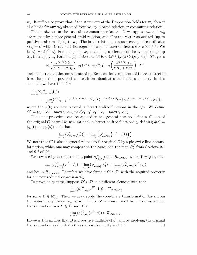
16 KONSTANZE RIETSCH AND LAUREN WILLIAMS

w0. It suffices to prove that if the statement of the Proposition holds for w0 then it

also holds for any w′0 obtained from w0 by a braid relation or commuting relation.

This is obvious in the case of a commuting relation. Now suppose w0 and w′0

are related by a more general braid relation, and C is the vector associated (up to

positive scalar multiple) to w0. The braid relation gives us a change of coordinates

κ(t) = t′ which is rational, homogeneous and subtraction-free, see Section 3.3. We

let t′z := κ(zC · t). For example, if w0 is the longest element of the symmetric group

S3, then applying Formula (1) of Section 3.3 to y1(zc1t1)y2(z

c2t2)y3(zc3t3) ·B

+, gives

y2

(

zc2+c3t2t3zc1t1 + zc3t3

)

y1 (zc1t1 + zc3t3) y2

(

zc1+c2t1t2zc1t1 + zc3t3

)

· B+,

and the entries are the components of t′z. Because the components of t′z are subtraction-

free, the maximal power of z in each one dominates the limit as z → ∞. In this

example, we have therefore

limz→∞

(φ>01,s2s1s2

(t′z))

= limz→∞

(φ>01,s2s1s2

(zc2+c3−max(c1,c3)q1(t), zmax(c1,c3)q2(t), z

c1+c2−max(c1,c3)q3(t)))

where the qi(t) are new rational, subtraction-free functions in the tj ’s. We define

C ′ := (c2 + c3 − max(c1, c3), max(c1, c3), c1 + c2 − max(c1, c3)).

The same procedure can be applied in the general case to define a C ′ out of

the original C as well as new rational, subtraction-free functions qi defining q(t) =

(q1(t), . . . , qr(t)) such that

limz→∞

(φ>0v+,w′

0

(t′z)) = limz→∞

(

φ>0v+,w′

0

(

zC′

· q(t)))

.

We note that C ′ is also in general related to the original C by a piecewise linear trans-

formation, which one may compare to the zones and the map Rj′

j from Sections 9.1

and 9.2 of [26].

We now see by testing out on a point φ>0v+,w′

0

(t′) ∈ Rv,w0;>0, where t′ = q(t), that

limz→∞

(φ>0v+,w′

0

(zC′

· t′)) = limz→∞

(φ>0v+,w′

0

(t′z)) = limz→∞

(φ>0v+,w0

(zC · t)),

and lies in Rv′,w0;>0. Therefore we have found a C ′ ∈ Zr with the required property

for our new reduced expression w′0.

To prove uniqueness, suppose D′ ∈ Zr is a different element such that

limz→∞

(φ>0v+,w′

0(zD′

· t′)) ∈ Rv′,w0;>0

for some t′ ∈ Rr>0. Then we may apply the coordinate transformation back from

the reduced expression w′0 to w0. Thus D′ is transformed by a piecewise-linear

transformation to a D ∈ Zr such that

limz→∞

(φ>0v+,w0

(zD · t)) ∈ Rv′,w0;>0.

However this implies that D is a positive multiple of C, and by applying the original

transformation again, that D′ was a positive multiple of C ′. �

DISCRETE MORSE THEORY FOR TOTALLY NON-NEGATIVE FLAG VARIETIES 17

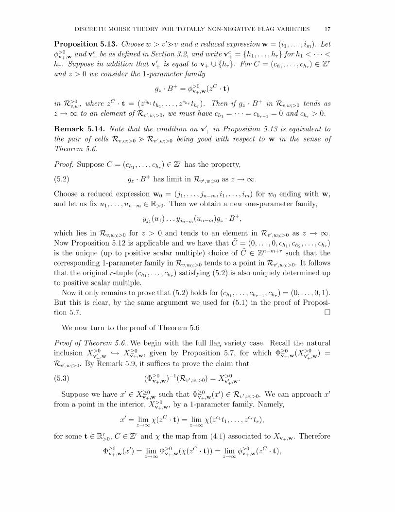
Proposition 5.13. Choose w > v′⋗v and a reduced expression w = (i1, . . . , im). Let

φ>0v+,w and vc

+ be as defined in Section 3.2, and write vc+ = {h1, . . . , hr} for h1 < · · · <

hr. Suppose in addition that v′+ is equal to v+ ∪ {hr}. For C = (ch1

, . . . , chr) ∈ Zr

and z > 0 we consider the 1-parameter family

gz · B+ = φ>0

v+,w(zC · t)

in R>0v,w, where zC · t = (zch1 th1

, . . . , zchr thr). Then if gz · B+ in Rv,w;>0 tends as

z → ∞ to an element of Rv′,w;>0, we must have ch1= · · · = chr−1

= 0 and chr> 0.

Remark 5.14. Note that the condition on v′+ in Proposition 5.13 is equivalent to

the pair of cells Rv,w;>0 ⋗ Rv′,w;>0 being good with respect to w in the sense of

Theorem 5.6.

Proof. Suppose C = (ch1, . . . , chr

) ∈ Zr has the property,

(5.2) gz · B+ has limit in Rv′,w;>0 as z → ∞.

Choose a reduced expression w0 = (j1, . . . , jn−m, i1, . . . , im) for w0 ending with w,

and let us fix u1, . . . , un−m ∈ R>0. Then we obtain a new one-parameter family,

yj1(u1) . . . yjn−m(un−m)gz · B

+,

which lies in Rv,w0;>0 for z > 0 and tends to an element in Rv′,w0;>0 as z → ∞.

Now Proposition 5.12 is applicable and we have that C = (0, . . . , 0, ch1, ch2

, . . . , chr)

is the unique (up to positive scalar multiple) choice of C ∈ Zn−m+r such that the

corresponding 1-parameter family in Rv,w0;>0 tends to a point in Rv′,w0;>0. It follows

that the original r-tuple (ch1, . . . , chr

) satisfying (5.2) is also uniquely determined up

to positive scalar multiple.

Now it only remains to prove that (5.2) holds for (ch1, . . . , chr−1

, chr) = (0, . . . , 0, 1).

But this is clear, by the same argument we used for (5.1) in the proof of Proposi-

tion 5.7. �

We now turn to the proof of Theorem 5.6

Proof of Theorem 5.6. We begin with the full flag variety case. Recall the natural

inclusion X>0v′

+,w

→ X≥0v+,w, given by Proposition 5.7, for which Φ≥0

v+,w(X>0v′

+,w

) =

Rv′,w;>0. By Remark 5.9, it suffices to prove the claim that

(5.3) (Φ≥0v+,w)−1(Rv′,w;>0) = X>0

v′+

,w.

Suppose we have x′ ∈ X≥0v+,w such that Φ≥0

v+,w(x′) ∈ Rv′,w;>0. We can approach x′

from a point in the interior, X>0v+,w, by a 1-parameter family. Namely,

x′ = limz→∞

χ(zC · t) = limz→∞

χ(zc1t1, . . . , zcrtr),

for some t ∈ Rr>0, C ∈ Zr and χ the map from (4.1) associated to Xv+,w. Therefore

Φ≥0v+,w(x′) = lim

z→∞Φ>0

v+,w(χ(zC · t)) = limz→∞

φ>0v+,w(zC · t),

18 KONSTANZE RIETSCH AND LAUREN WILLIAMS

where the 1-parameter subgroup on the right hand side is as in Proposition 5.13.

Since by our assumption Φ≥0v+,w(x′) ∈ Rv′,w;>0, and we are in the ‘good’ situation,

Proposition 5.13 tells us that C = (0, . . . , 0, c), for positive c. But this implies that

x′ = limz→∞

χ(zC · t) ∈ X>0v′

+,w,

see Remark 5.8. Therefore the claim (5.3) holds and the Theorem is true for the full

flag variety.

Now consider the case of G/PJ . We have that πJ gives an isomorphism from

Rxu−1,w;>0 to PJx,u,w;>0 and from Rx′u′−1,w;>0 to PJ

x′,u′,w;>0. We’ve already proved that

Rx′u′−1,w;>0 is a regular face of Rxu−1,w;>0 with respect to the attaching map Φ≥0

xu−1+

,w.

Recall that the attaching map for Px,u,w;>0 is simply πJ ◦ Φ≥0

xu−1+

,w.

When we restrict πJ to Rxu−1,w;>0, it is straightforward to check that the preimage

of PJx′,u′,w;>0 is Rx′u′−1,w;>0. By Theorem 5.6 in the full flag variety case, we know

that (Φ≥0

xu−1+

,w)−1(Rx′u′−1,w;>0) = X>0

x′u′−1+

,wand Φ≥0

xu−1+

,wis a homeomorphism from

X>0x′u′−1

+,w

to Rx′u′−1,w;>0. Therefore (πJ ◦ Φ≥0

xu−1+

,w)−1(Rx′u′−1,w;>0) = X>0

x′u′−1+

,wand

πJ ◦ Φ≥0

xu−1+

,wis a homeomorphism from X>0

x′u′−1+

,wto Rx′u′−1,w;>0. It follows that

PJx′,u′,w;>0 is a regular face of P J

x,u,w;>0 with respect to the attaching map πJ ◦Φ≥0

xu−1+

,w.

�

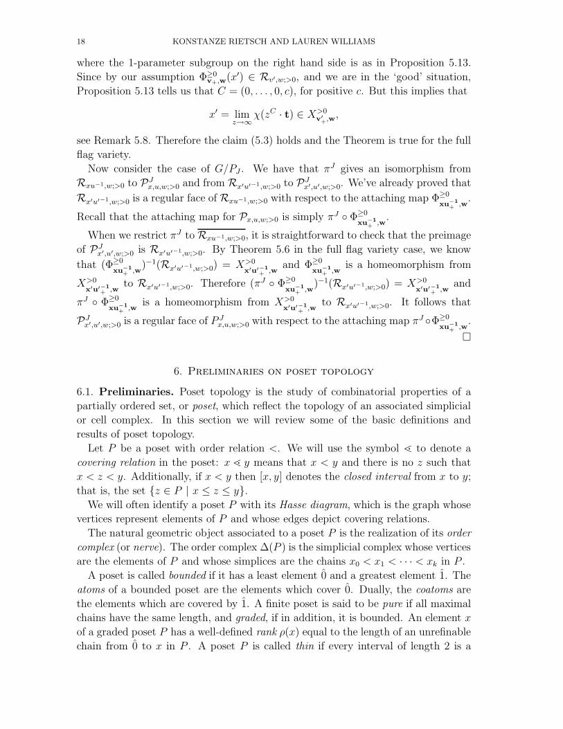
6. Preliminaries on poset topology

6.1. Preliminaries. Poset topology is the study of combinatorial properties of a

partially ordered set, or poset, which reflect the topology of an associated simplicial

or cell complex. In this section we will review some of the basic definitions and

results of poset topology.

Let P be a poset with order relation <. We will use the symbol ⋖ to denote a

covering relation in the poset: x ⋖ y means that x < y and there is no z such that

x < z < y. Additionally, if x < y then [x, y] denotes the closed interval from x to y;

that is, the set {z ∈ P | x ≤ z ≤ y}.

We will often identify a poset P with its Hasse diagram, which is the graph whose

vertices represent elements of P and whose edges depict covering relations.

The natural geometric object associated to a poset P is the realization of its order

complex (or nerve). The order complex ∆(P ) is the simplicial complex whose vertices

are the elements of P and whose simplices are the chains x0 < x1 < · · · < xk in P .

A poset is called bounded if it has a least element 0 and a greatest element 1. The

atoms of a bounded poset are the elements which cover 0. Dually, the coatoms are

the elements which are covered by 1. A finite poset is said to be pure if all maximal

chains have the same length, and graded, if in addition, it is bounded. An element x

of a graded poset P has a well-defined rank ρ(x) equal to the length of an unrefinable

chain from 0 to x in P . A poset P is called thin if every interval of length 2 is a

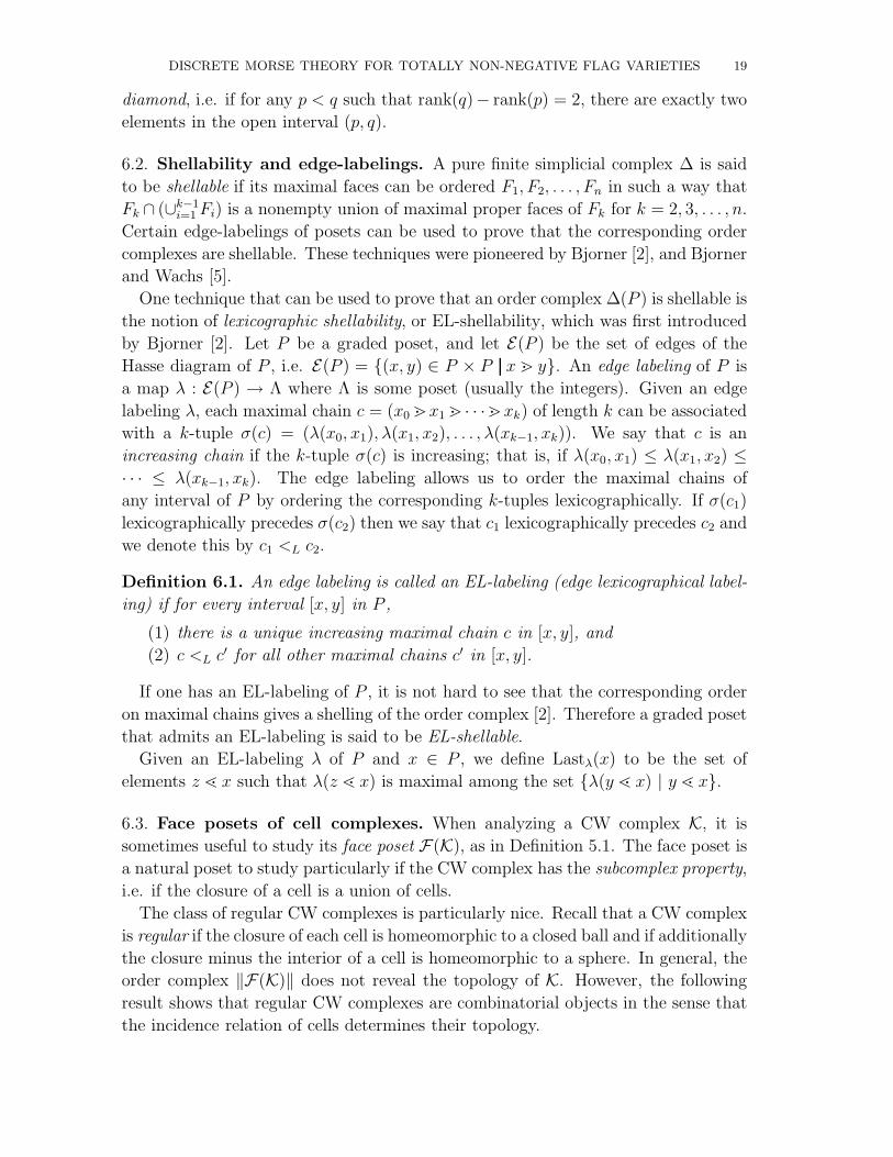
DISCRETE MORSE THEORY FOR TOTALLY NON-NEGATIVE FLAG VARIETIES 19

diamond, i.e. if for any p < q such that rank(q)− rank(p) = 2, there are exactly two

elements in the open interval (p, q).

6.2. Shellability and edge-labelings. A pure finite simplicial complex ∆ is said

to be shellable if its maximal faces can be ordered F1, F2, . . . , Fn in such a way that

Fk ∩ (∪k−1i=1 Fi) is a nonempty union of maximal proper faces of Fk for k = 2, 3, . . . , n.

Certain edge-labelings of posets can be used to prove that the corresponding order

complexes are shellable. These techniques were pioneered by Bjorner [2], and Bjorner

and Wachs [5].

One technique that can be used to prove that an order complex ∆(P ) is shellable is

the notion of lexicographic shellability, or EL-shellability, which was first introduced

by Bjorner [2]. Let P be a graded poset, and let E(P ) be the set of edges of the

Hasse diagram of P , i.e. E(P ) = {(x, y) ∈ P × P x ⋗ y}. An edge labeling of P is

a map λ : E(P ) → Λ where Λ is some poset (usually the integers). Given an edge

labeling λ, each maximal chain c = (x0 ⋗x1 ⋗ · · ·⋗xk) of length k can be associated

with a k-tuple σ(c) = (λ(x0, x1), λ(x1, x2), . . . , λ(xk−1, xk)). We say that c is an

increasing chain if the k-tuple σ(c) is increasing; that is, if λ(x0, x1) ≤ λ(x1, x2) ≤

· · · ≤ λ(xk−1, xk). The edge labeling allows us to order the maximal chains of

any interval of P by ordering the corresponding k-tuples lexicographically. If σ(c1)

lexicographically precedes σ(c2) then we say that c1 lexicographically precedes c2 and

we denote this by c1 <L c2.

Definition 6.1. An edge labeling is called an EL-labeling (edge lexicographical label-

ing) if for every interval [x, y] in P ,

(1) there is a unique increasing maximal chain c in [x, y], and

(2) c <L c′ for all other maximal chains c′ in [x, y].

If one has an EL-labeling of P , it is not hard to see that the corresponding order

on maximal chains gives a shelling of the order complex [2]. Therefore a graded poset

that admits an EL-labeling is said to be EL-shellable.

Given an EL-labeling λ of P and x ∈ P , we define Lastλ(x) to be the set of

elements z ⋖ x such that λ(z ⋖ x) is maximal among the set {λ(y ⋖ x) | y ⋖ x}.

6.3. Face posets of cell complexes. When analyzing a CW complex K, it is

sometimes useful to study its face poset F(K), as in Definition 5.1. The face poset is

a natural poset to study particularly if the CW complex has the subcomplex property,

i.e. if the closure of a cell is a union of cells.

The class of regular CW complexes is particularly nice. Recall that a CW complex

is regular if the closure of each cell is homeomorphic to a closed ball and if additionally

the closure minus the interior of a cell is homeomorphic to a sphere. In general, the

order complex ‖F(K)‖ does not reveal the topology of K. However, the following

result shows that regular CW complexes are combinatorial objects in the sense that

the incidence relation of cells determines their topology.

20 KONSTANZE RIETSCH AND LAUREN WILLIAMS

Proposition 6.2. [4, Proposition 4.7.8] Let K be a regular CW complex. Then K is

homeomorphic to ‖F(K)‖.

We will call a poset P a CW poset if it is the face poset of a regular CW complex.

There is a notion of shelling for regular cell complexes (which is distinct from the

notion of shelling of the order complex), due to Bjorner and Wachs. Such a shelling

is a certain ordering on the coatoms of the face poset. We don’t need the precise

definition, only the following result that an EL-labeling of the augmented face poset

of a regular cell complex gives rise to a shelling.

Theorem 6.3. [7, Theorem 5.11][8, Theorem 13.2] If P is the augmented face poset

of a finite-dimensional regular CW complex K, then any EL-labeling of P gives

rise to a shelling of K. To go from the EL-labeling to the shelling one chooses

the ordering on coatoms which is specified by the order on edges between the unique

greatest element and the coatoms.

7. Discrete Morse theory for general CW complexes

In this section we review Forman’s powerful discrete Morse theory [15]. The the-

ory comes in three “flavors”: for simplicial complexes, regular CW complexes, and

general CW complexes. In each setting, one needs to find a certain discrete Morse

function, and then the main theorem says that the space in question is homotopy

equivalent to another simpler space obtained by collapsing non-critical cells.

The first two flavors of the theory are the simplest and most widely used, because

in these two settings a result of Chari [11] implies that a discrete Morse function

is equivalent to a matching on the face poset of the CW complex. To work with

the third flavor of the theory, one must check some additional technical conditions:

the discrete Morse hypothesis, as well as an extra topological condition included

in the definition of discrete Morse function. However, as we will see in Theorem

7.6, it is enough to find a matching on the face poset of a CW complex with the

subcomplex property such that matched edges are regular. Although this result will

not be surprising to the experts, we could not find it in the literature and so we

give an exposition here. The proof follows from an argument of Kozlov [23, Proof of

Theorem 3.2].1

7.1. Forman’s discrete Morse theorem for general CW complexes. Let K

be a finite CW complex and let Q be its poset of cells. Recall the definition of regular

face from Definition 5.5.

Definition 7.1. [15, p. 102] A function f : Q → R is a discrete Morse function if

for every σ(p) of dimension p, the following conditions hold:

(1) #{τ (p+1)|τ (p+1) > σ and f(τ) ≤ f(σ)} ≤ 1

(2) #{v(p−1)|v(p−1) < σ and f(v) ≥ f(σ)} ≤ 1.

1Although Theorem 3.2 of [23] was in the more restricted setting of regular CW complexes, the

proof still holds in our situtation.

DISCRETE MORSE THEORY FOR TOTALLY NON-NEGATIVE FLAG VARIETIES 21

(3) If σ is an irregular face of τ (p+1) then f(τ) > f(σ).

(4) If v(p−1) is an irregular face of σ then f(v) < f(σ).

Note that a Morse function is a function which is “almost increasing”. Indeed, one

should think of a Morse function as a function which specifies the order in which to

attach the cells of a homotopy-equivalent CW complex [23].

Definition 7.2. We say that a cell σ(p) is critical if

(1) #{τ (p+1) > σ | f(τ) ≤ f(σ)} = 0, and

(2) #{v(p−1) < σ | f(v) ≥ f(σ)} = 0.

Let mp(f) denote the number of critical cells of dimension p.

For each cell σ of a CW complex K, let Carrier(σ) denote the smallest subcomplex

of K containing σ. If K has the subcomplex property (see Section 6.3), then for any

σ, Carrier(σ) is its closure, and hence condition (1) of Definition 7.3 below is satisfied.

Definition 7.3. [15, p. 136] Given a CW complex K and a discrete Morse function

f , we say that (K, f) satisfies the Discrete Morse Hypothesis if:

(1) For every pair of cells σ and τ , if τ ⊂ Carrier(σ) and τ is not a face of σ,

then f(τ) ≤ f(σ).

(2) Whenever there is a τ > σ(p) with f(τ) < f(σ) then there is a τ (p+1) with

τ > σ and f(τ) ≤ f(τ).

The following is Forman’s main theorem for general CW complexes.

Theorem 7.4. [15, Theorem 10.2] Let K be a CW complex satisfying the Discrete

Morse Hypothesis, and f a discrete Morse function. Then K is homotopy equivalent

to a CW complex with mp(f) cells of dimension p.

7.2. Discrete Morse functions as matchings. Chari [11] pointed out that when

the CW complex is regular, one can depict a Morse function f as a certain kind of

matching on the Hasse diagram of the poset of cells. Given such an f , we define a

matching M(f) on the Hasse diagram of Q whose edges correspond to the pairs of

cells in which we get equality in (1) or (2) of Definition 7.1.

Recall that a matching of a graph G = (V, E) is a subset M of edges of G such

that each vertex in V is incident to at most one edge of M . We define a Morse

matching M on a poset Q to be a matching on the Hasse diagram such that if edges

in M are directed from lower to higher-dimension elements and all other edges are

directed from higher to lower-dimension elements, then the resulting directed graph

G(M) is acyclic. We refer to any elements of Q which are not matched by M as

critical elements (or critical cells).

In the situation of arbitrary CW complexes, a Morse matching such that matched

edges are regular gives rise to a discrete Morse function satisfying property (2) of the

Discrete Morse Hypothesis, as the following lemma shows. The proof of this lemma

follows an argument of Kozlov [23, Proof of Theorem 3.2].

22 KONSTANZE RIETSCH AND LAUREN WILLIAMS

Lemma 7.5. Let M be a Morse matching on the face poset Q of a CW complex, such

that each edge in M corresponds to a regular pair of faces in the CW complex. Then

there exists a discrete Morse function fM , satisfying property (2) of the Discrete

Morse Hypothesis, whose critical cells are exactly the critical cells of M .

Proof. We will inductively assign positive integer labels to each of the elements of

Q, producing a function fM . Moreover, fM will have the property that if x < y,

fM (x) ≤ fM(y), with fM(x) = fM(y) if and only if (x, y) ∈ M ; in the case that

(x, y) ∈ M , we will label x and y at the same time.

At each step, let x be one of the elements of Q of minimal rank (dimension) among

those not yet labeled, and let i be the smallest positive integer not yet appearing as

a label in Q. If x is not in M and hence critical, label x with i. If x is not critical,

then we must have (x, y) ∈ M , where x ⋖ y. If each z < y in Q is labeled, then label

both x and y with i. Otherwise, there exists x1 < y in Q where x1 is not labeled;

repeat the argument with x1 taking the place of x. Either we will label x1 or a pair

(x1, y1) ∈ M , or, since G(M) is acyclic, we will find x2 6= x, x2 6= x1, y1 > x2, etc.

Since there are finitely many elements of Q, the process will terminate. Since we

never label an element y ∈ Q until we have labeled each x < y, fM has the property

that for x < y, fM(x) ≤ fM(y). Therefore condition (2) of the Discrete Morse

Hypothesis is satisfied. The only case in which fM(x) = fM(y) is when (x, y) ∈ M ,

i.e. (x ⋖ y) is a regular pair of faces – and so conditions (3) and (4) of Definition 7.1

are satisfied. Conditions (1) and (2) of Definition 7.1 are satisfied because M is a

matching. Finally, it is clear that the cells which are critical with respect to M are

exactly those which are critical with respect to Definition 7.2. �

We now restate Forman’s Morse Theorem for general CW complexes in terms of

Morse matchings.

Theorem 7.6. Let K be a CW complex with the subcomplex property. Suppose its

face poset Q has a Morse matching M , such that whenever (σ(p), τ (p+1)) ∈ M , σ is

a regular face of τ . Let mp(M) denote the number of critical cells of dimension p.

Then K is homotopy equivalent to a CW complex with mp(M) cells of dimension p.

Proof. By Lemma 7.5, we have a discrete Morse function f for K satisfying condi-

tion (2) of Definition 7.3. Since K has the subcomplex property, condition (1) of

Definition 7.3 is satisfied. The result now follows from Theorem 7.4. �

7.3. From edge-labelings to Morse matchings. Both lexicographic shellability

and discrete Morse theory are combinatorial tools which can be used to investigate

the topology of a CW complex. In this section we will recall a result of Chari [11],

which proves the existence of a certain Morse matching given a shelling of a regular

CW complex. We will translate this into a statement about constructing a Morse

matching from an EL -labeling, and note that one can gain some fairly explicit

information about the Morse matching from the EL-labeling.

DISCRETE MORSE THEORY FOR TOTALLY NON-NEGATIVE FLAG VARIETIES 23

Recall the notion of pseudomanifold, e.g. from [11]. Note that by a result of Bing

[4, Chapter 4], a shellable pseudomanifold is in particular a regular CW complex

which is either a ball or a sphere.

Proposition 7.7. [11, Proposition 4.1] Let σ1, σ2, . . . , σm be a shelling of a d-

pseudomanifold Σ and let v be any vertex in σ1. Then the face poset of Σ admits a

Morse matching M such that:

• If Σ is the d-sphere then v and σm are the only critical cells, while if Σ is a

d-ball, then v is the only critical cell.

By Theorem 6.3, an EL-labeling of the augmented face poset of a pseudomanifold

gives rise to a shelling. Chari used induction to construct the Morse matching of

Proposition 7.7. Chari’s proof of Proposition 7.7, applied to a shelling which comes

from an EL-labeling, implies the following.

Corollary 7.8. Suppose that λ is an EL-labeling of the augmented face poset Q of a

pseudomanifold Σ. Let Mλ be the Morse matching given by Proposition 7.7. Every

(σ ⋖ τ) ∈ M has the following property: σ ∈ Lastλ(τ).

In fact, when the edge labels in λ come from a totally ordered set, Chari’s proof

of Proposition 7.7 gives the following algorithm for obtaining the Morse matching.

Corollary 7.9. Suppose that λ is an EL-labeling of the augmented face poset Q of

a pseudomanifold Σ. Then the Morse matching Mλ given by Proposition 7.7 can be

constructed as follows. Set n equal to the rank of the poset Q and set M = ∅.

(1) Consider all unmatched elements σ of rank n, and for each, add Lastλ(σ)⋖σ

to M .

(2) Decrease n by 1 and go to step 1.

Remark 7.10. Chari also extends Proposition 7.7 to regular CW complexes [11,

Theorem 4.2]. Corollaries 7.8 and 7.9 also hold in this situation.

Remark 7.11. Proposition 7.7 and Corollary 7.8 can be useful even when K is a

CW complex not known to be regular. In particular, if the face poset Q of K is a CW

poset, then there exists a regular CW complex Kreg whose face poset is Q. Therefore

one can still use these results to construct a Morse matching of K.

8. The Bruhat order, shellability, and reduced expressions

Fix a Coxeter system (W, I) and let T be the set of reflections. In this section we

will review some properties of the Bruhat order ≤ and prove a result (Proposition

8.8) about reduced expressions which will be needed for the proof of Proposition 9.5.

The first part of Theorem 8.1 below is due to Bjorner and Wachs [5]. The second

part follows from the first together with Bjorner’s result [3] characterizing CW posets.

24 KONSTANZE RIETSCH AND LAUREN WILLIAMS

Theorem 8.1. [5] [3] The Bruhat order of a Coxeter group is thin and (CL)-shellable.

Furthermore, an interval with at least two elements is the augmented face poset of a

regular CW complex homeomorphic to a ball. 2

Theorem 8.1 together with Proposition 7.7 imply the following.

Corollary 8.2. Let v < w in the Bruhat order of a Coxeter group. Then if we remove

v from the interval [v, w] (which plays the role of 0), there is a Morse matching M

on the resulting poset with one critical element u of minimal rank. Adding v back to

the poset and adding the edge (v, u) to M , we get a Morse matching on [v, w] with

no critical elements.

Dyer [14] subsequently strengthened the Bjorner-Wachs result by giving an EL-

labeling of Bruhat order. Dyer’s primary tool was his notion of “reflection orders,”

certain total orderings of T which can be characterized as follows.

Definition 8.3. [14, Proposition 2.13] Let (W, I) be a finite Coxeter system with

longest element w0, and let T = {t1, . . . , tn} (n = ℓ(w0)). Then the total order

t1 ≺ t2 ≺ · · · ≺ tn on T is a reflection order if and only if there is a reduced

expression w0 = si1 . . . sin such that tj = si1 . . . sij−1sijsij−1

. . . si1, for 1 ≤ j ≤ n.

Remark 8.4. [14, Remark 2.4] The reverse of a reflection order is a reflection order.

Proposition 8.5. [14] Fix a reflection order � on T . Label each edge x ⋗ y of the

Bruhat order by the reflection x−1y. Then this edge labeling together with � is an

EL-labeling; therefore the Bruhat order is EL-shellable.

In what follows, the notation sk indicates the omission of the factor sk.

Definition 8.6. [19] Consider a Coxeter system (W, I). Define a deletion pair in

an expression si1 . . . sid to be a pair sir , sit (where r < t) such that the subexpression

sir . . . sit is not reduced but sir . . . sit and sir . . . sit are each reduced.

E.g. in type A the first s1 and the last s2 in s1s2s1s2 comprise a deletion pair.

Lemma 8.7. [19, Lemma 3.31] If sir . . . siu . . . sit is reduced but sir . . . sit is not, then

siu belongs to a deletion pair within sir . . . sit.

Proposition 8.8. Consider x ≤ w in a Coxeter group W , and fix a reduced ex-

pression w = (i1, . . . , it) for w. Let x+ = {j1, . . . , jk}. For any p ≤ t, consider the

product γ1 . . . γt, where

γr =

{

sir , if r ∈ x+ or r ≥ p,

1 otherwise.

Then γ1 . . . γt is reduced.

2Recall from Remark 5.2 that [5] augments the poset of cells with a 0 and also a greatest element

1. Using this convention, [5] considers intervals in Bruhat order to be posets associated to regular

CW complexes homeomorphic to spheres.

DISCRETE MORSE THEORY FOR TOTALLY NON-NEGATIVE FLAG VARIETIES 25

Proof. We will prove this by induction. First consider p = t. If it ∈ x+ there is

nothing to prove, since sij1. . . sijk

is reduced. If it /∈ x+ then assume that γ1 . . . γt

is not reduced. This means that xsit < x, which contradicts the fact that x+ is the

positive subexpression for x.

Now by induction assume the proposition holds for any p between some p′ and t,

where p′ ≤ t. We want to prove it for p := p′ − 1. First suppose that p′ − 1 ∈ x+.

In this case the product γ1 . . . γt is the same for both p = p′ and p = p′ − 1: in both

cases, γp′−1 = sip′−1. Therefore by induction it follows that γ1 . . . γt is reduced.

Now suppose that p′ − 1 /∈ x+. In this case the induction hypothesis tells us only

that γ1 . . . γp′−2γp′ . . . γt is reduced; we need to prove that γ1 . . . γp′−2γp′−1γp′ . . . γt =

γ1 . . . γp′−2sip′−1sip′

. . . sit is reduced. Assume it is not: then by Lemma 8.7, sip′−1

belongs to a deletion pair within γ1 . . . γp′−2sip′−1sip′

. . . sit . Note that sip′−1sip′

. . . sit

comprises a consecutive string of generators in a reduced expression and so must

be reduced. Also note that by our argument in the first paragraph, γ1 . . . γp′−2sip′−1

must be reduced: otherwise γ1 . . . γp′−2sip′−1< γ1 . . . γp′−2, which contradicts the

fact that x+ is a positive subexpression and does not contain sip′−1. But we’ve now

shown that sip′−1cannot belong to a deletion pair within γ1 . . . γp′−2sip′−1

sip′. . . sit , a

contradiction. �

9. Morse matchings and the proof of contractibility

In this section we will construct a Morse matching on the face poset of the closure

of an arbitrary cell of (G/P )≥0, such that matched edges are provably regular. We

will then use this to prove our main result: that the closure of each cell is contractible,

and the boundary of each cell is homotopy equivalent to a sphere.

Recall the definition of the augmented face poset QJ of (G/PJ)≥0 from Section

5. Besides having a unique least element 0, QJ also has a unique greatest element:

This is 1 := PJu0,u0,w0;>0, where u0 and wJ

0 are the longest elements in WJ and W J ,

respectively.

The following was proved in [40].

Theorem 9.1. [40] QJ is graded, thin, and EL-shellable. It follows that the face

poset of (G/PJ)≥0 is the face poset of a regular CW complex homeomorphic to a ball.

It will be useful for us to classify the cover relations in QJ . The following classifi-

cation is analogous to the one used in [40], with the roles of x and w reversed.

Lemma 9.2. The cover relations in QJ fall into the following three categories.

Type 1: PJx′,v,w;>0 ⋖ PJ

x,u,w;>0 such that x < x′. It follows that xu−1 ⋖ x′v−1.

Type 2: PJx,v,w′;>0 ⋖ PJ

x,u,w;>0 such that w′ ≤ w. It follows that w′v ⋖ wu.

Type 3: 0 ⋖ PJx,u,w;>0 where PJ

x,u,w;>0 is a 0-cell. It follows that x = wu.

Remark 9.3. If Q is a poset, then the interval poset Int(Q) is defined to be the

poset of intervals [x, y] of Q, ordered by containment. When G/PJ is the complete

flag variety, i.e. when J = ∅, QJ is simply the interval poset of the Bruhat order.

26 KONSTANZE RIETSCH AND LAUREN WILLIAMS

Theorem 9.4. Choose any cell PJx,u,w;>0 of (G/PJ)≥0. Then there is a Morse match-

ing on the face poset of PJx,u,w;>0 with a single critical cell of dimension 0, which re-

stricts to a Morse matching on the face poset of the boundary bd(PJx,u,w;>0) with one

additional critical cell of top dimension. Furthermore, all matched edges are good:

that is, if PJx′,u′,w′;>0 ⋖ PJ

x,u,w;>0 are matched, then w′ = w and there is a reduced

expression (i1, . . . , im) of w such that the positive subexpression x′u′−1

+ is equal to

xu−1

+ ∪ {k} and moreover xu−1

+ contains {k + 1, . . . , m}.

We will prove Theorem 9.4 in a series of steps. Define Sx(w) := {Rv,w;>0|x ≤ v ≤

w}, and give this the poset structure inherited from QJ (for J = ∅). This poset is

isomorphic to the (dual of the) Bruhat interval between x and w.

Proposition 9.5. Sx(w) has a Morse matching Mx(w) in which all matched edges

are good. If x < w, then Mx(w) has no critical cells. If x = w, Mx(w) has one

critical cell.

Proof. We will construct Mx(w) by using Dyer’s EL-labeling of the Bruhat interval

(Proposition 8.5) and Chari’s observation that one can go from a shelling to a Morse

matching (Proposition 7.7). To deduce that matched edges are good, we will choose

our reflection order carefully and use Corollary 7.8.

Fix a reduced expression w = (i1, . . . , im) for w, and choose a reduced expression

for w0 which begins with w−1. By Definition 8.3, this gives a reflection order. Let

≺ be the reverse of this order; by Remark 8.4, ≺ is also a reflection order.

Label the edge Rv′,w;>0 ⋖ Rv,w;>0 (where v′ ⋗ v) in Sx(w) with the reflection τ

such that v = v′τ . By Proposition 8.5, this gives an EL-labeling of Sx(w). If Sx(w)

has at least two elements then by Corollary 8.2, there is a Morse matching Mx(w)

on Sx(w) with no critical cells. Otherwise, if Sx(w) has one element, i.e. if x = w,

then we take Mx(w) to be the empty matching with one critical cell.

We now need to show that all edges in Mx(w) are good. By Corollary 7.8, if τ

labels the edge Rv,w;>0 ⋗Rv′,w;>0 (for v′ ⋗ v) and this edge is in Mx(w), then among

all edge labels going from Rv,w;>0 to lower-dimensional cells, τ is maximal in ≺. So

we need to analyze cover relations corresponding to maximal labels.

Let v+ = {j1, . . . , jr}. Let k be maximal (1 ≤ k ≤ m) such that k /∈ {j1, . . . , jr}.

We first claim that u = {j1, . . . , jr} ∪ {k} is a reduced subexpression of w, hence

Ru,w;>0 ⋖ Rv,w;>0, and that u is positive. Second, we claim that the label on the

edge from Rv,w;>0 to Ru,w;>0 is maximal among all edge labels from Rv,w;>0 down to

a lower-dimensional cell.

Proposition 8.8 implies the first claim that {j1, . . . , jr} ∪ {k} is a reduced subex-

pression of w. Knowing that it is reduced, it is clear that it is positive.

To see that the second claim is true, note that by the choice of k, the label on

the edge Rv,w;>0 ⋗Ru,w;>0 is u−1v = simsim−1. . . sik . . . sim−1

sim . Furthermore, in our

reflection order, sim ≻ simsim−1sim ≻ · · · ≻ simsim−1

. . . sik . . . sim−1sim ≻ . . . . Since k

is maximal such that k /∈ {j1, . . . , jr}, if we define v′′

= vsimsim−1. . . siℓ . . . sim−1

sim

for ℓ > k, then ℓ ∈ {j1, . . . , jr} so an expression for v′′

is given by {j1, . . . , jr} \

DISCRETE MORSE THEORY FOR TOTALLY NON-NEGATIVE FLAG VARIETIES 27

{ℓ}. In particular, v′′

< v and so Rv,w;>0 does not cover Rv′′

,w;>0. On the other

hand, we know that Rv,w;>0 covers Ru,w;>0, and that the label on this edge is

simsim−1. . . sik . . . sim−1

sim . By our choice of reflection order, this label is maximal

among all edges from Rv,w down to lower-dimensional cells.

Finally, by the choice of k, and since {j1, . . . , jr} ∪ {k} = u is positive, this cover

relation is good. Therefore every matched edge in Mx(w) is good. �

Remark 9.6. Recently Brant Jones has constructed explicit matchings of the Hasse

diagram of an interval in Bruhat order; he also proved that his matchings coincide

with the matchings Mx(w) that we constructed in Proposition 9.5 [21].

Remark 9.7. If x is the identity element in W , then the Morse matching constructed

in Proposition 9.5 will actually be a multiplication matching by a Coxeter generator.

This is a so-called special matching, and is relevant to Kazhdan-Lusztig theory [10].

Anders Bjorner suggested using special matchings to construct acyclic matchings,

and realized that one could use them to obtain an acyclic matching for the face poset

of the entire space (G/B)≥0 [9]. We are grateful for his insights.

We now turn to the proof of Theorem 9.4

Proof. We partition the elements of the face poset of the closure of PJx,u,w;>0 into

subsets SJxu−1(y) = {PJ

x′,u′,y;>0 | xu−1 ≤ x′u′−1 ≤ y}, for each y ∈ W J such that

xu−1 ≤ y ≤ w. By Lemma 9.2, the restriction of the face poset QJ to SJxu−1(y) is

isomorphic to the (dual of the) Bruhat interval between xu−1 and y, so SJxu−1(y) and

Sxu−1(y) are isomorphic as posets: we simply identify PJa,b,y;>0 with Rab−1,y;>0.

We can now apply Proposition 9.5, which gives us a Morse matching MJxu−1(y) on

SJxu−1(y) such that all matched edges are good. This matching has either zero or one

critical cell, based on whether xu−1 < y or xu−1 = y.

We now define

MJx,u,w = ∪y∈W J ,xu−1≤y≤wMJ

xu−1(y).

Since each MJxu−1(y) is a matching, and any two matched elements PJ

a,b,y;>0 and

PJa′,b′,y;>0 in MJ

x,u,w have the same third factor y, MJx,u,w is also a matching.

Let us assume for the sake of contradiction that there is a cycle in G(MJx,u,w).

Since each G(MJxu−1(y)) is acyclic, there must be some edges in the cycle which pass

between two different SJxu−1(y)’s. Each such edge must be directed from the higher-

dimensional cell PJa,b,y;>0 to the lower-dimensional cell PJ

a′,b′,y′;>0 for y 6= y′, so by

Lemma 9.2, y′ < y. So if we traverse the cycle and look at the sequence of poset

elements PJ∗,∗,y;>0 that we encounter, the third factor can only decrease. Therefore

it is impossible to return to the element of the cycle at which we started, which is a

contradiction.

As y varies over elements of W J between xu−1 and w, we have that MJxu−1(y) has

no critical cells for xu−1 < y and it has one critical cell PJx,u,xu−1;>0 for xu−1 = y.

Therefore MJx,u,w has a unique critical cell, the 0-dimensional cell PJ

x,u,xu−1;>0.

28 KONSTANZE RIETSCH AND LAUREN WILLIAMS

Since the face poset of PJx,u,w;>0 has a unique cell of top dimension ℓ(w)− ℓ(xu−1)

which is matched in MJx,u,w, when we restrict MJ

x,u,w to the boundary bd(PJx,u,w;>0),

we will get a Morse matching with one additional critical cell of top dimension

ℓ(w) − ℓ(xu−1) − 1. This completes the proof of the theorem. �

Corollary 9.8. Choose any cell PJx,u,w;>0 of (G/PJ)≥0. Then there is a Morse match-

ing on the face poset of PJx,u,w;>0 with a single critical cell of dimension 0 in which

all matched edges are regular; it restricts to a Morse matching on the face poset of

the boundary bd(PJx,u,w;>0) with one additional critical cell of top dimension.

Proof. This follows from Theorem 5.6 and Theorem 9.4. �

We now prove our main result.

Theorem 9.9. The closure of each cell of (G/P )≥0 is contractible, and the boundary

of each cell of (G/P )≥0 is homotopy equivalent to a sphere.

Proof. Choose an arbitrary cell of (G/P )≥0 and let K be its closure. Note that K is

a CW complex with the subcomplex property because Theorems 4.5 and 5.3 imply

that (G/P )≥0 is. Let Q be the face poset of K. By Corollary 9.8, Q has a Morse

matching with a unique critical cell of dimension 0, in which all matched edges are

regular. Therefore Theorem 7.6 implies K is contractible.

Now let K ′ be the boundary of an arbitrary cell and let Q′ be its face poset. By

Corollary 9.8, Q′ has a Morse matching with two critical cells, one of dimension 0

and one of top dimension, say p, in which all matched edges are regular. Therefore

Theorem 7.6 implies that K ′ is homotopy equivalent to a CW complex with one

0-dimensional cell σ and one p-dimensional cell whose boundary is glued to σ. This

is precisely a p-sphere. �

Remark 9.10. Since a Morse function actually gives rise to a concrete collapsing

[15] of a CW complex, in fact we have shown that the closure of a cell is collapsible.

Remark 9.11. One can give a simpler proof that the closure of each cell in the totally

non-negative part of the type A Grassmannian (Grkn)≥0 is contractible. In that case,

one can prove directly that whenever a cell σ has codimension 1 in the closure of τ ,

then σ is a regular face of τ . This follows from the technology of [31]: in particular,

Theorem 18.3, Lemma 18.9, and Corollary 18.10. Then by Theorem 9.1, the poset

of cells of (Grkn)≥0 is a CW poset with an EL-labeling (hence a shelling), so by

Proposition 7.7, we have the requisite Morse matching.

Using Corollary 7.9, we see that there is a more concrete way to describe the

matchings Mx(w) of Sx(w).

Remark 9.12. Fix a reduced expression w = (i1, . . . , im) for w. Start with the

maximal element Rx,w;>0. Let k be maximal such that 1 ≤ k ≤ m and k /∈ x+. Then

x+ ∪ {k} is the positive subexpression for an element v > x. We match Rx,w;>0 to

Rv,w;>0. Now apply the same procedure to every element of dimension dimRx,w;>0−1

DISCRETE MORSE THEORY FOR TOTALLY NON-NEGATIVE FLAG VARIETIES 29

which has not been matched (the order in which we consider these elements does not

matter). Continue in this fashion, from higher to lower-dimensional cells.

References

[1] A. Berenstein, A. Zelevinsky, Tensor product multiplicities, canonical bases and totally positive

varieties, Invent. math., 143 (2001), no. 1, 77–128.

[2] A. Bjorner, Shellable and Cohen-Macaulay partially ordered sets, Trans. Amer. Math. Soc. 260

(1980), 159–183.

[3] A. Bjorner, Posets, regular CW complexes and Bruhat order, Europ. J. Combin. 5 (1984), 7–16.

[4] A. Bjorner, M. Law Vergnas, B. Sturmfels, N. White, G. Ziegler, Oriented Matroids, Cambridge

University Press, 1993.

[5] A. Bjorner, M. Wachs, Bruhat order of Coxeter groups and shellability, Adv. Math. 43 (1982)

87–100.

[6] A. Bjorner, M. Wachs, On lexicographically shellable posets, Trans. Amer. Math. Soc. 277

(1983), 323–341.

[7] A. Bjorner, M. Wachs, Shellable nonpure complexes and posets I, Trans. Amer. Math. Soc. 348

(1996), no. 4, 1299–1327.

[8] A. Bjorner, M. Wachs, Shellable nonpure complexes and posets II, Trans. Amer. Math. Soc.

349 (1997), no. 10, 3945–3975.

[9] A. Bjorner, personal communication to L. Williams, Mittag-Leffler Institute, May 2005.

[10] F. Brenti, F. Caselli, M. Marietti, Special matchings and Kazhdan-Lusztig polynomials, Adv.

Math. 202 (2006), 555–601.

[11] M. Chari, On discrete Morse functions and combinatorial decompositions, Discrete Math 217

(2000), 101 – 113.

[12] G. Danaraj, V. Klee, Shellings of spheres and polytopes, Duke Math. J. 41 (1974), 443–451.

[13] V. Deodhar, A combinatorial setting for questions in Kazhdan-Lusztig theory, Geometriae

Dedicata 36 (1990), 95–119.

[14] M. Dyer, Compos. Math. 89 (1993), 91–115.

[15] R. Forman, Morse theory for cell complexes, Adv. Math. 134 (1998), no. 1, 90–145.

[16] R. Forman, A user’s guide to discrete Morse theory, Sem. Lothar. Combin. 48 (2002), Art.

B48c, 35pp. (electronic).

[17] W. Fulton, Introduction to toric varieties, Annals of Mathematics Studies, 131. The William

H. Roever Lectures in Geometry, Princeton University Press, Princeton, NJ, 1993.

[18] K. R. Goodearl, M. Yakimov, Poisson structures on affine spaces and flag varieties II. General

case, arXiv:math.QA/0509075 (to appear in Trans. AMS)

[19] P. Hersh, Regular cell complexes in total positivity, arXiv:0711.1348.

[20] J. Humphreys, Reflection groups and Coxeter groups, Cambridge University Press, 1990.

[21] B. Jones, An explicit derivation of the Mobius function for Bruhat order, arXiv:0904.4472.

[22] D. Kazhdan, G. Lusztig, Representations of Coxeter groups and Hecke algebras, Invent. Math.,

53 (1979), 165–184.

[23] D. Kozlov, Collapsibility of ∆(Πn)Sn and some related CW complexes, Proc. Amer. Math.

Soc. 128 (2000), no. 8, 2253–2259.

[24] G. Lusztig, Canonical bases arising from quantized enveloping algebras, J. Amer. Math. Soc.

3 (1990), 447–498.

[25] G. Lusztig, Introduction to Quantum Groups, Progr. in Math. 110, Birkhauser Boston, 1993,

341 pages.

[26] G. Lusztig, Total positivity in reductive groups, in: Lie theory and geometry: in honor of

Bertram Kostant, Progress in Mathematics 123, Birkhauser, 1994.

30 KONSTANZE RIETSCH AND LAUREN WILLIAMS

[27] G. Lusztig, Introduction to total positivity, in Positivity in Lie theory: open problems, ed. J.

Hilgert, J.D. Lawson, K.H. Neeb, E.B. Vinberg, de Gruyter Berlin, 1998, 133–145.

[28] G. Lusztig, Total positivity in partial flag manifolds, Representation Theory, 2 (1998) 70–78.

[29] G. Lusztig, personal communication with K. Rietsch, Oberwolfach, 1996.

[30] R. Marsh, K. Rietsch, Parametrizations of flag varieties, Representation Theory, 8 (2004).

[31] A. Postnikov, Total positivity, Grassmannians, and networks, arXiv:math.CO/0609764.

[32] A. Postnikov, D. Speyer, L. Williams, Matching polytopes, toric geometry, and the non-

negative part of the Grassmannian, to appear in J. Alg. Combin.

[33] K. Rietsch, Total positivity and real flag varieties, Ph.D. Dissertation, MIT, 1998.

[34] K. Rietsch, Closure relations for totally non-negative cells in G/P , Math. Res. Let. 13 (2006),

775–786.

[35] K. Rietsch, A mirror symmetric construction for qH∗T(G/P ), Adv. Math. 217 (2008), 2401–

2442.

[36] K. Rietsch, L. Williams, The totally non-negative part of G/P is a CW complex, Transforma-

tion Groups 13, Special volume in honor of B. Kostant’s 80th birthday, (2008), 839–953.

[37] F. Sottile, Toric ideals, real toric varieties, and the moment map. Topics in algebraic geometry

and geometric modeling, 225–240, Contemp. Math., 334, Amer. Math. Soc., Providence, RI,

2003.

[38] R. Steinberg, Endomorphisms of linear algebraic groups, Memoirs of the Amer. Math. Soc.,

80, Amer. Math. Soc., Providence, RI, 1968.

[39] M. Wachs, Poset topology: tools and applications. Geometric combinatorics, 497–615, IAS/

Park City Math. Ser., 13, Amer. Math. Soc., Providence, RI, 2007.

[40] L. Williams, Shelling totally non-negative flag varieties, J. Reine Angew. Math. 609, 2007.

Department of Mathematics, King’s College London, Strand, London WC2R 2LS

Department of Mathematics, Harvard University, Cambridge, MA 02138

E-mail address : konstanze.rietsch@kcl.ac.uk

E-mail address : lauren@math.harvard.edu