Embed Size (px)
Citation preview
Discrete Mathematics
MA 2201 / CS 2022
Pi Fisher
A Term 2015
1 Course Description
Welcome to Discrete Mathematics. Office hours are Tuesday and Thursday 1100– 1200. The website for the course is at http://web.cs.wpi.edu/~gsarkozy.Conferences are on Wednesdays, and they are the best place to ask questions ifyou are confused about the lectures or homeworks.
The topics we will cover include functions and relations, sets, counting, graphs,algorithms, and logic. This course is a collection of many different parts ofmathematics and computer science. Expect that different sections will be easieror harder for different students.
Weekly homework assignments will be given (usually) on Mondays and returnedthe following Mondays. The two lowest grades for these will be dropped, andthe rest will count for 1/3 of your grade. Working in groups is encouraged, butyou must write your final copy individually. The rest of your grade will be amidterm on September 22 and a final exam on October 15. These will each be1/3 of your grade. The final exam will be cumulative, but will mostly cover thesecond half of the year.
2 Propositional Logic
A proposition is a statement that is either true or false. Statements can’t bein between. We denote these as T and F. The statement that 1 + 1 = 2 is a Tproposition. The statement that 2 + 2 = 5 is a F proposition. The statement
1
MA 2201 / CS 2022 Discrete Mathematics
that X+1 = 3 is not a proposition, because it is sometimes true and sometimesfalse.
2.1 Logical Operators
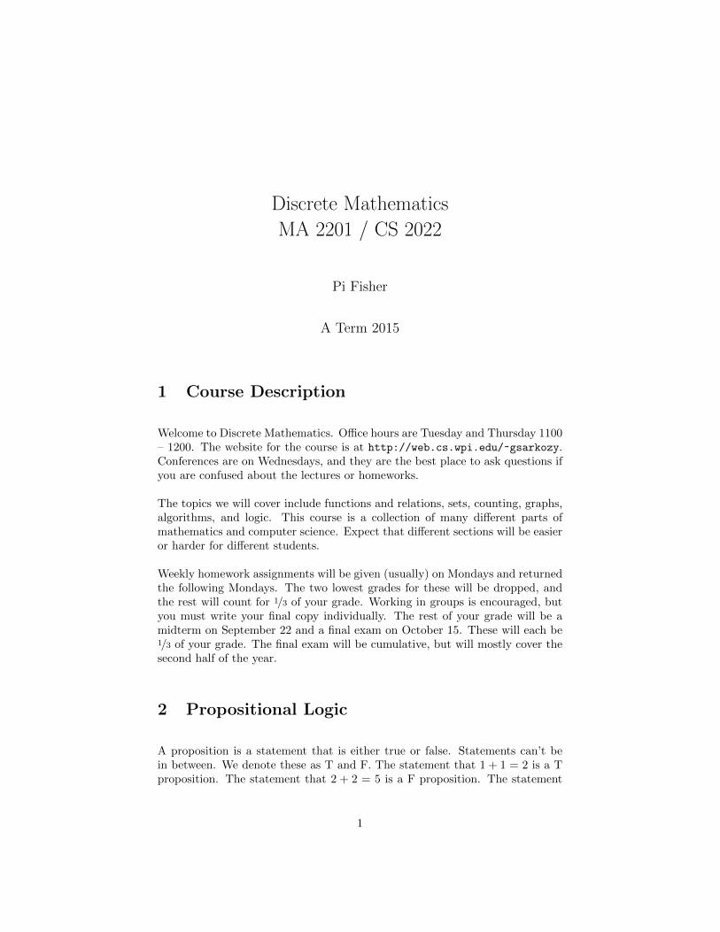
Using logical operators, we can build compound propositions. Our first operatoris negation. If we have a proposition p, we denote the negation as ¬p. Forexample, if p is the proposition “Today is Thursday,” then ¬p would be “Todayis not Thursday.” We use truth tables to see how logical operators work.
p ¬pT FF T
Next we have conjunction (AND), which relies on two propositions, p and q.We denote it as p ∧ q. It is T when both p and q are T. For example, “Todayis Thursday AND we have CS 2022 today.” The truth table is:
p q p ∧ qT T TT F FF T FF F F
If we have two propositions, our truth table will have 2× 2 = 4 possibilities inour table. If we have three, we would have eight possibilities. Be certain to notforget some of them when writing the tables.
Our third operator is disjunction (OR), which also relies on two propositions.p ∨ q is T when any of p and q are T. An example is “Today is Thursday ORwe have CS 2022 today.” This is an “inclusive” OR, meaning that it is T evenif both are T. The truth table is:
p q p ∨ qT T TT F TF T TF F F
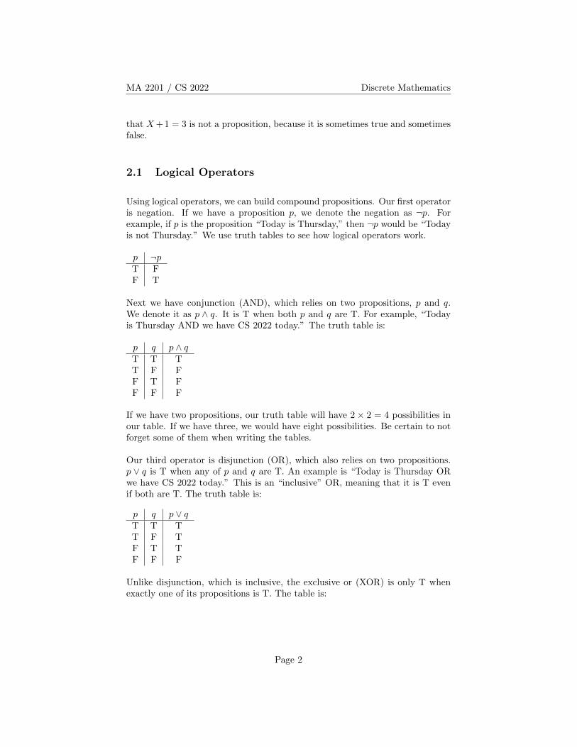
Unlike disjunction, which is inclusive, the exclusive or (XOR) is only T whenexactly one of its propositions is T. The table is:
Page 2
MA 2201 / CS 2022 Discrete Mathematics
p q p⊕ qT T FT F TF T TF F F
Next is implication. This is tricky because it is different from how we use it inEnglish. The notation is p→ q, and it is read as either “if p then q”, “p impliesq”, “p is sufficient for q”, and “p only if q”. That last one is a bit more tricky.Let’s look at the truth table:
p q p→ qT T TT F FF T TF F T
The thing that seems strange is that, when p is F, the implication is T. The lastway of wording the implication means that, if both p and p → q are T, q hasto be T. An example of a typical implication would be, “If today is Thursday,then we have CS 2022 today.” However, in Discrete Mathematics, the followingstatement is also a T statement: “If 2 + 2 = 5, then 2 + 2 = 4.” If the premiseis false, it doesn’t matter what comes later, as anything can follow from a falsepremise. We could even say “If 2 + 2 = 5, then monkeys are purple,” and itwould be T. Unlike in English, the propositions in implications don’t need tobe related.
2.2 Related Propositions
If we have a proposition p → q, then we define its converse as q → p. Wealso define the contrapositive as ¬q → ¬p. If our original implication is “Iftoday is Thursday, then we have CS 2022 today,” then the converse is “If wehave CS 2022 today, then today is Thursday.” Note that this statement is T onThursdays. The contrapositive is “If we don’t have CS 2022 today, then today isnot Thursday.” Note that the contrapositive and original statement are alwaysequivalent. If either is T, so is the other.
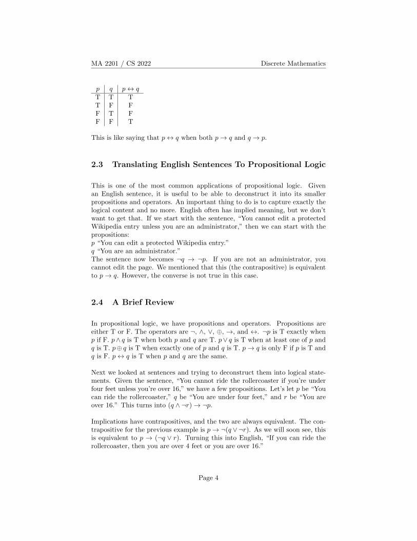
Lastly, we have the Biconditional operator. p↔ q is T only when p and q havethe same value.
Page 3
MA 2201 / CS 2022 Discrete Mathematics
p q p↔ qT T TT F FF T FF F T
This is like saying that p↔ q when both p→ q and q → p.
2.3 Translating English Sentences To Propositional Logic
This is one of the most common applications of propositional logic. Givenan English sentence, it is useful to be able to deconstruct it into its smallerpropositions and operators. An important thing to do is to capture exactly thelogical content and no more. English often has implied meaning, but we don’twant to get that. If we start with the sentence, “You cannot edit a protectedWikipedia entry unless you are an administrator,” then we can start with thepropositions:p “You can edit a protected Wikipedia entry.”q “You are an administrator.”The sentence now becomes ¬q → ¬p. If you are not an administrator, youcannot edit the page. We mentioned that this (the contrapositive) is equivalentto p→ q. However, the converse is not true in this case.
2.4 A Brief Review
In propositional logic, we have propositions and operators. Propositions areeither T or F. The operators are ¬, ∧, ∨, ⊕, →, and ↔. ¬p is T exactly whenp if F. p∧ q is T when both p and q are T. p∨ q is T when at least one of p andq is T. p⊕ q is T when exactly one of p and q is T. p→ q is only F if p is T andq is F. p↔ q is T when p and q are the same.
Next we looked at sentences and trying to deconstruct them into logical state-ments. Given the sentence, “You cannot ride the rollercoaster if you’re underfour feet unless you’re over 16,” we have a few propositions. Let’s let p be “Youcan ride the rollercoaster,” q be “You are under four feet,” and r be “You areover 16.” This turns into (q ∧ ¬r)→ ¬p.
Implications have contrapositives, and the two are always equivalent. The con-trapositive for the previous example is p→ ¬(q ∨¬r). As we will soon see, thisis equivalent to p → (¬q ∨ r). Turning this into English, “If you can ride therollercoaster, then you are over 4 feet or you are over 16.”
Page 4
MA 2201 / CS 2022 Discrete Mathematics
2.5 Bit Logic
In Computer Science, we have bits (either 0 or 1) instead of propositions. Insteadof being T, something is 1. We also have bitwise operations. If we have thenumbers 1011 and 1100, the bitwise AND operation is just the conjunctionoperation applied to the bits that line up. 1011 ∧ 1100 = 1000. Similarly,bitwise OR is disjunction for pairs of bits. 1011∨ 1100 = 1111. Bitwise XOR isthe exclusive or: 1011⊕ 1100 = 0111.
2.6 More Terminology
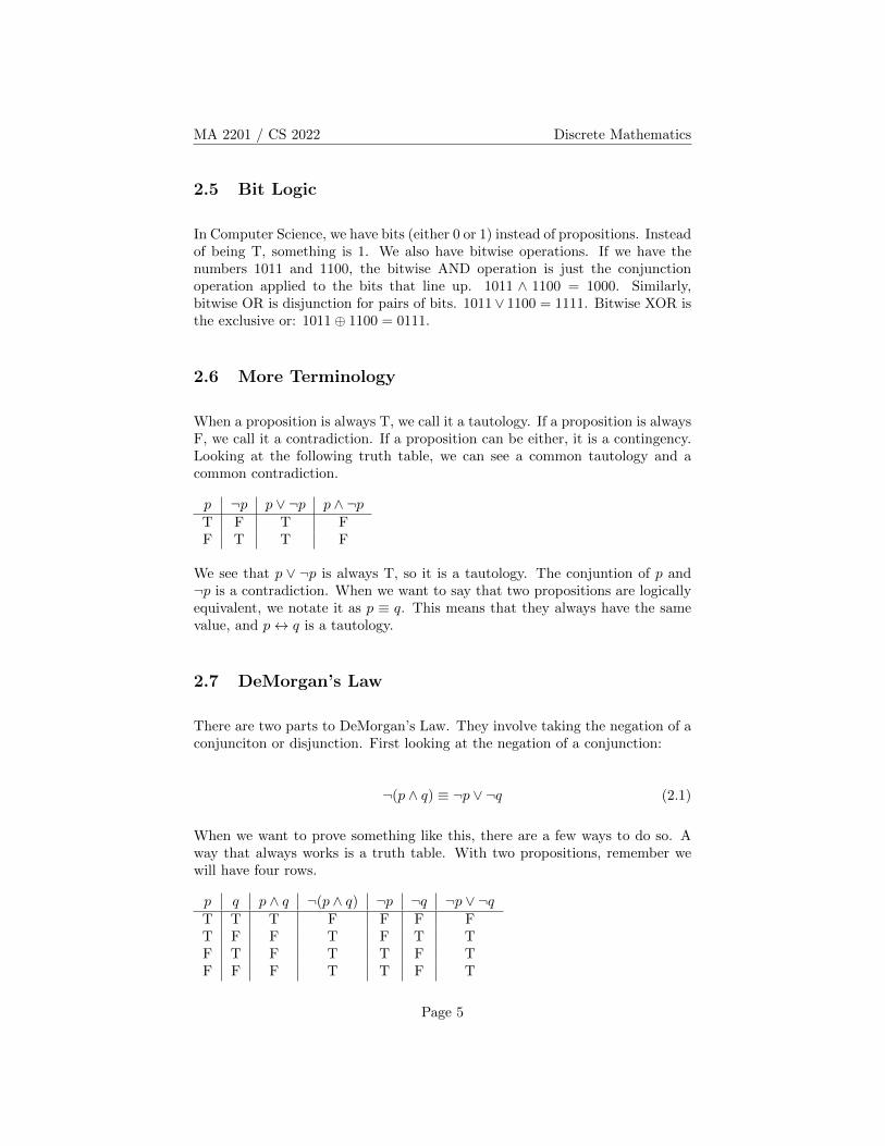
When a proposition is always T, we call it a tautology. If a proposition is alwaysF, we call it a contradiction. If a proposition can be either, it is a contingency.Looking at the following truth table, we can see a common tautology and acommon contradiction.
p ¬p p ∨ ¬p p ∧ ¬pT F T FF T T F
We see that p ∨ ¬p is always T, so it is a tautology. The conjuntion of p and¬p is a contradiction. When we want to say that two propositions are logicallyequivalent, we notate it as p ≡ q. This means that they always have the samevalue, and p↔ q is a tautology.
2.7 DeMorgan’s Law
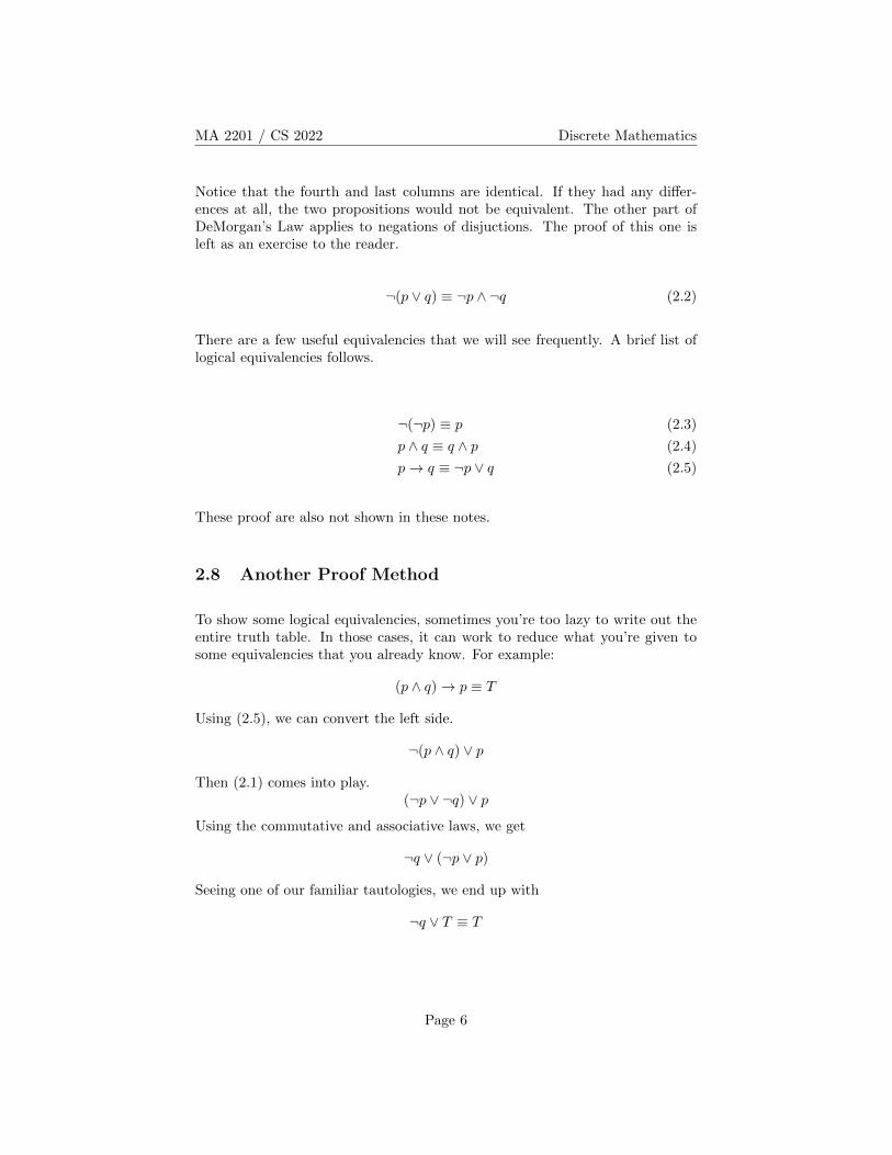
There are two parts to DeMorgan’s Law. They involve taking the negation of aconjunciton or disjunction. First looking at the negation of a conjunction:
¬(p ∧ q) ≡ ¬p ∨ ¬q (2.1)
When we want to prove something like this, there are a few ways to do so. Away that always works is a truth table. With two propositions, remember wewill have four rows.
p q p ∧ q ¬(p ∧ q) ¬p ¬q ¬p ∨ ¬qT T T F F F FT F F T F T TF T F T T F TF F F T T F T
Page 5
MA 2201 / CS 2022 Discrete Mathematics
Notice that the fourth and last columns are identical. If they had any differ-ences at all, the two propositions would not be equivalent. The other part ofDeMorgan’s Law applies to negations of disjuctions. The proof of this one isleft as an exercise to the reader.
¬(p ∨ q) ≡ ¬p ∧ ¬q (2.2)
There are a few useful equivalencies that we will see frequently. A brief list oflogical equivalencies follows.
¬(¬p) ≡ p (2.3)
p ∧ q ≡ q ∧ p (2.4)
p→ q ≡ ¬p ∨ q (2.5)
These proof are also not shown in these notes.
2.8 Another Proof Method
To show some logical equivalencies, sometimes you’re too lazy to write out theentire truth table. In those cases, it can work to reduce what you’re given tosome equivalencies that you already know. For example:
(p ∧ q)→ p ≡ T
Using (2.5), we can convert the left side.
¬(p ∧ q) ∨ p
Then (2.1) comes into play.(¬p ∨ ¬q) ∨ p
Using the commutative and associative laws, we get
¬q ∨ (¬p ∨ p)
Seeing one of our familiar tautologies, we end up with
¬q ∨ T ≡ T
Page 6
MA 2201 / CS 2022 Discrete Mathematics
3 Predicate Logic
In Predicate Logic, we are allowed to have variables. We could have a predicateP as the statement “x is greater than 3.” This gives us a function P (x) whichreturns a proposition. We call this type of function a propositional function.P (2) = F , and P (4) = T . We are allowed when doing this to have more thanone variable. We could have the predicate Q(x, y, z) : x + y = z. In this case,Q(1, 1, 2) = T and Q(1, 1, 1) = F .
3.1 Quantification
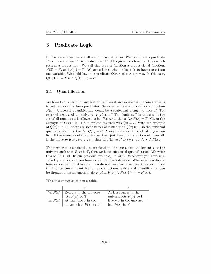
We have two types of quantification: universal and existential. These are waysto get propositions from predicates. Suppose we have a propositional functionP (x). Universal quantification would be a statement along the lines of “Forevery element x of the universe, P (x) is T.” The “universe” in this case is theset of all numbers x is allowed to be. We write this as ∀x P (x) = T . Given theexample of P (x) : x+ 1 > x, we can say that ∀x P (x) = T . With the exampleof Q(x) : x > 3, there are some values of x such that Q(x) is F, so the universalquantifier would be that ∀x Q(x) = F . A way to think of this is that, if you canlist all the elements of the universe, then just take the conjuction of them all.If the universe is x1, x2, . . . , xn, then ∀x P (x) ≡ P (x1) ∧ P (x2) ∧ · · · ∧ P (xn)
The next way is existential quantification. If there exists an element x of theuniverse such that P (x) is T, then we have existential quantification. We writethis as ∃x P (x). In our previous example, ∃x Q(x). Whenever you have uni-versal quantification, you have existential quantification. Whenever you do nothave existential quantification, you do not have universal quantification. If wethink of universal quantification as conjuctions, existential quantification canbe thought of as disjunction. ∃x P (x) ≡ P (x1) ∨ P (x2) ∨ · · · ∨ P (xn).
We can summarise this in a table.
T F∀x P (x) Every x in the universe
lets P (x) be TAt least one x in theuniverse lets P (x) be F
∃x P (x) At least one x in theuniverse lets P (x) be T
Every x in the universelets P (x) be F
Page 7
MA 2201 / CS 2022 Discrete Mathematics
3.2 A Short Review
In predicate logic, we have a predicate P (x), where individual values of x pro-vide individual propositions. We also have universal and existential quantifiers∀x P (x) and ∃x P (x). For example, consider the statement “Everyone in thisclass has taken a CS class before.” We want to turn this into predicate logic.There are often many options, and all are correct as long as they capture exactlythe logical content of the sentence. Suppose we pick the predicate P (x, y): Thestudent x in this class has taken the CS class y before. Now we want to see howto quantify P to capture the statement. We can do this by ∀x ∃y P (x, y). Forevery student, there is a CS course they’ve taken. Note that this is differentfrom ∃y ∀x P (x, y). That would say that there is a single y that satisfies P (x, y)for every x. This is called nested quantifiers, and it’s important to know thatthe order (almost) always matters.
Suppose we have the predicate Q(x, y) : x+ y = 0. Consider ∀x ∃y Q(x, y) and∃y ∀x Q(x, y). The first one is true; no matter what x we pick, we can see thatit is T when y = −x. The second one is false; no matter what y we pick, thereis at least one x for which it is F.
Now let’s consider negations of quantifiers. If we have a proposition ¬(∀x P (x)),it is equivalent to ∃x ¬P (x). Similarly, ¬(∃x P (x)) ≡ ∀x ¬P (x). The carefulreader will remember that this is basically DeMorgan’s Law, as the differentquantifiers are similar to conjunction and disjuntion. The negation of the state-ment, “At least one student in this class has taken a CS class before,” wouldbe, “Every student in this class has not taken a CS class before.”
4 Sets
A set is an unordered collection of elements. We put elements in brackets, sowe can say that S = {a, b, c}. Two sets are equal if they have exactly the sameelements, so {3, 2, 1} = {1, 2, 3}. Also, each element is either in or not in a set,so there are no duplicates. The set {1, 1, 2, 3, 3, 3} is the same as the set {1, 2, 3}.This works fine if there aren’t very many elements in the set. Some sets haveinfinitely many elements. For example, N is the set of all natural numbers.N = {0, 1, 2, . . . }. We use the dots to say that the pattern repeats forever. Wecan use them on the other side as well, as with Z = {. . . ,−2,−1, 0, 1, 2, . . . }.This is the set of integers. We can also use a set-builder notation, such asS = {x|x is an odd integer no greater than 10}. That is read as “S is the set ofevery x satisfying the property that x is an odd integer no greater than 10.”
We read the symbol ∈ as “is in the set,” so a ∈ A means that a is in the set A,
Page 8
MA 2201 / CS 2022 Discrete Mathematics
or a is an element of A. Not every set has any elements. ∅ = {} is the empty setand has no elements. If we want to compare two sets, we might want to say thatone is a subset of the other. A ⊆ B means that ∀x, x ∈ A→ x ∈ B. Rememberthat the way implication works means that ∅ is a subset of every single set. Wesometimes talk about proper subsets A ( B. This means that A ⊆ B and alsoA 6= B. Some textbooks use ⊂ instead of one of the two subset symbols, moreoften replacing (. Because that symbol is ambiguous, these notes will not useit anymore.
One important thing about sets is that A = B is the same as saying A ⊆ Band B ⊆ A. Another important thing is the cardinality. |A| is the number ofelements of A. If A is infinite, for now just say that the cardinality is infinite.We’ll get back to this later, as it’s actually quite interesting to see if an infiniteset can be bigger than another infinite set.
If we have a set A, we can talk about the power set of A, P (A). The ele-ments of P (A) are sets. This can take some effort to think about, but re-alise that a set is a thing, and anything can be an element. Specifically,the elements of P (A) are every possible subset of A. If A = {1, 2, 3}, thenP (A) =
{∅, {1}, {2}, {3}, {1, 2}, {1, 3}, {2, 3}, A
}. In this case, |P (A)| = 8. In
general, if |A| = n, then |P (A)| = 2n. For each element of A, it can either be inor not be in a given subset. That’s two choices for each element, so the productrule says that there are 2n different possible subsets.
4.1 Set Operations
There is something called the Cartesian Product of two sets. A × B is a setof ordered pairs of elements. For ordered pairs (or triplets, or more), we useparentheses rather than braces. A × B = {(a, b)|a ∈ A, b ∈ B}. For example,supposeA = {1, 2} andB = {a, b, c}. First note that the cardinality ofA×B willbe the product of the cardinalities of A and B, which in this case is 6. A×B ={
(1, a), (1, b), (1, c), (2, a), (2, b), (2, c)}
. We could also take the cartesian product
of more than two sets. A1 ×A2 × · · · ×An ={
(a1, a2, . . . , an)|ai ∈ Ai
}. In this
case, we use the shorthand ai ∈ Ai to say that a1 ∈ A1, a2 ∈ A2, . . . , an ∈ An.
Next is the union. A ∪ B = {x|(x ∈ A) ∨ (x ∈ B)}. The union of two sets isthe set containing every element in either of them. Similarly is the intersection,which corresponds with conjunction. A ∩ B = {x|(x ∈ A) ∧ (x ∈ B)}. Thisis every element in both of them. Given sets A = {1, 2, 3} and B = {1, 3, 5},A∪B = {1, 2, 3, 5} and A∩B = {1, 3}. If, for two sets A and B, A∩B = ∅, wesay that they are disjoint. If A and B are disjoint, we have |A ∪B| = |A|+|B|. Ifthey aren’t disjoint, then we need to modify this by subtracting the intersection,because the intersection was counted twice. In general, |A ∪B| = |A| + |B| −|A ∩B|. We call this the inclusion-exclusion principle.
Page 9
MA 2201 / CS 2022 Discrete Mathematics
The last operation we will discuss is the set difference operation, A − B ={x|(x ∈ A)∧ (x 6∈ B)}. If we have a universal set U , then the complement of A,denoted A, is defined as A = U −A. This is every element that is not in A.
There is a version of DeMorgan’s Law that applies to sets. One version of it isA ∩B = A∪B. We can show this sort of equivalence using membership tables,which are similar to truth tables.
4.2 A Quick Review
With sets, we talked about five operations: cartesian product (A × B), union(A∪B), intersection (A∩B), difference (A−B), and complement (A). We alsohave set identities, similar to logical equivalences. DeMorgan’s Law applies tosets in this way.
4.3 Verifying Set Identities
One way to show that two sets are equal is to show that both are subsets of theother. (A ⊆ B)∧ (A ⊇ B) ≡ A = B. Using DeMorgan’s Law as an example, wewant to show that A ∩B = A ∪ B. First we look at the ⊆ direction. Assumethat x ∈ A ∩B. This means x 6∈ A ∩ B. If it is not in the intersection, then(x 6∈ A)∨(x 6∈ B). This means (x ∈ A)∨(x ∈ B), which gives us that x ∈ A∪B.Showing the other direction is left as an exercise for the student.
Another way is a membership table. This is similar to a truth table. Ratherthan using T and F, we use I (in) and O (out). Because this is so similar, noexample will be given at this point.
A third method is to reduce the statements to propositional logic, and thenwe can show that the propositions are equivalent. Looking at DeMorgan’s Lawagain:
A ∩B ={x∣∣¬((x ∈ A) ∧ (x ∈ B)
)}(4.1)
= {x|¬(x ∈ A) ∨ ¬(x ∈ B)} (4.2)
={x∣∣(x ∈ A) ∨ (x ∈ B)
}(4.3)
= A ∪B (4.4)
Page 10
MA 2201 / CS 2022 Discrete Mathematics
4.4 Generalised Union and Intersection
If we have multiple sets A1, A2, . . . , An, we may want to look at the union of allof them. We write
A1 ∪A2 ∪ · · · ∪An =
n⋃i=1
Ai
Similarly for intersections, we write
A1 ∩A2 ∩ · · · ∩An =
n⋂i=1
Ai
For example, if we define the sets so that Ai = {i, i + 1, i + 2, . . . }, then wewould have, for any n,
⋃ni=1Ai = A1 = {1, 2, 3, . . . } and
⋂ni=1Ai = An =
{n, n+ 1, n+ 2, . . . }.
4.5 Computer Representation
If we have a universal set U = {1, 2, 3, . . . , 10}, then we can encode sets as 0− 1vectors, with 0 for something not being in the set and 1 for something being inthe set. For example, S = {1, 3, 5} would be encoded as 1010100000, where thefirst, third, and fifth elements are in S and everything else is not in S. Here,unions are done as bitwise OR, and intersections are computed as bitwise AND.
5 Functions
Functions are ways of going between sets. They take inputs from sets and returnoutputs from other (not necessarily different) sets. The statement f : A → Bmeans that f is a function, it’s input comes from the set A, and it gives anoutput in the set B. Furthermore, for every single element in A, f will assignit a single element in B. If a ∈ A, there must be a value for f(a). It can’t betwo things. Do not confuse this to mean that two elements in A can’t have thesame output. Suppose A is the real numbers (R) and B is also the real numbers.Define f(a) = 1. For every single input, there is an output (1), but each inputshares the same output. We refer to A as the domain and B as the co-domain.Also, we say b is the image of a, and a is the pre-image of b.
The set of images of a function is called the range of that function. Note that therange and co-domain do not need to be equal. Sometimes it is, and sometimesit is not. It is always true that Range(f) ⊆ Co-Domain(f).
Page 11
MA 2201 / CS 2022 Discrete Mathematics
Suppose we take f : Z→ Z to be defined as f(x) = x2. In this case, the rangeis the set {0, 1, 4, 9, 16, 25, . . . }. This is the set of perfect squares. In this case,the range and co-domain are not equal.
5.1 Special Functions
If we do not allow two different inputs to produce the same output, we callthat sort of function an injection, or a one-to-one function. If a1, a2 ∈ A anda1 6= a2, then a one-to-one function f will guarantee that f(a1) 6= f(a2). Thecontrapositive of this says that, if f(a1) = f(a2), then we are guaranteed thata1 = a2. Note that our example of f : Z→ Z with f(x) = x2 is not an injection.If we change the domain and co-domains to be the non-negative integers (Z≥0),then f becomes an injective function.
Another special function is when the range and co-domain are equal. We callthese functions surjections, or onto functions. With a surjective function, weknow ∀b ∈ B, there is at least one a ∈ A such that f(a) = b.
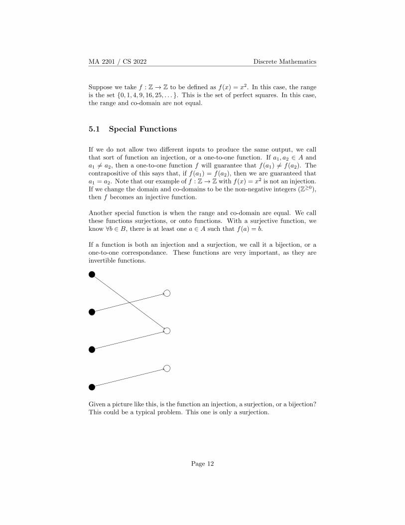
If a function is both an injection and a surjection, we call it a bijection, or aone-to-one correspondance. These functions are very important, as they areinvertible functions.
Given a picture like this, is the function an injection, a surjection, or a bijection?This could be a typical problem. This one is only a surjection.
Page 12
MA 2201 / CS 2022 Discrete Mathematics
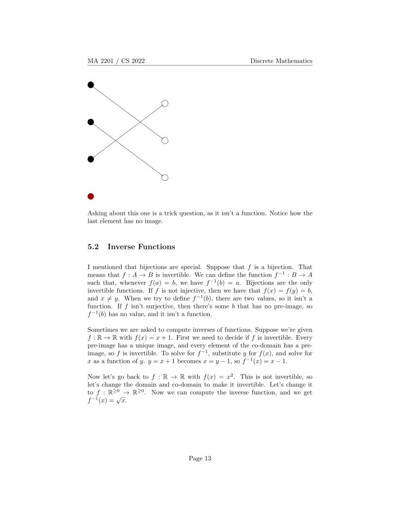
Asking about this one is a trick question, as it isn’t a function. Notice how thelast element has no image.
5.2 Inverse Functions
I mentioned that bijections are special. Suppose that f is a bijection. Thatmeans that f : A → B is invertible. We can define the function f−1 : B → Asuch that, whenever f(a) = b, we have f−1(b) = a. Bijections are the onlyinvertible functions. If f is not injective, then we have that f(x) = f(y) = b,and x 6= y. When we try to define f−1(b), there are two values, so it isn’t afunction. If f isn’t surjective, then there’s some b that has no pre-image, sof−1(b) has no value, and it isn’t a function.
Sometimes we are asked to compute inverses of functions. Suppose we’re givenf : R → R with f(x) = x + 1. First we need to decide if f is invertible. Everypre-image has a unique image, and every element of the co-domain has a pre-image, so f is invertible. To solve for f−1, substitute y for f(x), and solve forx as a function of y. y = x+ 1 becomes x = y − 1, so f−1(x) = x− 1.
Now let’s go back to f : R → R with f(x) = x2. This is not invertible, solet’s change the domain and co-domain to make it invertible. Let’s change itto f : R≥0 → R≥0. Now we can compute the inverse function, and we getf−1(x) =
√x.
Page 13
MA 2201 / CS 2022 Discrete Mathematics
5.3 A Minute Review
Special types of functions are injections and surjections. Bijections are functionsthat are both. If a function f is a bijection, it has an inverse, and
(f(a) = b
)↔(
f−1(b) = a).
5.4 Composition of Functions
If we have two functions g : A → B and f : B → C, where the range of g is asubset of the domain of f , we can define the composition (f ◦ g) : A → C as(f ◦ g)(a) = f(g(a)).
Note that the order is very important. Consider f(x) = 2x+3 and g(x) = 3x+2,where both functions have the real numbers as their domains and co-domains.(f ◦ g)(x) = f(g(x)) = f(3x + 2) = 2(3x + 2) + 3 = 6x + 7, and (g ◦ f)(x) =g(f(x)) = g(2x+ 3) = 3(2x+ 3) + 2 = 6x+ 11.
If f is invertible, then let f(a) = b. Notice that (f−1 ◦ f)(a) = f−1(f(a)) =f−1(b) = a. This is known as the identity function iA. If we switch the order,out input will be from B, but it will still be an identity function, so we call itiB .
5.5
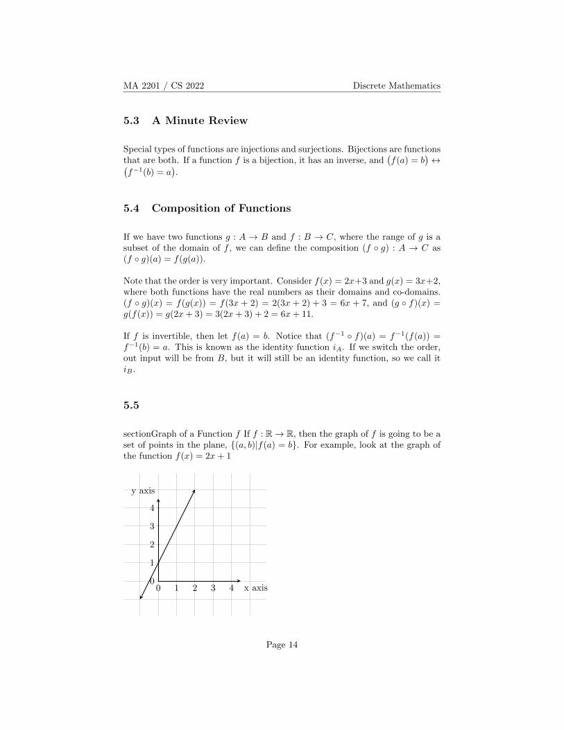
sectionGraph of a Function f If f : R→ R, then the graph of f is going to be aset of points in the plane, {(a, b)|f(a) = b}. For example, look at the graph ofthe function f(x) = 2x+ 1
x axis
y axis
0 1 2 3 40
1
2
3
4
Page 14
MA 2201 / CS 2022 Discrete Mathematics
5.6 Some special functions
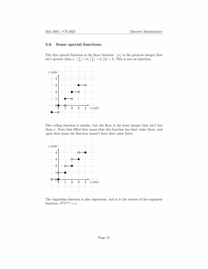
The first special function is the floor function. bxc is the greatest integer thatisn’t greater than x. b 12c = 0, b 52c = 2, b2c = 2. This is not an injection.
x axis
y axis
0 1 2 3 40
1
2
3
4
The ceiling function is similar, but the floor is the least integer that isn’t lessthan x. Note that filled dots mean that the function has that value there, andopen dots mean the function doesn’t have that value there.
x axis
y axis
0 1 2 3 40
1
2
3
4
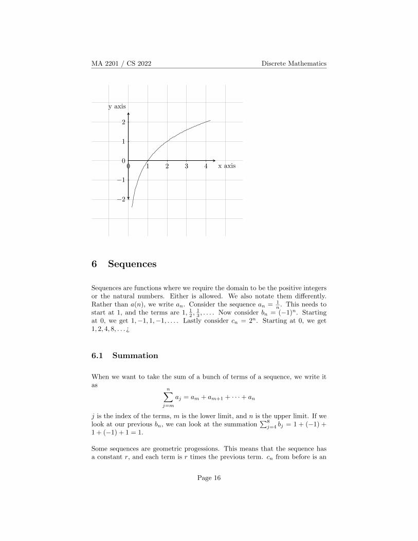
The logarithm function is also important, and it is the inverse of the exponentfunction. blogb(x) = x.
Page 15
MA 2201 / CS 2022 Discrete Mathematics
x axis
y axis
0 1 2 3 4
−2
−1
0
1
2
6 Sequences
Sequences are functions where we require the domain to be the positive integersor the natural numbers. Either is allowed. We also notate them differently.Rather than a(n), we write an. Consider the sequence an = 1
n . This needs tostart at 1, and the terms are 1, 12 ,
13 , . . . . Now consider bn = (−1)n. Starting
at 0, we get 1,−1, 1,−1, . . . . Lastly consider cn = 2n. Starting at 0, we get1, 2, 4, 8, . . . ¿
6.1 Summation
When we want to take the sum of a bunch of terms of a sequence, we write itas
n∑j=m
aj = am + am+1 + · · ·+ an
j is the index of the terms, m is the lower limit, and n is the upper limit. If welook at our previous bn, we can look at the summation
∑8j=4 bj = 1 + (−1) +
1 + (−1) + 1 = 1.
Some sequences are geometric progessions. This means that the sequence hasa constant r, and each term is r times the previous term. cn from before is an
Page 16
MA 2201 / CS 2022 Discrete Mathematics
example of this, where r = 2. For these sequences, we say that the first term isa, and the nth term is arn. There is a formula to find summations of geometricprogressions.
S =
n∑j=0
arj
rS =
n∑j=0
arj+1
Let k = j + 1
rS =
n+1∑k=1
ark
rS = S + arn+1 − a
S =arn+1 − ar − 1
For example,∑n
j=0 2j = 2n+1 − 1.
6.2 Double (or Triple (or More!)) Summation
We can also write summations inside of other summations. When we write∑3i=0
∑4j=1 ij, then we first evaluate the inner-most summation. This gives us∑3
i=0(i+ 2i+ 3i+ 4i) =∑3
i=0 10i = 10∑3
i=0 i = 10(0 + 1 + 2 + 3) = 60.
7 Cardinality of Sets
When sets are finite, their cardinalities are rather boring. It’s way more funwhen they’re infinite. However, some things work regardless of whether or notthey are infinite. If, for sets A and B, there exists a bijection f : A → B,then we say that |A| = |B|. For examples, we’re only go to use infinite sets,because otherwise it’s pretty boring. Consider the sets N>0 = {1, 2, 3, . . . }and O>0 = {1, 3, 5, . . . }. Consider the funciton f : N>0 → O>0 defined asf(x) = 2x−1. Try to convince yourself this is a bijection for a reason other than,“Professor Sarkozy posted these notes and probably made sure they’re correct.”Once you decide it’s a bijection, you know that
∣∣N>0∣∣ =
∣∣O>0∣∣. This cardinality
is a famous cardinality referred to as ℵ0. A set with the same cardinality asthe positive integers is countably infinite. A set is called countable if it is eitherfinite or countably infinite.
Page 17
MA 2201 / CS 2022 Discrete Mathematics
It can be difficult to show that the rational numbers are countably infinite, butit is nevertheless true. Something we will show next is that |N| < |R|.
7.1 A Pithy Review
The smallest infinity is the countable infinity, ℵ0 = |N| = |Z| = |Q|. A proof forQ being countable is in the book. To show that something is countably infinite,we have to list the elements of the set so we list everything exactly once. Theclear question is, “Is there a set that is not countably infinite?”
7.2 Continuum Cardinality
We define c := |R|. It turns out that |R| = |P (N)| = 2ℵ0 . What we will firstshow is that the set of real numbers between zero and one, R(0,1), is uncountable.We will use the Cantor diagonalization technique. The technique shows thatany possible listing of the real numbers between zero and one will fail to includesomething. We will use a proof by contradiction.
Assume we have a listing of R(0,1). We will construct a real number ∈ (0, 1)that is not on the list. For our listing, we will use a decimal representation ofthe numbers. Each number will have infinitely many digits. If it notmally hasa finite representation, we just add zeros to the end. Suppose, for the sake ofexample, that our listing is as follows:
1→ .2347 . . .
2→ .3510 . . .
3→ .2445 . . .
...
i→ . . . aii
Look at the main diagonal: the ith digit of the ith number on the list. Thisgives us 2, 5, 4, . . . , aii. Construct a number that matches none of these, such as0.545 . . . We can define this formally by saying that the ith digit, di, is 5 whenaii 6= 5 and 4 otherwise. Five and four are not special, but be sure to not usezero and nine, because those get weird.1 Call this number x. We know that x
1You may remember some weird kid in middle school trying to convince you that0.999999 · · · = 1. Or maybe they were trying to convince you the opposite (in which casethat strange kid was wrong). Any number with a finite decimal representation has a secondrepresentation which is infinite and ends with infinitely many nines. To avoid this, we don’tallow di to ever be 0 (to prevent finite representations) or 9 (to prevent infinitely many nines).These representations would not be on the list, but they might match something on the list.
Page 18
MA 2201 / CS 2022 Discrete Mathematics
can’t be the first element of the list, because it has the wrong first digit. It alsocan’t be the second, because the second digit is wrong. In fact, it can’t be theith element, because it doesn’t match that. So x can’t be any element on thelist, so it was forgotten. But we could do this with any listing of real numbers,so there is no listing that has everything.
So the cardinality of the reals is greater than ℵ0. In fact, if we use binaryrepresentations of numbers, we can see that infinitely many digits gives us 2ℵ0
possible values, so ℵ0 < 2ℵ0 . In fact, this can continue, as 2ℵ0 < @2ℵ0 . Thereare infinitely many infinite cardinalities which can be constructed this way. Ifwe have a list of every cardinality, ℵ0 < ℵ1 < ℵ2 < · · · , we want to know if it istrue that ℵ1 = 2ℵ0 = c. According to a popular hypothesis called the continuumhypothesis, the equality is true. The most common axiom system, the ZermelloFraenkel axiom system, it is proven that the statement can be neither provednor disproved; it is undecidable. Not that it is relevant to this course, but ithas been shown that every set of axioms will have undecidable questions, andthis caused a lot of controversy when it was proven.
8 Algorithms
An algorithm is a definite procedure that solves a problem in a finite numberof steps. It cannot be random, and it has to terminate for any input. We can’tloop forever. Algorithms are given input, they produce output, and every stepneeds to be well-defined. We like it when each step can be done efficiently.
Our first example will be an algorithm that finds the maximum of a list ofn numbers, a1, a2, . . . , an. For example, with an input of 3, 1, 5, 4, we shouldreturn 5. Our algorithm will look at each element of the list in order. It alsokeeps track of the maximum value so far (temporary maxmimum). When itlooks at a number, if that number is greater than the temporary maximum, itchanges the value of the temporary maximum to the new number. After lookingat each element, the maximum is the value of the temporary maximum.
Step 1 Set the temporary maximum to a1.
Step 2 Compare temporary maximum to the next number. If the next numberis greater, we set the temporary maximum to this new number.
Step 3 Repeat Step 2 until we have no numbers left.
Step 4 Output the temporary maximum.
Page 19
MA 2201 / CS 2022 Discrete Mathematics
Now we can write it in pseudocode (remember how this is a CS course?).
max := a1
for i = 2 to n
if max < ai then max := ai
rof
return max
Next is the search problem. As input, we are given a number x and a lista1, a2, . . . , an. The output is i if x = ai or 0 if x 6∈ {a1, a2, . . . , an}. We willlook at linear search.
i := 1
while (i ≤ n) ∧ (x 6= ai)
i := i+ 1
elihw
if i ≤ n then return i
else return 0
Now suppose we are guaranteed to have a sorted list. There is a more efficientalgorithm called binary sort. We look at the middle element of the list. Withthis one comparison, we can elimate half of the list.
i := 1, j := n
while (i < j)
m := b i+ j
2c
if x > am then i := m+ 1
else j := m
elihw
if ai = x then return i
else return 0
In this, i and j represent the current search interval. Each time through the loop,we stop looking at half of the list, so the search interval will shrink. Eventuallyit will be a single element. We haven’t yet talked about complexity, but thisone is significantly more efficient.
8.1 A Concise Review
Some algorithms are generally accepted to be better than others. This is usuallybecause of either time complexity or space complexity. In CS 2223, you can learn
Page 20
MA 2201 / CS 2022 Discrete Mathematics
about both. In this class, we’ll only talk about time.
8.2 Time Complexity
The time complexity of an algorithm is the number of basic operations per-formed. In this course, comparisons are basic operations.
Commonly, we only consider the worst-case time complexity and the averagetime complexity. The worst-case is the most number of basic operations forany possible input. The average is an average over every possible input. We’lluse the three previous algorithms and compute their time complexities. In thisclass, we count loop comparisons when looking at the number of comparisons.
8.2.1 Maximum
For Maximum, We start by assigning a value to the temporary maximum. Thishas no comparisons. Inside our loop, we have two comparisons: we check that iis less than n, and we compare the temporary maximum to ai. That comes totwice n− 1 comparisons, plus an extra comparison once i = n+ 1 to break outof the loop. After that, we have no more comparisons. So the total number ofcomparisons is 2(n− 1) + 1 = 2n− 1.
8.2.2 A Short Sidetrack
When we talk about complexities, it helps to talk about the growth of functions.We will introduce “Big Oh notation”. When we talk about O(f(n)), we don’tcare about constants. We only care about the core growth of the function. Theprecise definition compares two functions f and g. Colloquially, f = O(g) if fgrows slower than g (or at the same speed). Formally, f = O(g) means thatsome constants c and k exist such that |f(x)| ≤ c |g(x)| whenever x > k. Thatis, whenever x is big enough, f is smaller than some constant times g.
Consider the function f(x) = x2 + 3x+ 1. We want to know which term is mostimportant, and which are lesser terms. If we set k = 1, then we only need to lookat this function when x > 1. Then that happens, f(x) ≤ x2 + 3x2 + x2 = 5x2.Now we can say that c = 5 and g(x) = x2. Whenever x > 1, f(x) ≤ 5g(x). Now,it’s also true that f = O(x3), but that is a looser bound, so it is more useful tosay that f = O(x2). In fact, for any nth-order polynomial h(x), h = O(xn).
Page 21
MA 2201 / CS 2022 Discrete Mathematics
8.2.3 Linear Search
Going back to our previous algorithms and their time complexity, let’s lookat Linear Search. Here, we start by assigning a value for i. Then we do twocomparisons for each i until we stop. For this algorithm, it matters whether ornot x is in the list. For now, let’s assume that x = aj . We will have j valuesfor i, giving us 2j comparisons. Outside of the loop, we do one comparison tosee if i ≤ n. This comes to a total of 2j + 1 comparisons. The number of thesecomparisons is any of {3, 5, . . . , 2n+ 1}. Now assume that x 6∈ {a1, a2, . . . , an}.This goes through the loop n times for 2n comparisons. Then it does the firstloop comparison when i = n+ 1 and breaks the loop. Lastly it checks if i ≤ n,for a total of 2n+ 2 comparisons. This is the worst case, and 2n+ 2 = O(n) islinear. We’ll come back to the average case later.
8.2.4 Binary Search
For this algorithm, we cut in half the search interval each time through theloop. Each time through the loop is two comparisons (i < j and x > am). Thenthere’s one comparison to break the loop and one comparison to see if we foundx. So with p splits, we have 2p + 2 comparisons. If we assume that n = 2k,then after k splits, i and j will be equal. That means that k = log2(n). Thecomplexity of this algorithm is 2 log2(n) + 2 = O(log(n)). It turns out that,when using Big Oh notation, we don’t need to specify the base of the logarithm.The base of the logarithm is just a constant factor.
Now suppose 2k < n < 2k+1. In this case, k = blog2(n)c. We can expand thelist to have 2k+1 elements, and the search will take 2blog2(n)c+ 4 comparisons,which isn’t significantly worse.
8.2.5 Average Case
For an example of average case complexity, let’s look back at linear search.For simplicity, we’ll assume that x is in the list. The possible numbers ofcomparisons are {3, 5, . . . , 2n + 1}. To compute the average, we just add them
Page 22
MA 2201 / CS 2022 Discrete Mathematics
all up and divide by n, the number of possibilities.
3 + 5 + · · ·+ 2n+ 1
n
=2(1 + 2 + · · ·+ n) + n
n
=n(n+ 1) + n
n=n+ 2
Between the second and third rows, we used an identity that we’ll prove laterin the course for the sum of the first n numbers.
9 Number Theory
Number theory is the study of the positive integers. One of the most importantthings is divisors. We say that a is a factor of b (a | b) if there is an integer csuch that ac = b. For examples, 3 | 6 and 3 - 7. This has some properties. Ifa | b and a | c, then a | b+ c. If a | b, then a | bc. Lastly, if a | b and b | c, thena | c.
9.1 Primes
Using this operation, we can define primes. A number p is prime if a | p is onlytrue when a = 1 or a = p. We don’t consider 1 to be a prime number.
9.2 A Condensed Review
Primes are numbers with exactly two divisors: one and themselves.
9.3 Fundamental Theorem of Arithmetic
The Fundamental Theorem of Arithmetic (big name probably means important)says that every positive integer other than 1 can be written uniquely as a productof primes, when the primes come in increasing order. This is called the primefactorization of a number. For example, the prime factorization of 100 is 2 ·2 · 5 · 5 = 2252. At the moment, we have no efficient way to find the primefactorization of a number, and this is the basis for RSA encryption.
Page 23
MA 2201 / CS 2022 Discrete Mathematics
The greatest common divisor of two numbers, gcd(a, b) is the largest integer dsuch that d | a and d | b. If we have the prime factorization of both numbers,it is easy to find the greatest common divisor. For example, we’ll computegcd(12, 20). 12 = 22 · 3 and 20 = 22 · 5. The only prime factor they share is2, and they both have 22 as a factor, so gcd(12, 20) = 4. In general, we takethe common prime factors, and, for each such prime, we take the smaller of theexponents. Unfortunately, we often don’t have the prime factorizations, so weneed other ways to compute the greatest common davisor in practice.
The least common multiple of two numbers lcm(a, b) is the smallest integer dsuch that a | d and b | d. For example, we’ll again use 12 and 20. For this,we take each prime factor of either and use the larger exponent. lcm(12, 20) =22 · 3 · 5 = 60.
10 Writing Proofs
Now that we have a bunch of definitions, we’d like to prove some things. To dothis, we need to know the rules of inference, which are the steps we’re allowedto take.
10.1 Rules of Inference
(1) Modus ponens: If we already know p→ q and we also know p is true, we candraw the conclusion that q is true. For example, we know that if today isThursday, we have CS 2022 today. We also know (at the time of this lecture)that today is Thursday. ∴ (that symbol means therefore) we have CS 2022today. This rule of inference is similar to the tautology: ((p→ q) ∧ p)→ q.
(2) Modus tollens: If we know p → q and q is false, we can conclude p is false.For example, we know that If today is Saturday, we don’t have CS 2022today. We also know that we have CS 2022 today. ∴ today is not Saturday.This is similar to the tautology: ((p→ q) ∧ ¬q)→ ¬p.
(3) Simplification: If we know p∧q, we also know p is true. Because conjunctionis commutative (p ∧ q is the same as q ∧ p), we also know q is true.
(4) Addition: If we know p, we also know p ∨ q. Again, this is rather simple.
(5) Hypotheical syllogism: If we know p → q and q → r, we are allowed toconclude p→ r (which you may remember from homework 1).
(6) Disjunctive syllogism: If we know both p ∨ q and p is false, we can deducethat q is true. Again, like with Simplification, we can swap p and q here.
Page 24
MA 2201 / CS 2022 Discrete Mathematics
(7) Conjunction: If we know both p and q are true, we know that p ∧ q is true.This is again rather straightforward.
(8) Resolution: This one is a bit trickier. If we know both p ∨ q is true and¬p∨ r is true, we can say that q∨ r is true. This is because either p or ¬p isfalse, and the other term in whichever disjunction the false one is in mustbe true.
(9) Dilemma (proof by cases): If we know p1 → q and p2 → q, and we alsoknow p1 ∨ p2 is true, then we can say q must be true.
These steps are all valid. There are also some steps people often think areallowed but are not. These are called the fallacies, or invalid steps.
10.2 Common Fallacies
(1) Fallacy of affirming the conclusion: If we know that p → q and that q istrue, it is invalid to conclude that p is true.
(2) Fallacy of denying the hypothesis: If we know that p→ q and that p is false,it is invalid to conclude that q is false.
(3) Fallacy of begging the question (circular reasoning): In this fallacy, withinour argument, we assume that the statement we are trying to show is true.If we’re trying to prove a theorem, it is invalid to use that theorem in ourproof.
That last one warrants an example. The following is not a valid proof. Wewould like to show that, if n2 is even, then n is even. Assume that n2 is even.This means n2 = 2k for some integer k. Now let n = 2l for some l. Because n istwice l, n is an even number, and we have finished what we are trying to show.
10.3 Examples of These Rules
On an exam, you might be given an inference and asked if it is valid. Here aresome examples.
10.3.1 Example 1
If the last digit of a number n is 0, then 10 | n. The last digit of 910 is 0. ∴10 | 910. This is valid, and it is modus ponens.
Page 25
MA 2201 / CS 2022 Discrete Mathematics
10.3.2 Example 2
If x is even, then x(x+ 1) is even. If x is odd, then x+ 1 is even and x(x+ 1)is even. x is either even or odd. ∴ x(x + 1) is odd. This is valid, and it is adilemma.
10.3.3 Example 3
If Ben cheats, then he sits in the back row. Ben sits in the back row. ∴ Bencheats. This is invalid. Not everyone who sits in the back row is a cheater. Thisis the fallacy of affirming the conclusion.
10.3.4 Example 4
If it snows today, the university will close. The university did not close today.∴ it did not snow today. This is valid, and it is modus tollens.
10.3.5 Example 5
If n > 2, then n2 > 4. n ≤ 2. ∴ n2 ≤ 4. This is invalid, and it is the fallacy ofdenying the hypothesis.
10.4 A Succinct Review
In this class, learning to prove theorems is very important. We use rules ofinference to be able to prove things. However, we still don’t quite have all therules we’d like to use, so we’ll look at some more.
10.5 Quantified Rules of Inference
These rules of inference all apply to quantified predicates.
(1) Universal instantiation: ∀xP (x) ∴ P (c) If we know that something is truefor every x, we can plug in a c and it is true.
Page 26
MA 2201 / CS 2022 Discrete Mathematics
(2) Universal generalization: P (c) for any c ∴ ∀xP (x) If we know something istrue for any arbitrary c, we can say it is true for every x.
(3) Existential instantiation: ∃xP (x) ∴ P (c) for some c If there exists an x tosatisfy P (x), we can let c be that value.
(4) Existential generalization: P (c) for some c ∴ ∃xP (x) If we found a c tosatisfy P (c), then there exists a value of x to satisfy P (x).
(5) Universal modus ponens: ∀x(P (x) → Q(x)), P (c) ∴ Q(c) This is a combi-nation of both modus ponens and universal instantiation.
(6) Universal modus tollens: ∀x(P (x)→ Q(x)), ¬Q(c) ∴ ¬P (c) This is a com-bination of both modus tollens and universal instantiation.
10.6 What is a Proof?
When proving, there is a theorem we are trying to prove. The argument we useis the proof. Within the proof, we sometimes show smaller results that help toprove the theorem. We call these lemma. A corollary is a similar result to thetheorem that we show after the proof. A conjecture is something we think istrue, but we have no proof yet.
Something that is considered by some to be unfortunate and by others to bebeautiful is that there is no algorithm for finding proofs. Proving things cantake creativity.
10.6.1 Twin-Prime Conjecture
This is an open problem for which nobody has been able to come up with aproof. Also nobody has been able to disprove it. We know that there areinfinitely many primes. We call two primes p and q twin primes if p + 2 = q.Some examples are (3, 5), (5, 7), (11, 13). The twin-primes conjecture states thatthere are infinitely many pairs of twin primes.
10.7 Some Proof Techniques
Many proofs are of the form p → q. They want to show that, when certainrequirements are true, there is a useful result that is also true. The first andsimplest proof technique is the direct proof. We assume that p is true and wetake steps to show that q is also true.
Page 27
MA 2201 / CS 2022 Discrete Mathematics
For example, consider the theorem that if n is odd, then n2 is also odd. Assumethat n is odd. We can write n = 2k + 1 for some k. n2 = 4k2 + 4k + 1 =2(2k2 + 2k) + 1. Since n2 can be written as twice an integer plus one, n2 mustbe odd.
The second proof method is the vacuous proof method. This again works for animplication. The goal is to show that p is always false (p is a contradiction). Inthis case, the implication is true, and the theorem has been proven (but is alsopretty useless).
The third proof method is the trivial proof method. If you can prove that q isalways true (q is a tautology), the the implication is always true.
Next is the indirect proof technique. This can work not only for implications.In an indirect proof, we prove something else, and then show that it gives uswhat we want. This comes in two forms: proof by contraposition and proof bycontradiction.
In a proof by contraposition, we need to be proving an implication. In this case,rather than proving p → q, we prove ¬q → ¬p, which is the contrapositive.Even though a proposition and its contrapositive are equivalent, it is sometimeseasier to prove the contrapositive. For example, consider the theorem that if n2
is even, then n is even. A proof by contraposition will show that if n is not even(if n is odd), then n2 is not even (n2 is odd). A proof of this is above. I couldcopy and paste it here, and I’d only add a line or two for this proof to point outhow they’re contrapositives.
In a proof by contradiction, we don’t require that we’re trying to prove animplication. We want to prove some proposition p. We start by assuming thetheorem is false. We assume ¬p. This is an indirect assumption. From thisassumption, we arrive at a contradiction (often q ∧ ¬q). Because we arrived ata contradiction, our assumption must be false, and this proves p.
We will show two famous theorems using indirect proofs. Specifically, we’ll useproofs by contradiction. The first is the theorem that
√2 is irrational. The
second is that there are infinitely many primes. For the first, we will assumethat
√2 is rational, and can be written as
√2 = a
b where a and b are integers.For the second, we’ll assume that there are finitely many primes. Specifically,that there is some integer k such the only primes are p1, p2, . . . , pk.
10.8 A Crisp Review
We’re trying to take a statement and come up with a rigorous proof that thestatement is correct. This can be very difficult. There are many open problems
Page 28
MA 2201 / CS 2022 Discrete Mathematics
for which nobody has found a proof. Some techniques we have for proving thingsare direct proofs, vacuous proofs, and trivial proofs. We also have indirectproofs, which can either be proofs by contraposition or proofs by contradiction.The former is one in which we prove the contrapositive of our statement (whichonly works when our statement is an implication). The latter is when we assumeour statement is false and from that prove a contradiction (often of the formp ∧ ¬p).
10.9√2 is Irrational
We will show this using a proof by contradiction. Our indirect assumption isthat
√2 is rational. This means
√2 = a′
b′ , where a′ and b′ are some integers. Wewould like to say that the gcd of the numerator and denominator is 1. Definea := a′
gcd(a′,b′) and b := b′
gcd(a′,b′) . This lets us cross out the common factors and
write√
2 = ab . This means that the numerator and denominator are relatively
prime (gcd(a, b) = 1). Now we square both sides. 2 = a2
b2 , which can be writtenas 2b2 = a2. This tells us that a2 is even. As we’ve shown previously, whenthe square of an integer is even, the integer itself is also even, so a is even. Soa = 2k, for some integer k. So 2b2 = (2k)2 = 4k2, and b2 = 2k2. This requiresb2 to be even, which requires b to be even. If both a and b are even, then theyshare a factor of 2, and gcd(a, b) 6= 1. If gcd(a, b) = 1 and gcd(a, b) 6= 1, we havea contradiction ( ). Thus, our indirect assumption must be false, as it led toa contradiction. So
√2 is irrational. We have finished our proof, so we draw a
black square. �
10.10 There are Infinitely Many Prime Numbers
We will also show this using a proof by contradiction. WAe assume indirectlythat there are finitely many prime numbers. Specifically, we have exactly kprimes, for some integer k. We can write the sequence of prime numbers asp1, p2, . . . , pk. Consider the number x = p1p2 · · · pk + 1. From the fundamentaltheorem of arithmetic, x has a prime factorization. Take one of the primesin the factorization of x and call it p. We have p | x. Because p is a prime,p | x − 1, because x − 1 is the product of every prime number. This impliesp | (x) − (x − 1), or p | 1. Because p is a prime, p ≥ 2, so p - 1. We arrivedat a contradiction, so our assumption must be false. Thus, there are an infinitenumber of prime numbers. �
Page 29
MA 2201 / CS 2022 Discrete Mathematics
10.11 Proof by Cases
To prove a dilemma p1∨p2 → q, we need to show each case: p1 → q and p2 → q.Consider this example. If 3 - n, then n2 = 3k + 1. We use the notation a ≡ bmod m to mean that a is congruent to b modulo m. This means that m | (a−b).We can rewrite the statement as: If n 6≡ 0 mod 3, then n2 ≡ 1 mod 3. Thiscan be broken into two cases. In the first case, n2 ≡ 1 mod 3. In the secondcase, n2 ≡ 2 mod 3. Consider first the former. Assume n ≡ 1 mod 3. Thenn = 3k+1 for some k. n2 = (3k+1)2 = 9k2+6k+1 = 3(3k2+2k)+1, so n2 ≡ 1mod 3. Now consider the second case. Assume n ≡ 2 mod 3, so n = 3k + 2,for some k. This means n2 = (3k + 2)2 = 9k2 + 12k + 4 = 9k2 + 12k + 3 + 1 =3(3k2 + 4k + 1) + 1, so n2 ≡ 1 mod 3. We have shown both cases, so ourstatement is true. �
10.12 Proving a Biconditional
A lot of theorems in mathematics are of the form, p is true if and only if (iff) q istrue (p↔ q). To do this, we need to prove both p→ q and also q → p. Together,these two proos will prove the biconditional. For each of these sub-proofs, wecan use any of our proof techniques. Let’s consider the statement, n is odd iffn2 is odd. First we will show that n is odd → n2 is odd. We will do this with adirect proof (which also exists ealier in these notes). We can write n = 2k + 1for some integer k. n2 = (2k + 1)2 = 4k2 + 4k + 1 = 2(2k2 + 2k) + 1, so n2 isodd. Next we show that n is odd ← n2 is odd. In this direction, we will use anindirect proof, specifically a proof by contraposition. This becomes n is even→n2 is even. We can write n = 2k, for some integer k. n2 = (2k)2 = 4k2 = 2(2k2),so n2 is even. Thus, n2 is odd → n is odd, and our second direction has beenproven. �
10.13 Multiple Biconditionals
Sometimes we want to prove that several statements are equivalent. Supposewe wish to prove p1 ↔ p2 ↔ · · · ↔ pk. Rather than proving every pair inevery direction, we will prove a circle of implications. p1 → p2, p2 → p3, · · · ,pk−1 → pk, and pk → p1.
10.14 Proving Quantified Theoresms
When we have quantified predicates, we often want to prove that they arecorrect. Remember that we have universal quantifiers ∀xP (x) and existential
Page 30
MA 2201 / CS 2022 Discrete Mathematics
quantifiers ∃xP (X). We will first talk about existential quantifiers. We havetwo methods for this. The first method finds or constructs an example of xthat makes P (x) true. This is a constructive proof. The other method is moredifficult to use, as it proves that an example must exist, but provides no way tofind it. This is a nonconstructive proof.
Going back to the sequence of prime numbers, we will use a constructive proofto show that there are arbitrarily large gaps between consecutive primes. If yougive me a large number, such as 100, I can show you 100 consecutive numberssuch that none of them are prime. Even if you give me 1, 000, 000, I can do thesame thing. However, I won’t show you how to do this until next time.
10.15 A Small Review
We need more methods for proving quantified theorems. We will start withexistential quantifiers. We can either do this by constructing an example or byshowing that an example must exist without finding it.
For every natural number n, there exist n consecutive compositie (non-prime)numbers. That is, in the sequence of prime numbers, there is a gap of at leastn, no matter what n is chosen. Consider the number x = 1 + (n + 1)! =1 + (n+ 1) · n · (n− 1) · · · 2 · 1. Consider also the numbers x+ 1, x+ 2, . . . , andx+ n. Note that x+ 1 = 2 + (n+ 1)!, so 2 | x+ 1. Also, x+ 2 = 3 + (n+ 1)!,so 3 | x + 2. In fact, x + k = (k + 1) + (n + 1)!, so (k + 1) | x + k. So these nnumbers are all composite numbers. �
In the case where n = 4, we would find x = 121, and the numbers 122, 123, 124,and 125 are all composite. Note that there is a smaller sequence of numberssatisfying this. For example, 121 = 112, so 121, 122, 123, 124 is another sequence.
An arithmetic progression is a sequence of number a1, a2, . . . , an such that ai−ai−1 = d for some constant number d. There is a theorem named the Green-Tao theorem that says the sequence of primes has arbitrarily long arithmeticprogressions. That is, for any n, there exists a set of n prime numbers thatform an arithmetic progression. This is a very new result, and the proof is quiteinvolved. It’s just something interesting to think about.
To show a nonconstructive proof, consider the statement: For every n, thereexists a prime p such that p > n. Consider the number x = n! + 1. Bythe fundamental theorem of arithmetic, x has a prime factorization. Let p bea prime divisor of x. From the same steps we used to prove that there areinfinitely many primes, we can show that no integer between 2 and n will dividex. Since p divides x, p > n.
Page 31
MA 2201 / CS 2022 Discrete Mathematics
10.16 Proving Universal Quantifiers
If we want to show something of the form ¬∀xP (x), all we need to do is finda single counter-example: a value for x for which the cnojecture is not true.Notice that this is the same as proving ∃x¬P (x), and then we’re proving anexistential quantifier. Consider the statement that every prime number is odd.We can prove the negation of this statement by pointing out that 2 is an evenprime.2 If we our universe is the natural numbers, there is a proof method calledinduction.
In induction, we have two steps. First is the basis step, where we prove thatP is true for the smallest value it’s true for. Usually 1 or 0, but sometimes 2or something else, based on the problem. Next is the inductive step. In theinductive step, we show that ∀n
(P (n) → P (n + 1)
). This, together with the
basis step, proves that P is true for every n. This is sort of like an infinitenumber of applications of modus ponens. If we know P (1) and P (1) → P (2),then we know P (2). Next we have P (2) and P (2) → P (3), so we have P (3).This continues forever, so we know it is true for every n. You can also thinkof this as an infinite sequence of dominoes. If you topple the first one, it willtopple the next one, and that will get the one after, and so on until they haveall toppled. Note that this is not circular reasoning, because we are provingan implication rather than proving P (n + 1). We will eventually also look atsomething called strong induction,3 which proves a slightly different implication.Here are some examples of induction.
We want to prove that ∀n,∑n
i=1 i = n(n+1)2 . The basis step is to show that
P (1) is true. Clearly, 22 = 1, and we are happy. Now we want to show that the
implication P (n)→ P (n+1) is true. To do this, we will assume that P (n) is true,and we’ll use a direct proof to show that P (n+1) is true. Our assumption, which
we call the inductive hypothesis, is that, for some n,∑n
i=1 i = n(n+1)2 . Notice
that∑n+1
i=1 i = n(n+1)2 + n+ 1. Moving around terms, we get n(n+1)
2 + n+ 1 =n(n+1)+2(n+1)
2 = n2+n+2n+2)2 = n2+3n+2
2 = (n+1)(n+2)2 = (n+1)((n+1)+1)
2 , andwe’re happy. By induction, we know that this formula is true for every naturalnumber n.
Now we will show that ∀n, n < 2n. Our basis step is to show that P (1) is true.1 < 2, so that’s done. Now for the inductive step. Suppose that, for some n,n < 2n. When we want to compare n + 1 and 2n+1, we can break the latterinto 2n + 2n. We know that n < 2n, and we know that 1 < 2n, and sums willpreserve the inequality, so n+ 1 < 2n+1. �
2But doesn’t that make it rather unusual, or odd?3This name is confusing, because it is a mathematically weaker proof than normal induc-
tion.
Page 32
MA 2201 / CS 2022 Discrete Mathematics
Now for an incorrect application of induction. Consider the statement that ∀n,2 | (3n − 2). Assume that this is true for some n. 3n+1 − 2 = 3(3n) − 2 =2(3n) + (3n − 2). By our inductive hypothesis, the second summand is even.Clearly the first summand is even, so the sum is even, and we’ve proven theinductive step. Unfortunately, we never proved a basis, so we haven’t proventhe statement. It turns out that this is not true for any n, so we can’t possiblyprove the basis step.
10.17 A Hasty Review
Whenever we have a statement we want to show for every natural number n(∀nP (n)), we can use induction. With induction, we prove a basis case when n isa small number (usually 1 or 0). Then we prove the implication P (n)→ P (n+1).This proves the statement.
Recall our formula for sums of geometric series.∑n
j=0 a · rj = a·rn+1−ar−1 . We
can prove this by induction as well. First we consider the case when n = 0.
a · r0 = a, and a·r1−ar−1 = a. Now we want to prove the implication in the
inductive step. We assume that∑n
j=0 a · rj = a·rn+1−ar−1 for some value of n.∑n+1
j=0 a · rj =∑n
j=0 a · rj + a · rn+1 = a·rn+1−a+a·rn+2−a·rn+1
r−1 = a·rn+2−ar−1 . So
the implication is true. The implication plus the basis case proves the theoremfor all n.
10.18 Strong Induction
This is supposedly a stronger version of induction. It is actually an equivalentproof, but it is sometimes easier to prove the implication. Here, we have the samebasis step. The basis step is the same as in regular induction. The inductivestep is different. The inductive step proves the implication
(P (1)∧P (2)∧ · · · ∧
P (n))→ P (n + 1). If you basis step is something other thatn proving P (1),
then this will impact the inductive step. If your basis step proves P (2), theinductive step will take the conjunction starting from P (2).
Recall the fundamental theorem of arithmetic. For every natural number n ≥ 2,there exists a unique prime factorization of n, where the primes are increasing.This requires both a proof of existence and a proof of uniqueness. We’ll lookfirst at existence. Our basis step in this case is P (2). The prime factorizationof 2 is simply 2, so it exists. In the inductive step, we assume that for every kin 2 ≤ k ≤ n, there exists a prime factorization for k. We want to show thatn + 1 has a prime factorization. This has two cases. Consider first the casewhen n+ 1 is a prime. In this case, it’s prime factorization is simply n+ 1. In
Page 33
MA 2201 / CS 2022 Discrete Mathematics
the second case, n + 1 has a divisor a (other than 1 or n + 1), and there’s anumber b such that ab = n+ 1. Both a and b are between 2 and n, so they haveprime factorizations. Write them as a = p1p2 · · · pk and b = q1q2 · · · ql. A primefactorization for n+ 1 is n+ 1 = ab = p1p2 · · · pkq1q2 · · · ql, so n+ 1 has a primefactorization.
Now let’s look at uniqueness. This will be a proof by contradiction. Assumeindirectly that, for some n, there are two distinct prime factorizations. n =p1p2 · · · pk = q1q2 · · · ql. We can simplify by crossing off the common primes.Assume4 that we’ve already done this, and all the primes pi are distinct fromall the primes qj . Because p1 | n, p1 | q1q2 · · · ql. Since q1q2 · · · ql can’t bedecomposed any further, p1 must divide some prime qi. But because they areboth primes, this means p1 = qi, so we weren’t able to get rid of all the commonprimes. So every integer greater than 1 has a unique prime factorization.
10.19 A Swift Review
The midterm will be Tuesday. We only need to know the things covered in class,and not other things that are in the book.
11 Counting
There are lots of questions that ask how many of some sort of thing there are.There are a few techniques we have for counting them quickly. The first is thesum rule. If there are two tasks that cannot be done together, the first can bedone in n1 ways, and the second can be done in n2 ways, then the number ofways one of them can be done is n1 + n2. In general, if there are k tasks, onecan be done in n1 + n2 + · · · + nk ways. For example, say we have to pick anelement from one of three lists. The lists have size 5, 10, and 15. There are 30things we can pick.
The next rule is the product rule. The change here is that the second task isdone after the first task is done, and we want to know how many ways there areto do both tasks. In this case, there are n1 ·n2 ways to do the two tasks. Again,if there are k tasks, we take the product off all of the numbers. For example,how many bit strings of length 7 are there? The first task is to pick either 0 or1 for the first bit. Each of the other six tasks is also to pick either 0 or 1 for thecorresponding bit. This product is 27 = 128 different bit strings.
4We often say ”without loss of generality” here to say that the assumption doesn’t preventus from proving the theorem. It can be abbreviated as WLOG.
Page 34
MA 2201 / CS 2022 Discrete Mathematics
Suppose |A| = m and |B| = n. How many functions are there from A to B? Forevery element a in A, we have a task. This is m tasks. For each task, we pickan element in B, so there are n ways to do this. So the number of functionsis nm. Now we want to know how many one-to-one functions (injections) thereare from A to B. This time, each new task has one fewer choice, because thingsin n can’t be repeated. Of course, if n < m, there aren’t any solutions. Here,the number of functions is n(n− 1)(n− 2) · · · (n− (m− 1)). When n ≥ m, thisis the same as n!
(n−m)! .
Using set theoretic notation, we can rewrite these rules. For disjoint sets A andB, |A ∪B| = |A|+ |B|. This is the sum rule. The cartesian product of two setsis the set of pairs of elements (which I think is described earlier in the notes,but mentioned again here). The product rule uses this. |A×B| = |A| |B|. Notethat the sum rule only works here when the sets share no elements. If they arenot disjoint, |A ∪B| = |A| + |B| − |A ∩B|. This is the principle of inclusion-exclusion. For example, how many bit strings of length 7 either start with 1 orend with 00? (Remember that “either” has no meaning. This is inclusive or.)Well, A1 is the set of bit strings starting with 1, and A2 is the set of bit stringsending with 00. So |A1 ∪A2| = 26 + 25 − 24, because the intersection is wherethe first bit is 1 and the last two bits are 00, so there are only 4 remaining bits.When computing these numbers, you do not need to simplify.
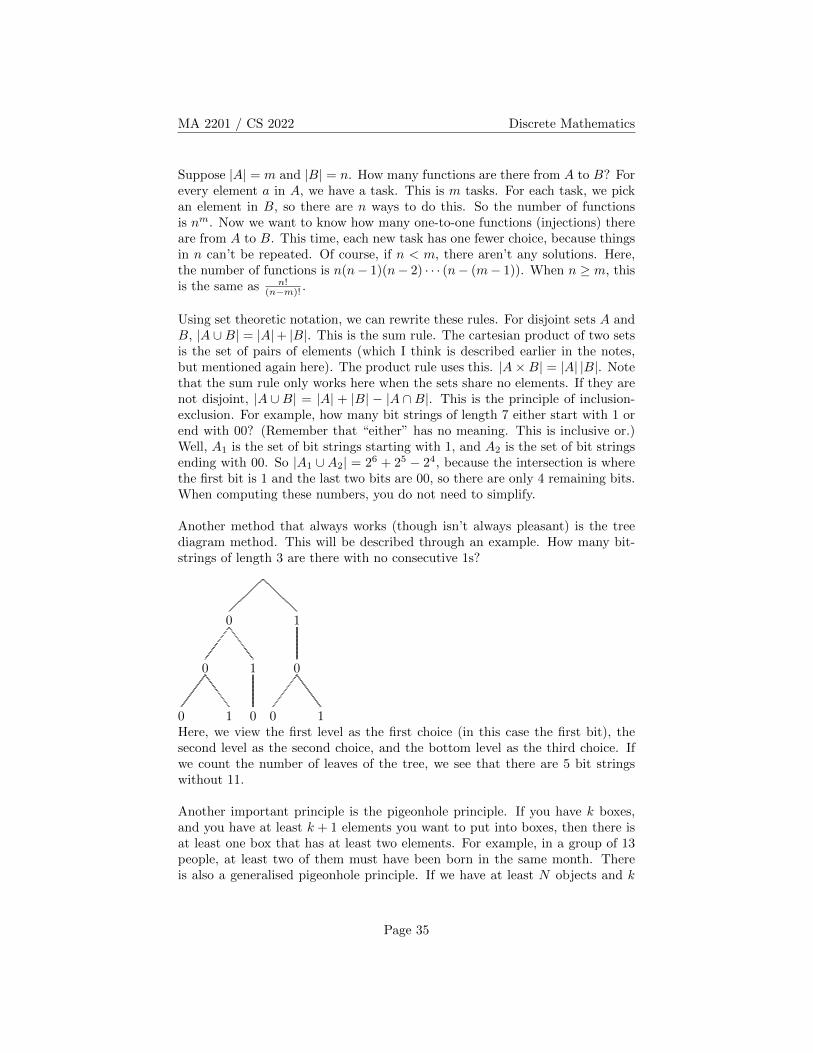
Another method that always works (though isn’t always pleasant) is the treediagram method. This will be described through an example. How many bit-strings of length 3 are there with no consecutive 1s?
1
0
10
0
1
0
0
10Here, we view the first level as the first choice (in this case the first bit), thesecond level as the second choice, and the bottom level as the third choice. Ifwe count the number of leaves of the tree, we see that there are 5 bit stringswithout 11.
Another important principle is the pigeonhole principle. If you have k boxes,and you have at least k + 1 elements you want to put into boxes, then there isat least one box that has at least two elements. For example, in a group of 13people, at least two of them must have been born in the same month. Thereis also a generalised pigeonhole principle. If we have at least N objects and k
Page 35
MA 2201 / CS 2022 Discrete Mathematics
boxes, then there will be a box with at least dNk e. We can prove this with asimple proof by contradiction. We first assume indirectly that every box canhave fewer than dNk e elements. In this case, the number of elements is at most
k(dNk e − 1
)Remember that dxe < x+1. So the number of elements is less than
k(Nk + 1− 1
)= N . But we have N elements, and N 6< N .
Suppose we have a group of 100 people, there must be at least x people whowere born in the same month. x = d 10012 e = 9. We might have more, but 9 isthe minimum.
11.1 A Spanning Review
The propositional operators we’ve looked at are negation (¬p), conjunction (p∧q), disjunction (p∨q), exclusive or (p⊕q), implication (p→ q), and biconditional(p↔ q). In order, these are true if: p is false; both are true; at least one is true;exactly one is true; p is false or q is true (or both); they are the same.
Quantified statements are of the form ∀xP (x) and ∃xP (x). In these, the predi-cate P (x) is a function. Every individual x gives a proposition. The first quan-tifier says that something is true for every x. The second says it is true for atleast one x. The negations are ¬∀xP (x) ≡ ∃x¬P (x) and ¬∃xP (x) ≡ ∀x¬P (x).
f : A→ B means that f is a function, it’s domain is A, and its codomain is B.For every element a ∈ A, f(a) is an element in B. The set of elements in B thatare images of things in A is called the range of f . One thing in A can’t have twoimages in B, and nothing in A can have zero images. Everything in A must havea single image in B. There are special functions that require certain things aboutthe elements of B. An injection, or a one-to-one function, requires every elementof B to have no more than one pre-image. Things in B are either the image ofa unique thing in A or they aren’t images. A surjection, or an onto function,requires every element of B to have at least one pre-image. Everything in thecodomain must be in the range. A bijection, or a one-to-one correspondance (oran invertible function), is both an injection and a surjection. Every element inB has exactly one pre-image. If f is an injection, then |A| ≤ |B| (where |A| isthe cardinality of A, or the number of elements in A). If f is a surjection, then|A| ≥ |B|. If f is a bijection, then |A| = |B|.
There are some rules of inference.Modus ponens: p→ q, p, ∴ q.Modus tollens: p→ q, ¬q, ∴ ¬p.Simplification: p ∧ q, ∴ p, q.Addition: p, ∴ p ∨ q.Hypothetical syllogism: p→ q, q → r, ∴ p→ r.Disjunctive syllogism: p ∨ q, ¬p, ∴ q.
Page 36
MA 2201 / CS 2022 Discrete Mathematics
Conjunction: p, q, ∴ p ∧ q.Resolution: p ∨ q, ¬p ∨ r, ∴ q ∨ r.Dilemma: p1 → q, p2 → q, p1 ∨ p2, ∴ q.
There are some common fallacies.Affirming the conclusion: p→ q, q, 6∴ p.Denying the hypothesis: p→ q, ¬p, 6∴ ¬q.Circular reasoning: p→ q, q → p, 6∴ p, q.
There are also quantified rules of inference.Universal instantiation: ∀xP (x), ∴ P (c).Universal generalization: For any c, P (c), ∴ ∀xP (x).Existential instantiation: ∃xP (x), ∴ P (c) for some c.Existential generalization: For some c, P (c), therefore ∀xP (x).Universal modus ponens: ∀x(P (x)→ Q(x), P (c), ∴ Q(c).Universal modus tollens: ∀x(P (x)→ Q(x), ¬Q(c), ∴ ¬P (c).
One of the harder proof techniques is an indirect proof. In this, we proveor disprove one thing which is equivalent to proving the given question. Forexample, proving p → q is equivalent to proving ¬q → ¬p. Also, if the goalis to prove p, a proof by contradiction assumes ¬p is true and then proves acontradiction (something that is always false). Often this contradiciton is of theform q ∧ ¬q.
Big Oh notation will not be on the exam. There was much rejoicing.
11.2 A Teeny Review
The sum rule is that, when either x or y happens, the number of things thatcan happen is the number of ways x can happen plus the number of ways ycan happen. The product rule says that, if x happens and then y happens,the total number of ways things can happen is the product of the number ofways x and y can happen. The principle of inclusion-exclusion is that |A ∪B| =|A| + |B| − |A ∩B|. The pigeonhole principle says that, if you have N objectsand k boxes, at least one box has at least dNk e objects. For example, in a groupof 100 people, at least 9 were born in the same month.
11.3 6 Party Theorem
This is a special case of Ramsey’s Theorem. In a group of 6 people, assume allpairs of people are either friends or enemies. We represent friends with solidlines and enemies with dotted lines. In this group, there must be 3 people who
Page 37
MA 2201 / CS 2022 Discrete Mathematics
are mutual friends (a solid triangle) or 3 people who are mutual enemies (adotted triangle).
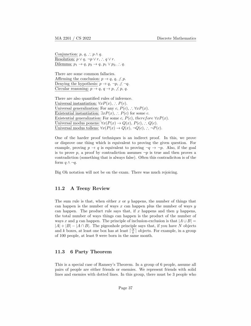
Pick one person x. There are 5 other people, so at least d 52e = 3 are eitherfriends or enemies of x. We will assume that 3 people are all friends with x (ifwe assumed incorrectly, just switch our labelling of friends and enemies in ourpictures).
x
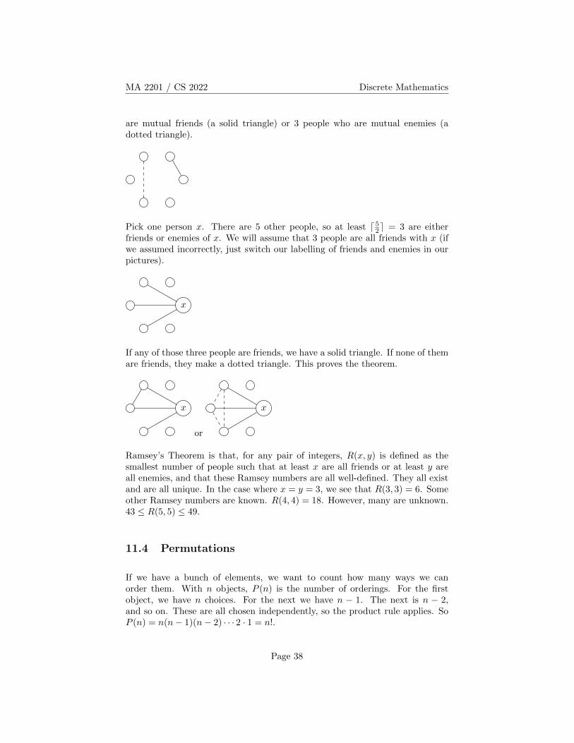
If any of those three people are friends, we have a solid triangle. If none of themare friends, they make a dotted triangle. This proves the theorem.
x
or
x
Ramsey’s Theorem is that, for any pair of integers, R(x, y) is defined as thesmallest number of people such that at least x are all friends or at least y areall enemies, and that these Ramsey numbers are all well-defined. They all existand are all unique. In the case where x = y = 3, we see that R(3, 3) = 6. Someother Ramsey numbers are known. R(4, 4) = 18. However, many are unknown.43 ≤ R(5, 5) ≤ 49.
11.4 Permutations
If we have a bunch of elements, we want to count how many ways we canorder them. With n objects, P (n) is the number of orderings. For the firstobject, we have n choices. For the next we have n − 1. The next is n − 2,and so on. These are all chosen independently, so the product rule applies. SoP (n) = n(n− 1)(n− 2) · · · 2 · 1 = n!.
Page 38
MA 2201 / CS 2022 Discrete Mathematics
We also talk about k-permutations, where we want to find the number of wayswe can order k of the elements. P (n, k) is this number. We again have n choicesfor the first and n− 1 for the second, but this time we only pick k things, so wego until n− k + 1 ways to pick the last thing. Again, the product rule applies,so we have P (n, k) = n!
(n−k)! ways to order them. For example, with 8 athletes,
how many ways can we give out gold, silver, and bronze? We can give gold to 8different people, then there are 7 people we can give silver to, and then 6 peopleto give bronze to, for 8 · 7 · 6 ways.
11.5 Combinations
If we don’t care about ordering, we talk about combinations rather than per-mutations. From the previous example, that would be if we didn’t care who gotwhich medal, and we only cared about the three people who got prizes. C(n, k)is this number, and it is often written as
(nk
), which is pronounced “n choose k”.
These are very important numbers, and are also called binomial coefficients. Tocompute this, we can consider permutations first. Then we divide by the num-
ber of ways to permute the people we picked. So C(n, k) = P (n,k)P (k,k) =
n!(n−k)!
k! =n!
k!(n−k)! .
11.6 A Tiny Review
Permutations are when we want to know how many ways there are to orderthings. k-permutations are when we want to order only k things from a set. Iforder doesn’t matter, and we only care about a subset, we talk about combi-nations. P (n, k) = n!
(n−k)! . C(n, k) =(nk
)= n!
k!(n−k)! . The middle thing there
is called “n choose k”. For example,(42
)= 4·3·2·1
2·1·2·1 = 6. Also, these are calledbinomial coefficients.
11.7 Properties of Binomial Coefficients
First, it is worth mentioning that binomial coefficients are symmetric.(nk
)=(
nn−k). We can either show this with an algebraic proof or with a combinatorial
Page 39
MA 2201 / CS 2022 Discrete Mathematics
proof. First we’ll use an algebraic proof.(n
n− k
)=
n!
(n− k)!(n− (n− k))!
=n!
(n− k)!(n− n+ k)!
=n!
(n− k)!(k)!
=n!
(k)!(n− k)!
=
(n
k
)The combinatorial proof is often rather simpler. In this case,
(nk
)means we
have a set of n elements, and we want to know how many ways we can pick kof them. That’s the same as asking how many ways we can leave out n − k ofthem. If we instead pick the ones we want to leave out, that’s
(n
n−k).
Next is Pascal’s indentity.(n+1k
)=(nk
)+(
nk−1). The combinatorial proof
is simpler here.(n+1k
)is the number of subsets of size k of n + 1 elements.
Consider one specific element x of the set. There are two cases: either x is inour subset or x is not in out subset, and these can’t both happen. In case 1,we pick k from the remaining n elements, and there are
(nk
)ways to do this. In
case 2, we have already picked 1 element, so we pick k − 1 elements from theremaining n. There are
(n
k−1)
ways to do this. So(n+1k
)=(nk
)+(
nk−1).
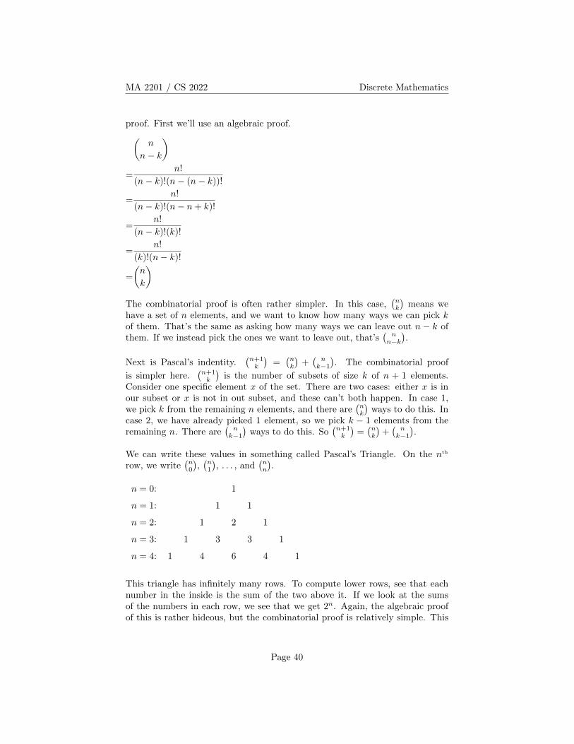
We can write these values in something called Pascal’s Triangle. On the nth
row, we write(n0
),(n1
), . . . , and
(nn
).
n = 0: 1
n = 1: 1 1
n = 2: 1 2 1
n = 3: 1 3 3 1
n = 4: 1 4 6 4 1
This triangle has infinitely many rows. To compute lower rows, see that eachnumber in the inside is the sum of the two above it. If we look at the sumsof the numbers in each row, we see that we get 2n. Again, the algebraic proofof this is rather hideous, but the combinatorial proof is relatively simple. This
Page 40
MA 2201 / CS 2022 Discrete Mathematics
identity isn∑
i=0
(n
i
)= 2n
Notice that(ni
)is the number of subsets of size i from a set of n elements. If we
sum over all values of i, that’s just the number of subsets of a set of n elements.From earlier in the class, recall that the cardinality of the power set of a setwith n elements is 2n.
The next identity is one about the squares of the binomial coefficients.
n∑i=0
(n
i
)2
=
n∑i=0
(n
i
)(n
n− i
)=
(2n
n
)Notice that the first and second things are true because of the symmetry weshowed earlier. Next let’s look at what the right side is counting. The numberof subsets of size n from a set of 2n elements. If we split the set into two parts,each of size n, then we can pick anything from 0 to n things from the first half.Call the number we pick from there i. Then we need to pick n − i from thesecond half. The number of ways to do this are
(ni
)(n
n−i). Because i can be
anything 0 to n, we sum over all values of i.
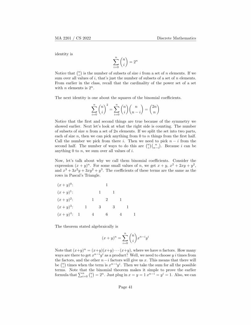
Now, let’s talk about why we call them binomial coefficients. Consider theexpression (x + y)n. For some small values of n, we get x + y, x2 + 2xy + y2,and x3 + 3x2y + 3xy2 + y3. The coefficients of these terms are the same as therows in Pascal’s Triangle.
(x+ y)0: 1
(x+ y)1: 1 1
(x+ y)2: 1 2 1
(x+ y)3: 1 3 3 1
(x+ y)4: 1 4 6 4 1
The theorem stated algebraically is
(x+ y)n =
n∑i=0
(n
i
)xn−iyi
Note that (x+y)n = (x+y)(x+y) · · · (x+y), where we have n factors. How manyways are there to get xn−iyi as a product? Well, we need to choose y i times fromthe factors, and the other n− i factors will give us x. This means that there willbe(ni
)times when the term is xn−iyi. Then we take the sum for all the possible
terms. Note that the binomial theorem makes it simple to prove the earlierformula that
∑ni=0
(ni
)= 2n. Just plug in x = y = 1 xn−i = yi = 1. Also, we can
Page 41
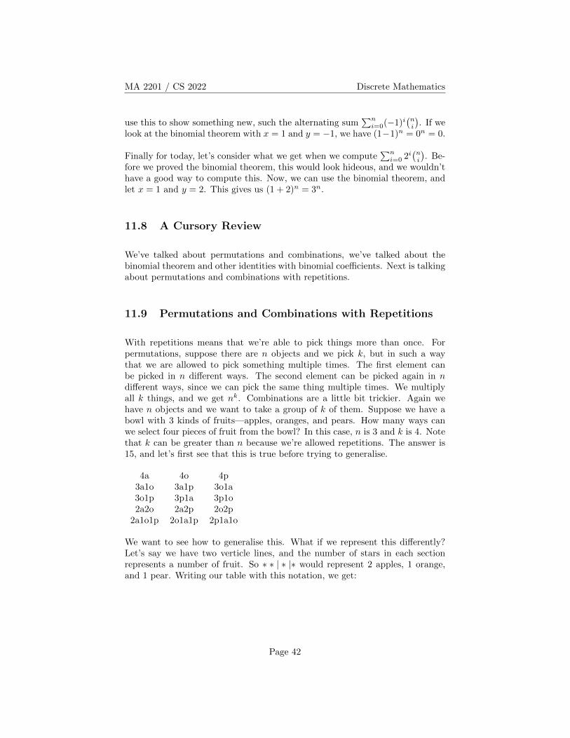
MA 2201 / CS 2022 Discrete Mathematics
use this to show something new, such the alternating sum∑n
i=0(−1)i(ni
). If we
look at the binomial theorem with x = 1 and y = −1, we have (1−1)n = 0n = 0.
Finally for today, let’s consider what we get when we compute∑n
i=0 2i(ni
). Be-
fore we proved the binomial theorem, this would look hideous, and we wouldn’thave a good way to compute this. Now, we can use the binomial theorem, andlet x = 1 and y = 2. This gives us (1 + 2)n = 3n.
11.8 A Cursory Review
We’ve talked about permutations and combinations, we’ve talked about thebinomial theorem and other identities with binomial coefficients. Next is talkingabout permutations and combinations with repetitions.
11.9 Permutations and Combinations with Repetitions
With repetitions means that we’re able to pick things more than once. Forpermutations, suppose there are n objects and we pick k, but in such a waythat we are allowed to pick something multiple times. The first element canbe picked in n different ways. The second element can be picked again in ndifferent ways, since we can pick the same thing multiple times. We multiplyall k things, and we get nk. Combinations are a little bit trickier. Again wehave n objects and we want to take a group of k of them. Suppose we have abowl with 3 kinds of fruits—apples, oranges, and pears. How many ways canwe select four pieces of fruit from the bowl? In this case, n is 3 and k is 4. Notethat k can be greater than n because we’re allowed repetitions. The answer is15, and let’s first see that this is true before trying to generalise.
4a 4o 4p3a1o 3a1p 3o1a3o1p 3p1a 3p1o2a2o 2a2p 2o2p
2a1o1p 2o1a1p 2p1a1o
We want to see how to generalise this. What if we represent this differently?Let’s say we have two verticle lines, and the number of stars in each sectionrepresents a number of fruit. So ∗ ∗ | ∗ |∗ would represent 2 apples, 1 orange,and 1 pear. Writing our table with this notation, we get:
Page 42
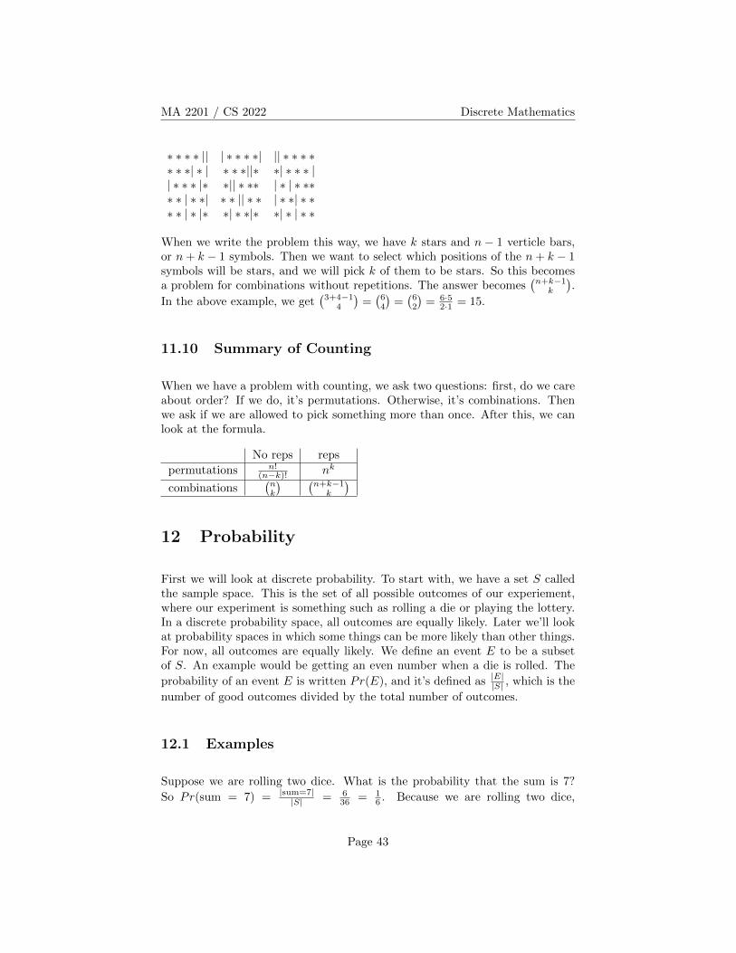
MA 2201 / CS 2022 Discrete Mathematics
∗ ∗ ∗ ∗ || | ∗ ∗ ∗ ∗| || ∗ ∗ ∗ ∗∗ ∗ ∗| ∗ | ∗ ∗ ∗||∗ ∗| ∗ ∗ ∗ || ∗ ∗ ∗ |∗ ∗|| ∗ ∗∗ | ∗ | ∗ ∗∗∗ ∗ | ∗ ∗| ∗ ∗ || ∗ ∗ | ∗ ∗| ∗ ∗∗ ∗ | ∗ |∗ ∗| ∗ ∗|∗ ∗| ∗ | ∗ ∗
When we write the problem this way, we have k stars and n − 1 verticle bars,or n+ k − 1 symbols. Then we want to select which positions of the n+ k − 1symbols will be stars, and we will pick k of them to be stars. So this becomesa problem for combinations without repetitions. The answer becomes
(n+k−1
k
).
In the above example, we get(3+4−1
4
)=(64
)=(62
)= 6·5
2·1 = 15.
11.10 Summary of Counting
When we have a problem with counting, we ask two questions: first, do we careabout order? If we do, it’s permutations. Otherwise, it’s combinations. Thenwe ask if we are allowed to pick something more than once. After this, we canlook at the formula.
No reps reps
permutations n!(n−k)! nk
combinations(nk
) (n+k−1
k
)
12 Probability
First we will look at discrete probability. To start with, we have a set S calledthe sample space. This is the set of all possible outcomes of our experiement,where our experiment is something such as rolling a die or playing the lottery.In a discrete probability space, all outcomes are equally likely. Later we’ll lookat probability spaces in which some things can be more likely than other things.For now, all outcomes are equally likely. We define an event E to be a subsetof S. An example would be getting an even number when a die is rolled. The
probability of an event E is written Pr(E), and it’s defined as |E||S| , which is the
number of good outcomes divided by the total number of outcomes.
12.1 Examples
Suppose we are rolling two dice. What is the probability that the sum is 7?
So Pr(sum = 7) = |sum=7||S| = 6
36 = 16 . Because we are rolling two dice,
Page 43
MA 2201 / CS 2022 Discrete Mathematics
there are six results for each of them, and we multiply them together to getatotal of 36 possible outcomes. Of these, the following six are in our event:(1, 6), (2, 5), (3, 4), (4, 3), (5, 2), (6, 1).
Suppose we’re playing a lottery in which we pick six numbers out of 40, and wewin when we get all six numbers correct. Notice that computing probabilitieshere is just two counting problems, and then dividing. In this case, the proba-
bility of winning is Pr(E) = |E||S| = 1
|S| . In this lottery, we only have one way to
win, because we only win if our chosen 6 were the correct chosen 6, and orderdoesn’t matter. There are 40 numbers, and |S| is the number of ways to pick 6.So Pr(E) = 1
(406 )≈ 1
4,000,000 .
Now suppose we’re playing cards with a standard deck of 52 playing cards. Thereare 13 ranks and 4 suits, and all suit-rank pairs have one card (that’s what adeck is). You are dealt 5 cards. What is Pr(Having a poker in your hand),where a poker is all 4 cards of some rank. In this case, |S| =
(525
). There are 52
cards, and you don’t care about the order in which you are dealt your 5. |E| inthis case is 13 · 48. There are 13 ways to select which poker you have, and thenyou have a fifth card which can be anything. Once you already have the poker,there are 48 other cards that can be your fifth. Because these are independentchoices, we multiply them. So Pr(E) = 13·48
(525 )
.
Suppose we have a bin containing numbered balls 1 through 50. We draw 5 ofthese balls. What is the probability that we draw 1, 2, 3, 4, and 5 in that order?This question has two parts. In the first part, we do not return the balls to thebin after drawing them. In the second part, we do put them back in. In both ofthese cases, |E| = 1, because there is only one thing that is what we want. Alsoin both cases, we are looking at permutations, because order matters. In part1, we do not have replacement, so |S| = P (50, 5). In part 2, we do, so |S| = 505.
12.2 A Little Review
In probability, S is the sample space, containing every possible outcome. E ⊆ Sis a subset of S, and it is called an event. The probability of an event in discrete
probability spaces is Pr(E) = |E||S| .
12.3 Operations on Events
The complement of an event E = S − E, and Pr(E) = frac|S| − |E||S| =1− Pr(E). The union of two events E1 and E2 has probability Pr(E1 ∪E2) =Pr(E1) + Pr(E2)− Pr(E1 ∩ E2).
Page 44
MA 2201 / CS 2022 Discrete Mathematics
Suppose we have a random bit string of length 10, and every bit has probability1/2 of being a 1. What it the probability of having at least one 1 as a bit? Using
the complement, this is 1− Pr(no 1) = 1−(12
)10.
Consider a random positive integer no greater than 100. What is the probabilitythat it is divisible by 2 or 5? E1 is divisible by 2, E2 is divisible by 5. Pr(E1 ∪E2) = Pr(E1) + Pr(E2)− Pr(E1 ∩ E2) = 50
100 + 20100 −
10100 = 60
100 = 35 .
12.4 General Probability Distributions
First we looked at discrete probability distributions, in which everything isequally likely. In general probability distributions, this is no longer the case. IfS = {x1, x2, . . . , xn}, then we require the following property for every value ofi: 0 ≤ Pr(xi) ≤ 1. Also, we require
∑ni=1 Pr(xi) = 1. Individual probabilities
must be within 0 and 1 (inclusive), and the sum has to be 1. We see thatthe probability of an event is Pr(E) =
∑xi∈E Pr(xi). Notice that if all the
probabilities are the same, we get the same equation as previously.
Consider a die in which rolling a 3 is twice as likely as rolling any other particularnumber. What is the probability of getting an odd number? To do this, we needto compute the probability of each outcome. Pr(1) = Pr(2) = Pr(4) = Pr(5) =Pr(6), and let’s call that number p. Pr(3) = 2p. Remember that this sum mustbe 1, so 5p+ 2p = 1, and p = 1
7 . Pr(odd number) = 1+2+17 = 4
7 .
12.5 Conditional Probability
If E and F are events, what is the probability of E, assuming we already knowthat F happened? We write this as Pr(E | F ). This is also known as condition-ing on F . This is sort of like restricting our sample space to F and looking at just
the portion of E that’s inside of F . We get the equation Pr(E | F ) = Pr(E∩F )Pr(F ) .
Consider a family with 2 children. E is the event that both children as boys.Pr(E) = 1
4 . F is the event that there is at least 1 boy. Pr(F ) = 34 . We’d like
to know Pr(E | F ). Our intuition can sometimes be misleading, so let’s look
at the formula. Notice that the intersection is the same as E, so Pr(E∩F )Pr(F ) =
Pr(E)Pr(F ) =
1/43/4 = 1
3 .
Suppose we have a random bit string of length 4. E is the event that we havetwo consecutive 0s. F is the event that we start with a 0. What is Pr(E | F )?We start with the formula, and the denominator is the easy part. Pr(F ) = 1
2 .The intersection is true when the second bit is zero or when both the last bits
Page 45
MA 2201 / CS 2022 Discrete Mathematics
are 0. The ways this can happen are 0000, 0001, 0010, 0011, 0100. There are 16bitstrings, so Pr(E ∩ F ) = 5
16 . So Pr(E | F ) = 58 .
12.6 Independence of Events
If E and F are events, we say that they are independent if Pr(E | F ) = Pr(E).
This gives us Pr(E∩F )Pr(F ) = Pr(E), or Pr(E ∩ F ) = Pr(E)Pr(F ).
In the example above with the children, notice that Pr(E ∩F ) 6= Pr(E)Pr(F ).Let’s change the problem so that they have 3 kids, E is the event that theyhave both a boy and a girl, and F is the event that they have at most oneboy. To see if these are independent or not, let’s compute the probabilities ofeverything. Pr(E) is a bit tricky to compute, but Pr(E) is a lot easier. Out of8 possibilities, there are 2 ways to have all boys or all girls. So Pr(E) = 3
4 . Tocompute Pr(F ), we can list the ways it can happen: GGG, BGG, GBG, andGGB, so Pr(F ) = 1
2 . If we compute Pr(E ∩ F ), we can look at the ways Fcan happen and see how many of them satisfy E. There are 3 ways this canhappen, so Pr(E ∩ F ) = 3
8 = 1234 , so the events are independent.
12.7 Bernouli Trials and the Binomial Distribution
In a Bernouli trial, there are two outcomes: success and failure. We denotePr(success) = p and Pr(failure) = 1 − p = q. If we have a sequence of nindependent Bernouli trials, we would like to know the probability of havingexactly k successes. This probability distribution is a binomial distribution.We give this special notation: b(k, n, p) = Pr(exactly k successes). Using whatwe’ve seen already, we can show that b(k, n, p) =
(nk
)pk(1 − p)n−k. This first
picks which positions will be successes, then computes the chance of havingsuccess at those positions, and then the chance of failures are the other positions.Seeing the binomial coefficients will be a clue as to why we call this a binomialdistribution.
Suppose we toss a biased coin 7 times, and this coin comes up heads 23 of the
time and tails 13 of the time. The probability of getting exactly 3 heads is
b(3, 7, 23 ) =(73
) (23
)3 ( 13
)4. Notice that, if we take the sum over all k of b(k, n, p),
we get 1, and this comes from the binomial theorem, when x = p and y = 1−p.
Page 46
MA 2201 / CS 2022 Discrete Mathematics
12.8 An Abbreviated Review
The binomial distribution is an important distribution. From a sequence of nindependent Bernouli trials, it counts the number of successes, when the proba-bility of a given trial being a success is p. P (exactly k successes) = b(k, n, p) =(nk
)pk(1− p)n−k.
12.9 Random Variables
Random variables are pooly named. They aren’t random and they aren’t vari-ables. They are a function from a sample space S to the real numbers R. Theyare almost always written as capital letters, such as X : S → R.
For example, if we toss a coin 3 times, X can be the number of heads. In thatcase, X(HHT ) = 2, because HHT is an outcome in the sample space, and thenumber of heads is 2. The function doesn’t need to be an injection (one-to-one),as can be seen with X(HTH) is also 2. Likewise, if we roll two dice, Y can bethe sum of the faces. In this case, Y
((1, 3)
)= 4.
The expected value of a random variable is denoted E(X), and it is a weightedaverage of all the outcomes. E(X) =
∑s∈S Pr(s)X(s). It can sometimes be
easier to group things by the value of X, in which case we write E(X) =∑r∈X(S) Pr(X = r)r. Here, notice that X = r is an event. Also, that sum
notation with r ∈ X(S) is a bit different from what we’re used to.∑5
k=1 meansthat k has the values 1, 2, 3, 4, and 5. In
∑r∈X(S), r has all the values that
appear as images of X.
Using our coin-flipping example above, let’s compute the expected value of X.Each outcome has probability 1
8 , so we get E(X) = 18
(X(TTT ) + X(HTT ) +
X(THT )+X(TTH)+X(HHT )+X(HTH)+X(THH)+X(HHH))
= 18 (0+
1+1+1+2+2+2+3) = 128 = 3
2 . This makes sense, as flipping a coin once hasan average value of half a heads. If we use the other way of computing expectedvalues, we need to compute Pr(X = k) for k = 0, 1, 2, 3. Using the binomialcoefficients, we see that the number of ways to have those values of k are 1, 3,3, and 1, respectively. The total number of outcomes is 8, so the probabilitiesare those coefficients divided by 8. So E(X) = 1
80 + 381 + 3
82 + 183 = 3+6+3
8 = 32 .
If we look at rolling one die, E(Y ) = 16 (1 + 2 + 3 + 4 + 5 + 6) = 21
6 = 72 .
With a binomial distribution, let X be the number of successes. We will showthat E(X) = pn. First we’ll use the definition of expected values. E(X) =∑n
k=0 k · Pr(X = k) =∑n
k=0 k(nk
)pk(1 − p)n−k. This is the r ∈ X(S) sum-
mation, and we know that the possible values are the integers 0 to n. k is thevalue, and we take the weighted average by weighting it against Pr(X = k).
Page 47
MA 2201 / CS 2022 Discrete Mathematics
Looking at the terms we have, k(nk
)= k n!
k!(n−k)! = n (n−1)!(k−1)!(n−k)! = n
(n−1k−1).
Putting this back into our equation gives E(X) =∑n
k=0 n(n−1k−1)pk(1− p)n−k =
np∑n
k=0
(n−1k=1
)pk−1(1− p)n−k, because we can factor out np, since that doesn’t
depend on k. Using the binomial theorem, E(X) = np∑n
k=0
(n−1k=1
)pk−1(1 −
p)n−k = np(p+ (1− p)
)n−1= np(1) = np.
12.10 Linearity of Expectation
Something very important to us is that the expected value of a sum of randomvariables is the sum of the expected values of those random variables. That is,E(X1 +X2 + · · ·+Xn) = E(X1) + E(X2) + · · ·+ E(Xn). Similarly, E(aX) =aE(X). We can see this from our defintion: E(X1+X2) =
∑s∈S Pr(s)
(X1(s)+
X2(s))
=∑
s∈S Pr(s)X1(s) +∑
s∈S Pr(s)X2(s) +E(X1) +E(X2). Suppose weroll 2 dice, X1 is the result of the first die, X2 is the result of the second die,and X is the sum of these. Without the linearity of expectation, we’d needto consider a sample space with 36 outcomes. Instead, we see that E(X) =E(X1 +X2) = E(X1) + E(X2) = 7
2 + 72 = 7.
Going back to the binomial distribution, we can find the expected value muchmore easily now. X is the number of successes over the n trials. Let Xi be thenumber of successes in the ith Bernouli trial. So E(X) =
∑ni=0E(X1). For each
Xi, E(Xi) = 1 · Pr(Xi = 1) + 0 · Pr(Xi = 0) = 1 · p + 0 · (1 − p) = p. So thesum of n of these is np.
Often, when we have a complicated random variable, we can do what we didabove, and decompose it into the sum of several indicator random variables.Once we’ve done that, we can use the linearity of expectation to find the ex-pected value of our complicated random variable.
12.11 Hat-Check Problem
n people check in their hats, and they all get hats at the end of the event.However, the people working at the hat check are horrible at their job, and theygive back the hats at random. Let X count the number of people who get thecorrect hat. We’d like to compute E(X). Somewhat surprisingly, E(X) = 1. Wewill see this by decomposing our random variable. Let the n indicator randomvariables be
Xi =
{1 if the ith person gets back the right hat0 otherwise
Page 48
MA 2201 / CS 2022 Discrete Mathematics
Each indicator random variable has E(Xi) = 1n , because there is one correct
hat and n possible hats. So For E(X), we take the sum of all n E(Xi)s, and weget E(X) = 1.
12.12 A Compressed Review
Recall that for a random variable X, the expected value of X is E(X) =∑r∈X(S) r · Pr(X = r). Also, the expected value of the sum of two random
variables is E(X1 +X2) = E(X1) + E(X2).
12.13 Independent Random Variables
Two random variables are independent if Pr(X1 = r1 and X2 = r2) = Pr(X1 =r1) · Pr(X2 = r2). For example, consider rolling two dice. Let X1 be the resultof the first die and let X2 be the result of the second die. For every pair (i, j),where 1 ≤ i ≤ 6 and 1 ≤ j ≤ 6, we get that 1
36 = Pr(X1 = i ∧ X2 = j) =Pr(X1 = i)Pr(X2 = j) = 1
616 , so these two variables are independent. However,
now consider X1 still as the result of the first die, but now X3 as the sum of thetwo dice. 1
36Pr(X1 = 1 ∧X3 = 2) 6= Pr(X1 = 1)Pr(X3 = 2) = 16
136 , so these
two variables are dependent.
If two variables are independent, then we can do more than just add their ex-pected values. For independent variables, we also have the equation E(X1X2) =E(X1)E(X2). Showing this isn’t too difficult.
E(X1X2) =∑
r∈X1X2(S)
rPr(X1X2 = r)
=∑
r1∈X1(S)r2∈X2(S)
r1r2Pr(X1 = r1 ∧W2 = r2)
=∑
r1∈X1(S)r2∈X2(S)
r1r2Pr(X1 = r1)Pr(X2 = r2)
=
∑r1∈X1(s)
r1Pr(X1 = r1)
∑r2∈X2(s)
r2Pr(X2 = r2)
= E(X1)E(X2)
Page 49
MA 2201 / CS 2022 Discrete Mathematics
12.14 Variance
Expected value can be thought of as the center of the possible values. Varianceis a way of measuring how far things are from the center on average. The
variance of a random variable is given by V (X) = E(X2) =(E(X)
)2. We also
define the standard deviation as σ(X) =√V (X), but it’s not very important
for us.
Suppose we have a Bernoulli Trial with probability p of success. The expectedvalue E(X) = p, because X can be 1 with probability p, 0 with probability1−p, and 1 ·p+0 · (1−p) = p. E(X2) is again p, because 12 ·p+02 · (1−p) = p.So V (X) = p− p2 = p(1− p) = pq.
For independent random variables X and Y , we have linearity of variance.
V (X + Y ) = E((X + Y )2
)−(E(X) + E(Y )
)2= E
(X2 + 2XY + Y 2
)−((E(X)
)2+ 2E(X)E(Y ) +
(E(Y )
)2)= E(X2) + 2E(XY ) + E(Y 2)−
(E(X)
)2 − 2E(X)E(Y )−(E(Y )
)2= E(X2)−
(E(X)
)2+ E(Y 2)−
(E(Y )
)2= V (X) + V (Y )
Consider rolling two dice. Let X1 be the result of the first die and X2 the resultof the second. We want to compute the variance of the sum. V (X1 + X2) =V (X1) + V (X2) = 35
12 + 3512 = 35
6 .
For the variance of the binomial distribution, it’s n independent Bernoulli trials.Each trial has variance pq, so the variance of the distribution is npq.
13 Relations
Recall the cartesian product of two sets is A × B = {(a, b) | a ∈ A, b ∈ B}.A relation R is a subset of the cartesian product of two sets. For example, letA = {0, 1, 2}, B = {a, b}, and R = {(0, a), (0, b), (2, a)}.
We can represent relations with directed graphs. Each element of A∪B becomesa vertex in the graph (we’ll look more formally at graphs later), and the pair(x, y) becomes an edge from x to y. The above relation becomes the graph:
Page 50
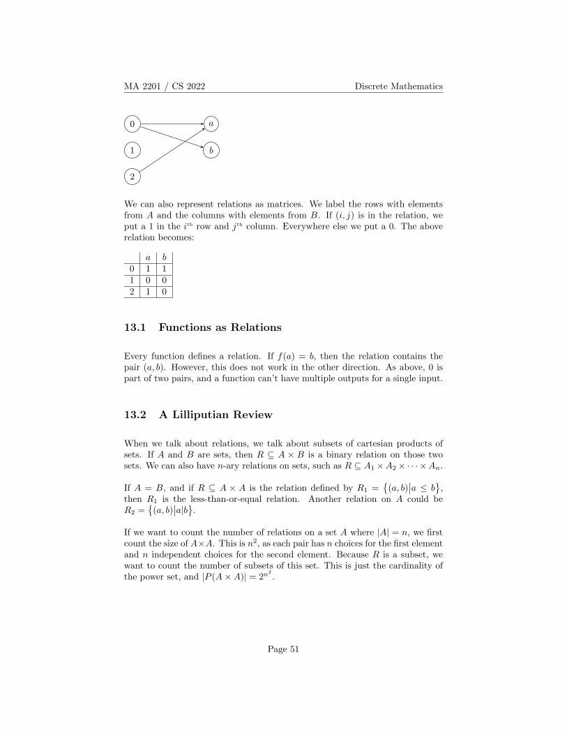
MA 2201 / CS 2022 Discrete Mathematics
0
1
2
a
b
We can also represent relations as matrices. We label the rows with elementsfrom A and the columns with elements from B. If (i, j) is in the relation, weput a 1 in the ith row and jth column. Everywhere else we put a 0. The aboverelation becomes:
a b0 1 11 0 02 1 0
13.1 Functions as Relations
Every function defines a relation. If f(a) = b, then the relation contains thepair (a, b). However, this does not work in the other direction. As above, 0 ispart of two pairs, and a function can’t have multiple outputs for a single input.
13.2 A Lilliputian Review
When we talk about relations, we talk about subsets of cartesian products ofsets. If A and B are sets, then R ⊆ A × B is a binary relation on those twosets. We can also have n-ary relations on sets, such as R ⊆ A1×A2× · · · ×An.
If A = B, and if R ⊆ A × A is the relation defined by R1 ={
(a, b)∣∣a ≤ b
},
then R1 is the less-than-or-equal relation. Another relation on A could beR2 =
{(a, b)
∣∣a|b}.
If we want to count the number of relations on a set A where |A| = n, we firstcount the size of A×A. This is n2, as each pair has n choices for the first elementand n independent choices for the second element. Because R is a subset, wewant to count the number of subsets of this set. This is just the cardinality ofthe power set, and |P (A×A)| = 2n
2
.
Page 51
MA 2201 / CS 2022 Discrete Mathematics
13.3 Properties of Relations
A relation R is reflexive if, ∀a ∈ A, (a, a) ∈ R. For example, the less-than-or-equal relation is reflexive, but the less-than relation is not.
A relation R is irreflexive if the above is false for each a. That is, if ∀a ∈ A,(a, a) 6∈ R. Note that a relation doesn’t need to be either reflexive nor irreflexive.
A relation R is symmetric if((a, b) ∈ R
)→((b, a) ∈ R
). Whenever (a, b) is in
the relation, (b, a) is also included. Neither of the relations we’ve written downare symmetric, so let’s look at R3 =
{(a, b)
∣∣a ≡ b mod 3}
. That is, pairs for
which 3 | b− a. Another example is R4 ={
(a, b)∣∣a+ b ≤ 10
}.
Similarly, we can have antisymmetric relations. In these, if we have (a, b), (b, a) ∈R, then it is required that a = b. R1 is an example of this.
Lastly, we talk about transitive relations. If (a, b) and (b, c) are in the relation,then (a, c) is in the relation. Two good examples are R1 and R2. R4 is nottransitive, and we observe this when we look at (9, 1) and (1, 9). The pair (9, 9)is not in the relation.
13.4 Operations on Relations
Since relations are just sets, we can use all of our set operations on them. Wecan look at R1∪R2, R1∩R2, R1 \R2, and a new one, R1⊕R2. These are union,intersection, difference, and symmetric difference. R1⊕R2 = (R1\R2)∪(R2\R1).We use ⊕ for this because it’s sort of like exclusive or. We include somethingin R1 ⊕R2 if it is in R1 or R2 but not if it’s in both.
The composition of two relations takes two relations R ⊆ A×B and S ⊆ B×C.S ◦ R =
{(a, c)
∣∣∃b ∈ B, (a, b) ∈ R, (b, c) ∈ S}. Note that R comes second, buta comes first. We can use this to define powers of a relation. R2 = R ◦ R, andRn+1 = Rn ◦R = R ◦Rn.
Consider the relation R ={
(1, 1), (2, 1), (3, 2), (4, 3)}
. When we compute R2,
we get the set{
(1, 1), (2, 1), (3, 1), (4, 2)}
. Next we compute the cube, and we
get the set{
(1, 1), (2, 1), (3, 1), (4, 1)}
. If we try to keep going, we see that therelation will no longer change when we take higher powers. Note that this is aproperty we’ve already defined. If Rn ⊆ R ∀n ≥ 1, that is the same as sayingthat R is transitive. Proving this requires showing both directions.
If Rn ⊆ R for all n, show that R is transitive. In fact, we can look at just thecase when n = 2, and that’s sufficient. Suppose our relation has pairs (a, b)
Page 52
MA 2201 / CS 2022 Discrete Mathematics
and (b, c). Because R2 ⊆ R, we can get rid of the middle element and havesomething in R2, so it must also be in R. So (a, c) is in R. This is what itmeans to be transitive, so R is transitive.
If R is transitive, show that Rn ⊆ R for all n. We will prove this with induction.Note that our basis case, when n = 1, is always true, even if R isn’t transitive.R ⊆ R. Now for the inductive step, we will assume for some n that Rn ⊆ R,and we will show that Rn+1 ⊆ R. Take a pair (a, c) ∈ Rn+1 = R ◦ Rn. Thereexists a b such that (a, b) ∈ Rn and (b, c) ∈ R. Because Rn ⊆ R, (a, b) ∈ R.Because R is transitive, (a, c) must also be in R, and Rn+1 is a subset of R. �
13.5 Matrices Representing Relations
If R is a relation on A × A, then we can make a matrix with 0s and 1s with|A| rows and columns. Put a 1 in the entry Mi,j if (i, j) ∈ R, and put 0severywhere else. If R is reflexive, then the diagonal must be entirely 1s. If R isirreflexive, then the diagonal must be entirely 0s. Note that this makes it easyto see that some relations are neither reflexive nor irreflexive, as we could havea diagonal consisting of both 1s and 0s. If R is symmetric, then MT = M . MT
is the mirror image across the main diagonal (from top left to bottom right).If this mirror image is equal to the original matrix, then the matrix is calledsymmetric, and the corresponding relation is symmetric. We call this operationT the transpose.
If we have two relations R1 and R2, we want to know what the matrix oftheir union looks like. MR1∪R2
= MR1∨MR2
. This is the bitwise OR of thematrices. Similarly, MR1∩R2 = MR1 ∧MR2 , where we use the bitwise AND forthe intersection. What about the matrix for MS◦R? We’ll look more at thisnext time, but the answer is MR �MS .
13.6 A Skimpy Review
We talked about a few relations. Reflexive relations have every pair (a, a),irreflexive relations leave out every pair (a, a), symmetric relations always have(a, b) if they have (b, a), antisymmetric relations always don’t have (a, b) if theyhave (b, a), and transitive relations always have (a, c) if they have both (a, b)and (b, c).
If R is a transitive relation, then Rn ⊆ R for every n ≥ 1. If we have matricesof relations, MR1∪R2
= MR1∨MR2
and MR1∩R2= MR1
∧MR2. The matrix of
the composition of relations MS◦R is related to matrix multiplication.
Page 53
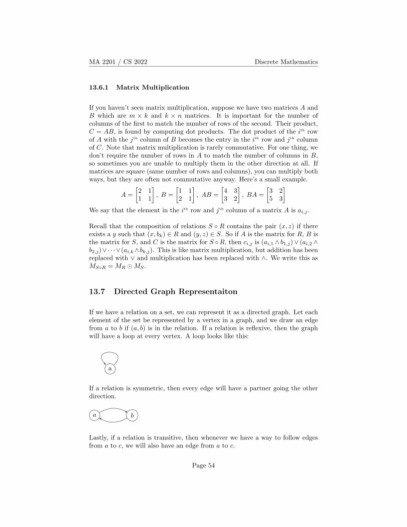
MA 2201 / CS 2022 Discrete Mathematics
13.6.1 Matrix Multiplication
If you haven’t seen matrix multiplication, suppose we have two matrices A andB which are m × k and k × n matrices. It is important for the number ofcolumns of the first to match the number of rows of the second. Their product,C = AB, is found by computing dot products. The dot product of the ith rowof A with the jth column of B becomes the entry in the ith row and jth columnof C. Note that matrix multiplication is rarely commutative. For one thing, wedon’t require the number of rows in A to match the number of columns in B,so sometimes you are unable to multiply them in the other direction at all. Ifmatrices are square (same number of rows and columns), you can multiply bothways, but they are often not commutative anyway. Here’s a small example.
A =
[2 11 1
], B =
[1 12 1
], AB =
[4 33 2
], BA =
[3 25 3
]We say that the element in the ith row and jth column of a matrix A is ai,j .
Recall that the composition of relations S ◦ R contains the pair (x, z) if thereexists a y such that (x, bk) ∈ R and (y, z) ∈ S. So if A is the matrix for R, B isthe matrix for S, and C is the matrix for S ◦R, then ci,j is (ai,1 ∧ b1,j)∨ (ai,2 ∧b2,j)∨· · ·∨(ai,k∧bk,j). This is like matrix multiplication, but addition has beenreplaced with ∨ and multiplication has been replaced with ∧. We write this asMS◦R = MR �MS .
13.7 Directed Graph Representaiton
If we have a relation on a set, we can represent it as a directed graph. Let eachelement of the set be represented by a vertex in a graph, and we draw an edgefrom a to b if (a, b) is in the relation. If a relation is reflexive, then the graphwill have a loop at every vertex. A loop looks like this:
a
If a relation is symmetric, then every edge will have a partner going the otherdirection.
a b
Lastly, if a relation is transitive, then whenever we have a way to follow edgesfrom a to c, we will also have an edge from a to c.
Page 54
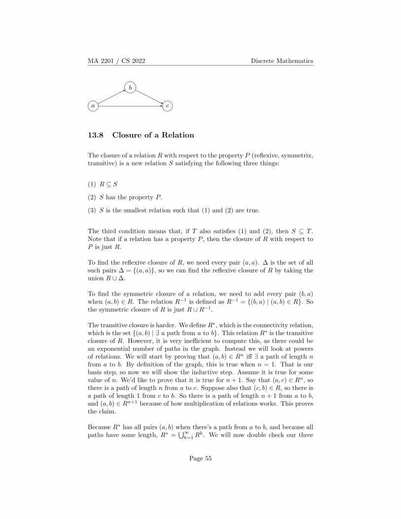
MA 2201 / CS 2022 Discrete Mathematics
a
b
c
13.8 Closure of a Relation
The closure of a relation R with respect to the property P (reflexive, symmetrix,transitive) is a new relation S satisfying the following three things:
(1) R ⊆ S
(2) S has the property P .
(3) S is the smallest relation such that (1) and (2) are true.
The third condition means that, if T also satisfies (1) and (2), then S ⊆ T .Note that if a relation has a property P , then the closure of R with respect toP is just R.
To find the reflexive closure of R, we need every pair (a, a). ∆ is the set of allsuch pairs ∆ = {(a, a)}, so we can find the reflexive closure of R by taking theunion R ∪∆.
To find the symmetric closure of a relation, we need to add every pair (b, a)when (a, b) ∈ R. The relation R−1 is defined as R−1 = {(b, a) | (a, b) ∈ R}. Sothe symmetric closure of R is just R ∪R−1.
The transitive closure is harder. We defineR∗, which is the connectivity relation,which is the set {(a, b) | ∃ a path from a to b}. This relation R∗ is the transitiveclosure of R. However, it is very inefficient to compute this, as there could bean exponential number of paths in the graph. Instead we will look at powersof relations. We will start by proving that (a, b) ∈ Rn iff ∃ a path of length nfrom a to b. By definition of the graph, this is true when n = 1. That is ourbasis step, so now we will show the inductive step. Assume it is true for somevalue of n. We’d like to prove that it is true for n+ 1. Say that (a, c) ∈ Rn, sothere is a path of length n from a to c. Suppose also that (c, b) ∈ R, so there isa path of length 1 from c to b. So there is a path of length n + 1 from a to b,and (a, b) ∈ Rn+1 because of how multiplication of relations works. This provesthe claim.
Because R∗ has all pairs (a, b) when there’s a path from a to b, and because allpaths have some length, R∗ =
⋃∞k=1R
k. We will now double check our three
Page 55
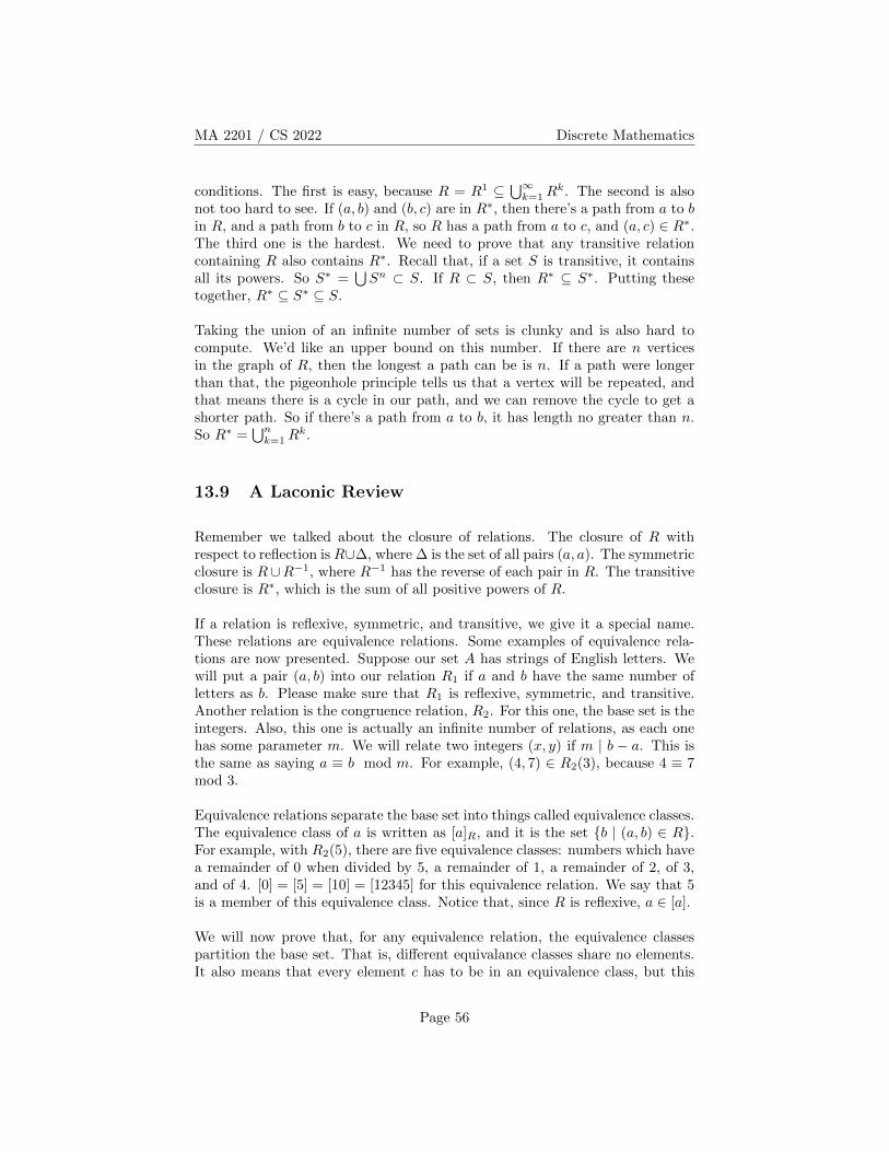
MA 2201 / CS 2022 Discrete Mathematics
conditions. The first is easy, because R = R1 ⊆⋃∞
k=1Rk. The second is also
not too hard to see. If (a, b) and (b, c) are in R∗, then there’s a path from a to bin R, and a path from b to c in R, so R has a path from a to c, and (a, c) ∈ R∗.The third one is the hardest. We need to prove that any transitive relationcontaining R also contains R∗. Recall that, if a set S is transitive, it containsall its powers. So S∗ =
⋃Sn ⊂ S. If R ⊂ S, then R∗ ⊆ S∗. Putting these
together, R∗ ⊆ S∗ ⊆ S.
Taking the union of an infinite number of sets is clunky and is also hard tocompute. We’d like an upper bound on this number. If there are n verticesin the graph of R, then the longest a path can be is n. If a path were longerthan that, the pigeonhole principle tells us that a vertex will be repeated, andthat means there is a cycle in our path, and we can remove the cycle to get ashorter path. So if there’s a path from a to b, it has length no greater than n.So R∗ =
⋃nk=1R
k.
13.9 A Laconic Review
Remember we talked about the closure of relations. The closure of R withrespect to reflection is R∪∆, where ∆ is the set of all pairs (a, a). The symmetricclosure is R∪R−1, where R−1 has the reverse of each pair in R. The transitiveclosure is R∗, which is the sum of all positive powers of R.
If a relation is reflexive, symmetric, and transitive, we give it a special name.These relations are equivalence relations. Some examples of equivalence rela-tions are now presented. Suppose our set A has strings of English letters. Wewill put a pair (a, b) into our relation R1 if a and b have the same number ofletters as b. Please make sure that R1 is reflexive, symmetric, and transitive.Another relation is the congruence relation, R2. For this one, the base set is theintegers. Also, this one is actually an infinite number of relations, as each onehas some parameter m. We will relate two integers (x, y) if m | b − a. This isthe same as saying a ≡ b mod m. For example, (4, 7) ∈ R2(3), because 4 ≡ 7mod 3.
Equivalence relations separate the base set into things called equivalence classes.The equivalence class of a is written as [a]R, and it is the set {b | (a, b) ∈ R}.For example, with R2(5), there are five equivalence classes: numbers which havea remainder of 0 when divided by 5, a remainder of 1, a remainder of 2, of 3,and of 4. [0] = [5] = [10] = [12345] for this equivalence relation. We say that 5is a member of this equivalence class. Notice that, since R is reflexive, a ∈ [a].
We will now prove that, for any equivalence relation, the equivalence classespartition the base set. That is, different equivalance classes share no elements.It also means that every element c has to be in an equivalence class, but this
Page 56
MA 2201 / CS 2022 Discrete Mathematics
is easy to show, because c ∈ [c]. First, we will show that the following threethings are all the same. (a, b) ∈ R, [a] = [b], and [a] ∩ [b] 6= ∅. The last two willshow that, if the intersection of two equivalence classes is not empty, then theyare the same equivalence class. We will show that the first statement impliesthe second, the second implies the third, and the third implies the first. Thiswill prove that the three are equivalent.
Assume (a, b) ∈ R. We want to show that [a] = [b]. To show that the twosets are the same, we need to show that each set is a subset of the other set.Let’s pick an arbitrary element c ∈ [a]. Because of the definition of [a], weknow that (a, c) ∈ R. Because [a] = [b], we know that (a, b) ∈ R. Becausethe relation is symmetric, (b, a) ∈ R. Because R is transitive, (b, c) ∈ R, whichmeans that c ∈ [b]. To show the other direction, copy and paste the abovetext, starting from “Let’s pick”, replacing a and b each time they appear. So((a, b) ∈ R
)⇒([a] = [b]
).
Now we will show that [a] = [b] implies [a] ∩ [b] 6= ∅. We know that a ∈ [a].Because the sets are equal, we know that a ∈ [b]. This means that a ∈
([a]∩ [b]
),
so the intersection is not the empty set. This one was easier.
Lastly, we will show that [a]∩[b] 6= ∅ implies (a, b) ∈ R. Because the intersectionis not empty, there is some element c ∈
([a]∩ [b]
). So (a, c) ∈ R, and (b, c) ∈ R.
Using symmetry, (c, b) ∈ R. Now using transitivity, (a, b) ∈ R. Because we havea circle of implications, the three statements are all equivalent.
13.10 Partial Orderings
A relation R is a partial ordering if it is reflexive, antisymmetric, and transitive.A set A with a partial ordering R is called a partially ordered set or a poset.For example, consider the relation R1 defined on R by (a, b) ∈ R1 iff a ≤ b.As another example, consider the relation R2 defined on Z by (a, b) ∈ R2 iffa | b. For our last example, consider the relation R3 defined on P ({1, 2, 3, 4}),the powerset of {1, 2, 3, 4}, given by (a, b) ∈ R3 iff a ⊆ b.
Why do we call them partial orderings? Well, we call a pair (a, b) comparableif either (a, b) or (b, a) is in the relation. For example, under R2, 3 and 5 arenot comparable, but 12 and 2 are. If every pair is comparable, we say therelation is a total ordering. Of the above three examples, only R1 is a totalordering. That’s it for this section, and next time we’ll start graph theory,which is Sarkozy’s favourite topic in this course.
Page 57
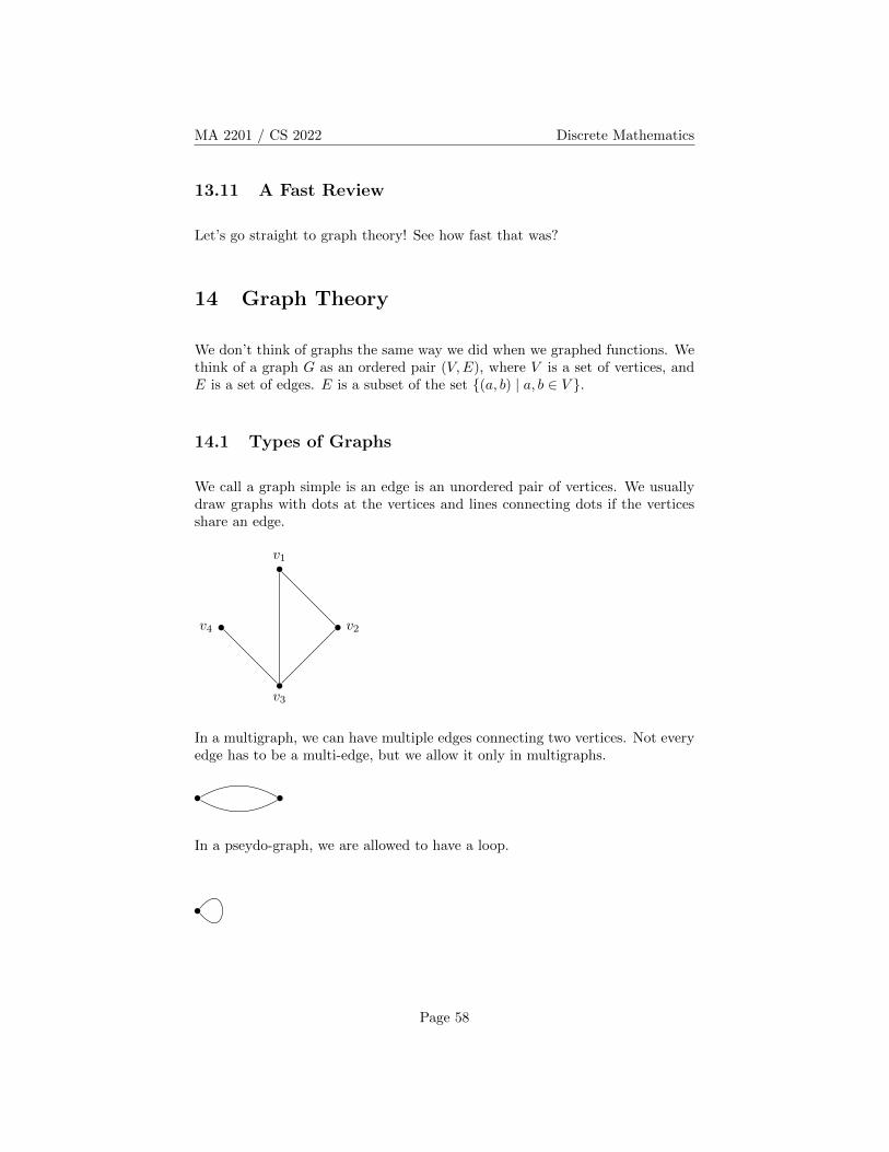
MA 2201 / CS 2022 Discrete Mathematics
13.11 A Fast Review
Let’s go straight to graph theory! See how fast that was?
14 Graph Theory
We don’t think of graphs the same way we did when we graphed functions. Wethink of a graph G as an ordered pair (V,E), where V is a set of vertices, andE is a set of edges. E is a subset of the set {(a, b) | a, b ∈ V }.
14.1 Types of Graphs
We call a graph simple is an edge is an unordered pair of vertices. We usuallydraw graphs with dots at the vertices and lines connecting dots if the verticesshare an edge.
v1
v2
v3
v4
In a multigraph, we can have multiple edges connecting two vertices. Not everyedge has to be a multi-edge, but we allow it only in multigraphs.
In a pseydo-graph, we are allowed to have a loop.
Page 58
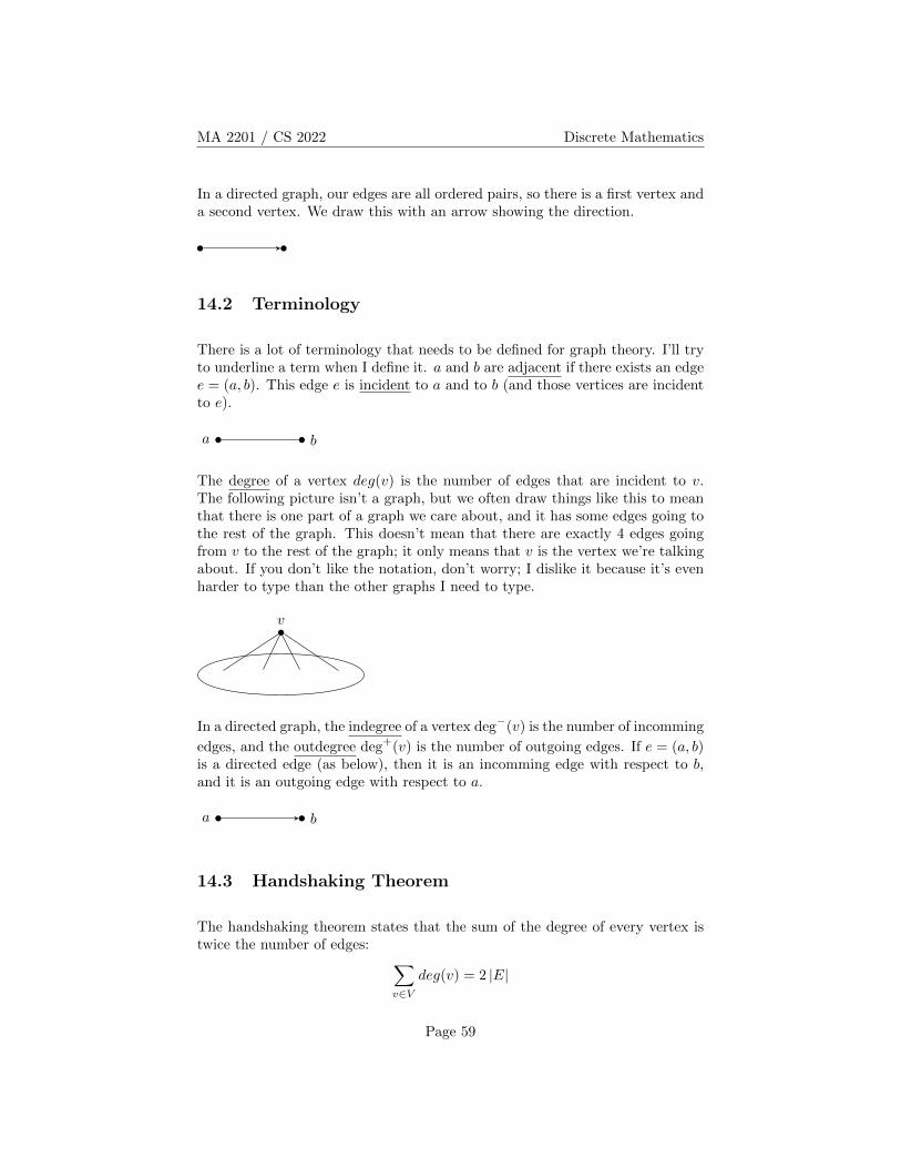
MA 2201 / CS 2022 Discrete Mathematics
In a directed graph, our edges are all ordered pairs, so there is a first vertex anda second vertex. We draw this with an arrow showing the direction.
14.2 Terminology
There is a lot of terminology that needs to be defined for graph theory. I’ll tryto underline a term when I define it. a and b are adjacent if there exists an edgee = (a, b). This edge e is incident to a and to b (and those vertices are incidentto e).
a b
The degree of a vertex deg(v) is the number of edges that are incident to v.The following picture isn’t a graph, but we often draw things like this to meanthat there is one part of a graph we care about, and it has some edges going tothe rest of the graph. This doesn’t mean that there are exactly 4 edges goingfrom v to the rest of the graph; it only means that v is the vertex we’re talkingabout. If you don’t like the notation, don’t worry; I dislike it because it’s evenharder to type than the other graphs I need to type.
v
In a directed graph, the indegree of a vertex deg−(v) is the number of incomming
edges, and the outdegree deg+(v) is the number of outgoing edges. If e = (a, b)is a directed edge (as below), then it is an incomming edge with respect to b,and it is an outgoing edge with respect to a.
a b
14.3 Handshaking Theorem
The handshaking theorem states that the sum of the degree of every vertex istwice the number of edges: ∑
v∈Vdeg(v) = 2 |E|
Page 59
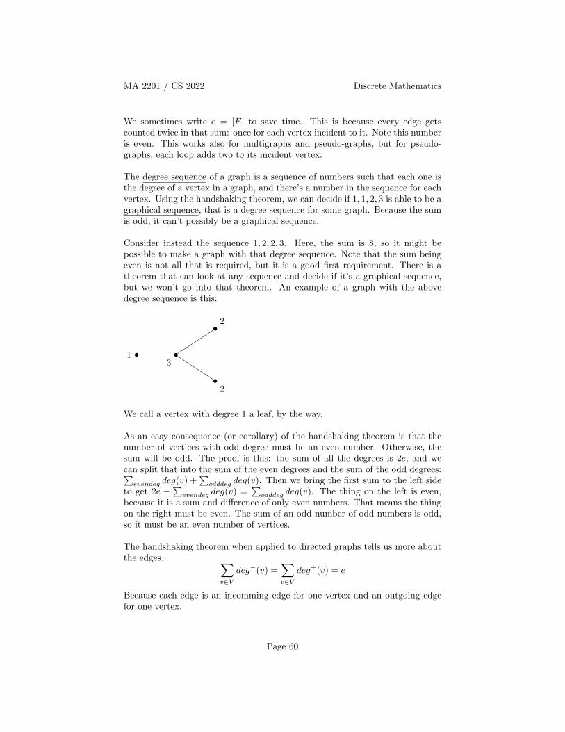
MA 2201 / CS 2022 Discrete Mathematics
We sometimes write e = |E| to save time. This is because every edge getscounted twice in that sum: once for each vertex incident to it. Note this numberis even. This works also for multigraphs and pseudo-graphs, but for pseudo-graphs, each loop adds two to its incident vertex.
The degree sequence of a graph is a sequence of numbers such that each one isthe degree of a vertex in a graph, and there’s a number in the sequence for eachvertex. Using the handshaking theorem, we can decide if 1, 1, 2, 3 is able to be agraphical sequence, that is a degree sequence for some graph. Because the sumis odd, it can’t possibly be a graphical sequence.
Consider instead the sequence 1, 2, 2, 3. Here, the sum is 8, so it might bepossible to make a graph with that degree sequence. Note that the sum beingeven is not all that is required, but it is a good first requirement. There is atheorem that can look at any sequence and decide if it’s a graphical sequence,but we won’t go into that theorem. An example of a graph with the abovedegree sequence is this:
13
2
2
We call a vertex with degree 1 a leaf, by the way.
As an easy consequence (or corollary) of the handshaking theorem is that thenumber of vertices with odd degree must be an even number. Otherwise, thesum will be odd. The proof is this: the sum of all the degrees is 2e, and wecan split that into the sum of the even degrees and the sum of the odd degrees:∑
evendeg deg(v) +∑
odddeg deg(v). Then we bring the first sum to the left sideto get 2e −
∑evendeg deg(v) =
∑odddeg deg(v). The thing on the left is even,
because it is a sum and difference of only even numbers. That means the thingon the right must be even. The sum of an odd number of odd numbers is odd,so it must be an even number of vertices.
The handshaking theorem when applied to directed graphs tells us more aboutthe edges. ∑
v∈Vdeg−(v) =
∑v∈V
deg+(v) = e
Because each edge is an incomming edge for one vertex and an outgoing edgefor one vertex.
Page 60
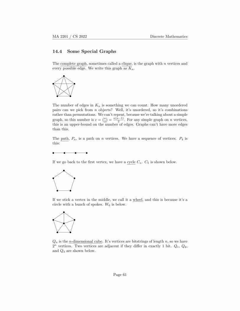
MA 2201 / CS 2022 Discrete Mathematics
14.4 Some Special Graphs
The complete graph, sometimes called a clique, is the graph with n vertices andevery possible edge. We write this graph as Kn.
The number of edges in Kn is something we can count. How many unorderedpairs can we pick from n objects? Well, it’s unordered, so it’s combinationsrather than permutations. We can’t repeat, because we’re talking about a simple
graph, so this number is e =(n2
)= n(n−1)
2 . For any simple graph on n vertices,this is an upper-bound on the number of edges. Graphs can’t have more edgesthan this.
The path, Pn, is a path on n vertices. We have a sequence of vertices. P4 isthis:
If we go back to the first vertex, we have a cycle Cn. C5 is shown below.
If we stick a vertex in the middle, we call it a wheel, and this is because it’s acircle with a bunch of spokes. W6 is below.
Qn is the n-dimensional cube. It’s vertices are bitstrings of length n, so we have2n vertices. Two vertices are adjacent if they differ in exactly 1 bit. Q1, Q2,and Q3 are shown below.
Page 61
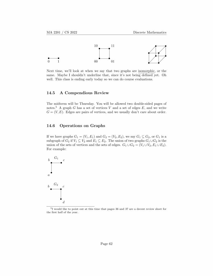
MA 2201 / CS 2022 Discrete Mathematics
0 1 00 01
10 11
Next time, we’ll look at when we say that two graphs are isomorphic, or thesame. Maybe I shouldn’t underline that, since it’s not being defined yet. Ohwell. This class is ending early today so we can do course evaluations.
14.5 A Compendious Review
The midterm will be Thursday. You will be allowed two double-sided pages ofnotes.5 A graph G has a set of vertices V and a set of edges E, and we writeG = (V,E). Edges are pairs of vertices, and we usually don’t care about order.
14.6 Operations on Graphs
If we have graphs G1 = (V1, E1) and G2 = (V2, E2), we say G1 ⊆ G2, or G1 is asubgraph of G2 if V1 ⊆ V2 and E1 ⊆ E2. The union of two graphs G1∪G2 is theunion of the sets of vertices and the sets of edges. G1 ∪G2 = (V1 ∪V2, E1 ∪E2).For example:
a
b cG1
b c
d
G2
5I would like to point out at this time that pages 36 and 37 are a decent review sheet forthe first half of the year.
Page 62
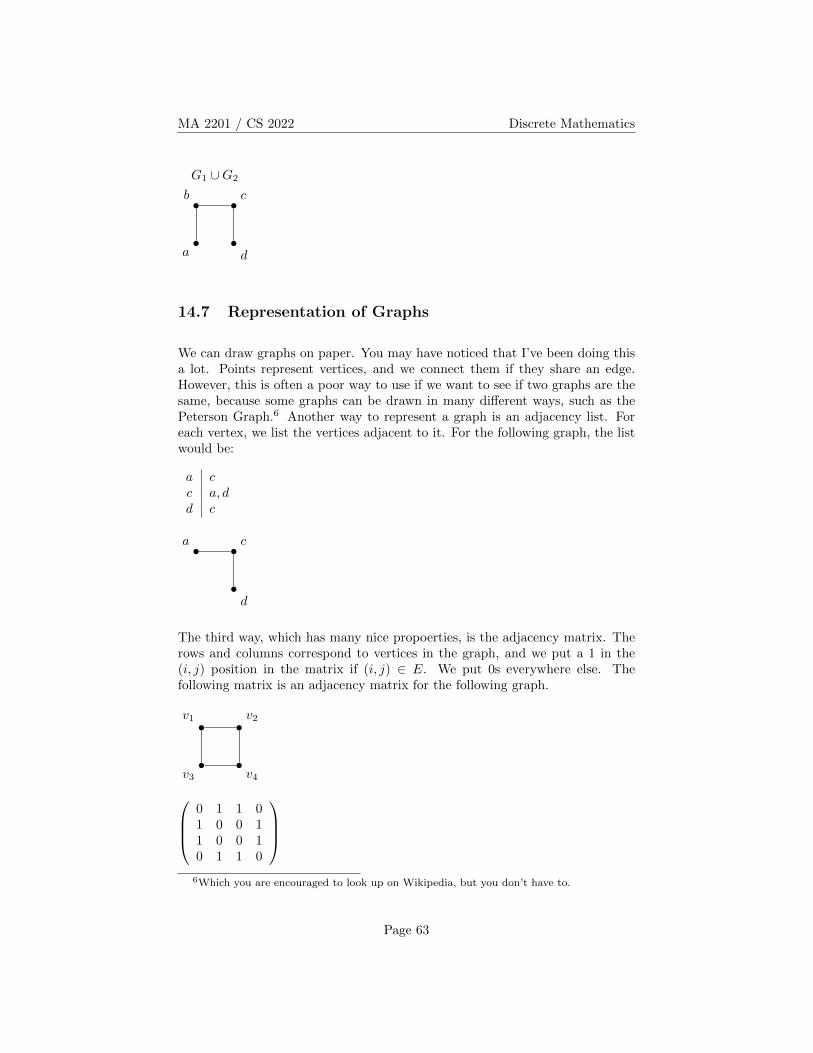
MA 2201 / CS 2022 Discrete Mathematics
a
b c
d
G1 ∪G2
14.7 Representation of Graphs
We can draw graphs on paper. You may have noticed that I’ve been doing thisa lot. Points represent vertices, and we connect them if they share an edge.However, this is often a poor way to use if we want to see if two graphs are thesame, because some graphs can be drawn in many different ways, such as thePeterson Graph.6 Another way to represent a graph is an adjacency list. Foreach vertex, we list the vertices adjacent to it. For the following graph, the listwould be:
a cc a, dd c
a c
d
The third way, which has many nice propoerties, is the adjacency matrix. Therows and columns correspond to vertices in the graph, and we put a 1 in the(i, j) position in the matrix if (i, j) ∈ E. We put 0s everywhere else. Thefollowing matrix is an adjacency matrix for the following graph.
v1 v2
v3 v40 1 1 01 0 0 11 0 0 10 1 1 0
6Which you are encouraged to look up on Wikipedia, but you don’t have to.
Page 63
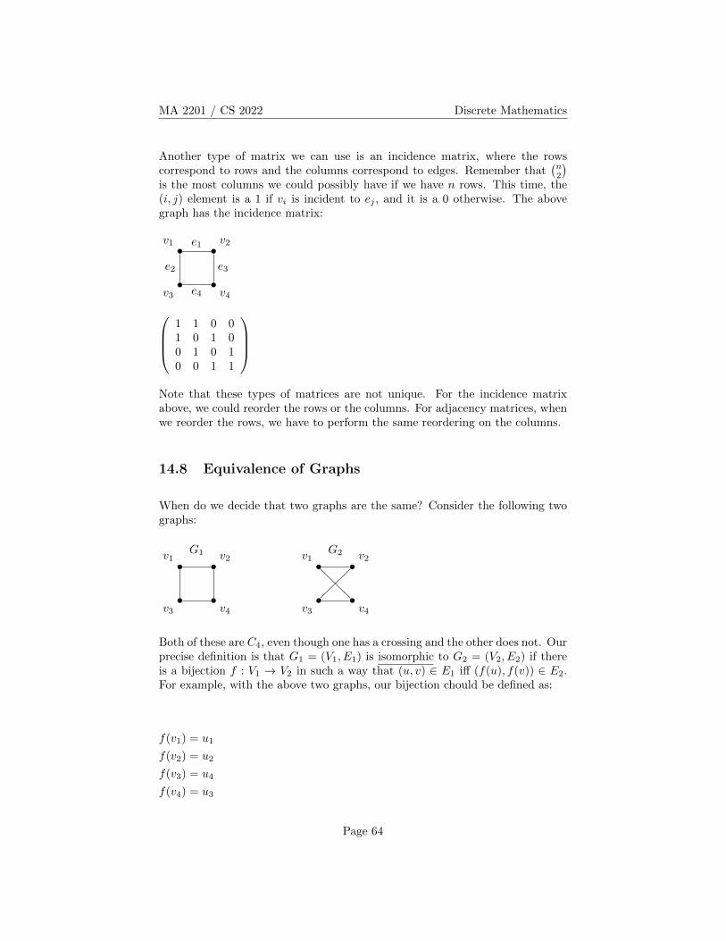
MA 2201 / CS 2022 Discrete Mathematics
Another type of matrix we can use is an incidence matrix, where the rowscorrespond to rows and the columns correspond to edges. Remember that
(n2
)is the most columns we could possibly have if we have n rows. This time, the(i, j) element is a 1 if vi is incident to ej , and it is a 0 otherwise. The abovegraph has the incidence matrix:
v1 v2
v3 v4
e1
e2 e3
e41 1 0 01 0 1 00 1 0 10 0 1 1
Note that these types of matrices are not unique. For the incidence matrixabove, we could reorder the rows or the columns. For adjacency matrices, whenwe reorder the rows, we have to perform the same reordering on the columns.
14.8 Equivalence of Graphs
When do we decide that two graphs are the same? Consider the following twographs:
v1 v2
v3 v4
G1 v1 v2
v3 v4
G2
Both of these are C4, even though one has a crossing and the other does not. Ourprecise definition is that G1 = (V1, E1) is isomorphic to G2 = (V2, E2) if thereis a bijection f : V1 → V2 in such a way that (u, v) ∈ E1 iff (f(u), f(v)) ∈ E2.For example, with the above two graphs, our bijection chould be defined as:
f(v1) = u1
f(v2) = u2
f(v3) = u4
f(v4) = u3
Page 64
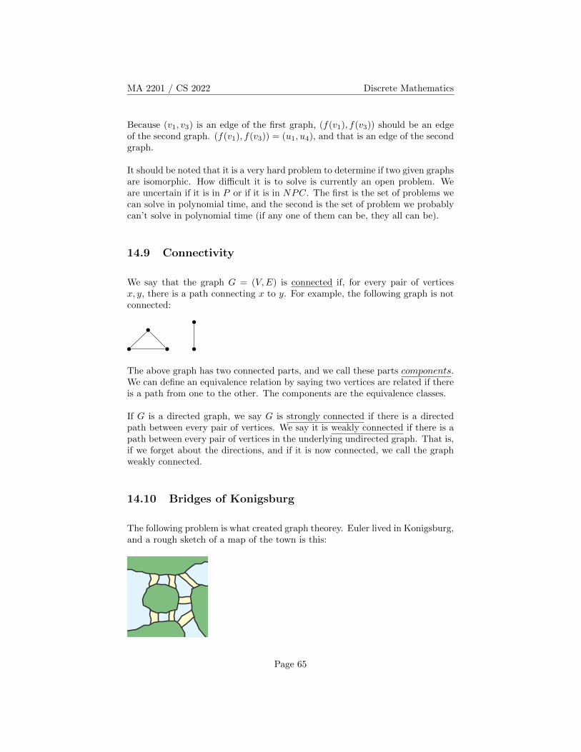
MA 2201 / CS 2022 Discrete Mathematics
Because (v1, v3) is an edge of the first graph, (f(v1), f(v3)) should be an edgeof the second graph. (f(v1), f(v3)) = (u1, u4), and that is an edge of the secondgraph.
It should be noted that it is a very hard problem to determine if two given graphsare isomorphic. How difficult it is to solve is currently an open problem. Weare uncertain if it is in P or if it is in NPC. The first is the set of problems wecan solve in polynomial time, and the second is the set of problem we probablycan’t solve in polynomial time (if any one of them can be, they all can be).
14.9 Connectivity
We say that the graph G = (V,E) is connected if, for every pair of verticesx, y, there is a path connecting x to y. For example, the following graph is notconnected:
The above graph has two connected parts, and we call these parts components.We can define an equivalence relation by saying two vertices are related if thereis a path from one to the other. The components are the equivalence classes.
If G is a directed graph, we say G is strongly connected if there is a directedpath between every pair of vertices. We say it is weakly connected if there is apath between every pair of vertices in the underlying undirected graph. That is,if we forget about the directions, and if it is now connected, we call the graphweakly connected.
14.10 Bridges of Konigsburg
The following problem is what created graph theorey. Euler lived in Konigsburg,and a rough sketch of a map of the town is this:
Page 65
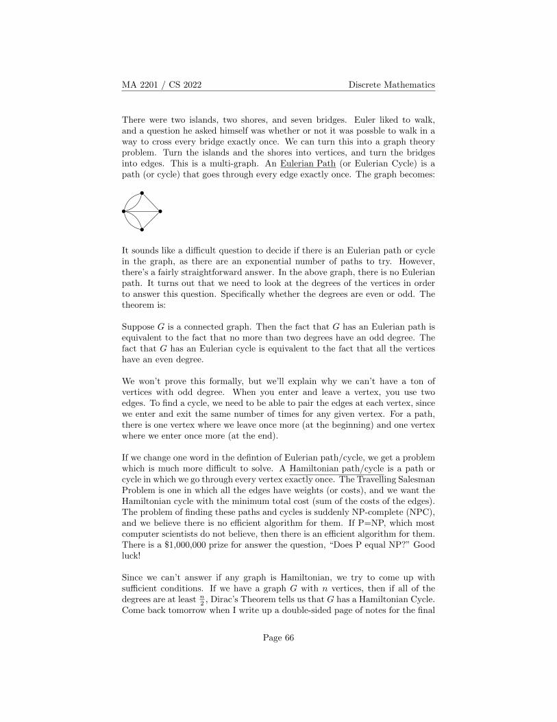
MA 2201 / CS 2022 Discrete Mathematics
There were two islands, two shores, and seven bridges. Euler liked to walk,and a question he asked himself was whether or not it was possble to walk in away to cross every bridge exactly once. We can turn this into a graph theoryproblem. Turn the islands and the shores into vertices, and turn the bridgesinto edges. This is a multi-graph. An Eulerian Path (or Eulerian Cycle) is apath (or cycle) that goes through every edge exactly once. The graph becomes:
It sounds like a difficult question to decide if there is an Eulerian path or cyclein the graph, as there are an exponential number of paths to try. However,there’s a fairly straightforward answer. In the above graph, there is no Eulerianpath. It turns out that we need to look at the degrees of the vertices in orderto answer this question. Specifically whether the degrees are even or odd. Thetheorem is:
Suppose G is a connected graph. Then the fact that G has an Eulerian path isequivalent to the fact that no more than two degrees have an odd degree. Thefact that G has an Eulerian cycle is equivalent to the fact that all the verticeshave an even degree.
We won’t prove this formally, but we’ll explain why we can’t have a ton ofvertices with odd degree. When you enter and leave a vertex, you use twoedges. To find a cycle, we need to be able to pair the edges at each vertex, sincewe enter and exit the same number of times for any given vertex. For a path,there is one vertex where we leave once more (at the beginning) and one vertexwhere we enter once more (at the end).
If we change one word in the defintion of Eulerian path/cycle, we get a problemwhich is much more difficult to solve. A Hamiltonian path/cycle is a path orcycle in which we go through every vertex exactly once. The Travelling SalesmanProblem is one in which all the edges have weights (or costs), and we want theHamiltonian cycle with the minimum total cost (sum of the costs of the edges).The problem of finding these paths and cycles is suddenly NP-complete (NPC),and we believe there is no efficient algorithm for them. If P=NP, which mostcomputer scientists do not believe, then there is an efficient algorithm for them.There is a $1,000,000 prize for answer the question, “Does P equal NP?” Goodluck!
Since we can’t answer if any graph is Hamiltonian, we try to come up withsufficient conditions. If we have a graph G with n vertices, then if all of thedegrees are at least n
2 , Dirac’s Theorem tells us that G has a Hamiltonian Cycle.Come back tomorrow when I write up a double-sided page of notes for the final
Page 66
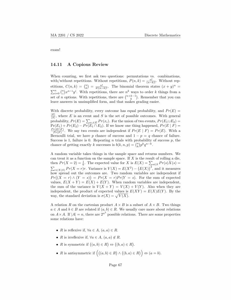
MA 2201 / CS 2022 Discrete Mathematics
exam!
14.11 A Copious Review
When counting, we first ask two questions: permutations vs. combinations,with/without repetitions. Without repetitions, P (n, k) = n!
(n−k)! . Without rep-
etitions, C(n, k) =(nk
)= n!
k!(n−k)! . The binomial theorem states (x + y)n =∑ni=0
(ni
)xn−iyi. With repetitions, there are nk ways to order k things from a
set of n options. With repetitions, there are(n+k−1
k
). Remember that you can
leave answers in unsimplified form, and that makes grading easier.
With discrete probability, every outcome has equal probability, and Pr(E) =|E||S| , where E is an event and S is the set of possible outcomes. With general
probability, Pr(E) =∑
xi∈E Pr(xi). For the union of two events, Pr(E1∪E2) =Pr(E1) +Pr(E2)−Pr(E1 ∩E2). If we know one thing happened, Pr(E | F ) =Pr(E∩F )Pr(F ) . We say two events are independent if Pr(E | F ) = Pr(E). With a
Bernoulli trial, we have p chance of success and 1 − p = q chance of failure.Success is 1, failure is 0. Repeating n trials with probability of success p, thechance of getting exactly k successes is b(k, n, p) =
(nk
)pkqn−k.
A random variable takes things in the sample space and returns numbers. Wecan treat it as a function on the sample space. If X is the result of rolling a die,then Pr(X = 2) = 1
6 . The expected value for X is E(X) =∑
s∈S Pr(s)X(s) =∑r∈X(S) Pr(X = r)r. Variance is V (X) = E(X2)−
(E(X)
)2, and it measures
how spread out the outcomes are. Two random variables are independent ifPr((X = r) ∧ (Y = s)
)= Pr(X = r)Pr(Y = s). For the sum of expected
values, E(X + Y ) = E(X) + E(Y ). When random variables are independent,the sum of the variance is V (X + Y ) = V (X) + V (Y ). Also when they areindependent, the product of expected values is E(XY ) = E(X)E(Y ). By theway, the standard deviation is σ(X) =
√V (X).
A relation R on the cartesian product A×B is a subset of A×B. Two thingsa ∈ A and b ∈ B are related if (a, b) ∈ R. We usually care more about relations
on A×A. If |A| = n, there are 2n2
possible relations. There are some propertiessome relations have:
• R is reflexive if, ∀a ∈ A, (a, a) ∈ R.
• R is irreflexive if, ∀a ∈ A, (a, a) 6∈ R.
• R is symmetric if((a, b) ∈ R
)⇔((b, a) ∈ R
).
• R is antisymmetric if((
(a, b) ∈ R)∧((b, a) ∈ R
))⇔ (a = b).
Page 67
MA 2201 / CS 2022 Discrete Mathematics
• R is transitive if((
(a, b) ∈ R)∧((b, c) ∈ R
))⇔((a, c) ∈ R
)An equivalence relation is a relation that is reflexive, symmetric, and transitive.A partial ordering is a relation that is reflexive, antisymmetric, and transitive.The closure of a relation R under a property P (from the above list) is a newrelation R′ such that R ⊆ R′, R′ has the property P , and R′ is the smallest setthat satisfies those two conditions.
When we talk about graphs, we talk about vertices (points) and edges (lineswhich might bend). Simple graphs have no more than once edge joining anytwo vertices and no edges that join a vertex to itself. Also, the edges have nodirection. A directed graph has edges which go from one vertex to another.The degree of a vertex is the number of edges incident to it, or the number ofvertices adjacent to it. Complete graphs Kn have n vertices and all possibleedges. Paths Pn have n vertices connected in a sequence with two vertices ofdegree 1 and all others of degree 2. Cycles Cn are paths with an edge connectingthe two vertices of degree 1.
Because graphs are sets of vertices and edges, we can look at unions and inter-sections of them, and we can look at subsets of them. A graph is connected ifthere is a path connecting any two vertices.
Two graphs are equivalent if there is a bijection f between the vertices such thatwhen (u, v) is an edge in the first graph, (f(u), f(v)) is an edge in the secondgraph, and there are no other edges in the second graph.
A degree sequence is a set of numbers which are the degrees of vertices in agraph. A graph with n vertices will have n numbers in the sequence. If the sumof these numbers is odd, there is no graph with that degree sequence.
Page 68