Embed Size (px)
Citation preview
DiscreteInferenceandLearningLecture3
MVA2017–2018
h<p://thoth.inrialpes.fr/~alahari/disinflearn
SlidesbasedonmaterialfromPushmeetKohli,NikosKomodakis,M.PawanKumar

Recap
The st-mincut problem
What problems can we solve using st-mincut?
st-mincut based Move algorithms
Connection between st-mincut and energy minimization?

St-mincut based Move algorithms
• Commonly used for solving non-submodular multi-label problems
• Extremely efficient and produce good solutions
• Not Exact: Produce local optima
E(y) = ∑ θi (yi) + ∑ θij (yi,yj) i,j i
y ϵ Labels L = {l1, l2, … , lk}

Move Making Algorithms
Search Neighbourhood
Current Solution
Optimal Move
Solution Space
Ene
rgy

Move Making Algorithms
Search Neighbourhood
Current Solution
Optimal Move
Solution Space
Ene
rgy

Computing the Optimal Move
Search Neighbourhood
Current Solution
Optimal Move
yc (t) Key Property
Move Space
Bigger move space
Solution Space
Ene
rgy
• Better solutions • Finding the optimal move hard

Moves using Graph Cuts
Expansion and Swap move algorithms [Boykov Veksler and Zabih, PAMI 2001]
• Makes a series of changes to the solution (moves) • Each move results in a solution with smaller energy
Space of Solutions (y) : LN
Move Space (t) : 2N
Search Neighbourhood
Current Solution
N Number of Variables
L Number of Labels

Moves using Graph Cuts
Expansion and Swap move algorithms [Boykov Veksler and Zabih, PAMI 2001]
• Makes a series of changes to the solution (moves) • Each move results in a solution with smaller energy
Current Solution
Construct a move function
Minimize move function to get optimal move
Move to new solution
How to minimize
move functions?

General Binary Moves
Minimize over move variables t to get the optimal move
y = t y1 + (1- t) y2 New
solution Current Solution
Second solution
Em(t) = E(t y1 + (1- t) y2)
Boykov, Veksler and Zabih, PAMI 2001
Move energy is a submodular QPBF (Exact Minimization Possible)

Expansion Move
Sky House
Tree Ground
Initialize with Tree Status:
[Boykov, Veksler, Zabih] [Boykov, Veksler, Zabih]
• Variables take label α or retain current label

Expansion Move
Sky House
Tree Ground
Status: Expand Ground
[Boykov, Veksler, Zabih] [Boykov, Veksler, Zabih]
• Variables take label α or retain current label

Expansion Move
Sky House
Tree Ground
Status: Expand House
[Boykov, Veksler, Zabih] [Boykov, Veksler, Zabih]
• Variables take label α or retain current label

Expansion Move
Sky House
Tree Ground
Status: Expand Sky
[Boykov, Veksler, Zabih] [Boykov, Veksler, Zabih]
• Variables take label α or retain current label

Expansion Move
• Move energy is submodular if: – Unary Potentials: Arbitrary – Pairwise potentials: Metric
[Boykov, Veksler, Zabih] [Boykov, Veksler, Zabih]
Semi metric
• Variables take label α or retain current label
Examples: Potts model, Truncated linear Cannot solve truncated quadratic
θij (la,lb) ≥ 0
θij (la,lb) = 0 iff a = b

Expansion Move
• Move energy is submodular if: – Unary Potentials: Arbitrary – Pairwise potentials: Metric
[Boykov, Veksler, Zabih] [Boykov, Veksler, Zabih]
θij (la,lb) + θij (lb,lc) ≥ θij (la,lc) Triangle
Inequality
• Variables take label α or retain current label
Examples: Potts model, Truncated linear Cannot solve truncated quadratic

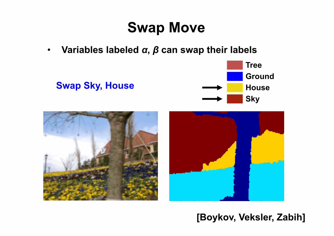
Swap Move
Sky House
Tree Ground
Swap Sky, House
[Boykov, Veksler, Zabih]
• Variables labeled α, β can swap their labels
Swap Move
Sky House
Tree Ground
Swap Sky, House
[Boykov, Veksler, Zabih]
• Variables labeled α, β can swap their labels

Swap Move • Variables labeled α, β can swap their labels
• Move energy is submodular if: – Unary Potentials: Arbitrary – Pairwise potentials: Semimetric
[Boykov, Veksler, Zabih]
θij (la,lb) ≥ 0
θij (la,lb) = 0 a = b
Examples: Potts model, Truncated Convex

Exact Transformation
(global optimum)
Or Relaxed transformation
(partially optimal)
Summary
T
S st-mincut
Labelling Problem
Submodular Quadratic Pseudoboolean Function
Move making algorithms
Sub-problem

Where do we stand ?
Chain/Tree, 2/multi-label: Use BP
Grid graph - submodular, 2-label: Use graphcuts “metric”: Use expansion otherwise: Use TRW, dual decomposition, relaxation

Dynamic Energy Minimization

Image Segmentation in Video
Video frame Flow Global Optimum
pqw
n-links st-cut s
t
= 0
= 1
E(x) x*

Image Segmentation in Video
Video frame
Flow Global Optimum

Dynamic Energy Minimization
EB SB computationally
expensive operation
EA SA minimize
Recycling Solutions
Can we do better?
Boykov & Jolly ICCV’01, Kohli & Torr (ICCV05, PAMI07)

Dynamic Energy Minimization
EB SB computationally
expensive operation
EA SA minimize
cheaper operation
Simpler energy
EB* differences
between A and B
A and B similar
Kohli & Torr (ICCV05, PAMI07)
Reparametrization
Reuse flow
Boykov & Jolly ICCV’01, Kohli & Torr (ICCV05, PAMI07)

Reparameterized Energy
Dynamic Energy Minimization
Kohli & Torr (ICCV05, PAMI07) Boykov & Jolly ICCV’01, Kohli & Torr (ICCV05, PAMI07)
E(a1,a2) = 2a1 + 5ā1+ 9a2 + 4ā2 + 2a1ā2 + ā1a2
E(a1,a2) = 8 + ā1+ 3a2 + 3ā1a2
Original Energy
E(a1,a2) = 2a1 + 5ā1+ 9a2 + 4ā2 + 7a1ā2 + ā1a2
E(a1,a2) = 8 + ā1+ 3a2 + 3ā1a2 + 5a1ā2
New Energy
New Reparameterized Energy
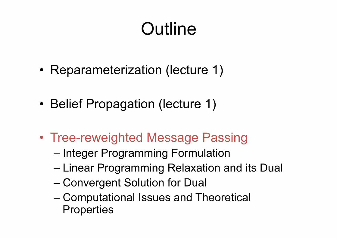
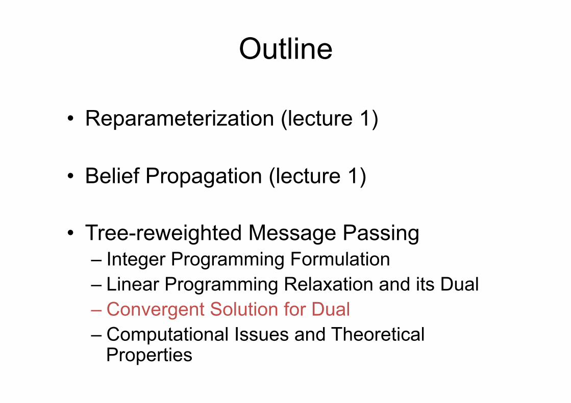
Outline • Reparameterization (lecture 1)
• Belief Propagation (lecture 1) • Tree-reweighted Message Passing
– Integer Programming Formulation – Linear Programming Relaxation and its Dual – Convergent Solution for Dual – Computational Issues and Theoretical
Properties

First…
RecapofIntegerLinearProgram

IntegerLinearProgram
s.t.Ax≤b
maxxcTx
xisanintegervector
Everyelementofxisaninteger

IntegerLinearProgram
s.t.Ax≤b
maxxcTx
x∈Zn
Everyelementofxisaninteger

Example
4x1–x2≤8
maxxx1+x2
2x1+x2≤10
5x1-2x2≥-2
x1≥0
x2≥0
s.t.
x∈Zn
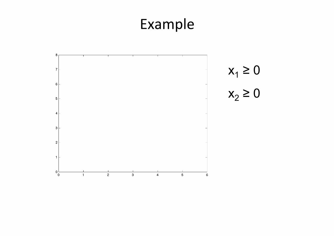
Example
x1 ≥ 0
x2 ≥ 0

Example
4x1 – x2 = 8
x1 ≥ 0
x2 ≥ 0

Example
4x1 – x2 ≤ 8
x1 ≥ 0
x2 ≥ 0

Example
4x1 – x2 ≤ 8
2x1 + x2 ≤ 10
5x1 - 2x2 ≥ -2
x1 ≥ 0
x2 ≥ 0

Example
4x1 – x2 ≤ 8
2x1 + x2 ≤ 10
5x1 - 2x2 ≥ -2
x1 ≥ 0
x2 ≥ 0
x∈Zn
maxxcTx
(2,6)
(3,4)
(2,0)(0,0)
(0,1)

Example
4x1 – x2 ≤ 8
2x1 + x2 ≤ 10
5x1 - 2x2 ≥ -2
x1 ≥ 0
x2 ≥ 0
x∈Zn
maxxcTx
(2,6)
(3,4)
(2,0)(0,0)
(0,1)
Why? Trueingeneral?
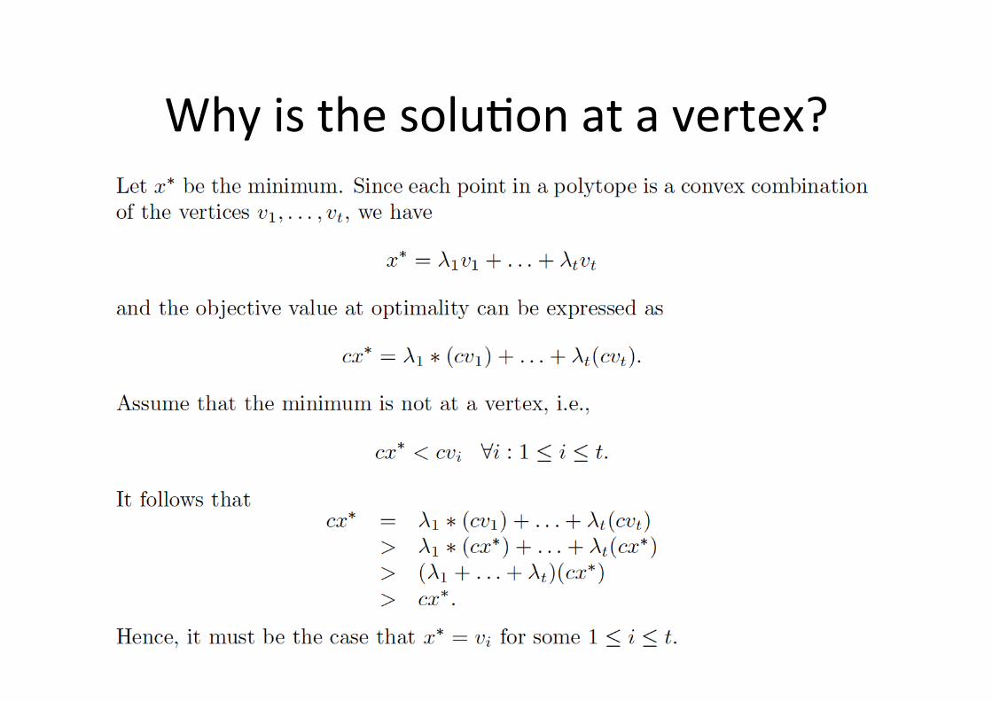
Whyisthesoluaonatavertex?
Integer Programming Formulation
Va Vb
Label l0
Label l12
5
4
2
0
1 1
0
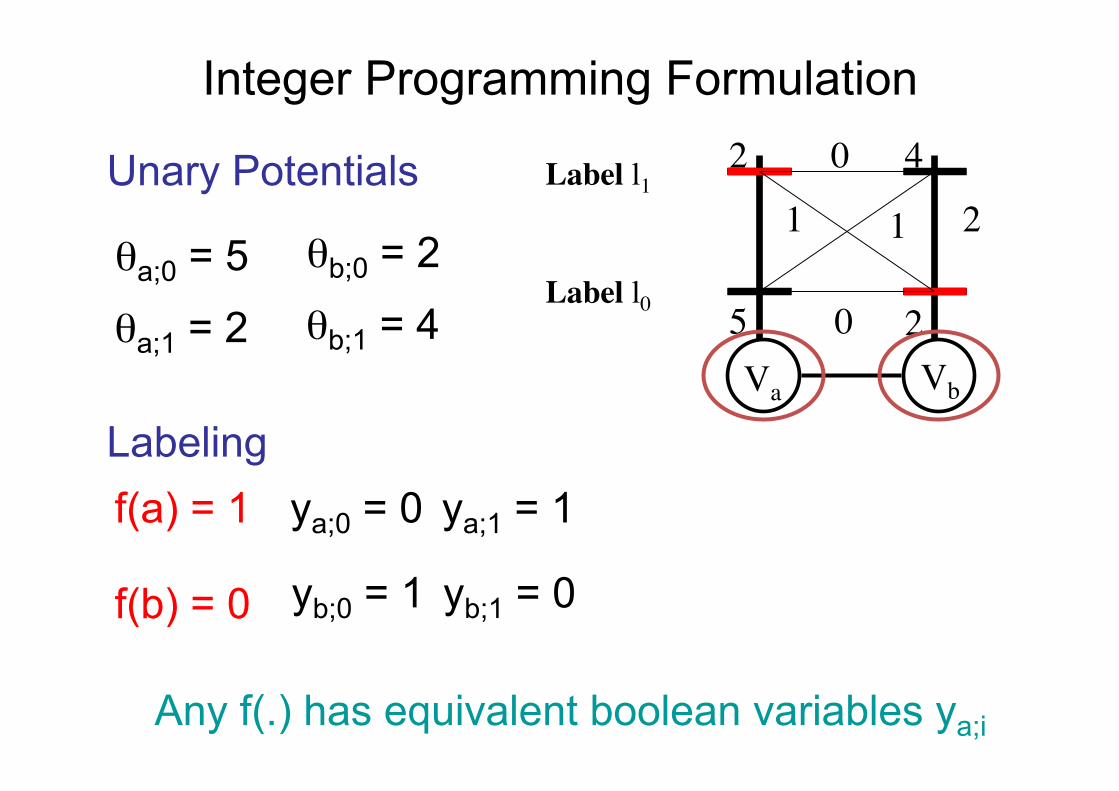
2Unary Potentials
θa;0 = 5
θa;1 = 2
θb;0 = 2
θb;1 = 4
Labeling f(a) = 1
f(b) = 0
ya;0 = 0 ya;1 = 1
yb;0 = 1 yb;1 = 0
Any f(.) has equivalent boolean variables ya;i

Integer Programming Formulation
Va Vb
2
5
4
2
0
1 1
0
2Unary Potentials
θa;0 = 5
θa;1 = 2
θb;0 = 2
θb;1 = 4
Labeling f(a) = 1
f(b) = 0
ya;0 = 0 ya;1 = 1
yb;0 = 1 yb;1 = 0
Find the optimal variables ya;i
Label l0
Label l1

Integer Programming Formulation
Va Vb
2
5
4
2
0
1 1
0
2Unary Potentials
θa;0 = 5
θa;1 = 2
θb;0 = 2
θb;1 = 4
Sum of Unary Potentials
∑a ∑i θa;i ya;i
ya;i ∈ {0,1}, for all Va, li ∑i ya;i = 1, for all Va
Label l0
Label l1

Integer Programming Formulation
Va Vb
2
5
4
2
0
1 1
0
2Pairwise Potentials
θab;00 = 0
θab;10 = 1
θab;01 = 1
θab;11 = 0
Sum of Pairwise Potentials
∑(a,b) ∑ik θab;ik ya;iyb;k
ya;i ∈ {0,1} ∑i ya;i = 1
Label l0
Label l1

Integer Programming Formulation
Va Vb
2
5
4
2
0
1 1
0
2Pairwise Potentials
θab;00 = 0
θab;10 = 1
θab;01 = 1
θab;11 = 0
Sum of Pairwise Potentials
∑(a,b) ∑ik θab;ik yab;ik
ya;i ∈ {0,1} ∑i ya;i = 1
yab;ik = ya;i yb;k
Label l0
Label l1

Integer Programming Formulation
min ∑a ∑i θa;i ya;i + ∑(a,b) ∑ik θab;ik yab;ik
ya;i ∈ {0,1}
∑i ya;i = 1
yab;ik = ya;i yb;k

Integer Programming Formulation
min θTy
ya;i ∈ {0,1}
∑i ya;i = 1
yab;ik = ya;i yb;k
θ = [ … θa;i …. ; … θab;ik ….] y = [ … ya;i …. ; … yab;ik ….]

Integer Programming Formulation
min θTy
ya;i ∈ {0,1}
∑i ya;i = 1
yab;ik = ya;i yb;k
Solve to obtain MAP labeling y*

Integer Programming Formulation
min θTy
ya;i ∈ {0,1}
∑i ya;i = 1
yab;ik = ya;i yb;k
But we can’t solve it in general

Outline • Reparameterization (lecture 1)
• Belief Propagation (lecture 1) • Tree-reweighted Message Passing
– Integer Programming Formulation – Linear Programming Relaxation and its Dual – Convergent Solution for Dual – Computational Issues and Theoretical
Properties

Linear Programming Relaxation
min θTy
ya;i ∈ {0,1}
∑i ya;i = 1
yab;ik = ya;i yb;k
Two reasons why we can’t solve this

Linear Programming Relaxation
min θTy
ya;i ∈ [0,1]
∑i ya;i = 1
yab;ik = ya;i yb;k
One reason why we can’t solve this

Linear Programming Relaxation
min θTy
ya;i ∈ [0,1]
∑i ya;i = 1
∑k yab;ik = ∑kya;i yb;k
One reason why we can’t solve this

Linear Programming Relaxation
min θTy
ya;i ∈ [0,1]
∑i ya;i = 1
One reason why we can’t solve this
= 1 ∑k yab;ik = ya;i∑k yb;k

Linear Programming Relaxation
min θTy
ya;i ∈ [0,1]
∑i ya;i = 1
∑k yab;ik = ya;i
One reason why we can’t solve this

Linear Programming Relaxation
min θTy
ya;i ∈ [0,1]
∑i ya;i = 1
∑k yab;ik = ya;i
No reason why we can’t solve this * *memory requirements, time complexity

Dual of the LP Relaxation Wainwright et al., 2001
Va Vb Vc
Vd Ve Vf
Vg Vh Vi
θ
min θTy
ya;i ∈ [0,1]
∑i ya;i = 1
∑k yab;ik = ya;i

Dual of the LP Relaxation Wainwright et al., 2001
Va Vb Vc
Vd Ve Vf
Vg Vh Vi
θ
Va Vb Vc
Vd Ve Vf
Vg Vh Vi
Va Vb Vc
Vd Ve Vf
Vg Vh Vi
ρ1
ρ2
ρ3
ρ4 ρ5 ρ6
θ1
θ2
θ3 θ4 θ5 θ6
∑ ρiθi = θ
ρi ≥ 0

Dual of the LP Relaxation Wainwright et al., 2001
ρ1
ρ2
ρ3
ρ4 ρ5 ρ6
q*(θ1)
∑ ρiθi = θ
q*(θ2)
q*(θ3) q*(θ4) q*(θ5) q*(θ6)
∑ ρi q*(θi)
Dual of LP
θ
Va Vb Vc
Vd Ve Vf
Vg Vh Vi
Va Vb Vc
Vd Ve Vf
Vg Vh Vi
Va Vb Vc
Vd Ve Vf
Vg Vh Vi
ρi ≥ 0
max

Dual of the LP Relaxation Wainwright et al., 2001
ρ1
ρ2
ρ3
ρ4 ρ5 ρ6
q*(θ1)
∑ ρiθi ≡ θ
q*(θ2)
q*(θ3) q*(θ4) q*(θ5) q*(θ6)
Dual of LP
θ
Va Vb Vc
Vd Ve Vf
Vg Vh Vi
Va Vb Vc
Vd Ve Vf
Vg Vh Vi
Va Vb Vc
Vd Ve Vf
Vg Vh Vi
ρi ≥ 0
∑ ρi q*(θi) max

Dual of the LP Relaxation Wainwright et al., 2001
∑ ρiθi ≡ θ
max ∑ ρi q*(θi)
I can easily compute q*(θi)
I can easily maintain reparam constraint
So can I easily solve the dual?
Outline • Reparameterization (lecture 1)
• Belief Propagation (lecture 1) • Tree-reweighted Message Passing
– Integer Programming Formulation – Linear Programming Relaxation and its Dual – Convergent Solution for Dual – Computational Issues and Theoretical
Properties

TRW Message Passing Kolmogorov, 2006
Va Vb Vc
Vd Ve Vf
Vg Vh Vi
Va Vb Vc
Vd Ve Vf
Vg Vh Vi
ρ1
ρ2
ρ3
θ1
θ2
θ3
θ4 θ5 θ6
ρ4 ρ5 ρ6
∑ ρiθi ≡ θ ∑ ρi
q*(θi)
Pick a variable Va

TRW Message Passing Kolmogorov, 2006
∑ ρiθi ≡ θ ∑ ρi
q*(θi)
Vc Vb Va
θ1c;0
θ1c;1
θ1b;0
θ1b;1
θ1a;0
θ1a;1
Va Vd Vg
θ4a;0
θ4a;1
θ4d;0
θ4d;1
θ4g;0
θ4g;1

TRW Message Passing Kolmogorov, 2006
ρ1θ1 + ρ4θ4 + θrest ≡ θ ρ1
q*(θ1) + ρ4 q*(θ4) + K
Vc Vb Va Va Vd Vg
Reparameterize to obtain min-marginals of Va
θ1c;0
θ1c;1
θ1b;0
θ1b;1
θ1a;0
θ1a;1
θ4a;0
θ4a;1
θ4d;0
θ4d;1
θ4g;0
θ4g;1

TRW Message Passing Kolmogorov, 2006
ρ1θ’1 + ρ4θ’4 + θrest
Vc Vb Va
θ’1c;0
θ’1c;1
θ’1b;0
θ’1b;1
θ’1a;0
θ’1a;1
Va Vd Vg
θ’4a;0
θ’4a;1
θ’4d;0
θ’4d;1
θ’4g;0
θ’4g;1
One pass of Belief Propagation
ρ1 q*(θ’1) + ρ4
q*(θ’4) + K

TRW Message Passing Kolmogorov, 2006
ρ1θ’1 + ρ4θ’4 + θrest ≡ θ
Vc Vb Va Va Vd Vg
Remain the same
ρ1 q*(θ’1) + ρ4
q*(θ’4) + K
θ’1c;0
θ’1c;1
θ’1b;0
θ’1b;1
θ’1a;0
θ’1a;1
θ’4a;0
θ’4a;1
θ’4d;0
θ’4d;1
θ’4g;0
θ’4g;1

TRW Message Passing Kolmogorov, 2006
ρ1θ’1 + ρ4θ’4 + θrest ≡ θ
ρ1 min{θ’1a;0,θ’1a;1} + ρ4
min{θ’4a;0,θ’4a;1} + K
Vc Vb Va Va Vd Vg
θ’1c;0
θ’1c;1
θ’1b;0
θ’1b;1
θ’1a;0
θ’1a;1
θ’4a;0
θ’4a;1
θ’4d;0
θ’4d;1
θ’4g;0
θ’4g;1

TRW Message Passing Kolmogorov, 2006
ρ1θ’1 + ρ4θ’4 + θrest ≡ θ
Vc Vb Va Va Vd Vg
Compute weighted average of min-marginals of Va
θ’1c;0
θ’1c;1
θ’1b;0
θ’1b;1
θ’1a;0
θ’1a;1
θ’4a;0
θ’4a;1
θ’4d;0
θ’4d;1
θ’4g;0
θ’4g;1
ρ1 min{θ’1a;0,θ’1a;1} + ρ4
min{θ’4a;0,θ’4a;1} + K

TRW Message Passing Kolmogorov, 2006
ρ1θ’1 + ρ4θ’4 + θrest ≡ θ
Vc Vb Va Va Vd Vg
θ’’a;0 = ρ1θ’1a;0+ ρ4θ’4a;0
ρ1 + ρ4
θ’’a;1 = ρ1θ’1a;1+ ρ4θ’4a;1
ρ1 + ρ4
θ’1c;0
θ’1c;1
θ’1b;0
θ’1b;1
θ’1a;0
θ’1a;1
θ’4a;0
θ’4a;1
θ’4d;0
θ’4d;1
θ’4g;0
θ’4g;1
ρ1 min{θ’1a;0,θ’1a;1} + ρ4
min{θ’4a;0,θ’4a;1} + K

TRW Message Passing Kolmogorov, 2006
ρ1θ’’1 + ρ4θ’’4 + θrest
Vc Vb Va Va Vd Vg
θ’1c;0
θ’1c;1
θ’1b;0
θ’1b;1
θ’’a;0
θ’’a;1
θ’’a;0
θ’’a;1
θ’4d;0
θ’4d;1
θ’4g;0
θ’4g;1
ρ1 min{θ’1a;0,θ’1a;1} + ρ4
min{θ’4a;0,θ’4a;1} + K
θ’’a;0 = ρ1θ’1a;0+ ρ4θ’4a;0
ρ1 + ρ4
θ’’a;1 = ρ1θ’1a;1+ ρ4θ’4a;1
ρ1 + ρ4

TRW Message Passing Kolmogorov, 2006
ρ1θ’’1 + ρ4θ’’4 + θrest ≡ θ
Vc Vb Va Va Vd Vg
θ’1c;0
θ’1c;1
θ’1b;0
θ’1b;1
θ’’a;0
θ’’a;1
θ’’a;0
θ’’a;1
θ’4d;0
θ’4d;1
θ’4g;0
θ’4g;1
ρ1 min{θ’1a;0,θ’1a;1} + ρ4
min{θ’4a;0,θ’4a;1} + K
θ’’a;0 = ρ1θ’1a;0+ ρ4θ’4a;0
ρ1 + ρ4
θ’’a;1 = ρ1θ’1a;1+ ρ4θ’4a;1
ρ1 + ρ4
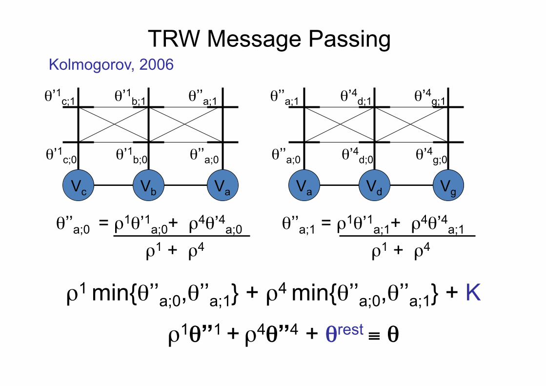
TRW Message Passing Kolmogorov, 2006
ρ1θ’’1 + ρ4θ’’4 + θrest ≡ θ
Vc Vb Va Va Vd Vg
ρ1 min{θ’’a;0,θ’’a;1} + ρ4
min{θ’’a;0,θ’’a;1} + K
θ’1c;0
θ’1c;1
θ’1b;0
θ’1b;1
θ’’a;0
θ’’a;1
θ’’a;0
θ’’a;1
θ’4d;0
θ’4d;1
θ’4g;0
θ’4g;1
θ’’a;0 = ρ1θ’1a;0+ ρ4θ’4a;0
ρ1 + ρ4
θ’’a;1 = ρ1θ’1a;1+ ρ4θ’4a;1
ρ1 + ρ4

TRW Message Passing Kolmogorov, 2006
ρ1θ’’1 + ρ4θ’’4 + θrest ≡ θ
Vc Vb Va Va Vd Vg
(ρ1 + ρ4) min{θ’’a;0, θ’’a;1} + K
θ’1c;0
θ’1c;1
θ’1b;0
θ’1b;1
θ’’a;0
θ’’a;1
θ’’a;0
θ’’a;1
θ’4d;0
θ’4d;1
θ’4g;0
θ’4g;1
θ’’a;0 = ρ1θ’1a;0+ ρ4θ’4a;0
ρ1 + ρ4
θ’’a;1 = ρ1θ’1a;1+ ρ4θ’4a;1
ρ1 + ρ4

TRW Message Passing Kolmogorov, 2006
ρ1θ’’1 + ρ4θ’’4 + θrest ≡ θ
Vc Vb Va Va Vd Vg
(ρ1 + ρ4) min{θ’’a;0, θ’’a;1} + K
θ’1c;0
θ’1c;1
θ’1b;0
θ’1b;1
θ’’a;0
θ’’a;1
θ’’a;0
θ’’a;1
θ’4d;0
θ’4d;1
θ’4g;0
θ’4g;1
min {p1+p2, q1+q2} min {p1, q1} + min {p2, q2} ≥

TRW Message Passing Kolmogorov, 2006
ρ1θ’’1 + ρ4θ’’4 + θrest ≡ θ
Vc Vb Va Va Vd Vg
Objective function increases or remains constant
θ’1c;0
θ’1c;1
θ’1b;0
θ’1b;1
θ’’a;0
θ’’a;1
θ’’a;0
θ’’a;1
θ’4d;0
θ’4d;1
θ’4g;0
θ’4g;1
(ρ1 + ρ4) min{θ’’a;0, θ’’a;1} + K

TRW Message Passing
Initialize θi. Take care of reparam constraint
Choose random variable Va
Compute min-marginals of Va for all trees
Node-average the min-marginals
REPEAT
Kolmogorov, 2006
Can also do edge-averaging

Example 1
Va Vb
0
1 1
0
2
5
4
2l0
l1
Vb Vc
0
2 3
1
4
2
6
3Vc Va
1
4 1
0
6
3
6
4
ρ2 =1 ρ3 =1 ρ1 =1
5 6 7
Pick variable Va. Reparameterize.

Example 1
Va Vb
-3
-2 -1
-2
5
7
4
2Vb Vc
0
2 3
1
4
2
6
3Vc Va
-3
1 -3
-3
6
3
10
7
ρ2 =1 ρ3 =1 ρ1 =1
5 6 7
Average the min-marginals of Va
l0
l1

Example 1
Va Vb
-3
-2 -1
-2
7.5
7
4
2Vb Vc
0
2 3
1
4
2
6
3Vc Va
-3
1 -3
-3
6
3
7.5
7
ρ2 =1 ρ3 =1 ρ1 =1
7 6 7
Pick variable Vb. Reparameterize.
l0
l1

Example 1
Va Vb
-7.5
-7 -5.5
-7
7.5
7
8.5
7Vb Vc
-5
-3 -1
-3
9
6
6
3Vc Va
-3
1 -3
-3
6
3
7.5
7
ρ2 =1 ρ3 =1 ρ1 =1
7 6 7
Average the min-marginals of Vb
l0
l1

Example 1
Va Vb
-7.5
-7 -5.5
-7
7.5
7
8.75
6.5Vb Vc
-5
-3 -1
-3
8.75
6.5
6
3Vc Va
-3
1 -3
-3
6
3
7.5
7
ρ2 =1 ρ3 =1 ρ1 =1
6.5 6.5 7 Value of dual does not increase
l0
l1

Example 1
Va Vb
-7.5
-7 -5.5
-7
7.5
7
8.75
6.5Vb Vc
-5
-3 -1
-3
8.75
6.5
6
3Vc Va
-3
1 -3
-3
6
3
7.5
7
ρ2 =1 ρ3 =1 ρ1 =1
6.5 6.5 7 Maybe it will increase for Vc
NO
l0
l1

Example 1
Va Vb
-7.5
-7 -5.5
-7
7.5
7
8.75
6.5Vb Vc
-5
-3 -1
-3
8.75
6.5
6
3Vc Va
-3
1 -3
-3
6
3
7.5
7
ρ2 =1 ρ3 =1 ρ1 =1
Strong Tree Agreement
Exact MAP Estimate
f1(a) = 0 f1(b) = 0 f2(b) = 0 f2(c) = 0 f3(c) = 0 f3(a) = 0
l0
l1

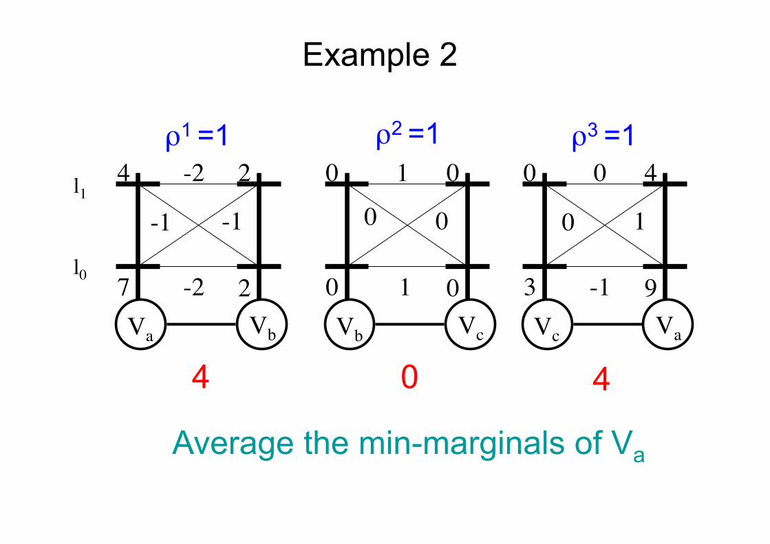
Example 2
Va Vb
0
1 1
0
2
5
2
2Vb Vc
1
0 0
1
0
0
0
0Vc Va
0
1 1
0
0
3
4
8
ρ2 =1 ρ3 =1 ρ1 =1
4 0 4
Pick variable Va. Reparameterize.
l0
l1
Example 2
Va Vb
-2
-1 -1
-2
4
7
2
2Vb Vc
1
0 0
1
0
0
0
0Vc Va
0
0 1
-1
0
3
4
9
ρ2 =1 ρ3 =1 ρ1 =1
4 0 4
Average the min-marginals of Va
l0
l1

Example 2
Va Vb
-2
-1 -1
-2
4
8
2
2Vb Vc
1
0 0
1
0
0
0
0Vc Va
0
0 1
-1
0
3
4
8
ρ2 =1 ρ3 =1 ρ1 =1
4 0 4 Value of dual does not increase
l0
l1

Example 2
Va Vb
-2
-1 -1
-2
4
8
2
2Vb Vc
1
0 0
1
0
0
0
0Vc Va
0
0 1
-1
0
3
4
8
ρ2 =1 ρ3 =1 ρ1 =1
4 0 4 Maybe it will decrease for Vb or Vc
NO
l0
l1

Example 2
Va Vb
-2
-1 -1
-2
4
8
2
2Vb Vc
1
0 0
1
0
0
0
0Vc Va
0
0 1
-1
0
3
4
8
ρ2 =1 ρ3 =1 ρ1 =1
f1(a) = 1 f1(b) = 1 f2(b) = 1 f2(c) = 0 f3(c) = 1 f3(a) = 1
f2(b) = 0 f2(c) = 1 Weak Tree Agreement
Not Exact MAP Estimate
l0
l1

Example 2
Va Vb
-2
-1 -1
-2
4
8
2
2Vb Vc
1
0 0
1
0
0
0
0Vc Va
0
0 1
-1
0
3
4
8
ρ2 =1 ρ3 =1 ρ1 =1
Weak Tree Agreement Convergence point of TRW
l0
l1
f1(a) = 1 f1(b) = 1 f2(b) = 1 f2(c) = 0 f3(c) = 1 f3(a) = 1
f2(b) = 0 f2(c) = 1

Obtaining the Labeling
Only solves the dual. Primal solutions?
Va Vb Vc
Vd Ve Vf
Vg Vh Vi
θ’ = ∑ ρiθi ≡ θ
Fix the label of Va

Obtaining the Labeling
Only solves the dual. Primal solutions?
Va Vb Vc
Vd Ve Vf
Vg Vh Vi
θ’ = ∑ ρiθi ≡ θ
Fix the label of Vb
Continue in some fixed order Meltzer et al., 2006

Outline • Reparameterization (lecture 1)
• Belief Propagation (lecture 1) • Tree-reweighted Message Passing
– Integer Programming Formulation – Linear Programming Relaxation and its Dual – Convergent Solution for Dual – Computational Issues and Theoretical
Properties

Computational Issues of TRW
• Speed-ups for some pairwise potentials
Basic Component is Belief Propagation
Felzenszwalb & Huttenlocher, 2004
• Memory requirements cut down by half Kolmogorov, 2006
• Further speed-ups using monotonic chains Kolmogorov, 2006

Theoretical Properties of TRW
• Always converges, unlike BP Kolmogorov, 2006
• Strong tree agreement implies exact MAP Wainwright et al., 2001
• Optimal MAP for two-label submodular problems
Kolmogorov and Wainwright, 2005
θab;00 + θab;11 ≤ θab;01 + θab;10

Summary
• Trees can be solved exactly - BP
• No guarantee of convergence otherwise - BP
• Strong Tree Agreement - TRW-S
• Submodular energies solved exactly - TRW-S
• TRW-S solves an LP relaxation of MAP estimation
![Discrete Inference and Learning Lecture 1lear.inrialpes.fr/~alahari/disinflearn/Lecture01-Part1... · 2017-10-16 · Ramakrishna et al., 2012] Scene understanding [Fouhey et al.,](https://img.pdfslide.us/doc/110x75/5ed832400fa3e705ec0e039d/discrete-inference-and-learning-lecture-1lear-alaharidisinflearnlecture01-part1.jpg)


![Wide Residual Networks arXiv:1605.07146v4 [cs.CV] 14 Jun ... · SERGEY ZAGORUYKO AND NIKOS KOMODAKIS: WIDE RESIDUAL NETWORKS 3. thus seem to indicate that the main power of deep residual](https://img.pdfslide.us/doc/110x75/5c4c582693f3c308f757e1da/wide-residual-networks-arxiv160507146v4-cscv-14-jun-sergey-zagoruyko.jpg)