Discrete-Event Simulation Lawrence M. Leemis and Stephen K

Discrete-Event Simulation

Lawrence M. Leemis and Stephen K. Park, Discrete-Event Simul A First Course, Prentice

Hall, 2006

Hui Chen

Computer ScienceVirginia State University

Petersburg, Virginia

February 15, 2017

H. Chen (VSU) Discrete-Event Simulation February 15, 2017 1 / 36

Introduction

Introduction

◮ Programs ssq1 and sis1 are trace-driven discrete-event simulations◮ Both rely on input data from an external source

◮ These realizations of naturally occurring stochastic processes arelimited

◮ Cannot perform “what if” studies without modifying the data

◮ Solution◮ Convert the single server service node and the simple inventory system

to utilize randomly generated input◮ Use a random-number generator to produce the randomly generated

input◮ Discrete-event simulation programs using the randomly generated input

does not depend on external trace data


Single Queue Service Node

Single Queue Service Node: Revisited

◮ Need two stochastic assumptions◮ arrival times◮ service times

◮ The assumptions governs how arrival and service times are randomlygenerated in discrete-event simulation programs


Single Queue Service Node Uniform Random Variate

Example: Generating Service Times: Uniform Distribution

◮ Service time◮ Range: between 1.0 and 2.0◮ Distribution within the range?

Without further knowledge, we assume no time is more likely than anyother

◮ To generate service times: use u = Uniform(1.0, 2.0) random variate




Is it reasonable to assume that service times are uniformly distributed, e.g.,service times are generated using u = Uniform(1.0, 2.0) random variate?





It depends.





It depends.

In most applications, it is unrealistic to assume service times are uniformlydistributed.


Single Queue Service Node Exponential Random Variate

Service Time in ssq1.dat Trace Data

Is service times in ssq1.dat uniformly distributed?

0 20 40 60 800

100

200

300

400

500

600

s

Fre

qu

en

cy

min(s) = 0.0030 max(s) = 59.9240



Example: Generating Service Times: ExponentialDistribution

◮ In general, it is unreasonable to assume that all possible values areequally likely.

◮ Frequently, small values are more likely than large values

◮ Need a non-linear transformation that maps 0 → 1 to 0 → ∞ since0 < u = Uniform(0, 1) < 1




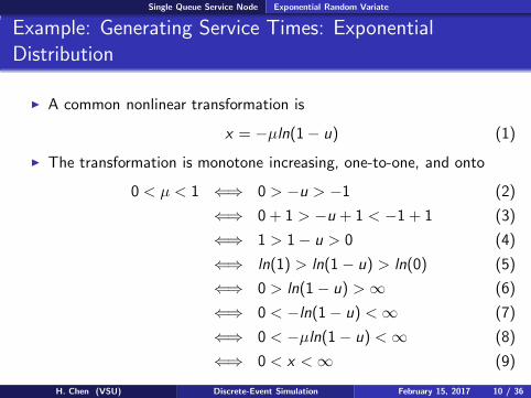
◮ A common nonlinear transformation is

x = −µln(1− u) (1)

◮ The transformation is monotone increasing, one-to-one, and onto

0 < µ < 1 ⇐⇒ 0 > −u > −1 (2)

⇐⇒ 0 + 1 > −u + 1 < −1 + 1 (3)

⇐⇒ 1 > 1− u > 0 (4)

⇐⇒ ln(1) > ln(1− u) > ln(0) (5)

⇐⇒ 0 > ln(1− u) > ∞ (6)

⇐⇒ 0 < −ln(1− u) < ∞ (7)

⇐⇒ 0 < −µln(1− u) < ∞ (8)

⇐⇒ 0 < x < ∞ (9)




◮ The common nonlinear transformation x = −µln(1− u) is monotoneincreasing, one-to-one, and onto

0 < µ < 1 ⇐⇒ 0 < −µln(1− u) < ∞ ⇐⇒ 0 < x < ∞ (10)

which generates Exponential(µ) random variate

0.0 1.00.0

x

µ

Figure: Exponential-variate-generation GeometryH. Chen (VSU) Discrete-Event Simulation February 15, 2017 11 / 36



◮ The common nonlinear transformation

x = −µln(1− u) (11)

generates Exponential(µ) random variate◮ Note that 0 < u < 1 and

∫ 1

0−µln(1 − u)du = −µ

∫ 1

0ln(1 − u)du (12)

= −µ

∫ 1

0−ln(1 − u)d(1 − u) = µ

∫ 1

0ln(1 − u)d(1 − u) (13)

= µ{ln(1 − u)(1 − u)|10 −

∫1

0(1 − u)dln(1 − u)} (14)

= µ{0 − (1 − u)1

1 − u(1 − u)|

10} (15)

= −µ(1 − u)1

1 − u(1 − u)|

10 = −µ(1 − u)|

10 (16)

= µ (17)

i.e., the parameter µ specifies the sample mean



Generating Exponential(µ) Random Variate

Definition 3.1.1 ANSI C Function for Exponential(µ)

double Exponential(double µ){return - µ * log(1.0 - Random());

}

where Random() generates u = Uniform(0, 1) random variate and µ is thesample mean.




In the single-server service node simulation, we use Exponential(µs) togenerate service times,

si = Exponential(µs); i = 1, 2, 3, . . . , n (18)

where µs is the sample mean of service times.



Example: Generating Interarrival Times: ExponentialDistribution

In the single-server service node simulation, we use Exponential(µa) togenerate interarrival times,

ai = ai−1 + Exponential(µa); i = 1, 2, 3, . . . , n (19)

where µa is the sample mean of interarrival times.



Example: Recap

◮ Inter-arrival times◮ Generating u = Uniform(a, b) random variate◮ Generating u = Exponential(a) random variate

◮ Service times◮ Generating u = Uniform(a, b) random variate◮ Generating u = Exponential(a) random variate


Single Queue Service Node Simulation Program

Simulation Program ssq2

◮ Program ssq2 is an extension of ssq1◮ Interarrival times are drawn from Exponential(2.0)◮ Service times are drawn from Uniform(1.0, 2.0)

◮ The program generates job-averaged and time-averaged statistics◮ r : average interarrival time◮ w : average wait◮ d : average delay◮ s: average service time◮ l : average # in the node◮ q: average # in the queue◮ x: server utilization



Exercise L4-1

In this exercise, you are required to complete the following tasks,

◮ Develop ssq2 by revising ssq1 program.

◮ Compile and run the ssq2 program.

◮ When writing the program, meet the following,◮ Interarrival times are drawn from Uniform(0.0, 6.0)◮ Service times are drawn from Exponential(2.0)

◮ Submission: the source code of ssq2, the results of the program, andevidence that your program appears to be correct.



Example 3.1.3: Theoretical Result from Analytic Model

◮ The theoretical averages for a single-server service node usingExponential(2.0) inter-arrivals and Uniform(1.0, 2.0) service times are(Gross and Harris, 1985),

r w d s l q x2.00 3.83 2.33 1.50 1.92 1.17 0.75

◮ Although the server is busy only 75% of the time, on average thereare approximately two jobs in the service node

◮ A job can expect to spend more time in the queue than in service

◮ To achieve these averages, many jobs must pass through node



Example 3.1.3: Results from Simulation Program ssq2

◮ The accumulated average wait was printed every 20 jobs

0 100 200 300 400 500 600 700 800 900 10002

3

4

5

6

7

8

9

Number of jobs (n)

Aver

age

wait

(w)

Seed: 12345

Seed: 54321

Seed: 2121212

Analytic Model

Figure: Average wait times

◮ The convergence of w is slow, erratic, and dependent on the initialseed



Use of Program ssq2

◮ The program can be used to study the steady-state behavior◮ Will the statistics converge independent of the initial seed?◮ How many jobs does it take to achieve steady-state behavior?

◮ It can be used to study the transient behavior◮ Fix the number of jobs processed and replicate the program with the

initial state fixed◮ Each replication uses a different initial rng seed



Exericse L4-2

You are required to reproduce the figure in slide 20. You may take stepsbelow (using the C/C++ program as an example),

◮ Convert the main function int main(void) to function voidSimulateOnce(long seed, long last).

◮ seed: seed of RNG◮ last: the number of jobs to process

◮ Add the main function in which you call SimulateOnce with seed andlast in a loop with last as the loop variable to simulate with thenumber of jobs as 20, 40, . . . , 1000.

◮ Format the output in the “CSV” format.

◮ Run the program and graph the results.

◮ Submission: program source code, running results, and graph.


Single Queue Service Node Geometric Random Variate

Geometric Random Variables

◮ The Geometric(p) random variate is the discrete analog to acontinuous Exponential(µ) random variateLet x = Exponential(µ) = µln(1− µ), y = ⌊x⌋, and p = Pr(y 6= 0)

y = ⌊x⌋ 6= 0 ⇐⇒ x ≥ 1 (20)

⇐⇒ µln(1− µ) ≥ 1 (21)

⇐⇒ ln(1− µ) ≤ −1/µ (22)

⇐⇒ 1− µ ≤ e−1/µ (23)

Since 1− µ is also Uniform(0.0, 1.0) and p = Pr(y 6= 0) = e−1/µ

Finally, since µ = −1/ln(p), y = ⌊ln(1− µ)/ln(p)⌋


Single Queue Service Node Geometric Random Variate

Generating Geometric(p) Random Variates

Definition 3.1.2 ANSI C Function for Geometric(p)

long Geometric(double p) use 0.0 < p < 1.0{return (long)(log(1.0 - Random()) / log(p));

}

◮ Random() generates u = Uniform(0, 1) random variate.

◮ The mean of a Geometric(p) random variate is p/(1− p)◮ If p is close to zero then the mean will be close to zero◮ If p is close to one, then the mean will be large


Single Queue Service Node Composite Service Model

Example 3.1.4: Composite Service Model

Now consider a composite service model

◮ Assume that jobs arrive at random with a steady-state arrival rate of0.5 jobs per minute

◮ Assume that Job service times are composite with two components◮ The number of service tasks is 1 + Geometric(0.9)◮ The time (in minutes) per task is Uniform(0.1, 0.2)



Example 3.1.4: Composite Service Model

ANSI C Function for the Composite Service Model

double GetService(void){long k;double sum = 0.0;long tasks = 1 + Geometric(0.9);for (k = 0; k < tasks; k++)sum += Uniform(0.1, 0.2);

return (sum);}



Example 3.1.4: Composite Service Model: Analytic Model

◮ The theoretical steady-state statistics for this model are

r w d s l q x2.00 5.77 4.27 1.50 2.89 2.14 0.75

◮ The arrival rate, service rate, and utilization are identical to Example3.1.3 (See slide 19)

◮ The other four statistics are significantly larger

◮ Performance measures are sensitive to the choice of service timedistribution


Simple Inventory System

Simple Inventory System: Example 3.1.5

◮ Program sis2 has randomly generated demands using anEquilikely(a, b) random variate

◮ Using random data, we can study transient and steady-state behaviors

◮ If (a, b) = (10, 50) and (s,S) = (20, 80), then the approximatesteady-state statistics are

d o u l+

l−

30.00 30.00 0.39 42.86 0.26



Exercise L4-3

In this exercise, you are required to complete the following tasks,

◮ Compile and run the sis2 program. Document the results.

◮ Make a copy of the sis2 program, revise it to meet the following,◮ The demand is drawn from Geometric(0.967742)

and then compile and run the program.

◮ Submit your work including both version of the sis2 program and theresults of both runs in Blackboard



Effects of Number of Time Intervals and Seed of RNG

◮ The average inventory level l = l+− l approaches steady state after

several hundred time intervals

0 50 100 150 20036

38

40

42

44

46

48

50

52

54

Number of Time Intervals (n)

Ave

rage

Inve

nto

ry(l

)

Seed: 12345

Seed: 54321

Seed: 2121212

Analytic Model

Figure: Number of Time Intervals (n)

◮ Convergence is slow, erratic, and dependent on the initial seed



Exercise L4-4

You are required to reproduce the figure in slide 30. You maytake steps below (using the Java program as an example),

◮ Convert the main function public static void main(String[] args) tofunction public static void SimulateOnce(long seed, long stop).

◮ seed: seed of RNG; stop: the number of intervals to process◮ Format the output in the “CSV” format

◮ Add the public static void main(String[] args function in which youcall SimulateOnce with seed and stop in a loop with stop as the loopvariable to simulate with the number of intervals as 5, 10, 15, . . .,200.

◮ Run the program and graph the results

◮ Submission: program source code, results, and graph.



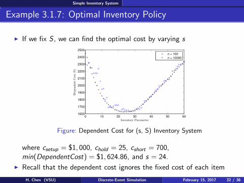
Example 3.1.7: Optimal Inventory Policy

◮ If we fix S , we can find the optimal cost by varying s

0 10 20 30 40 50 601600

1700

1800

1900

2000

2100

2200

2300

2400

2500

Inventory Parameter

Dep

enden

tC

ost

($)

n = 100

n = 10000

Figure: Dependent Cost for (s, S) Inventory System

where csetup = $1, 000, chold = 25, cshort = 700,min(DependentCost) = $1, 624.86, and s = 24.

◮ Recall that the dependent cost ignores the fixed cost of each item



Example 3.1.7: Discussion

◮ Using a fixed initial seed guarantees the exact same demand sequence◮ Any changes to the system are caused solely by the change of s

◮ A steady state study of this system is unreasonable◮ All parameters would have to remain fixed for many years◮ When n = 100 we simulate approximately 2 years◮ When n = 10000 we simulate approximately 192 years



Statistical Considerations

◮ Example 3.1.7 illustrates two consideration◮ Variance reduction◮ Robust estimation

◮ With Variance Reduction, we eliminate all sources of variance exceptone

◮ Transient behavior will always have some inherent uncertainty◮ We kept the same initial seed and changed only s

◮ Robust Estimation occurs when a data point that is not sensitive tosmall changes in assumptions

◮ Values of s close to 23 have essentially the same cost◮ Would the cost be more sensitive to changes in S or other assumed

values?



Exercise L4-5

You are required to reproduce the figure in slide 32.Hints (using the Java program as an example):

◮ Revisepublic static void SimulateOnce(long seed, long stop)

throws IOException { ......

to

public static void SimulateOnce(long seed, long stop, int slower)

throws IOException { ......

where slower is s is (s,S) in the inventory system.

◮ In the main method/function, call the SimulateOnce method/function withstop = 100 and stop = 10000, respectively in two loops whose loop variablechanges from slower = 0 to slower = 60 with increment 1.

◮ Let csetup = $1, 000, chold = 25, and cshort = 700. Compute the dependent cost inan Excel workbook. Graph the cost versus s for the two stop values.

Cdependent = csetupu + chold l++ cshort l

−

◮ Submission: both the program and the Excel workbook.



Summary

◮ Discrete-Event Simulations: random variate vs. trace

◮ Revisited SSQ

◮ Revisited SIS

◮ Variance reduction and robust estimation


Documents

Discrete-Event Simulation Lawrence M. Leemis and Stephen K