Embed Size (px)
Citation preview

DOI 10.4171/JEMS/331
J. Eur. Math. Soc. 14, 1209–1244 c© European Mathematical Society 2012
David Cimasoni
Discrete Dirac operators on Riemann surfacesand Kasteleyn matrices
Received April 19, 2010
Abstract. Let 6 be a flat surface of genus g with cone type singularities. Given a bipartite graph0 isoradially embedded in 6, we define discrete analogs of the 22g Dirac operators on 6. Thesediscrete objects are then shown to converge to the continuous ones, in some appropriate sense.Finally, we obtain necessary and sufficient conditions on the pair 0 ⊂ 6 for these discrete Diracoperators to be Kasteleyn matrices of the graph 0. As a consequence, if these conditions are met,the partition function of the dimer model on 0 can be explicitly written as an alternating sum of thedeterminants of these 22g discrete Dirac operators.
Keywords. Perfect matching, dimer model, discrete complex analysis, isoradial graph, Dirac op-erator, Kasteleyn matrices
1. Introduction
A dimer covering, or perfect matching, on a graph 0 is a collection of edges with theproperty that each vertex is adjacent to exactly one of these edges. Assigning weights tothe edges of 0 allows one to define a probability measure on the set of dimer coverings,and the corresponding model is called the dimer model on 0.
Dimer models are among the most studied in statistical mechanics. One of their re-markable properties is that the partition function of a dimer model on a graph 0 canbe written as a linear combination of 22g Pfaffians (determinants in the case of bipar-tite graphs), where g is the genus of an orientable surface 6 in which 0 embeds. These22g matrices, called Kasteleyn matrices, are skew-symmetric matrices determined by 22g
orientations of the edges of 0 ⊂ 6, called Kasteleyn orientations. P. W. Kasteleyn him-self proved this Pfaffian formula in the planar case [12, 13] together with the case of asquare lattice embedded in the torus, and stated the general fact [14]. A complete combi-natorial proof of this statement was first obtained much later by Gallucio–Loebl [10] andindependently by Tesler [18], who extended it to non-orientable surfaces.
In [5], we studied an explicit correspondance (first suggested by Kuperberg [16]) re-lating spin structures on 6 and Kasteleyn orientations on 0 ⊂ 6. We also used the iden-
D. Cimasoni: Section de mathematiques, Universite de Geneve, 2-4 rue du Lievre, 1211 Geneve 4,Suisse; e-mail: [email protected]
Mathematics Subject Classification (2010): 82B20, 57M15, 52C99
1210 David Cimasoni
tification of spin structures with quadratic forms to give a geometric proof of the Pfaffianformula, together with a geometric interpretation of its coefficients.
The partition function of free fermions on a closed Riemann surface 6 of genus gis also a linear combination of 22g determinants of Dirac operators, each term corre-sponding to a spin structure on 6 [1]. Assuming that dimer models are discrete analogsof free fermions, one expects—in addition to the known relation between Kasteleynorientations and spin structures—a relation between the Kasteleyn matrix for a givenKasteleyn orientation and the Dirac operator associated to the corresponding spin struc-ture.
This is well understood in the planar case with the work of Kenyon [15]. For anybipartite planar graph 0 satisfying some geometric condition known as isoradiality (seebelow), he defined a discrete version of the Dirac operator which turns out to be closelyrelated to a Kasteleyn matrix of 0. In particular, its determinant is equal to the par-tition function of the dimer model on 0 with critical weights. In the genus one case,the following observation was made by Ferdinand [9] as early as 1967: For the M × Nsquare lattice on the torus with horizontal weight x and vertical weight y, the determi-nants of the four Kasteleyn matrices behave asymptotically, in the M,N → ∞ limitwith fixed ratio M/N , as a common bulk term times the four Jacobi theta functionsθk(0|τ), where τ = iMx
Ny. This reproduces exactly the dependance of the determinant of
the Dirac operators on the different spin structures observed by Alvarez-Gaume, Mooreand Vafa [1].
The higher genus case remains somewhat mysterious. The only results available arenumerical evidences, for one specific example of a square lattice embedded in a genustwo surface, that the determinants of the 16 Kasteleyn matrices have a dependance thatcan be expressed in terms of genus two theta functions [6].
In short, it is fair to say that relatively little is understood of the expected relationbetween Kasteleyn matrices and Dirac operators on surfaces of genus g ≥ 2. With thispaper, we aim at filling this gap. Here is a summary of our results.
We start in Section 2 by defining a discrete analog of the ∂ operator on functions on aRiemann surface 6. Because there is no “canonical” such discretization, some geometricconditions may be naturally imposed on the pair 0 ⊂ 6. Following Duffin [7], Mer-cat [17], Kenyon [15] and many others, and for reasons that will become apparent alongthe way, we work with bipartite isoradial graphs. More precisely, we encode the complexstructure on 6 by a flat metric with cone type singularities supported at S ⊂ 6, and con-sider locally finite graphs 0 ⊂ 6 with bipartite structure V (0) = B tW satisfying thefollowing conditions:
(i) Each edge of 0 is a straight line (with respect to the flat metric on 6), and for somepositive δ, each face f of 0 ⊂ 6 contains an element xf at distance δ from everyvertex of f .
(ii) A singularity of 6 is either a black vertex of 0, or a vertex xf of the dual graph 0∗.
For such a pair 0 ⊂ 6, we introduce a discrete ∂ operator defined on CB , and callf ∈ CB discrete holomorphic if ∂f = 0. (See Definition 2.1.) This operator has somenatural properties (Proposition 2.2) and extends previous constructions of Mercat [17],

Discrete Dirac operators and Kasteleyn matrices 1211
Kenyon [15] and Dynnikov–Novikov [8]. Note that these authors impose strong condi-tions on 0 in order for ∂ to be defined: 0 needs to be the double of a graph in [17] (andtherefore does not admit any perfect matching in higher genus cases, see Remark 2.3), itneeds to be planar in [15], while only the triangular (or dually, the hexagonal) lattice isconsidered in [8]. On the other hand, our discrete ∂ operator imposes essentially no com-binatorial restriction on 0: any locally finite bipartite graph such that each white vertexhas degree at least three can be isoradially embedded in an orientable flat surface 6 withconical singularities S ⊂ V (0∗) ∪ B (Proposition 2.4). This section is concluded witha convergence theorem: if a sequence of discrete holomorphic functions converges to afunction f : 6 → C in the appropriate sense, then f is holomorphic. (See Theorem 2.5for the precise statement.)
In Section 3, we twist the discrete ∂ operator on 0 ⊂ 6 by discrete spin structures λto obtain 22g discrete Dirac operators
Dλ : CB → CW ,
provided each cone angle of 6 is a multiple of 2π (Definition 3.9). The convergencetheorem then takes the following form: let λn be a sequence of discrete spin structures on6 discretizing a fixed spin structure L. If a sequence ψn of discrete holomorphic spinors(that is, Dλnψn = 0) converges to a section ψ of the line bundle L → 6, then ψ is aholomorphic spinor. (See Theorem 3.12.)
Section 4 contains the core of this paper. First, we extend the Kasteleyn formalismfrom {±1}-valued flat cochains on 0 ⊂ 6 (that is Kasteleyn orientations) to G-valuedones for any subgroupG of C∗. We believe that the resulting existence statement (Propo-sition 4.2) and generalized Pfaffian formula (Theorem 4.3 and Corollary 4.4) are of inde-pendent interest. We use them to prove our main result:
Theorem. Let 6 be a compact oriented flat surface of genus g with conical singularitiessupported at S and cone angles multiples of 2π . Fix a graph 0 with bipartite structureV (0) = B t W , isoradially embedded in 6 so that S ⊂ B ∪ V (0∗). For an edge e of0, let ν(e) denote the length of the dual edge. Finally, let Dλ : CB → CW denote thediscrete Dirac operator associated to the discrete spin structure λ.
There exist 22g non-equivalent discrete spin structures such that the correspond-ing discrete Dirac operators {Dλ}λ give 22g non-equivalent Kasteleyn matrices of theweighted graph (0, ν), if and only if the following conditions hold:
(i) each conical singularity in V (0∗) has angle an odd multiple of 2π ;(ii) for some (or equivalently, for any) choice of oriented simple closed curves {Cj } in 0
representing a basis of H1(6;Z),∑b∈B∩Cj
αb(Cj )−∑
w∈W∩Cj
αw(Cj )
is a multiple of 2π for all j , where αv(C) denotes the angle made by the orientedcurve C at the vertex v as illustrated below.

1212 David Cimasoni
v
αv(C)C
As a consequence, given any graph 0 ⊂ 6 satisfying the conditions above, the partitionfunction for the dimer model on (0, ν) is given by
Z(0, ν) =12g
∣∣∣ ∑λ∈S(6)
(−1)Arf(λ) det(Dλ)∣∣∣,
where Arf(λ) ∈ Z2 denotes the Arf invariant of the spin structure λ (Theorems 4.9 and4.11). Our final result, Theorem 4.14, states that the Dirac operators on any closed Rie-mann surface can be approximated by Kasteleyn matrices. More precisely, for any closedRiemann surface of positive genus, there exist a flat surface 6 with cone type singulari-ties inducing this complex structure, and an isoradially embedded bipartite graph 0 ⊂ 6,with arbitrarily small radius, satisfying all the hypothesis and conditions of the theoremdisplayed above.
2. The discrete ∂ operator on Riemann surfaces
The aim of this section is to introduce a discrete analog of the ∂ operator on functions ona Riemann surface, extending works of Duffin [7], Mercat [17] and Kenyon [15]. As thisdefinition requires a substantial amount of notation and terminology, we shall proceedleisurely, starting by recalling in Subsection 2.1 the main properties of flat surfaces withconical singularities. We then give in Subsection 2.2 discrete analogs of all the geomet-ric objects involved in the definition of ∂ (see Table 1). This will lead up in Subsection2.3 to the (by then, quite natural) definition of the discrete operator. The section is con-cluded with a convergence theorem (Theorem 2.5 in Subsection 2.4), justifying furtherour definition.
2.1. Flat surfaces
Our discrete ∂ operator will be defined for graphs embedded in so-called flat surfaces withconical singularities. Since these objects are ubiquitous in the present paper, we devotethis first subsection to their main properties, referring to [19] for further details.
Given a positive real number θ , the space
Cθ = {(r, t) | r ≥ 0, t ∈ R/θZ}/(0, t) ∼ (0, t ′)
endowed with the metric ds2= dr2
+ r2dt2 is called the standard cone of angle θ . Notethat the cone without its tip is locally isometric to the Euclidean plane. Let 6 be a surfacewith a discrete subset S. A flat metric on 6 with conical singularities of angles {θx}x∈Ssupported at S is an atlas {φx : Ux → U ′x ⊂ Cθx }x∈S , where Ux is an open neighborhoodof x ∈ S, φx maps x to the tip of the cone Cθx , and the transition maps are Euclideanisometries.
Discrete Dirac operators and Kasteleyn matrices 1213
This seemingly technical definition should not hide the fact that these objects areextremely natural: any such flat surface can be obtained by gluing polygons embeddedin R2 along pairs of sides of equal length. For example, a rectangle with opposite sidesidentified will define a flat torus with no singularity. On the other hand, a regular 4g-gonwith opposite sides identified gives a flat surface of genus g with a single singularity ofangle 2π(2g − 1). In general, the topology of the surface is related to the cone anglesby the following Gauss–Bonnet formula: if 6 is a closed flat surface with cone angles{θx}x∈S , then ∑
x∈S
(2π − θx) = 2πχ(6).
For the purpose of this paper, the most important property of flat metrics is that theyencode complex structures on oriented surfaces. Indeed, the conformal structure on 6 \Sgiven by a flat metric extends to the whole oriented surface, defining a complex structureon 6. Furthermore, let 6 be a closed oriented surface, S ⊂ 6 a discrete subset, and{θx}x∈S a set of positive numbers satisfying the Gauss–Bonnet formula. Then, for eachcomplex structure on6, there exists a flat metric on6 with conical singularities of angles{θx}x∈S supported at S inducing this complex structure.
For example, any complex structure on the torus can be realized by a flat surfacewith no singularity: simply consider the parallelogram in the complex plane spanned bythe pair of periods of the torus, and identify the opposite sides. Similarly, deforming theregular octagon in such a way that the sides are organized into pairs of equal length allowsto realize any complex structure on the genus two surface.
2.2. Some discrete geometry
Let us begin by briefly recalling the definition of the ∂ and ∂ operators on a Riemannsurface 6. (This will also fix some notation). The complex structure J on 6 induces adecomposition of the complexified tangent bundle T6C into T6+⊕T6−, and thereforea decomposition of complex-valued vector fields C∞(T 6C) = C∞(T 6+)⊕C∞(T 6−).The elements of C∞(T 6+) (resp. C∞(T 6−)) are the vector fields for which the actionof J is given by multiplication by i (resp. −i). Similarly, the complex cotangent bundlesplits, resulting in a decomposition of the complex-valued 1-forms on 6:
�1(6,C) = C∞(T ∗6C) = C∞(T ∗6+)⊕ C∞(T ∗6−) = �1,0(6)⊕�0,1(6).
Note that the forms of type (1, 0) (resp. (0, 1)) are the 1-forms ϕ such that for anyvector field V , ϕ(J (V )) is equal to iϕ(V ) (resp. −iϕ(V )). Finally, the exterior deriva-tive d : C∞(6) → �1(6) induces a C-linear map dC : C∞(6,C) → �1(6,C) =�1,0(6) ⊕ �0,1(6), whose composition with the natural projections defines the Dol-beault operators ∂ : C∞(6,C)→ �1,0(6) and ∂ : C∞(6,C)→ �0,1(6). Recall that afunction f ∈ C∞(6,C) is holomorphic if and only if ∂f is zero.
We are now ready to start our discretization procedure. First and foremost, a Riemannsurface6 is a surface. To encode the topology of6, fix a locally finite graph 0 ⊂ 6 withvertex set V (0) and edge setE(0), such that6\0 consists of disjoint open discs. In other
1214 David Cimasoni
words, 0 is the 1-skeleton of a cellular decomposition of 6. For notational simplicity, weshall assume throughout this section that 0 has neither multiple edges, nor valency onevertices. (Note however that all our results hold in the general case as well.)
As explained in the previous subsection, a standard and beautiful way to encode acomplex structure on an oriented surface6 is to endow the surface with a flat metric withconical singularities. Note that any point in 6 \ S has a well-defined tangent space. Inparticular, the space X(6) of vector fields on 6 can be naively discretized by X(D), thespace of vector fields along some discrete subset D ⊂ 6 \ S.
Next, we wish to encode in the graph 0 the decomposition of X(6)C = C∞(T 6C)induced by the almost complex structure. A convenient way to do so is to consider adecomposition V (0) = B t W of the vertices of 0 into, say, black and white vertices,together with a perfect matching M on 0 pairing each black vertex b ∈ B with a whiteone w ∈ W and vice versa. Any perfect matching will do the job, provided 0 is bipartite,that is, no edge of 0 links two vertices of the same color. Hence, when the surface 6 isendowed with an almost complex structure, it is natural to consider a bipartite graph 0 ⊂6 together with a perfect matching M on it. The discrete analog of the decompositionC∞(T 6C) = C∞(T 6+) ⊕ C∞(T 6−) is then given by X(DM)
C= X(B) ⊕ X(W),
whereDM ⊂ 6 denotes the discrete set consisting of the middle point of each edge inM .The complex structure on X(B) (resp. X(W)) is such that multiplication by i correspondsto the 90 degrees rotation of the tangent vectors in the positive (resp. negative) direction,which we will represent in our figures as counterclockwise (resp. clockwise).
In the same way, �1,0(6) will be encoded by the space �1(B) :=∏b∈B X(b)∗ and
�0,1(6) by�1(W) :=∏w∈W X(w)∗, where X(v)∗ denotes the dual to the 1-dimensional
Table 1. Discretization dictionary, part 1
The geometric object The discrete analog
a surface 6 a graph 0 ⊂ 6 inducing a cellular decompositionof 6
a conformal structure on 6 a flat metric on 6 with conical singularities S ⊂ 6
the space X(6) of vector fields on 6 the space X(D) of vector fields along some discretesubset D ⊂ 6
the decomposition C∞(T 6C) =C∞(T 6+)⊕ C∞(T 6−) induced by
an almost complex structure on 6
a bipartite structure V (0) = B tW together with aperfect matching M on the graph 0, inducing a
decomposition X(DM )C= X(B)⊕ X(W)
the space �1,0(6) of (1, 0)-formson 6
�1(B) =∏b∈B X(b)∗
the space �0,1(6) of (0, 1)-formson 6
�1(W) =∏w∈W X(w)∗
the space C∞(6,C) of complexfunctions on 6
CB ' CW , identified via M
∫∫P ∂F dx dy = −
i2∫∂P F dz the definition of the discrete ∂ operator
∂ : CB → �1(W)
Discrete Dirac operators and Kasteleyn matrices 1215
complex vector space X(v) of tangent vectors at the vertex v ∈ V (0). Finally, the spaceC∞(6,C) can be discretized both by CB and by CW , which are identified via the perfectmatching M .
Table 1 summarizes our notation and the dictionary between the geometric and dis-crete objects considered in this subsection. (The last entry will be explained shortly.)
2.3. The discrete ∂ operator
Let 0 be a bipartite graph embedded in a flat surface 6 with conical singularities sup-ported at S. According to the discussion above, the operator ∂ : C∞(6,C) → �0,1(6)
should discretize to a C-linear map
∂ : CB → �1(W) =∏w∈W
X(w)∗.
These spaces make sense as soon as no white vertex is a singularity, so let us only assumeS ⊂ 6 \W for now.
Following the terminology of Kenyon [15], we shall say that 0 is isoradially embed-ded in 6 if each edge of 0 is a straight line, and if for some δ > 0, each face f of 0 ⊂ 6contains an element xf such that d(xf , v) = δ for all vertices v of ∂f . We shall further-more assume that a singularity of 6 is either a black vertex b of 0, or a vertex xf of thedual graph 0∗, that is, S ⊂ V (0∗) ∪ B.
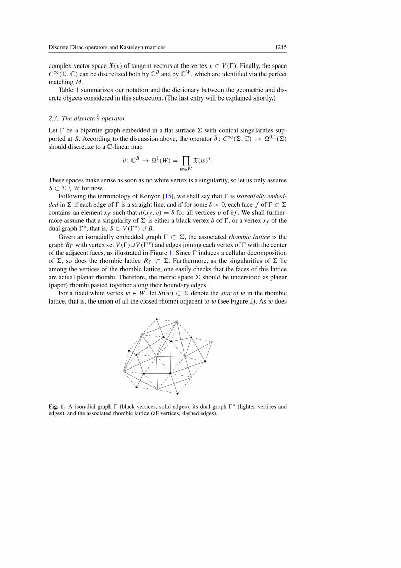
Given an isoradially embedded graph 0 ⊂ 6, the associated rhombic lattice is thegraphR0 with vertex set V (0)∪V (0∗) and edges joining each vertex of 0 with the centerof the adjacent faces, as illustrated in Figure 1. Since 0 induces a cellular decompositionof 6, so does the rhombic lattice R0 ⊂ 6. Furthermore, as the singularities of 6 lieamong the vertices of the rhombic lattice, one easily checks that the faces of this latticeare actual planar rhombi. Therefore, the metric space 6 should be understood as planar(paper) rhombi pasted together along their boundary edges.
For a fixed white vertex w ∈ W , let St(w) ⊂ 6 denote the star of w in the rhombiclattice, that is, the union of all the closed rhombi adjacent to w (see Figure 2). As w does
Fig. 1. A isoradial graph 0 (black vertices, solid edges), its dual graph 0∗ (lighter vertices andedges), and the associated rhombic lattice (all vertices, dashed edges).
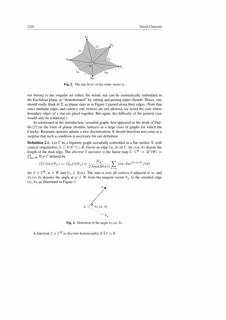
1216 David Cimasoni
b1
b2
b3
b4
bm
x1
x2x3
x4 xm
w
Fig. 2. The star St(w) of the white vertex w.
not belong to the singular set either, the whole star can be isometrically embedded inthe Euclidean plane, as “demonstrated” by cutting and pasting paper rhombi. Hence, oneshould really think of 6 as planar stars as in Figure 2 pasted along their edges. (Note thatsince multiple edges and valency one vertices are not allowed, we avoid the case whereboundary edges of a star are glued together. But again, the difficulty of the general casewould only be notational.)
As mentioned in the introduction, isoradial graphs first appeared in the work of Duf-fin [7] (in the form of planar rhombic lattices) as a large class of graphs for which theCauchy–Riemann operator admits a nice discretization. It should therefore not come as asurprise that such a condition is necessary for our definition.
Definition 2.1. Let 0 be a bipartite graph isoradially embedded in a flat surface 6 withconical singularities S ⊂ V (0∗) ∪ B. Given an edge (w, b) of 0, let ν(w, b) denote thelength of the dual edge. The discrete ∂ operator is the linear map ∂ : CB → �1(W) =∏w∈W X(w)∗ defined by
(∂f )(w)(Vw) =: (∂wf )(Vw) =|Vw|
2 Area(St(w))
∑b∼w
ν(w, b)eiϑV (w,b)f (b)
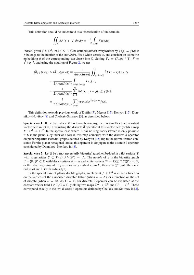
for f ∈ CB , w ∈ W and Vw ∈ X(w). The sum is over all vertices b adjacent to w, andϑV (w, b) denotes the angle at w ∈ W from the tangent vector Vw to the oriented edge(w, b), as illustrated in Figure 3.
w
b
ϑV (w, b)
Vw
Fig. 3. Definition of the angle ϑV (w, b).
A function f ∈ CB is discrete holomorphic if ∂f = 0.
Discrete Dirac operators and Kasteleyn matrices 1217
This definition should be understood as a discretization of the formula∫∫P
∂F (x + iy) dx dy = −i
2
∫∂P
F(z) dz.
Indeed, given f ∈ CB , let f : 6→ C be defined (almost everywhere) by f (p) = f (b) ifp belongs to the interior of the star St(b). Fix a white vertex w, and consider an isometricembedding φ of the corresponding star St(w) into C. Setting Vw = (Twφ)
−1(1), F =f ◦ φ−1, and using the notation of Figure 2, we get
(∂wf )(Vw) ≈ (∂F )(φ(w)) ≈1
Area(St(w))
∫∫φ(St(w))
∂F (x + iy) dx dy
=−i
2 Area(St(w))
∫φ(∂St(w))
F(z) dz
=1
2 Area(St(w))
m∑j=1
i(φ(xj−1)− φ(xj ))f (bj )
=1
2 Area(St(w))
∑b∼w
ν(w, b)eiϑV (w,b)f (b).
This definition extends previous work of Duffin [7], Mercat [17], Kenyon [15], Dyn-nikov–Novikov [8] and Chelkak–Smirnov [3], as described below.
Special case 1. If the flat surface6 has trivial holonomy, there is a well-defined constantvector field in X(W). Evaluating the discrete ∂ operator at this vector field yields a mapK : CB → CW . In the special case where 6 has no singularity (which is only possibleif 6 is the plane, a cylinder or a torus), this map coincides with the discrete ∂ operatoron planar bipartite isoradial graphs defined by Kenyon [15] (up to the normalization con-stant). For the planar hexagonal lattice, this operator is conjugate to the discrete ∂ operatorconsidered by Dynnikov–Novikov in [8].
Special case 2. Let G be a (not necessarily bipartite) graph embedded in a flat surface 6with singularities S ⊂ V (G) ∪ V (G∗) =: 3. The double of G is the bipartite graph0 = G∪G∗ ⊂ 6 with black vertices B = 3 and white verticesW = E(G)∩E(G∗) =: ♦,or the other way around. If G is isoradially embedded in 6, then so is G∗ (with the sameradius δ) and 0 (with radius δ/2).
In the special case of planar double graphs, an element f ∈ CB is either a functionon the vertices of the associated rhombic lattice (when B = 3), or a function on the setof rhombi (when B = ♦). As 6 = C, our discrete ∂ operator can be evaluated at theconstant vector field 1 ∈ TpC = C, yielding two maps C3→ C♦ and C♦
→ C3. Thesecorrespond exactly to the two discrete ∂ operators defined by Chelkak and Smirnov in [3].

1218 David Cimasoni
wx x′
y
y′Special case 3. Finally, let us consider the more general case ofdouble graphs isoradially embedded in flat surfaces with conicalsingularities, with bipartite structure B = 3. Let w ∈ W = ♦be a fixed rhombus, and let x, y, x′, y′ denote its vertices enu-merated counterclockwise, as illustrated above. Then the equality∂wf = 0 coincides with the very intuitive “discrete Cauchy–Riemann equation” studiedby Duffin [7] (in the planar case) and Mercat [17]:
f (y′)− f (y)
d(y, y′)= i
f (x′)− f (x)
d(x, x′).
Let us mention several natural properties of the discrete ∂ operator.
Proposition 2.2. The discrete ∂ operator has the following properties:
(i) If f ∈ CB is constant, then ∂f = 0.(ii) Given a fixed white vertex w, let f ∈ CB∩St(w) be the restriction of a coordinate
chart on a neighborhood of St(w). Then ∂wf = 0 .(iii) Let f ∈ CB∩St(w) be as in (ii) above. Then its complex conjugate f satisfies
(∂wf )(Vw) = |Vw|.
Proof. Let f ∈ CB be a constant function. Fix a white vertex w ∈ W and a unit tangentvector Vw ∈ X(w). Let φ : St(w) → C be an isometric embedding mapping w to theorigin and Vw to the direction of the unit vector 1 ∈ C = T0C. With the notation ofFigure 2, observe that for all j ,
ν(w, bj )eiϑV (w,bj ) = i(φ(xj )− φ(xj−1)),
as both these complex numbers have the same modulus and argument. It follows that
(∂wf )(Vw) =f (b1)i
2 Area(St(w))
m∑j=1
(φ(xj−1)− φ(xj )
)= 0,
proving the first claim. To check the second one, let φ : U → C be a coordinate chartwith St(w) ⊂ U , and let Vw ∈ X(w) be the unit tangent vector corresponding to the edge(w, xm) (recall Figure 2). By the first item above, it may be assumed that φ(w) = 0.Clearly, one can also assume that Twφ(Vw) = 1 ∈ T0C. For j = 1, . . . , m, let αj denotethe angle at w of the rhombus corresponding to the edge (w, bj ). Note that
sin(αj ) = 2 sin(αj/2) cos(αj/2) =ν(w, bj )d(w, bj )
2δ2 .
Since f (bj ) = φ(bj ) = d(w, bj )eiϑV (w,bj ), we get
2 Area(St(w))(∂wf )(Vw) =m∑j=1
ν(w, bj )eiϑV (w,bj )f (bj )

Discrete Dirac operators and Kasteleyn matrices 1219
=
m∑j=1
ν(w, bj )d(w, bj )ei2ϑV (w,bj ) = −iδ2
m∑j=1
(eiαj − e−iαj )ei(∑j−1k=1 2αk+αj )
= −iδ2m∑j=1
(e2i
∑j
k=1 αk − e2i∑j−1k=1 αk
)= 0,
using the fact that∑mk=1 αk = 2π . Finally,
(∂wf )(Vw) =|Vw|
2 Area(St(w))
m∑j=1
ν(w, bj )d(w, bj ) = |Vw|,
showing the third claim. ut
Remark 2.3. As pointed out in the special cases above, most authors have considereddiscrete ∂ operators defined on double graphs only. It is however crucial for us to considermore general graphs, for the following reason. In Section 4, we shall turn to the problemof counting perfect matchings on a (finite) bipartite graph 0 embedded in a (compact)surface 6. For such a matching to exist, one necessary condition is that the number ofblack vertices equals the number of white ones. But in the case of a double graph 0 =D(G) ⊂ 6, this condition gives
0 = |B| − |W | = |V (G)| + |F(G)| − |E(G)| = χ(6).
Hence, no double graph as above admits a perfect matching unless 6 is a torus.
On the other hand, our setting imposes almost no restriction on the combinatorial typeof the graphs considered:
Proposition 2.4. Let 0 be a locally finite bipartite graph such that each white vertex hasdegree at least three. Then 0 can be isoradially embedded in an orientable flat surface 6with conical singularities S ⊂ V (0∗) ∪ B.
Proof. For each w ∈ W , fix a cyclic ordering of the m adjacent edges (so that multipleedges are consecutive) and form the symmetric star St(w) by pasting together m rhombiof side length δ and of angle 2π/m according to this ordering. Note that the surface St(w)is endowed with an orientation given by the cyclic ordering. In case of multiple edges orblack vertices of degree 1, identify the corresponding boundary edges of St(w) accord-ingly. (This respects the orientation of the star.) For each b ∈ B, fix a cyclic ordering ofthe adjacent edges, and glue the stars St(w) along their boundary edges according to theseorderings, in the unique way compatible with the orientations of the stars. The result isan oriented flat surface 6 with conical singularities supported at S. By construction, 0 isisoradially embedded in 6 and S is contained in V (0∗) ∪ B. ut
As an example, consider the complete bipartite graphK3,3. With a naturalchoice of the cyclic orderings around the vertices, the construction aboveyields the honeycomb lattice embedded in the flat torus illustrated oppo-site. (The pairs of opposite sides of the big hexagon are identified.)

1220 David Cimasoni
To conclude this subsection, note that if S ⊂ 6 \ B, one can define the discrete ∂operator as the C-linear map ∂ : CW → �1(B) =
∏b∈B X(b)∗ given by
(∂bg)(Ub) =|Ub|
2 Area(St(b))
∑w∼b
ν(w, b)e−iϑU (w,b)g(w)
for g ∈ CW , b ∈ B and Ub ∈ X(b). Here again, the sum is over all vertices w adjacentto b, and ϑU (w, b) denotes the angle at b ∈ B from the tangent vector Ub to the orientededge (w, b). This construction generalizes the one given in [15], which corresponds tothe case with no singularity. However, the discrete ∂ operator being sufficient for ourpurposes, we shall not study ∂ in the present paper.
2.4. A convergence theorem
The aim of this subsection is to prove the following result.
Theorem 2.5. Let6 be a flat surface with conical singularities supported at S. Considera sequence 0n of bipartite graphs isoradially embedded in 6 with S ⊂ V (0∗n) ∪ Bn.Assume that the radii δn of 0n converge to 0, and that there is some η > 0 such thatall rhombi angles of all these 0n’s belong to [η, π − η]. Let fn ∈ CBn be a sequenceof discrete holomorphic functions converging to a function f : 6 → C in the followingsense: for any sequence xn ∈ Bn converging in 6, the sequence fn(xn) converges tof (limn xn) in C. Then the function f is holomorphic in 6.
Our proof will follow the same lines as the one of Mercat [17, pp. 192–195], a notableexception being the discrete Morera Theorem below (Lemma 2.8). Let us start with astraightforward generalization of [17, Lemma 2].
Lemma 2.6. Let X be a metric space. Consider a sequence of functions fn : X → Cconverging to f : X → C in the following sense: for any convergent sequence xn in X,the sequence fn(xn) converges to f (limn xn) in C. Then the function f is continuous, andis the uniform limit of fn on any compact.Proof. To show that f is continuous at an arbitrary point x ∈ X, pick a sequence xjconverging to x in X. For any j = 1, 2, . . . , the hypothesis applied to the constant se-quence xj yields the existence of an index nj such that |fnj (xj )−f (xj )| < 1/j . Let yn bethe sequence given by yn = xj if n = nj , and yn = x else. As yn converges to x, fn(yn)converges to f (x) and so does the subsequence fnj (xj ). It follows that
|f (xj )− f (x)| ≤ |f (xj )− fnj (xj )| + |fnj (xj )− f (x)|
is arbitarily small, proving the first claim.To show the second one, let us assume for contradiction that fn does not converge
uniformly on some fixed compact C ⊂ X. This would imply the existence of a convergentsequence xn in C with |fn(xn) − f (xn)| greater than some ε > 0 for all n. On the otherhand, the hypothesis together with the continuity of f at x = limn xn implies
|fn(xn)− f (xn)| ≤ |fn(xn)− f (x)| + |f (x)− f (xn)| < ε
for n large enough, a contradiction. ut

Discrete Dirac operators and Kasteleyn matrices 1221
Lemma 2.7. Let 0 be a graph isoradially embedded in the Euclidean plane, such thatall rhombi angles belong to the interval [η, π − η] for some η > 0. Then, for any vertexv of 0, and for any two elements x, x′ in the boundary ∂St(v) of the star of v,
d∂St(v)(x, x′)
|x − x′|≤
2πη sin(η/2)
.
Proof. To simplify the notation, let S stand for the star St(v) throughout this proof. Ifx and x′ belong to the same rhombus of S, then the quotient above is easily seen to bemaximal when x and x′ are at the same distance to the vertex opposite to v. In such acase, this quotient is equal to 1/sin(α/2), where α denotes the angle of this rhombus at v.Since η ≤ α ≤ π − η, it follows that
d∂S(x, x′)
|x − x′|≤
1sin(α/2)
≤1
sin(η/2)≤
2πη sin(η/2)
.
Let us now assume that x and x′ belong to adjacent edges, but distinct rhombi of S. Ifthe corresponding angles at w are equal to α and α′, then the argument above gives theinequality
d∂S(x, x′)
|x − x′|≤
1sin((α + α′)/2)
≤1
sin(η)≤
2πη sin(η/2)
.
If x and x′ lie on adjacent rhombi, but non-adjacent edges of the star, then |x − x′| isbounded below by δ sin(η), where δ denotes the length of the rhombus edges. On theother hand, d∂S(x, x′) ≤ 4δ as x and x′ belong to adjacent rhombi. Therefore, in this case
d∂S(x, x′)
|x − x′|≤
4sin(η)
≤2π
η sin(η/2).
Finally, consider the case where x and x′ do not belong to adjacent rhombi. Fix a rhombusbetween them, and let α denote its angle at v. This time, |x − x′| is bounded below by2δ sin(α/2) ≥ 2δ sin(η/2), while the distance in ∂S is bounded above by half of thelength of ∂S, that is
d∂S(x, x′) ≤
`(∂S)
2= #{rhombi in S} · δ ≤
2πδη.
This impliesd∂S(x, x
′)
|x − x′|≤
π
η sin(η/2)≤
2πη sin(η/2)
,
and concludes the proof. ut
The last lemma requires some preliminaries. As above, let 0 be a bipartite graph isora-dially embedded in a flat surface 6. Given a function f : 6 → C and a white vertex wof 0, set ∫
∂St(w)f :=
∫ b
a
f (γ (t))(φ ◦ γ )′(t) dt,

1222 David Cimasoni
where γ : [a, b] → St(w) is a parametrization of ∂St(w) and φ : St(w) ↪→ C is anisometric embedding. Obviously, the value of this integral depends on the choice of thechart φ. However, the choice of another chart would multiply the result by a modulus 1complex number. In particular, the vanishing of this integral does not depend on thatchoice, and the following statement makes sense.
Lemma 2.8 (discrete Morera Theorem). Let 0 be a bipartite graph isoradially embed-ded in a flat surface 6 with conical singularities S ⊂ V (0∗) ∪ B. Given f ∈ CB ,let f : 6 → C be the function defined by f (p) = 1
m
∑mj=1 f (bj ) if p belongs to⋂m
j=1 St(bj ). Then f is discrete holomorphic if and only if∫∂St(w) f = 0 for all w ∈ W .
Proof. Let w be a white vertex, and let φ : St(w)→ C be an isometric embedding of thecorresponding star. Fixing a unit vector Vw ∈ X(w), one can assume that Twφ maps Vwto 1 ∈ C. With the notation of Figure 2, we get the equality∫
∂St(w)f =
m∑j=1
(φ(xj )− φ(xj−1))f (bj ) = 2i Area(St(w))(∂wf )(Vw),
and the lemma follows. ut
Proof of Theorem 2.5. As in Lemma 2.8, extend fn ∈ CBn to a function fn : 6 → Cby setting fn(p) = 1
m
∑mj=1 fn(bj ) if p belongs to
⋂mj=1 St(bj ). By assumption, there
is a function f : 6 → C such that, for any sequence xn ∈ Bn converging in 6, thesequence fn(xn) converges to f (limn xn) in C. We claim that this statement remains truefor the extensions fn : 6→ C. Indeed, let us fix a sequence xn in 6 converging to x. Forall n, there exist black vertices b(1)n , . . . , b
(m)n such that xn belongs to the star St(b(j)n ) for
j = 1, . . . , m. Let bn (resp. b′n) be one of these vertices where Re fn is maximal (resp.minimal) on this set. By definition,
Re fn(b′n) ≤ Re fn(xn) ≤ Re fn(bn).
Since bn, b′n and xn all belong to the adjacent (or identical) stars St(bn) and St(b′n) whosediameter is at most 4δn, and since δn converges to zero, both sequences bn and b′n convergeto x = limn xn. By the assumption, fn(bn) and fn(b′n) both converge to f (x). By theinequalities displayed above, Re fn(xn) converges to Re f (x). The same argument showsthat Im fn(xn) converges to Im f (x), proving the claim.
Lemma 2.6 asserts that f : 6→ C is continuous and the uniform limit of fn : 6→ Con any compact. Since the singular set S ⊂ 6 is discrete and f is continuous, it is nowsufficient to check that f is holomorphic on 6 \ S. Hence, we can restrict ourselves to(simply connected) domains of a Euclidean atlas for the flat surface S ⊂ 6. In otherwords, we can assume that we are working in a simply connected planar domain U ⊂ C.Finally, by Morera’s theorem, it is enough to show that
∫γf (z) dz vanishes for any piece-
wise smooth loop γ in U .So, let γ be such a loop, let ` denote its length, and let n be a fixed index. Each time
γ meets some star St(wn), entering it at a point x and leaving it at x′, replace γ ∩ St(wn)by the path in ∂St(wn) realizing the minimal distance in ∂St(wn) between x and x′. This
Discrete Dirac operators and Kasteleyn matrices 1223
yields a new loop γn contained in St0n , the union of all rhombus edges adjacent to blackvertices of 0n. By Lemma 2.7, its length satisfies
`(γn) =∑wn∈Wn
`(γn ∩ St(wn)) ≤ M(η)∑wn∈Wn
|x − x′| ≤ M(η)`,
where M(η) stands for the uniform bound 2π/(η sin(η/2)). As the diameter of a starSt(wn) is at most 4δn, the union of all these stars meeting γ is contained in the tubularneighborhood of γ of diameter 8δn, which also contains the compact set Cn enclosed byγ and γn. Therefore, Area(Cn) ≤ 8δn`.
We shall now prove that the sequence∫γnf (z) dz converges to
∫γf (z) dz. Let us first
assume that f is of class C1. In that case, ∂f is bounded above by some constant Mon the compact set C given by the tubular neighborhood of γ of diameter 8 maxn δn. AsC contains all the Cn’s, this yields a uniform bound for ∂f on all Cn’s. By the Stokesformula and the inequality above,∣∣∣∣∫
γ
f (z) dz−
∫γn
f (z) dz
∣∣∣∣ = ∣∣∣∣∫∂Cn
f (z) dz
∣∣∣∣ = ∣∣∣∣∫∫Cn
∂f (z) dz ∧ dz
∣∣∣∣≤
∫∫Cn
|∂f (z)| dz ∧ dz ≤ 8δn`M,
proving the claim in this special case. In the general case of a continuous function f , letgk be a sequence of C1 functions on U converging uniformly to f on every compact. Bythe inequalities displayed above, we obtain∣∣∣∣∫
γ
f −
∫γn
f
∣∣∣∣ ≤ ∣∣∣∣∫γ
f −
∫γ
gk
∣∣∣∣+ ∣∣∣∣∫γ
gk −
∫γn
gk
∣∣∣∣+ ∣∣∣∣∫γn
gk −
∫γn
f
∣∣∣∣≤ ` sup
C
|f − gk| + 8δn`M +M(η)` supC
|f − gk|
is arbitrarily small, proving the claim.Recall that fn converges uniformly to f on the compact C. Therefore, for any fixed
index k, ∣∣∣∣∫γk
fn(z) dz−
∫γk
f (z) dz
∣∣∣∣ ≤ M(η)` supC
|fn − f |
is arbitarily small, so∫γkfn converges to
∫γkf .
We are finally ready to show that∫γf (z) dz is equal to zero. As St0n induces a cel-
lular decomposition of the simply connected domain U , the cycle γn ⊂ St0n is a cellularboundary, that is, γn = ∂(
∑wn
St(wn)) for some vertices wn. Since fn is discrete holo-morphic, Lemma 2.8 implies∫
γn
fn(z) dz =∑wn
∫∂St(wn)
fn(z) dz = 0.
By the three claims above,∫γ
f (z) dz = limk
∫γk
f (z) dz = limk
limn
∫γk
fn(z) dz = limn
∫γn
fn(z) dz = 0. ut
1224 David Cimasoni
3. Discrete Dirac operators on Riemann surfaces
In the previous section, we defined a discrete analog of the ∂ operator on functions on aRiemann surface6. The aim of the present section is to modify this construction, yieldingan analog of the Dirac operatorD on spinors on6. Here again, we shall start by giving inSubsection 3.1 discretizations of all the geometric objects involved in the definition of D(Table 2). The actual definition of the discrete Dirac operator is to be found in Subsec-tion 3.2, while Subsection 3.3 deals with the application of our convergence theorem tospinors (Theorem 3.12).
3.1. More discrete geometry
Let us first recall the definition of the Dirac operator on a closed Riemann surface 6, re-ferring to [2] for details. Let (ϕα : Uα → C)α be an atlas for6, and let fαβ : ϕβ(Uα∩Uβ)→ ϕα(Uα∩Uβ) denote the corresponding transition functions. Then καβ : Uα∩Uβ → C∗given by καβ(p) = f ′αβ(ϕβ(p))
−1 is a holomorphic function, that is, καβ is an elementof the Cech cochain group C1(U,O∗), where U = (Uα) and O∗ denotes the sheaf ofnon-vanishing holomorphic functions on 6. By the chain rule, it is actually a cocy-cle, so it defines an element in H 1(U,O∗). The corresponding holomorphic line bundleK ∈ H 1(6,O∗) is called the canonical bundle over 6. With the notation of Section 2,K is nothing other than the holomorphic cotangent bundle T ∗6+, while K coincideswith T ∗6−. Hence, the ∂ operator can be seen as a map ∂ : C∞(1)→ C∞(K), where 1denotes the trivial line bundle.
The set S(6) of spin structures on 6 can be defined as the set of isomorphism classesof holomorphic line bundles that are square roots of K , that is,
S(6) = {L ∈ H 1(6,O∗) | L2= K}.
This is easily seen to be an affine space over H 1(6;Z2). Note that a spin structure L isgiven by a cocycle (λαβ) ∈ Z1(U,O∗) such that λ2
αβ = καβ . Then a spinor ψ ∈ C∞(L)can be described by a family of smooth functions ψα ∈ C∞(Uα) such that ψα(p) =λαβ(p)ψβ(p) for p ∈ Uα∩Uβ . Since λαβ is holomorphic, the assignment (ψα) 7→ (∂ψα)
defines a map∂L : C∞(L)→ C∞(L⊗ K),
called the twisted ∂ operator. An element ψ ∈ C∞(L) is a holomorphic spinor if it is inthe kernel of ∂L.
Finally, the choice of a hermitian metric on 6 allows one to define an anti-linearisomorphism h : C∞(L⊗ K)→ C∞(L). The Dirac operator is the self-adjoint operatoron C∞(L)⊕ C∞(L) whose restriction to C∞(L) is given by
DL = h ◦ ∂L : C∞(L)→ C∞(L).
By abuse of language, we shall also call DL the Dirac operator.Let us now give discrete analogs of the objects described above. As explained in the
previous section, an analog of a Riemann surface is a bipartite graph 0 embedded in a flat

Discrete Dirac operators and Kasteleyn matrices 1225
surface 6 with cone type singularities supported at S, inducing a cell decomposition Xof 6. Furthermore, in order to define ∂ : CB → �1(W), we assumed that 0 is isoradiallyembedded in 6, with S contained in B ∪ V (0∗).
By definition, 60 := 6 \ S is endowed with an atlas whose transition functionsare Euclidean isometries. Therefore, the associated Cech cocycle consists of S1-valuedconstant functions. This defines an element K0 of H 1(60; S
1). Using the long exactsequence for the pair (6,60), one easily checks that K0 is the restriction of a class[κ] ∈ H 1(6; S1) = H 1(X; S1) if and only if exp(iθx) = 1 for all x ∈ S. We shalltherefore assume that all cone angles θx are positive multiples of 2π , and call such a co-cycle κ ∈ Z1(X; S1) a discrete canonical bundle over 6. Note that the cohomology classof κ is uniquely determined by the flat metric on 6 and the cellular decomposition X.Furthermore, such a cocycle κ is very easy to compute, as demonstrated by the followingremarks.
Remark 3.1. If the flat surface 6 has trivial holonomy, one can simply choose κ = 1 asdiscrete canonical bundle.
Remark 3.2. It is always possible to represent 6 as planar polygons P with bound-ary identifications. Furthermore, these polygons can be chosen so that 0 intersects ∂Ptransversally, except at possible singularities in S ∩ B. Define κ by
κ(e) =
{1 if e is contained in the interior of P ,exp(−iϑ) if e meets ∂P transversally,
where ϑ denotes the angle between the sides of ∂P ⊂ C met by the edge e. If S is con-tained in V (0∗), this defines completely a natural choice of discrete canonical bundle κ .If S ∩B is not empty, the partially defined κ above can be extended to a cocycle yieldinga discrete canonical bundle.
Example 3.3. Let P be the regular 4g-gon with boundary identification according to theword
∏g
j=1 ajbja−1j b−1
j . This defines a flat metric on the genus g orientable surface 6gwith one singularity of angle 2π(2g−1). Given a graph0 ⊂ 6g meeting ∂P transversally,the associated canonical bundle is given by κ(e) = exp(−iπ g−1
g) for edges of 0 meeting
∂P , and κ(e) = 1 for interior edges.
Finally, note that the assumption that all cone angles are multiples of 2π simplymeans that6 has trivial local holonomy. In that case, the holonomy defines an element ofHom(π1(6), S
1) = H 1(6; S1) = H 1(X; S1), and a representative of this cohomologyclass is exactly the inverse of a discrete canonical bundle. Note also that this assumptionrules out the 2-sphere from our setting.
Mimicking the continuous case, let us define a discrete spin structure on 6 as anycellular 1-cocycle λ ∈ Z1(X; S1) such that λ2
= κ . (See [5] for another notion ofdiscrete spin structure, valid for any cellular decomposition of an orientable surface.)Two discrete spin structures will be called equivalent if they are cohomologous. The setS(X) of equivalence classes of discrete spin structures on 6 is then given by
S(X) = {[λ] ∈ H 1(X; S1) | [λ]2= [κ]}.

1226 David Cimasoni
One easily checks that this set admits a freely transitive action of the abelian groupH 1(6; {±1}). In other words, and using additive notation, S(X) is an affine H 1(6;Z2)-space. Therefore, there exist (non-canonical) H 1(6;Z2)-equivariant bijections S(X)→S(6). Furthermore:
Proposition 3.4. If all cone angles of 6 are odd multiples of 2π , then there exists acanonical H 1(6;Z2)-equivariant bijection S(X)→ S(6).
Proof. Let κ ∈ Z1(X; S1) be a fixed discrete canonical bundle over 6. For each λ ∈Z1(X; S1) such that λ2
= κ , we shall now construct a vector field Vλ on6 with zeroes ofeven index. Such a vector field is well-known to define a spin structure, or equivalently—by Johnson’s theorem [11] – a quadratic form qλ on H1(6;Z2). The proof will be com-pleted with the verification that two equivalent λ’s induce identical quadratic forms, andthat the assignment [λ] 7→ qλ is H 1(6;Z2)-equivariant.
Let λ ∈ Z1(X; S1) be given by λ(e) = exp(iβλ(e)) with 0 ≤ βλ(e) < 2π , where e isan edge of X oriented from the white end to the black end, and set βλ(−e) = −βλ(e).
First, replace the cellular decomposition X of 6by X′, where each singularity b ∈ B ∩ S is re-moved as illustrated opposite. Obviously, λ induces λ′ ∈Z1(X′; S1) by setting λ′(e) = 1 for each newly creatededge e. Now, fix an arbitrary tangent vector Vλ(w) atsome white vertex w, and extend it to the 1-skeleton 0′
of X′ as follows: running along an edge e oriented from the white end to the black end,rotate the tangent vector by an angle of 2βλ(e) in the negative direction. (On the newlycreated edges, just extend the vector field without any rotation.) As λ′ is a cocycle, λ2
= κ
and each cone angle is a multiple of 2π , this gives a well-defined vector field along 0′.Extend it to the whole surface 6 by the cone construction. The resulting vector field Vλhas one zero at the center of each face ofX, and at each b ∈ B∩S. One easily checks thatsuch a zero is of even index if and only if the corresponding cone angle is an odd multipleof 2π , which we assumed.
Following [11], the quadratic form qλ : H1(6;Z2) → Z2 corresponding to Vλ isdetermined as follows: for any regular oriented simple closed curveC ⊂ 6\S, qλ([C])+1is equal to the winding number of the tangential vector field along C with respect to thevector field Vλ. For an oriented simple closed curve C ⊂ 0, we obtain the followingequality modulo 2:
qλ([C]) = 1+1
2π
(∑e⊂C
2βλ(e)+∑v∈C
(π − αv(C)))
= 1+|C|
2+
12π
(∑e⊂C
2βλ(e)−∑v∈C
αv(C)),
v
αv(C)Cwhere the first sum is over all oriented edges in the oriented curve
C, and αv(C) is the angle illustrated opposite. Obviously, equiva-lent λ’s induce the same quadratic form qλ. Finally, given two dis-crete spin structures λ1, λ2, the cohomology class of the 1-cocycle

Discrete Dirac operators and Kasteleyn matrices 1227
λ1/λ2 ∈ Z1(X; {±1}) is determined by its value on oriented simple closed curves in 0.
For such a curve C, we have
(λ1/λ2)(C) = exp(i∑e⊂C
(βλ1(e)− βλ2(e)))= exp(iπ(qλ1 − qλ2)([C])).
Therefore, the assignment [λ] 7→ qλ is H 1(6;Z2)-equivariant, which concludes theproof. ut
Remark 3.5. If the flat surface6 has trivial holonomy, then [κ] is trivial, so the set S(X)is equal to the 2g-dimensional vector space H 1(6;Z2).
Remark 3.6. Let 0 ⊂ 6 be described via planar polygons as explained in Remark 3.2,and let us assume that the singular set S is contained in V (0∗). In that case, a discretespin structure is given by
λ(e) =
{1 if e is contained in the interior of P ,exp(−iϑ/2) if e meets ∂P ,
where exp(−iϑ/2) denotes one of the square roots of the angle between the sides of∂P ⊂ C met by the edge e.
Example 3.7. For 6 as in Example 3.3 above, equivalence classes of spin structurescorrespond to the 22g choices of 2g square roots of exp(−iπ g−1
g), one for each pair of
boundary edges of P . In particular, for the flat torus, S(X) corresponds to the four possiblechoices of two square roots of the unity.
Let us now turn to spinors. Given a spin structure L ∈ S(6), the universal coveringπ : 6→ 6 induces the following pullback diagram:
E5 //
π∗p��
L
p
��6
π // 6
By the lifting property of the covering map 5 : E → L, any spinor ψ ∈ C∞(L) inducesa section ψ ∈ C∞(E) such that 5 ◦ ψ = ψ ◦ π , unique up to the action of π1(6). Since6 is contractible (recall that the 2-sphere is ruled out by the assumption on the coneangles), the line bundle E → 6 is trivial. Hence, ψ is really a complex-valued functionon 6 satisfying some π1(6)-periodicity property depending on L. This alternative pointof view on spinors leads to the following definition.
Let λ ∈ Z1(X; S1) be a discrete spin structure on 6, and let π : X → X denote thecellular map given by the universal covering of 6. Note that the bipartite structure on 0lifts to a bipartite structure V (0) = B ∪ W on 0 = π−1(0). The space C(λ) of discretespinors is the set of all ψ ∈ CB such that, for any b, b′ ∈ B with π(b) = π(b′),
ψ(b′) = λ(π(γb,b′))ψ(b),
1228 David Cimasoni
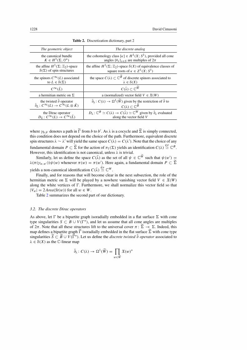
Table 2. Discretization dictionary, part 2
The geometric object The discrete analog
the canonical bundleK ∈ H 1(6,O∗)
the cohomology class [κ] ∈ H 1(X; S1), provided all coneangles {θx}x∈S are multiples of 2π
the affine H 1(6;Z2)-spaceS(6) of spin structures
the affine H 1(6;Z2)-space S(X) of equivalence classes ofsquare roots of κ ∈ Z1(X; S1)
the spinors C∞(L) associatedto L ∈ S(6)
the space C(λ) ⊂ CB of discrete spinors associated toλ ∈ S(X)
C∞(L) C(λ) ⊂ CW
a hermitian metric on 6 a (normalized) vector field V ∈ X(W)
the twisted ∂ operator∂L : C∞(L)→ C∞(L⊗ K)
∂λ : C(λ)→ �1(W ) given by the restriction of ∂ toC(λ) ⊂ CB
the Dirac operatorDL : C∞(L)→ C∞(L)
Dλ : CB ' C(λ)→ C(λ) ' CW given by ∂λ evaluatedalong the vector field V
where γb,b′ denotes a path in 0 from b to b′. As λ is a cocycle and 6 is simply connected,this condition does not depend on the choice of the path. Furthermore, equivalent discretespin structures λ ∼ λ′ will yield the same spaceC(λ) = C(λ′). Note that the choice of any
fundamental domain P ⊂ 6 for the action of π1(6) yields an identification C(λ)ϕP' CB .
However, this identification is not canonical, unless λ is trivial.Similarly, let us define the space C(λ) as the set of all ψ ∈ CW such that ψ(w′) =
λ(π(γw,w′))ψ(w) whenever π(w) = π(w′). Here again, a fundamental domain P ⊂ 6
yields a non-canonical identification C(λ)ϕP' CW .
Finally, and for reasons that will become clear in the next subsection, the role of thehermitian metric on 6 will be played by a nowhere vanishing vector field V ∈ X(W)along the white vertices of 0. Furthermore, we shall normalize this vector field so that|Vw| = 2 Area(St(w)) for all w ∈ W .
Table 2 summarizes the second part of our dictionary.
3.2. The discrete Dirac operators
As above, let 0 be a bipartite graph isoradially embedded in a flat surface 6 with conetype singularities S ⊂ B ∪ V (0∗), and let us assume that all cone angles are multiplesof 2π . Note that all these structures lift to the universal cover π : 6 → 6. Indeed, thismap defines a bipartite graph 0 isoradially embedded in the flat surface 6 with cone typesingularities S ⊂ B ∪ V (0∗). Let us define the discrete twisted ∂ operator associated toλ ∈ S(X) as the C-linear map
∂λ : C(λ)→ �1(W ) =∏w∈W
X(w)∗

Discrete Dirac operators and Kasteleyn matrices 1229
defined by the restriction of the discrete ∂ operator ∂ : CB → �1(W ) to C(λ) ⊂ CB .We need a map �1(W )→ CW discretizing the anti-linear isomorphism C∞(L⊗ K)
→ C∞(L) induced by a hermitian metric. A discrete hermitian metric, that is, a nor-malized vector field V ∈ X(W) induces a very natural such map, namely the evalua-tion at V ∈ X(W ), the lift of V to W . Putting all the pieces together yields the mapD′λ : C(λ)→ CW given by
(D′λψ)(w) =∑b∼w
ν(w, b)eiϑV (w,b)ψ(b),
with the notation of Subsection 2.3. One easily checks that the image of D′λ is containedin C(λ), and that equivalent discrete spin structures λ ∼ λ′ induce identical maps D′λ =D′λ′
: C(λ)→ C(λ). Finally, the following lemma provides a less cumbersome definitionof this operator.
Lemma 3.8. Pick a simply connected fundamental domain P ⊂ 6 for the action ofπ1(6), and let Dλ : CB → CW be the composition ϕP ◦ D′λ ◦ ϕ
−1P . Then, for a well-
chosen representative of [λ] ∈ S(X),
(Dλψ)(w) =∑b∼w
λ(w, b)ν(w, b)eiϑV (w,b)ψ(b)
for ψ ∈ CB and w ∈ W .
Proof. Fix ψ ∈ CB , w ∈ W , and let w denote the element of π−1(w) in P . Then
(Dλψ)(w) = D′λ(ϕ−1P (ψ))(w) =
∑b∼w
ν(w, b)eiϑV (w,b)ϕ−1P (ψ)(b)
=
∑b∼w
ν(w, b)eiϑV (w,b)λ(π(γb′,b))ψ(π(b)),
where b′ denotes the element of P such that π(b′) = π(b). As P is simply connected,there exists a representative λ such that λ(e) = 1 for any edge e contained in the interiorof π(P ). Setting π(b) = b, we get
(Dλψ)(w) =∑b∼w
ν(w, b)eiϑV (w,b)λ(w, b)ψ(b),
which was to be shown. ut
This discussion motivates the following definition.
Definition 3.9. Let 0 be a bipartite graph isoradially embedded in a flat surface 6 withconical singularities S ⊂ V (0∗)∪B, and all cone angles multiples of 2π . Given any dis-crete spin structure λ, the associated discrete Dirac operator is the map Dλ : CB → CWdefined by
(Dλψ)(w) =∑b∼w
λ(w, b)ν(w, b)eiϑV (w,b)ψ(b)

1230 David Cimasoni
for ψ ∈ CB and w ∈ W . The sum is over all vertices b adjacent to w, ν(w, b) denotethe length of the edge dual to (w, b), and ϑV (w, b) is the angle at w ∈ W illustrated inFigure 3.
A discrete spinor ψ ∈ CB is discrete holomorphic (with respect to λ) if Dλψ = 0.
Note that Dλ is essentially independent of the choice of the discrete hermitian met-ric V : another choice would yield the matrix QDλ, where Q is a diagonal matrix withdiagonal coefficients in S1. Furthermore, if λ and λ′ are equivalent discrete spin struc-tures, then there exist two such matrices Q,Q′ such that Dλ′ = QDλQ′.
Remark 3.10. The mapDλ : CB → CW defined above is really the discrete analog of therestriction of the Dirac operator to C∞(L). The full Dirac operator on C∞(L)⊕ C∞(L)being self-adjoint, it would discretize to the operator on CV (0) = CB ⊕CW given by thematrix
( 0 D∗λDλ 0
).
Remark 3.11. We have assumed throughout the paper that no white vertex of 0 is aconical singularity of 6. This was crucial in Section 2 in order to define the discrete∂ operator. However, in the present section, we could have dropped this condition anddefined Dλ using any choice of a direction at each w ∈ W (for example, given by aperfect matching). All the results of the paper, apart from the ones of Section 2, still holdin this slightly more general setting.
3.3. The convergence theorem for spinors
Let us conclude this section with the application of the convergence theorem (Theo-rem 2.5) to spinors.
Let 0n be a sequence of graphs embedded in a flat surface 6, and let λn ∈ S(Xn)
be discrete spin structures inducing the same spin structure L ∈ S(6). (Recall that byProposition 3.4, there is a canonical equivariant bijection S(X) → S(6) provided allcone angles are odd multiples of 2π .) We shall say that a sequence ψn ∈ C(λn) ⊂ CBnof discrete spinors converges to a section ψ of the line bundle L → 6 if, for some liftψ : 6 → C of ψ , the following holds: for any sequence xn ∈ Bn converging to x ∈ 6,ψn(xn) converges to ψ(x).
Theorem 3.12. Let 6 be a flat surface with conical singularities supported at S whoseangles are odd multiples of 2π . Consider a sequence 0n of bipartite graphs isoradiallyembedded in6 with S ⊂ V (0∗n)∪Bn, inducing cellular decompositionsXn of6. Assumethat the radii δn of 0n converge to 0, and that there is some η > 0 such that all rhombiangles of all these 0n’s belong to [η, π − η]. Finally, pick a sequence of discrete spinstructures λn ∈ Z1(Xn; S
1) inducing the same class in H 1(6; S1), and let L ∈ S(6)
denote the corresponding spin structure on 6.Let ψn ∈ C(λn) be a sequence of discrete spinors converging to a section ψ of the
line bundle L→ 6. If for each n, ψn is discrete holomorphic with respect to λn, then ψis a holomorphic spinor.

Discrete Dirac operators and Kasteleyn matrices 1231
Proof. By assumption, ψn ∈ CBn are discrete holomorphic functions on 6 convergingto ψ : 6 → C in the sense of Theorem 2.5. By this result, ψ is a holomorphic function.Therefore, ψ ∈ C∞(L) is a holomorphic spinor. ut
4. Relation to Kasteleyn matrices and the dimer model
Recall that a dimer covering or perfect matching on a finite connected graph 0 is a familyM of edges of 0, called dimers, such that each vertex of 0 is adjacent to exactly onedimer. Any edge weight system ν : E(0)→ [0,∞) induces a probability measure µ onthe set M(0) of dimer coverings of 0. It is given by
µ(M) =ν(M)
Z(0, ν),
where ν(M) =∏e∈M ν(e) and
Z(0, ν) =∑
M∈M(0)
ν(M)
is the associated partition function. The study of this measure is called the dimer modelon 0.
The aim of this section is to relate the discrete Dirac operators introduced above tosome matrices, called Kasteleyn matrices, which provide a standard tool for the dimermodel on a graph.
4.1. Kasteleyn flatness
Let 0 be a finite bipartite graph. Fix a field F containing R as a subfield, and let G bea multiplicative subgroup of F∗ containing {±1}. (The examples to keep in mind areG = {±1} ⊂ R∗ and G = S1
⊂ C∗.) Since each edge of 0 is endowed with a naturalorientation (say, from the white vertex to the black one), a map ω : E(0) → G can beviewed as a cellular 1-cochain ω ∈ C1(0;G), where
ω( )
= ω(e) and ω( )
= ω(e)−1.
Let us order the set B of black vertices of 0, as well as the white vertices W , and fixa cochain ω ∈ C1(0;G). Let Kω
= Kω(0, ν) denote the associated weighted bipartiteadjacency matrix: This is the (|W | × |B|)-matrix with coefficients in F defined by
(Kω)w,b =∑e
ν(e)ω(e),
the sum being on all edges e of 0 joining w ∈ W and b ∈ B.The goal is now to find cochains ω so that det(Kω(0, ν)) can be used to compute
Z(0, ν). Embed 0 in an oriented closed surface 6 so that 6 \ 0 consists of open 2-discs

1232 David Cimasoni
(this is always possible), and let X denote the induced cellular decomposition of 6. TheKasteleyn curvature of ω ∈ C1(0;G) at a face f of X is the element of G defined by
cω(f ) := (−1)|∂f |/2+1ω(∂f ),
where ∂f denotes the oriented boundary of the oriented face f , and |∂f | the number ofedges in ∂f . This defines a curvature 2-cochain cω ∈ C2(X;G). A 1-cochain ω is said tobe Kasteleyn flat (or simply flat) if cω is equal to 1. Finally, we shall say that two cochainsω,ω′ ∈ C1(0;G) are gauge equivalent (or simply equivalent) if they are cohomologous,that is, can be related by iterations of the following transformation: pick a vertex of 0 andmultiply all adjacent edge weights by some g ∈ G. Note that equivalent cochains ω,ω′
have the same curvature, and that the determinants of the associated matricesKω andKω′
differ by multiplication by an element of G.
Example 4.1. IfG is the multiplicative group {±1}, then elements of C1(0;G) are noth-ing other than orientations of the edges of 0: an edge e is oriented from the white vertexto the black one if and only if ω(e) = +1. Furthermore, ω is flat if and only if the cor-responding orientation satisfies the following condition: for each face f , the number ofboundary edges oriented from black to white has the parity of |∂f | /2+ 1. This is usuallycalled a Kasteleyn orientation, and the associated matrix Kω is called a Kasteleyn ma-trix. By abuse of language, we shall say that two Kasteleyn matrices are equivalent if thecorresponding Kasteleyn orientations are.
Proposition 4.2. There exists a flat G-valued 1-cochain on a bipartite graph 0 ⊂ 6 ifand only if 0 has an even number of vertices. In this case, the set of equivalence classesof such 1-cochains is an H 1(6;G)-torsor, that is, it admits a freely transitive action ofthe abelian group H 1(6;G).
Proof. Let V (resp. E, F ) denote the number of vertices (resp. edges, faces) of X. Givenany ω ∈ C1(0;G), we have∏
f⊂X
cω(f ) = (−1)∑f⊂X(|∂f |/2+1)
= (−1)E+F = (−1)V ,
since the Euler characteristic χ(6) = V − E + F is even. Therefore, if ω is flat, thenV is even. Conversely, if V is even, then
∏f⊂X cω(f ) = 1. This implies that cω is a
coboundary, that is, there exists a φ ∈ C1(X;G) such that cω = δφ−1. Consider nowthe 1-cochain φω defined by (φω)(e) = φ(e)ω(e). Given any face f of X, we have thefollowing equality in G:
(δφ)(f ) = φ(∂f ) = cφω(f )cω(f )−1.
Since cω = δφ−1, it follows that cφω = 1, that is, φω is flat.Let us now prove the second statement, assuming that there exists a flat cochain.
Define the action of an element [φ] ∈ H 1(6;G) = H 1(X;G) on [ω] by [φ]·[ω] = [φω].Since φ is a cocycle, the equation displayed above shows that φω is flat if and onlyif ω is. Note also that φω is gauge equivalent to ω if and only if φ is a coboundary.

Discrete Dirac operators and Kasteleyn matrices 1233
Therefore, this action of H 1(6;G) on the set of equivalence classes is well-defined, andfree. Finally, given two flat systems ω and ω′, let φ denote the 1-cochain defined byφ(e) = ω′(e)ω(e)−1. Obviously, ω′ = φω, and φ is a cocycle by the identity displayedabove. Therefore, the action is freely transitive. ut
4.2. Computing the dimer partition function
The point of introducing flat cochains is that they can be used to compute the partitionfunction Z(0, ν) of the dimer model, as follows. Note that Z(0, ν) is zero unless 0 hasthe same number of white and black vertices, which we shall assume throughout thissection.
Let B = {αj } be a set of simple closed curves on 6, transverse to 0, whose classesform a basis of H1(6;Z). For each αj ∈ B, let Cj denote the oriented 1-cycle in 0having αj to its immediate left, and meeting every vertex of 0 adjacent to αj on this side.Let τ denote the flat cochain (unique up to equivalence, by Proposition 4.2) such thatτ(Cj ) = (−1)|Cj |/2+1 for all j . Let ω ∈ C1(0;G) be any flat cochain, and let ϕ be theunique element in H 1(6;G) such that ϕ · [τ ] = [ω]. Finally, for any ε = (ε1, . . . , ε2g)
∈ Z2g2 , let ωε denote the flat cochain obtained from ω as follows: multiply ω(e) by −1
each time the edge e meets αj with εj = 1.
Theorem 4.3. For any α ∈ H1(6;Z), let ZBα (0, ν) denote the partial partition function
defined byZBα (0, ν) =
∑M∈M(0)
αi ·M=αi ·α ∀i
ν(M).
Then the following equality holds in F up to multiplication by an element of G:∑α∈H1(6;Z)
ϕ(α)ZBα (0, ν) =
12g
∑ε∈Z2g
2
(−1)∑i<j εiεjαi ·αj det(Kωε ).
Taking the flat cochain ω = τ immediately yields:
Corollary 4.4. The partition function of the dimer model on 0 is given by
Z(0, ν) =12g
∑ε∈Z2g
2
(−1)∑i<j εiεjαi ·αj det(Kτε ),
where = stands for equality in F up to multiplication by an element of G. ut
Example 4.5. Assume that the bipartite graph 0 is planar. In that case, one can take 6to be the 2-sphere, so all flat G-valued cochains are equivalent by Proposition 4.2. Corol-lary 4.4 gives the equality
Z(0, ν) = det(Kω)
for any flat ω ∈ C1(0;G). The case G = {±1} is the celebrated Kasteleyn Theorem [12,13, 14]. The mild generalization stated in this example is not truly original, as it easilyfollows from the discussion in Section II of [16].

1234 David Cimasoni
The general formula stated in Theorem 4.3 can seem somewhat cumbersome. There-fore, let us illustrate its usefulness before giving the proof.
Example 4.6. Let F be the quotient field of the group ring Z[H1(6;Z)], and letG denotethe subgroup of F∗ given byG = ±H1(6;Z). If one chooses a family of curves B = {αi}as above and denotes by ai ∈ H1(6;Z) the class of αi , then F = Q(a1, . . . , a2g). Letτ ∈ C1(0; {±1}) be as described above, and consider the cochain ω ∈ C1(0;G) givenby ω(e) = τ(e)
∏i aαi ·ei . In other words, an edge is multiplied by ai (resp. a−1
i ) eachtime it crosses αi in the positive (resp. negative) direction. Then Theorem 4.3 yields thefollowing equality in Q(a1, . . . , a2g), up to multiplication by ±am1
1 · · · am2g2g :∑
n∈Z2g
ZBn (0, ν)a
n11 · · · a
n2g2g =
12g
∑ε∈Z2g
2
(−1)∑i<j εiεjαi ·αj det(Kωε ),
where ZBn (0, ν) is the partial partition function given by the contribution of all M ∈
M(0) such that αi ·M = ni for all i.
Proof of Theorem 4.3. Consider a ±1-valued cochain τ , and interpret it as an orienta-tion of the edges of 0 as explained in Example 4.1. One easily checks that the equationτ(Cj ) = (−1)|Cj |/2+1 is equivalent to the following fact: the number of edges in Cjwhere τ disagrees with a given orientation on Cj is odd. By [4, Theorem 3.9], we havethe following equality in F:
Z(0,w) =±12g
∑ε∈Z2g
2
(−1)∑i<j εiεjαi ·αj det(Kτε (0,w))
for any F-valued edge weight system w. Given any cochains σ, φ ∈ C1(0;G), the equal-ity
Kσ (0, φν) = Kφσ (0, ν)
is obvious. Furthermore, if φ is a cocycle, we shall check shortly that
Z(0, φν) =∑
M∈M(0)
φ(M)ν(M) =∑
α∈H1(6;Z)[φ](α)ZB
α (0, ν),
where [φ] ∈ H 1(6;G) = Hom(H1(6;Z),G) is the cohomology class of φ, andZBα (0, ν) is the partial partition function defined in the statement of the theorem. Ap-
plying the three equalities displayed above to the weight system w = φν, with φ suchthat φτ = ω, yields the theorem.
It remains to check the last equation displayed above. Let {α∗j } be the basis inH1(6;Z) dual to B = {αi} with respect to the intersection pairing, that is, such thatαi · α
∗
j = δij . The difference of any two dimer coverings M,M0 viewed as elements ofC1(0;Z) is clearly a cycle. Since the expression of an arbitrary α ∈ H1(6;Z) in thebasis {α∗i } is given by α =
∑i(αi · α)α
∗
i , we get
φ(M)
φ(M0)= φ(M −M0) = [φ]
(∑i
(αi · (M −M0))α∗
i
)=
[φ](∑i(αi ·M)α
∗
i )
[φ](∑i(αi ·M0)α
∗
i ).

Discrete Dirac operators and Kasteleyn matrices 1235
This implies the equality∑M∈M(0)
φ(M)ν(M) =∑
M∈M(0)
[φ](∑
i
(αi ·M)α∗
i
)ν(M) =
∑α∈H1(6;Z)
[φ](α)ZBα (0, ν),
which concludes the proof. ut
4.3. Discrete Dirac operators and Kasteleyn matrices
Now, let us go back to our discrete Dirac operators. As in Section 2, let 0 be a bipar-tite graph isoradially embedded in a flat surface 6 with cone type singularities S ⊂B ∪ V (0∗).
Lemma 4.7. Given a nowhere vanishing vector field V along W , let ωV ∈ C1(0; S1)
be the cochain defined by ωV (e) = exp(iϑV (w, b)) as illustrated in Figure 3. Then theequivalence class of ωV does not depend on V . Furthermore, its Kasteleyn curvature isgiven by
cωV (f ) = − exp(iθf /2),where θf denotes the angle of the conical singularity in the face f .
Proof. The first statement is obvious, so let us fix a nowhere vanishing vector fieldV ∈ X(W) and consider the associated cochain ωV . Given a face f of 0 ⊂ 6, letw1, b1, . . . , wm, bm denote the vertices in ∂f cyclically ordered. Then the Kasteleyn cur-vature of ωV at the face f is given by
cωV (f ) = (−1)|∂f |/2+1ωV (∂f )
= (−1)m+1ωV (w1, b1)ωV (b1, w2)ωV (w2, b2) · · ·ωV (bm, w1)
= −(−1)mωV (w1, b1)ωV (w2, b2) · · ·ωV (wm, bm)
ωV (w1, bm)ωV (w2, b1) · · ·ωV (wm, bm−1)
= − exp(i
m∑j=1
(π − αwj (∂f ))),
where αwj (∂f ) = ϑV (wj , bj−1) − ϑV (wj , bj ) and b0 = bm. This angle αw(∂f ) is sim-ply the angle made by the oriented curve ∂f at the vertex w, as illustrated in Figure 4.
v
αv(C)C
Fig. 4. The angle made by the oriented curve C at the vertex v.
An easy application of the Gauss–Bonnet formula shows that the angle θf of the conicalsingularity xf in f is equal to
∑v∈∂f (π − αv(∂f )). Hence, it remains to check that∑
b∈B∩∂f
αb(∂f )−∑
w∈W∩∂f
αw(∂f ) = 0.

1236 David Cimasoni
This is where the isoradiality comes into play. By definition, there is a local isometry fromthe pointed face f \ {xf } to the pointed plane C∗ such that all vertices in ∂f are mappedto a circle in C∗. Now, observe that the alternating sum of angles displayed above doesnot change if one moves a vertex along the circle keeping all other vertices fixed. Sincethe equality above holds when all angles are equal (to π − θf /2m), this concludes theproof. ut
Let us now state the main result of this section.
Theorem 4.8. Let 6 be a compact oriented flat surface of genus g with conical singu-larities supported at S and cone angles multiples of 2π . Fix a graph 0 with bipartitestructure V (0) = B t W , isoradially embedded in 6 so that S ⊂ B ∪ V (0∗). For anedge e of 0, let ν(e) denote the length of the dual edge. Finally, let Dλ : CB → CWdenote the discrete Dirac operator associated to the discrete spin structure λ.
There exist 22g non-equivalent discrete spin structures such that the correspond-ing discrete Dirac operators {Dλ}λ give 22g non-equivalent Kasteleyn matrices of theweighted graph (0, ν), if and only if the following conditions hold:
(i) each conical singularity in V (0∗) has angle an odd multiple of 2π ;(ii) for some (or equivalently, for any) choice of oriented simple closed curves {Cj } in 0
representing a basis of H1(6;Z),∑b∈B∩Cj
αb(Cj )−∑
w∈W∩Cj
αw(Cj )
is a multiple of 2π for all j , where αv(C) denotes the angle made by the orientedcurve C at the vertex v as illustrated in Figure 4.
Proof. Fix a discrete spin structure λ ∈ Z1(X; S1), a normalized vector field V ∈ X(W),and let Dλ : CB → CW be the corresponding discrete Dirac operator. By definition, thecoefficient of Dλ corresponding to vertices w ∈ W and b ∈ B is equal to
Dλ(w, b) =
{ν(e)ωV (e)λ(e) if w and b are joined by an edge e,0 if w and b are not adjacent,
with ωV as in Lemma 4.7. In other words, Dλ is the adjacency matrix of the weightedbipartite graph (0, ν), twisted by the cochain ωλ := ωV λ ∈ C1(0; S1). The goal is nowto check that ωλ is gauge equivalent to a Kasteleyn orientation (that is, to a ±1-valuedflat cochain) if and only if conditions (i) and (ii) hold. This clearly implies the theorem,as non-equivalent discrete spin structures yield non-equivalent Kasteleyn orientations.
By Lemma 4.7, ωV is flat if and only if condition (i) is satisfied. Since λ is a cocycle,δλ = 1 and the same statement holds for ωλ. By Proposition 4.2, the set of equivalenceclasses of such S1-valued flat cochains is an H 1(6; S1)-torsor. Therefore, ωλ is equiva-lent to a Kasteleyn orientation if and only if, for any Kasteleyn orientation ω0, the cocycleφ := ω−1
0 ωλ represents a class in H 1(6; {±1}) = Hom(H1(6;Z), {±1}). This holds ifand only if φ(C) ∈ {±1} for any 1-cycle C in 0, or equivalently, for any 1-cycle in 0
Discrete Dirac operators and Kasteleyn matrices 1237
part of a collection representing a basis of H1(6;Z). Since ω20 = 1, this translates into
the equalities
1 = φ(C)2 = ωλ(C)2 = ωV (C)2λ(C)2 = ωV (C)2κ(C).
As mentioned in Section 3.1, κ(C) is the inverse of the holonomy along the 1-cycle C.Therefore,
κ(C) = hol(C)−1= exp
(−i
∑v∈V (0)∩C
(π − αv(C)))= exp
(i
∑v∈V (0)∩C
αv(C)),
since C is of even length. Furthermore, the definition of ωV implies that ωV (C) =exp(−i
∑w∈W∩C αw(C)), as in the proof of Lemma 4.7. This yields the equation
1 = exp(i∑
b∈B∩C
αb(C)− i∑
w∈W∩C
αw(C)),
obviously equivalent to condition (ii). ut
Consider 0 ⊂ 6 as above, and satisfying both conditions of Theorem 4.8. Let B ={αj } be a set of simple closed curves on 6, transverse to 0, whose classes form a basisof H1(6;Z). For each αj ∈ B, let Cj denote the oriented 1-cycle in 0 having αj toits immediate left, and meeting every vertex of 0 adjacent to αj on this side. By theconditions of Theorem 4.8, any discrete spin structure λ satisfies the equations
λ(Cj ) = exp(i
∑w∈W∩Cj
αw(Cj ))(−1)|Cj |/2+1 (?)
up to a sign. Let us pick the discrete spin structure λ0 such that the equality above holdsfor all j . For any ε = (ε1, . . . , ε2g) ∈ Z2g
2 , let λε denote the discrete spin structureobtained from λ0 as follows:
λε(e) = (−1)∑j εj (e·αj )λ0(e).
Theorem 4.9. If 0 ⊂ 6 satisfies the conditions of Theorem 4.8, then the partition func-tion for the dimer model on (0, ν) is given by
Z(0, ν) =12g
∣∣∣ ∑ε∈Z2g
2
(−1)∑i<j εiεjαi ·αj det(Dλε )
∣∣∣.Proof. By condition (i), the S1-valued cochain λ0ωV is Kasteleyn flat. By condition (ii),it is gauge equivalent to a {±1}-valued cocycle τ . Finally, equation (?) is equivalent toτ(Cj ) = (−1)|Cj |/2+1. The theorem now follows from Corollary 4.4 for G = S1
⊂
F∗ = C∗. ut
1238 David Cimasoni
Remark 4.10. More generally, let us assume that 0 ⊂ 6 only satisfies the first conditionof Theorem 4.8, and let λ be any discrete spin structure. Then Theorem 4.3 gives theequality ∑
α∈H1(6;Z)ϕ(α)ZB
α (0, ν) =12g
∣∣∣ ∑ε∈Z2g
2
(−1)∑i<j εiεjαi ·αj det(Dλε )
∣∣∣,where ϕ ∈ H 1(6;Z) is such that ϕ · [τ ] = [λωV ].
Spin structures on a closed orientable surface 6 can be identified with quadraticforms, that is, with Z2-valued maps onH1(6;Z2) such that q(x+y) = q(x)+q(y)+x ·yfor all x, y in H1(6;Z2). More precisely, Johnson [11] gave an explicit H 1(6;Z2)-equivariant bijection S(6)
ϕ→ Q(6) between the corresponding affineH 1(6;Z2)-spaces.
The Arf invariant of a spin structure is then defined as the Arf invariant of the corres-ponding quadratic form q, that is, the mod 2 integer Arf(q) ∈ Z2 such that
(−1)Arf(q)=
1√|H1(6;Z2)|
∑x∈H1(6;Z2)
(−1)q(x).
If all cone angles of 6 are odd multiples of 2π , then there exists a canonical equivariantbijection S(X)→ S(6) (recall Proposition 3.4). In that case, it makes sense to talk aboutthe Arf invariant Arf(λ) of a discrete spin structure λ ∈ S(X).
As above, let {αj } be a set of simple closed curves on 6, transverse to 0, defining abasis of H1(6;Z), and let Cj denote the oriented cycle in 0 having αj to its immediateleft. By condition (ii), the number
q0(αj ) =1
2π
( ∑w∈W∩Cj
αw(Cj )−∑
b∈B∩Cj
αb(Cj ))
is an integer. Furthermore, one easily checks that its parity changes each time αj movesacross one vertex. Therefore, the αj ’s can be chosen so that all q0(αj )’s are even.
This leads to the following version of the Pfaffian formula, assuming the notationpreceding Theorem 4.9.
Theorem 4.11. Let 0 ⊂ 6 be as in the statement of Theorem 4.8, with all cone angles of6 odd multiples of 2π . Then the partition function for the dimer model on (0, ν) is givenby
Z(0, ν) =12g
∣∣∣ ∑ε∈Z2g
2
(−1)Arf(λε) det(Dλε )∣∣∣.
Proof. We saw in the proof of Proposition 3.4 that the quadratic form qλ : H1(6;Z2)
→ Z2 corresponding to a class [λ] ∈ S(X) via the equivariant bijection S(X) → S(6)ϕ→ Q(6) is determined by the following condition: for any oriented simple closed curveC ⊂ 0,
qλ([C]) = 1+|C|
2+
12π
(∑e⊂C
2βλ(e)−∑v∈C
αv(C)),

Discrete Dirac operators and Kasteleyn matrices 1239
where 0 ≤ βλ(e) < 2π is such that λ(e) = exp(iβλ(e)). In particular, if 0 ⊂ 6 satisfiescondition (ii) of Theorem 4.8, then the discrete spin structure λ0 defined by equation (?)corresponds to the quadratic form q0 determined by the equalities
q0(αj ) = q0([Cj ]) =1
2π
( ∑w∈W∩Cj
αw(Cj )−∑
b∈B∩Cj
αb(Cj )).
By construction, λε is obtained from λ0 by action of the Poincare dual to1ε =∑j εjαj ∈
H1(6;Z2). Therefore, by [5, Lemma 1],
Arf(λε)+ Arf(λ0) = q0(1ε) =∑j
εjq0(αj )+∑i<j
εiεjαi · αj .
As we have chosen the αj ’s so that all q0(αj )’s are even, the formula now follows fromTheorem 4.9. ut
Remark 4.12. As mentioned in Remark 3.11, it is not necessary in the present section toassume that the sets S and W are disjoint. All the results of this section still hold in theslightly more general setting where S is contained in V (0) ∪ V (0∗).
4.4. Examples
We conclude this article with a discussion of several special cases, and the followingresult: the Dirac operators on any closed Riemann surface of positive genus can be ap-proximated by Kasteleyn matrices.
The planar case. Let 0 be a planar isoradial bipartite graph whose associated rhombiclattice tiles a simply connected domain 6 of the plane. In this case, the unique spin struc-ture on 6 being trivial, the associated discrete Dirac operator D : CB → CW is simplygiven by
(Dψ)(w) =∑b∼w
ν(w, b)eiϑV (w,b)ψ(b),
where the angle ϑV (w, b) can be measured with respect to a constant vector field V . Withthe notation of Figure 2, this yields the equality
(Dψ)(w) = i
m∑j=1
(xj−1 − xj )f (bj ),
which is exactly the discrete Dirac operator introduced by Kenyon [15] in this specialcase. The conditions of Theorem 4.8 being trivially satisfied,D is (conjugate to) a Kaste-leyn matrix for the dimer model on (0, ν), and the associated partition function is givenby
Z(0, ν) = |det(D)|.
Thus, in the planar case, we recover Theorem 10.1 of [15].

1240 David Cimasoni
The genus one case. Let 0 be a planar isoradial bipartite graph, invariant under the actionof the lattice3 = Z1⊕Zτ ⊂ C for some τ ∈ H. Fix a quadrilateral fundamental domainP ⊂ C for this action with 0 intersecting ∂P transversally, and let 0 ⊂ 6 = C/3 be thecorresponding toric graph. One of the spin structures on 6 being trivial, the associateddiscrete Dirac operator D : CB → CW is again given by
(Dψ)(w) =∑b∼w
ν(w, b)eiϑV (w,b)ψ(b),
where V can be chosen to be a constant vector field. The three other discrete Dirac oper-ators are obtained from D by multiplying the corresponding coefficient by −1 wheneveran edge crosses the horizontal boundary components of P (this gives D1,0), the verticalones (D0,1), or any boundary component (D1,1). These four matrices are Kasteleyn ma-trices if and only if 0 satisfies condition (ii) in Theorem 4.8, in which case Z(0, ν) canbe written as an alternating sum of the determinants of these matrices.
Example 4.13. Consider the graph illustrated below. We have inserted next to each edgethe corresponding coefficient of the matrix D. (The graph is normalized so that the sidesof P have length 3, V is chosen to be the vertical upward direction, and ω stands forexp(2πi/3).)
1 1 1
1 1 1
1 1 1
ω ω ωω ω ω
ω ω ωω ω ω
ω ω ωω ω ω
In this example, condition (ii) in Theorem 4.8 is satisfied. Furthermore, one easilychecks that the trivial discrete spin structure satisfies equation (?), where α1 and α2 arechosen to be the sides of P . Therefore, Theorem 4.9 gives the equality
#M(0) = Z(0, 1) = 12 |det(D)+ det(D1,0)+ det(D0,1)− det(D1,1)|
=12 |0+ 28+ 28− (−28)| = 42.
An example of genus 2. Consider the flat surface 6 of genus 2 given by an octagon,where all pairs of opposite sides are identified. Embed a square lattice 0 in6 as illustratedbelow.
The flat surface 6 has a single singularity, which lies in V (0∗), and has angle 6π .Therefore, this example satisfies the first condition of Theorem 4.8. One easily checksthat it also satisfies the second condition, so the 16 discrete Dirac operators are Kasteleynmatrices. Since 6 has trivial holonomy, one discrete spin structure can be chosen to be
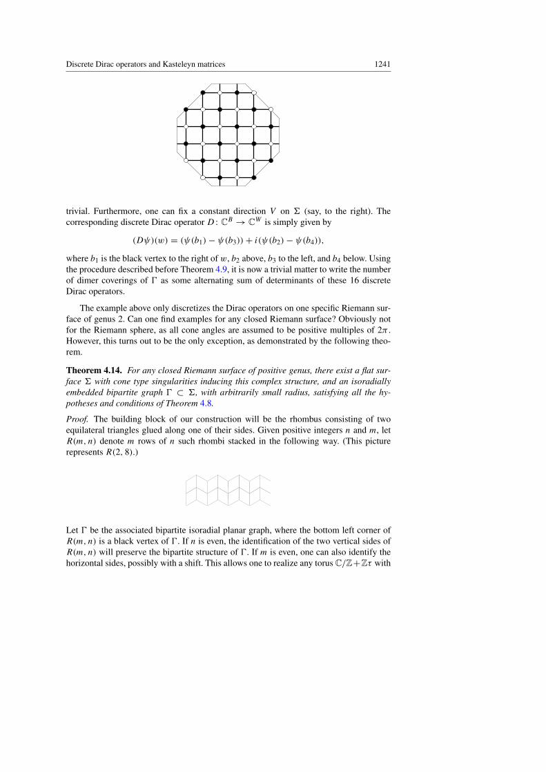
Discrete Dirac operators and Kasteleyn matrices 1241
trivial. Furthermore, one can fix a constant direction V on 6 (say, to the right). Thecorresponding discrete Dirac operator D : CB → CW is simply given by
(Dψ)(w) = (ψ(b1)− ψ(b3))+ i(ψ(b2)− ψ(b4)),
where b1 is the black vertex to the right of w, b2 above, b3 to the left, and b4 below. Usingthe procedure described before Theorem 4.9, it is now a trivial matter to write the numberof dimer coverings of 0 as some alternating sum of determinants of these 16 discreteDirac operators.
The example above only discretizes the Dirac operators on one specific Riemann sur-face of genus 2. Can one find examples for any closed Riemann surface? Obviously notfor the Riemann sphere, as all cone angles are assumed to be positive multiples of 2π .However, this turns out to be the only exception, as demonstrated by the following theo-rem.
Theorem 4.14. For any closed Riemann surface of positive genus, there exist a flat sur-face 6 with cone type singularities inducing this complex structure, and an isoradiallyembedded bipartite graph 0 ⊂ 6, with arbitrarily small radius, satisfying all the hy-potheses and conditions of Theorem 4.8.
Proof. The building block of our construction will be the rhombus consisting of twoequilateral triangles glued along one of their sides. Given positive integers n and m, letR(m, n) denote m rows of n such rhombi stacked in the following way. (This picturerepresents R(2, 8).)
Let 0 be the associated bipartite isoradial planar graph, where the bottom left corner ofR(m, n) is a black vertex of 0. If n is even, the identification of the two vertical sides ofR(m, n) will preserve the bipartite structure of 0. If m is even, one can also identify thehorizontal sides, possibly with a shift. This allows one to realize any torus C/Z+Zτ with

1242 David Cimasoni
τ in some dense subset of H. To obtain all tori, continuously deform one or two rows ofrhombi as illustrated below.
The deformation of two rows changes the imaginary part of τ , while the deforma-tion of a single row changes both the imaginary and the real parts. Therefore, a suitablecombination of these transformations allows one to construct all tori. These examples areflat tori with no singularity, so they trivially satisfy the first condition in Theorem 4.8.Furthermore, one easily checks that condition (ii) is also satisfied, provided n and m aredivisible by 6. (Note that the deformations above do not affect these conditions.)
Let us now consider a fixed positive even integer n. Given three positive integersm1, m2, m3, glue the corresponding rectangles R(m1, n), R(m2, n) and R(m3, n) alongtheir bottom side to an equilateral triangle, itself tiled by rhombi, as illustrated below.
Identifying the opposite remaining sides of each rectangle yields a flat pair of pants witha single singularity of angle 4π . By varying the mj ’s and using the deformation alongtwo rows described above, one can realize any complex structure on the pair of pants.Finally, gluing 2g−2 such pairs of pants along their boundaries (with a possible shift and

Discrete Dirac operators and Kasteleyn matrices 1243
a possible deformation yielding a twist), one can realize any Riemann surface of genusg ≥ 2.
To each rhombus, associate the portion of a bipartite graph 0 given by .
(This is just to avoid cumbersome considerations about gluing bipartite structures.) Thesingularities of angle 4π are located at black vertices of 0, so condition (i) is satisfied.One easily checks that condition (ii) is always satisfied for cycles coming from boundarycomponents of the pairs of pants. Finally, by chosing wisely the parity of the mi’s, onecan ensure that condition (ii) also holds for the cycles passing through several pairs ofpants. ut
Acknowledgments. The author would like to thank Mathieu Baillif, Giovanni Felder and NicolaiReshetikhin for useful discussions.
References
[1] Alvarez-Gaume, L., Moore, G., Vafa, C.: Theta functions, modular invariance, and strings.Comm. Math. Phys. 106, 1–40 (1986) Zbl 0605.58049 MR 0853977
[2] Atiyah, M. F.: Riemann surfaces and spin structures. Ann. Sci. Ecole Norm. Sup. (4) 4, 47–62(1971) Zbl 0212.56402 MR 0286136
[3] Chelkak, D., Smirnov, S.: Discrete complex analysis on isoradial graphs. Adv. Math. 228,1590–1630 (2011) Zbl pre05949114 MR 2824564
[4] Cimasoni, D.: Dimers on graphs in non-orientable surfaces. Lett. Math. Phys. 87, 149–179(2009) Zbl 1167.82006 MR 2480651
[5] Cimasoni, D., Reshetikhin, N.: Dimers on surface graphs and spin structures. I. Comm. Math.Phys. 275, 187–208 (2007) Zbl 1135.82006 MR 2335773
[6] Costa-Santos, R., McCoy, B. M.: Dimers and the critical Ising model on lattices of genus> 1.Nuclear Phys. B 623, 439–473 (2002) Zbl 1097.82518 MR 1883057
[7] Duffin, R. J.: Potential theory on a rhombic lattice. J. Combin. Theory 5, 258–272 (1968)Zbl 0247.31003 MR 0232005
[8] Dynnikov, I. A., Novikov, S. P.: Geometry of the triangle equation on two-manifolds. MoscowMath. J. 3, 419–438, 742 (2003) Zbl 1046.39016 MR 2025267
[9] Ferdinand, A.: Statistical mechanics of dimers on a quadratic lattice. J. Math. Phys. 8, 2332–2339 (1967)
[10] Galluccio, A., Loebl, M.: On the theory of Pfaffian orientations. I. Perfect matchings and per-manents. Electron. J. Combin. 6, res. paper 6, 18 pp. (1999) Zbl 0909.05005 MR 1670286
[11] Johnson, D.: Spin structures and quadratic forms on surfaces. J. London Math. Soc. (2) 22,365–373 (1980) Zbl 0454.57011 MR 0588283
[12] Kasteleyn, P. W.: The statistics of dimers on a lattice. Phys. 27, 1209–1225 (1961)[13] Kasteleyn, P. W.: Dimer statistics and phase transitions. J. Math. Phys. 4, 287–293 (1963)
MR 0153427[14] Kasteleyn, P. W.: Graph theory and crystal physics. In: Graph Theory and Theoretical Physics,
Academic Press, London, 43–110 (1967) Zbl 0205.28402 MR 0253689[15] Kenyon, R.: The Laplacian and Dirac operators on critical planar graphs. Invent. Math. 150,
409–439 (2002) Zbl 1038.58037 MR 1933589[16] Kuperberg, G.: An exploration of the permanent-determinant method. Electron. J. Combin. 5,
res. paper 46, 34 pp. (1998) Zbl 0906.05055 MR 1663576

1244 David Cimasoni
[17] Mercat, C.: Discrete Riemann surfaces and the Ising model. Comm. Math. Phys. 218, 177–216(2001) Zbl 1043.82005 MR 1824204
[18] Tesler, G.: Matchings in graphs on non-orientable surfaces. J. Combin. Theory Ser. B 78,198–231 (2000) Zbl 1025.05052 MR 1750896
[19] Troyanov, M.: Les surfaces euclidiennes a singularites coniques. Enseign. Math. (2) 32, 79–94(1986) Zbl 0611.53035 MR 0850552


![R for MATLAB [AND IGOR] · PDF filehelp(Syntax) help - Command Help: Programming: Operators Matrices, see help for 'MatrixOP' Help on operator syntax Arithmetic operators R/S-Plus](https://img.pdfslide.us/doc/110x75/5a7168307f8b9a9d538cd6a3/r-for-matlab-and-igor-userswwwigorexchangecomfilesmatlab2igorpropdfpdf.jpg)