Embed Size (px)
Citation preview

[Part 4] 1/43
Discrete Choice ModelingBivariate & Multivariate Probit
Discrete Choice Modeling
William Greene
Stern School of Business
New York University
0 Introduction
1 Summary
2 Binary Choice
3 Panel Data
4 Bivariate Probit
5 Ordered Choice
6 Count Data
7 Multinomial Choice
8 Nested Logit
9 Heterogeneity
10 Latent Class
11 Mixed Logit
12 Stated Preference
13 Hybrid Choice

[Part 4] 2/43
Discrete Choice ModelingBivariate & Multivariate Probit
Multivariate Binary Choice Models
Bivariate Probit Models Analysis of bivariate choices
Marginal effects
Prediction
Simultaneous Equations and Recursive Models
A Sample Selection Bivariate Probit Model
The Multivariate Probit Model Specification
Simulation based estimation
Inference
Partial effects and analysis
The ‘panel probit model’

[Part 4] 3/43
Discrete Choice ModelingBivariate & Multivariate Probit
Application: Health Care Usage
German Health Care Usage Data, 7,293 Individuals, Varying Numbers of Periods
Variables in the file are
Data downloaded from Journal of Applied Econometrics Archive. This is an unbalanced panel with 7,293
individuals. They can be used for regression, count models, binary choice, ordered choice, and bivariate binary
choice. This is a large data set. There are altogether 27,326 observations. The number of observations ranges
from 1 to 7. (Frequencies are: 1=1525, 2=1079, 3=825, 4=926, 5=1051, 6=1000, 7=887). Note, the variable
NUMOBS below tells how many observations there are for each person. This variable is repeated in each row of
the data for the person.
DOCTOR = 1(Number of doctor visits > 0)
HOSPITAL = 1(Number of hospital visits > 0)
HSAT = health satisfaction, coded 0 (low) - 10 (high)
DOCVIS = number of doctor visits in last three months
HOSPVIS = number of hospital visits in last calendar year
PUBLIC = insured in public health insurance = 1; otherwise = 0
ADDON = insured by add-on insurance = 1; otherswise = 0
HHNINC = household nominal monthly net income in German marks / 10000.
(4 observations with income=0 were dropped)
HHKIDS = children under age 16 in the household = 1; otherwise = 0
EDUC = years of schooling
AGE = age in years
MARRIED = marital status
EDUC = years of education
[Part 4] 4/43
Discrete Choice ModelingBivariate & Multivariate Probit
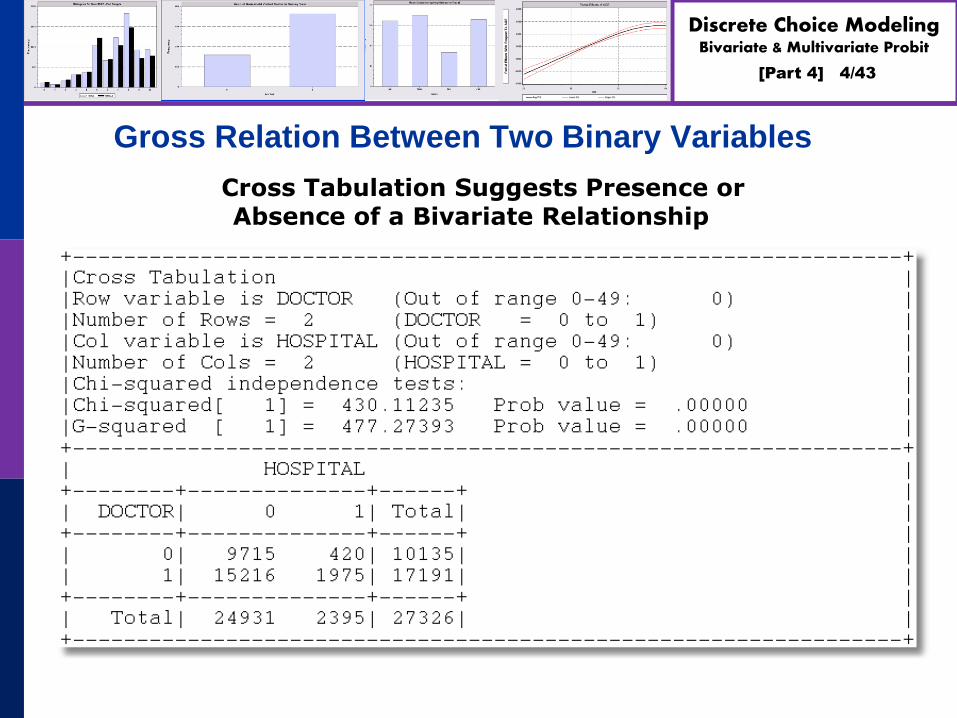
Gross Relation Between Two Binary Variables
Cross Tabulation Suggests Presence or Absence of a Bivariate Relationship

[Part 4] 5/43
Discrete Choice ModelingBivariate & Multivariate Probit
Tetrachoric Correlation
1 1 1 1 1
2 2 2 2 2
1
2
1
A correlation measure for two binary variables
Can be defined implicitly
y * =μ +ε , y =1(y * > 0)
y * =μ +ε ,y =1(y * > 0)
ε 0 1 ρ~ N ,
ε 0 ρ 1
ρ is the between y andtetrachoric correlation 2 y

[Part 4] 6/43
Discrete Choice ModelingBivariate & Multivariate Probit
Log Likelihood Function
n
2 i1 1 i2 2 i1 i2i=1
n
2 i1 1 i2 2 i1 i2i=1
i1 i1 i1 i1
2
logL = logΦ (2y -1)μ ,(2y -1)μ ,(2y -1)(2y -1)ρ
= logΦ q μ ,q μ ,q q ρ
Note : q = (2y -1) = -1 if y = 0 and +1 if y = 1.
Φ =Bivariate normal CDF - must be computed
using qu
1 2
adrature
Maximized with respect to μ ,μ and ρ.

[Part 4] 7/43
Discrete Choice ModelingBivariate & Multivariate Probit
Estimation+---------------------------------------------+
| FIML Estimates of Bivariate Probit Model |
| Maximum Likelihood Estimates |
| Dependent variable DOCHOS |
| Weighting variable None |
| Number of observations 27326 |
| Log likelihood function -25898.27 |
| Number of parameters 3 |
+---------------------------------------------+
+---------+--------------+----------------+--------+---------+
|Variable | Coefficient | Standard Error |b/St.Er.|P[|Z|>z] |
+---------+--------------+----------------+--------+---------+
Index equation for DOCTOR
Constant .32949128 .00773326 42.607 .0000
Index equation for HOSPITAL
Constant -1.35539755 .01074410 -126.153 .0000
Tetrachoric Correlation between DOCTOR and HOSPITAL
RHO(1,2) .31105965 .01357302 22.918 .0000

[Part 4] 8/43
Discrete Choice ModelingBivariate & Multivariate Probit
A Bivariate Probit Model
Two Equation Probit Model
(More than two equations comes later)
No bivariate logit – there is no
reasonable bivariate counterpart
Why fit the two equation model?
Analogy to SUR model: Efficient
Make tetrachoric correlation conditional on
covariates – i.e., residual correlation

[Part 4] 9/43
Discrete Choice ModelingBivariate & Multivariate Probit
Bivariate Probit Model
1 1 1 1 1 1
2 2 2 2 2 2
1
2
2 2
y * = + ε , y =1(y * > 0)
y * = + ε ,y =1(y * > 0)
ε 0 1 ρ~ N ,
ε 0 ρ 1
The variables in and may be the same or
different. There is no need for each equation to have
its 'own vari
β x
β x
x x
.1 2
able.'
ρ is the conditional tetrachoric correlation between y and y
(The equations can be fit one at a time. Use FIML for
(1) efficiency and (2) to get the estimate of ρ.)

[Part 4] 10/43
Discrete Choice ModelingBivariate & Multivariate Probit
ML Estimation of the
Bivariate Probit Model
i1 1 i1n
2 i2 2 i2i=1
i1 i2
n
2 i1 1 i1 i2 2 i2 i1 i2i=1
i1 i1 i1 i1
2
(2y -1) ,
logL = logΦ (2y -1) ,
(2y -1)(2y -1)ρ
= logΦ q ,q ,q q ρ
Note : q = (2y -1) = -1 if y = 0 and +1 if y = 1.
Φ =Bivariate normal CDF - must b
β x
β x
β x β x
1 2
e computed
using quadrature
Maximized with respect to , and ρ.β β

[Part 4] 11/43
Discrete Choice ModelingBivariate & Multivariate Probit
Application to Health Care Data
x1=one,age,female,educ,married,working
x2=one,age,female,hhninc,hhkids
BivariateProbit ;lhs=doctor,hospital
;rh1=x1
;rh2=x2;marginal effects $
[Part 4] 12/43
Discrete Choice ModelingBivariate & Multivariate Probit
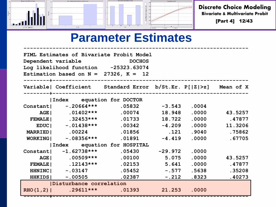
Parameter Estimates----------------------------------------------------------------------
FIML Estimates of Bivariate Probit Model
Dependent variable DOCHOS
Log likelihood function -25323.63074
Estimation based on N = 27326, K = 12
--------+-------------------------------------------------------------
Variable| Coefficient Standard Error b/St.Er. P[|Z|>z] Mean of X
--------+-------------------------------------------------------------
|Index equation for DOCTOR
Constant| -.20664*** .05832 -3.543 .0004
AGE| .01402*** .00074 18.948 .0000 43.5257
FEMALE| .32453*** .01733 18.722 .0000 .47877
EDUC| -.01438*** .00342 -4.209 .0000 11.3206
MARRIED| .00224 .01856 .121 .9040 .75862
WORKING| -.08356*** .01891 -4.419 .0000 .67705
|Index equation for HOSPITAL
Constant| -1.62738*** .05430 -29.972 .0000
AGE| .00509*** .00100 5.075 .0000 43.5257
FEMALE| .12143*** .02153 5.641 .0000 .47877
HHNINC| -.03147 .05452 -.577 .5638 .35208
HHKIDS| -.00505 .02387 -.212 .8323 .40273
|Disturbance correlation
RHO(1,2)| .29611*** .01393 21.253 .0000
--------+-------------------------------------------------------------

[Part 4] 13/43
Discrete Choice ModelingBivariate & Multivariate Probit
Marginal Effects
What are the marginal effects Effect of what on what?
Two equation model, what is the conditional mean?
Possible margins? Derivatives of joint probability = Φ2(β1’xi1, β2’xi2,ρ)
Partials of E[yij|xij] =Φ(βj’xij) (Univariate probability)
Partials of E[yi1|xi1,xi2,yi2=1] = P(yi1,yi2=1)/Prob[yi2=1]
Note marginal effects involve both sets of regressors. If there are common variables, there are two effects in the derivative that are added.
[Part 4] 14/43
Discrete Choice ModelingBivariate & Multivariate Probit
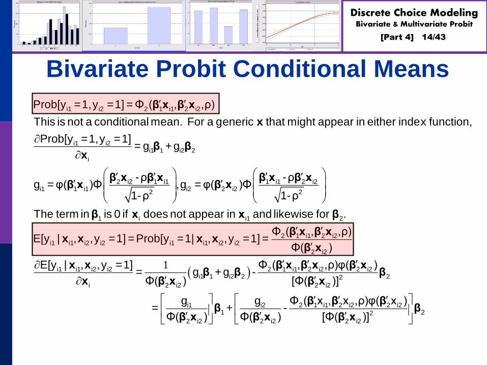
Bivariate Probit Conditional Means
i1 i2 2 1 i1 2 i2
i1 i2i1 1 i2 2
i
2 i2 1 i1i1 1 i1
2
Prob[y =1,y =1] = Φ ( , ,ρ)
This is not a conditional mean. For a generic that might appear in either index function,
Prob[y =1,y =1]= g +g
-ρg = φ( )Φ
1-ρ
β x β x
x
β βx
β x β xβ x
1 i1 2 i2i2 2 i2
2
1 i i1 2
2 1 i1 2 i2i1 i1 i2 i2 i1 i1 i2 i2
2 i2
i1 i1 i
-ρ,g = φ( )Φ
1-ρ
The term in is 0 if does not appear in and likewise for .
Φ ( , ,ρ)E[y | , ,y =1] =Prob[y =1| , ,y =1] =
Φ( )
E[y | ,
β x β xβ x
β x x β
β x β xx x x x
β x
x x
1
2 i2 2 1 i1 2 i2 2 i2i1 1 i2 2 22
i 2 i2 2 i2
i1 i2 2 1 i1 2 i2 2 i21 22
2 i2 2 i2 2 i2
,y =1] Φ ( , ,ρ)φ( )= g +g -
Φ( ) [Φ( )]
g g Φ ( x , x ,ρ)φ( x ) = + -
Φ( ) Φ( ) [Φ( )]
β x β x β xβ β β
x β x β x
β β ββ β
β x β x β x

[Part 4] 15/43
Discrete Choice ModelingBivariate & Multivariate Probit
Marginal Effects: Decomposition
+------------------------------------------------------+
| Marginal Effects for Ey1|y2=1 |
+----------+----------+----------+----------+----------+
| Variable | Efct x1 | Efct x2 | Efct z1 | Efct z2 |
+----------+----------+----------+----------+----------+
| AGE | .00383 | -.00035 | .00000 | .00000 |
| FEMALE | .08857 | -.00835 | .00000 | .00000 |
| EDUC | -.00392 | .00000 | .00000 | .00000 |
| MARRIED | .00061 | .00000 | .00000 | .00000 |
| WORKING | -.02281 | .00000 | .00000 | .00000 |
| HHNINC | .00000 | .00217 | .00000 | .00000 |
| HHKIDS | .00000 | .00035 | .00000 | .00000 |
+----------+----------+----------+----------+----------+
[Part 4] 16/43
Discrete Choice ModelingBivariate & Multivariate Probit
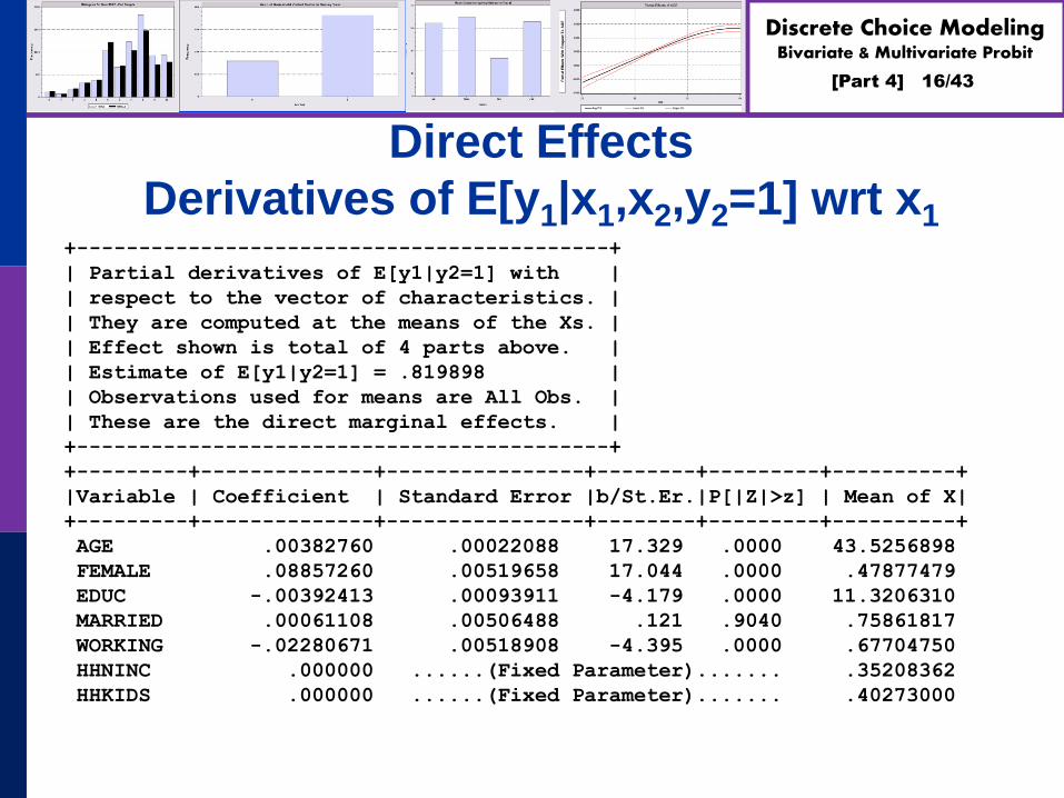
Direct Effects
Derivatives of E[y1|x1,x2,y2=1] wrt x1+-------------------------------------------+
| Partial derivatives of E[y1|y2=1] with |
| respect to the vector of characteristics. |
| They are computed at the means of the Xs. |
| Effect shown is total of 4 parts above. |
| Estimate of E[y1|y2=1] = .819898 |
| Observations used for means are All Obs. |
| These are the direct marginal effects. |
+-------------------------------------------+
+---------+--------------+----------------+--------+---------+----------+
|Variable | Coefficient | Standard Error |b/St.Er.|P[|Z|>z] | Mean of X|
+---------+--------------+----------------+--------+---------+----------+
AGE .00382760 .00022088 17.329 .0000 43.5256898
FEMALE .08857260 .00519658 17.044 .0000 .47877479
EDUC -.00392413 .00093911 -4.179 .0000 11.3206310
MARRIED .00061108 .00506488 .121 .9040 .75861817
WORKING -.02280671 .00518908 -4.395 .0000 .67704750
HHNINC .000000 ......(Fixed Parameter)....... .35208362
HHKIDS .000000 ......(Fixed Parameter)....... .40273000
[Part 4] 17/43
Discrete Choice ModelingBivariate & Multivariate Probit
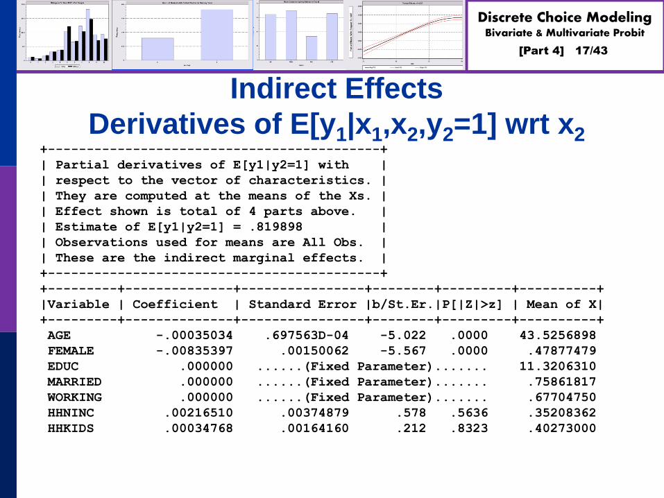
Indirect Effects
Derivatives of E[y1|x1,x2,y2=1] wrt x2+-------------------------------------------+
| Partial derivatives of E[y1|y2=1] with |
| respect to the vector of characteristics. |
| They are computed at the means of the Xs. |
| Effect shown is total of 4 parts above. |
| Estimate of E[y1|y2=1] = .819898 |
| Observations used for means are All Obs. |
| These are the indirect marginal effects. |
+-------------------------------------------+
+---------+--------------+----------------+--------+---------+----------+
|Variable | Coefficient | Standard Error |b/St.Er.|P[|Z|>z] | Mean of X|
+---------+--------------+----------------+--------+---------+----------+
AGE -.00035034 .697563D-04 -5.022 .0000 43.5256898
FEMALE -.00835397 .00150062 -5.567 .0000 .47877479
EDUC .000000 ......(Fixed Parameter)....... 11.3206310
MARRIED .000000 ......(Fixed Parameter)....... .75861817
WORKING .000000 ......(Fixed Parameter)....... .67704750
HHNINC .00216510 .00374879 .578 .5636 .35208362
HHKIDS .00034768 .00164160 .212 .8323 .40273000

[Part 4] 18/43
Discrete Choice ModelingBivariate & Multivariate Probit
Marginal Effects: Total Effects
Sum of Two Derivative Vectors+-------------------------------------------+
| Partial derivatives of E[y1|y2=1] with |
| respect to the vector of characteristics. |
| They are computed at the means of the Xs. |
| Effect shown is total of 4 parts above. |
| Estimate of E[y1|y2=1] = .819898 |
| Observations used for means are All Obs. |
| Total effects reported = direct+indirect. |
+-------------------------------------------+
+---------+--------------+----------------+--------+---------+----------+
|Variable | Coefficient | Standard Error |b/St.Er.|P[|Z|>z] | Mean of X|
+---------+--------------+----------------+--------+---------+----------+
AGE .00347726 .00022941 15.157 .0000 43.5256898
FEMALE .08021863 .00535648 14.976 .0000 .47877479
EDUC -.00392413 .00093911 -4.179 .0000 11.3206310
MARRIED .00061108 .00506488 .121 .9040 .75861817
WORKING -.02280671 .00518908 -4.395 .0000 .67704750
HHNINC .00216510 .00374879 .578 .5636 .35208362
HHKIDS .00034768 .00164160 .212 .8323 .40273000
[Part 4] 19/43
Discrete Choice ModelingBivariate & Multivariate Probit
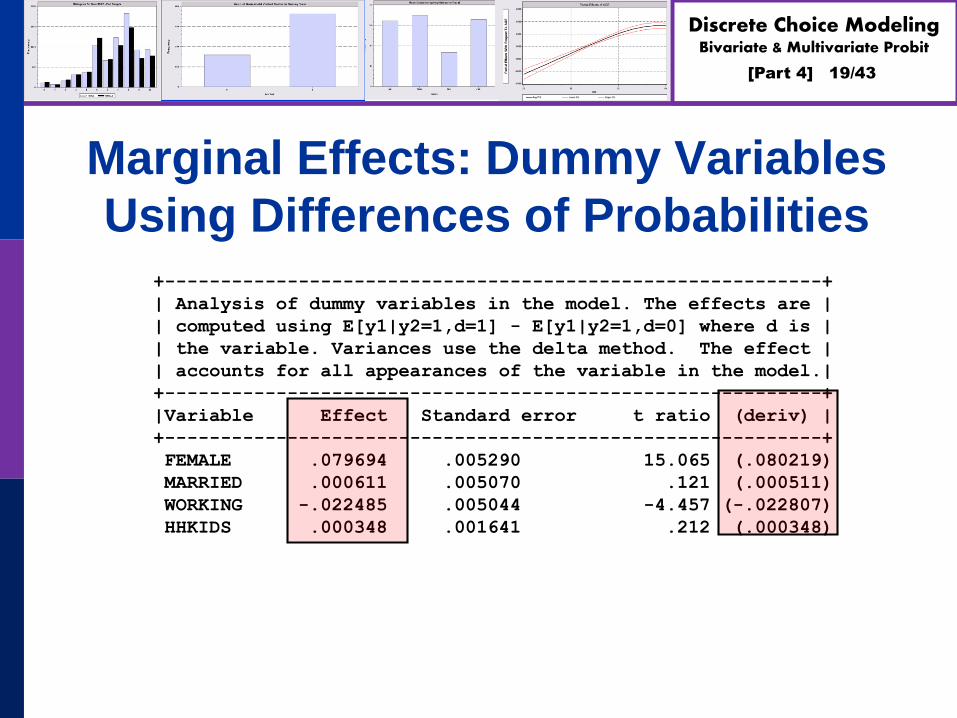
Marginal Effects: Dummy Variables
Using Differences of Probabilities+-----------------------------------------------------------+
| Analysis of dummy variables in the model. The effects are |
| computed using E[y1|y2=1,d=1] - E[y1|y2=1,d=0] where d is |
| the variable. Variances use the delta method. The effect |
| accounts for all appearances of the variable in the model.|
+-----------------------------------------------------------+
|Variable Effect Standard error t ratio (deriv) |
+-----------------------------------------------------------+
FEMALE .079694 .005290 15.065 (.080219)
MARRIED .000611 .005070 .121 (.000511)
WORKING -.022485 .005044 -4.457 (-.022807)
HHKIDS .000348 .001641 .212 (.000348)

[Part 4] 20/43
Discrete Choice ModelingBivariate & Multivariate Probit
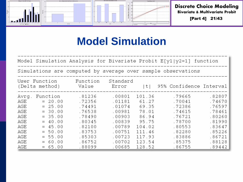
Average Partial Effects
[Part 4] 21/43
Discrete Choice ModelingBivariate & Multivariate Probit
Model Simulation

[Part 4] 22/43
Discrete Choice ModelingBivariate & Multivariate Probit
Model Simulation

[Part 4] 23/43
Discrete Choice ModelingBivariate & Multivariate Probit
A Simultaneous Equations Model
1
1 1 1 2 1 1 1
2 2 2 2 1 2 2 2
1
2
Simultaneous Equations Model
y * = + θ y + ε , y = 1(y * > 0)
y * = + θ y + ε ,y = 1(y * > 0)
ε 0 1 ρ~ N
Incoh
,ε 0
e
ρ 1
T renhis model is not identified.
(Not estimable. The compu
t
an
.
ter c
β x
β x
compute 'estimates' but they have no meaning.)
[Part 4] 24/43
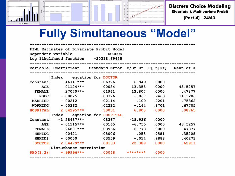
Discrete Choice ModelingBivariate & Multivariate Probit
Fully Simultaneous “Model”----------------------------------------------------------------------
FIML Estimates of Bivariate Probit Model
Dependent variable DOCHOS
Log likelihood function -20318.69455
--------+-------------------------------------------------------------
Variable| Coefficient Standard Error b/St.Er. P[|Z|>z] Mean of X
--------+-------------------------------------------------------------
|Index equation for DOCTOR
Constant| -.46741*** .06726 -6.949 .0000
AGE| .01124*** .00084 13.353 .0000 43.5257
FEMALE| .27070*** .01961 13.807 .0000 .47877
EDUC| -.00025 .00376 -.067 .9463 11.3206
MARRIED| -.00212 .02114 -.100 .9201 .75862
WORKING| -.00362 .02212 -.164 .8701 .67705
HOSPITAL| 2.04295*** .30031 6.803 .0000 .08765
|Index equation for HOSPITAL
Constant| -1.58437*** .08367 -18.936 .0000
AGE| -.01115*** .00165 -6.755 .0000 43.5257
FEMALE| -.26881*** .03966 -6.778 .0000 .47877
HHNINC| .00421 .08006 .053 .9581 .35208
HHKIDS| -.00050 .03559 -.014 .9888 .40273
DOCTOR| 2.04479*** .09133 22.389 .0000 .62911
|Disturbance correlation
RHO(1,2)| -.99996*** .00048 ******** .0000
--------+-------------------------------------------------------------

[Part 4] 25/43
Discrete Choice ModelingBivariate & Multivariate Probit
A Recursive Simultaneous
Equations Model
1 1 1 1 1 1
2 2 2 2 1 2 2 2
1
2
Recursive Simultaneous Equations Model
y * = + ε , y = 1(y * > 0)
y * = + θ y + ε ,y = 1(y * > 0)
ε 0 1 ρ~ N ,
ε 0 ρ 1
This model is identified. It can be consiste
β x
β x
ntly and efficiently
estimated by full information maximum likelihood. Treated as
a bivariate probit model, ignoring the simultaneity.
Bivariate ; Lhs = y1,y2 ; Rh1=…,y2 ; Rh2 = … $

[Part 4] 26/43
Discrete Choice ModelingBivariate & Multivariate Probit
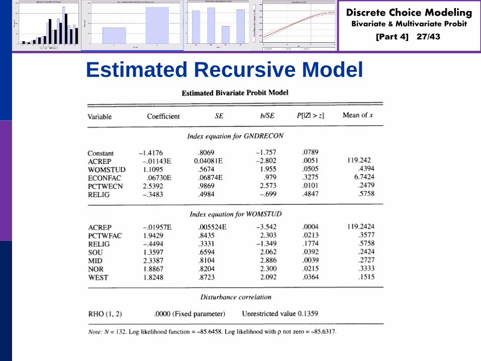
Application: Gender Economics at
Liberal Arts Colleges
Journal of Economic Education, fall, 1998.
[Part 4] 27/43
Discrete Choice ModelingBivariate & Multivariate Probit
Estimated Recursive Model
[Part 4] 28/43
Discrete Choice ModelingBivariate & Multivariate Probit
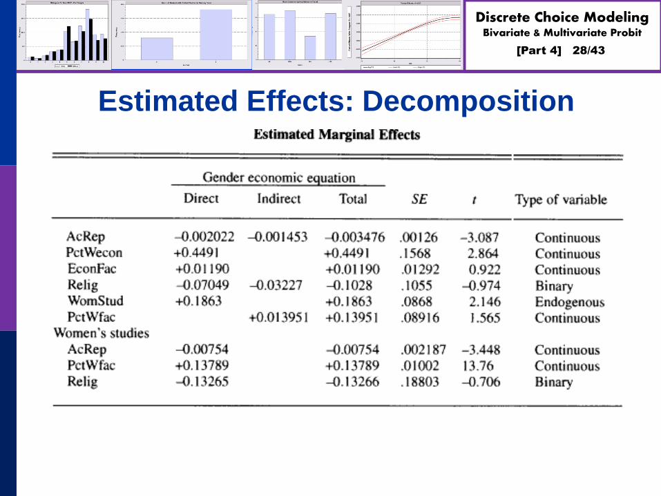
Estimated Effects: Decomposition

[Part 4] 29/43
Discrete Choice ModelingBivariate & Multivariate Probit

[Part 4] 30/43
Discrete Choice ModelingBivariate & Multivariate Probit

[Part 4] 31/43
Discrete Choice ModelingBivariate & Multivariate Probit
Causal Inference?
There is no partial (marginal) effect for PIP.
PIP cannot change partially (marginally). It changes because something
else changes. (X or I or u2.)
The calculation of MEPIP does not make sense.
Causal Inference?
[Part 4] 32/43
Discrete Choice ModelingBivariate & Multivariate Probit

[Part 4] 33/43
Discrete Choice ModelingBivariate & Multivariate Probit

[Part 4] 34/43
Discrete Choice ModelingBivariate & Multivariate Probit

[Part 4] 35/43
Discrete Choice ModelingBivariate & Multivariate Probit

[Part 4] 36/43
Discrete Choice ModelingBivariate & Multivariate Probit

[Part 4] 37/43
Discrete Choice ModelingBivariate & Multivariate Probit
A Sample Selection Model
1 1 1 1 1 1
2 2 2 2 2 2
1
2
1 2
1 2 1 2 2 1 2
Sample Selection Model
y * = + ε , y =1(y * > 0)
y * = + ε ,y =1(y * > 0)
ε 0 1 ρ~ N ,
ε 0 ρ 1
y is only observed when y = 1.
f(y ,y ) = Prob[y =1| y =1] *Prob[y =1] (y =1,y =1)
β x
β x
1 2 2 1 2
2 2
= Prob[y = 0 | y =1] *Prob[y =1] (y = 0,y =1)
= Prob[y = 0] (y = 0)
[Part 4] 38/43
Discrete Choice ModelingBivariate & Multivariate Probit
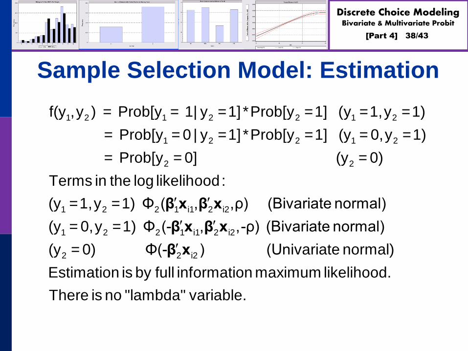
Sample Selection Model: Estimation
1 2 1 2 2 1 2
1 2 2 1 2
2 2
f(y ,y ) = Prob[y = 1| y =1] *Prob[y =1] (y =1,y =1)
= Prob[y = 0 | y =1] *Prob[y =1] (y = 0,y =1)
= Prob[y = 0] (y = 0)
Terms in the log likelih
1 2 2 1 i1 2 i2
1 2 2 1 i1 2 i2
2 2 i2
ood:
(y =1,y =1) Φ ( , ,ρ) (Bivariate normal)
(y = 0,y =1) Φ (- , ,-ρ) (Bivariate normal)
(y = 0) Φ(- ) (Univariate normal)
Estimation is by full inf
β x β x
β x β x
β x
ormation maximum likelihood.
There is no "lambda" variable.

[Part 4] 39/43
Discrete Choice ModelingBivariate & Multivariate Probit
Application: Credit Scoring
American Express: 1992
N = 13,444 Applications
Observed application data
Observed acceptance/rejection of application
N1 = 10,499 Cardholders
Observed demographics and economic data
Observed default or not in first 12 months
Full Sample is in AmEx.lpj; description shows when imported.

[Part 4] 40/43
Discrete Choice ModelingBivariate & Multivariate Probit
The Multivariate Probit Model
1 1 1 1 1 1
2 2 2 2 2 2
M M M M M M
1 12 1M
2 1
M
M
Multiple Equations Analog to SUR Model for M Binary Variables
y * = + ε , y =1(y * > 0)
y * = + ε , y =1(y * > 0)
...
y * = + ε , y =1(y * > 0)
ε 1 ρ ... ρ0
ε ρ0~ N ,
... ...
ε 0
β x
β x
β x
mnΣ *
2 2M
1M 2M
N
M i1 1 i1 i2 2 i2 iM M iMi=1
im in mn
1 ... ρ
... ... ... ...
ρ ρ ... 1
logL = logΦ [q ,q ,...,q | *]
1 if m = n or q q ρ if not.
β x β x β x Σ

[Part 4] 41/43
Discrete Choice ModelingBivariate & Multivariate Probit
MLE: Simulation
Estimation of the multivariate probit model requires evaluation of M-order Integrals
The general case is usually handled with the GHK simulator. Much current research focuses on efficiency (speed) gains in this computation.
The “Panel Probit Model” is a special case. (Bertschek-Lechner, JE, 1999) – Construct a GMM
estimator using only first order integrals of the univariate normal CDF
(Greene, Emp.Econ, 2003) – Estimate the integrals with simulation (GHK) anyway.
[Part 4] 42/43
Discrete Choice ModelingBivariate & Multivariate Probit
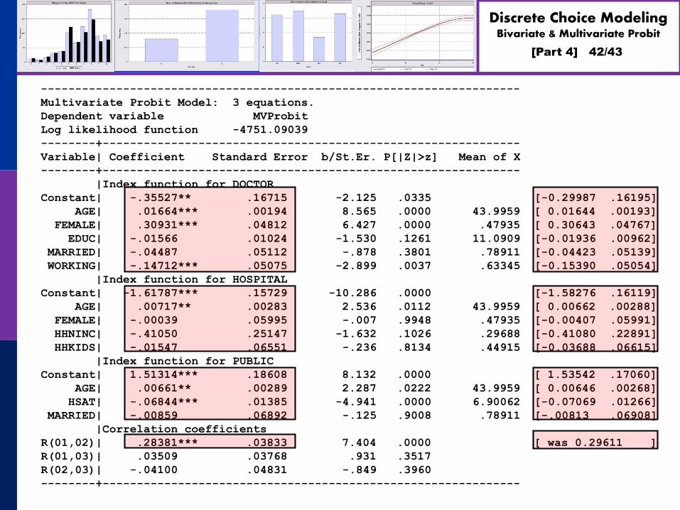
----------------------------------------------------------------------
Multivariate Probit Model: 3 equations.
Dependent variable MVProbit
Log likelihood function -4751.09039
--------+-------------------------------------------------------------
Variable| Coefficient Standard Error b/St.Er. P[|Z|>z] Mean of X
--------+-------------------------------------------------------------
|Index function for DOCTOR
Constant| -.35527** .16715 -2.125 .0335 [-0.29987 .16195]
AGE| .01664*** .00194 8.565 .0000 43.9959 [ 0.01644 .00193]
FEMALE| .30931*** .04812 6.427 .0000 .47935 [ 0.30643 .04767]
EDUC| -.01566 .01024 -1.530 .1261 11.0909 [-0.01936 .00962]
MARRIED| -.04487 .05112 -.878 .3801 .78911 [-0.04423 .05139]
WORKING| -.14712*** .05075 -2.899 .0037 .63345 [-0.15390 .05054]
|Index function for HOSPITAL
Constant| -1.61787*** .15729 -10.286 .0000 [-1.58276 .16119]
AGE| .00717** .00283 2.536 .0112 43.9959 [ 0.00662 .00288]
FEMALE| -.00039 .05995 -.007 .9948 .47935 [-0.00407 .05991]
HHNINC| -.41050 .25147 -1.632 .1026 .29688 [-0.41080 .22891]
HHKIDS| -.01547 .06551 -.236 .8134 .44915 [-0.03688 .06615]
|Index function for PUBLIC
Constant| 1.51314*** .18608 8.132 .0000 [ 1.53542 .17060]
AGE| .00661** .00289 2.287 .0222 43.9959 [ 0.00646 .00268]
HSAT| -.06844*** .01385 -4.941 .0000 6.90062 [-0.07069 .01266]
MARRIED| -.00859 .06892 -.125 .9008 .78911 [-.00813 .06908]
|Correlation coefficients
R(01,02)| .28381*** .03833 7.404 .0000 [ was 0.29611 ]
R(01,03)| .03509 .03768 .931 .3517
R(02,03)| -.04100 .04831 -.849 .3960
--------+-------------------------------------------------------------
[Part 4] 43/43
Discrete Choice ModelingBivariate & Multivariate Probit
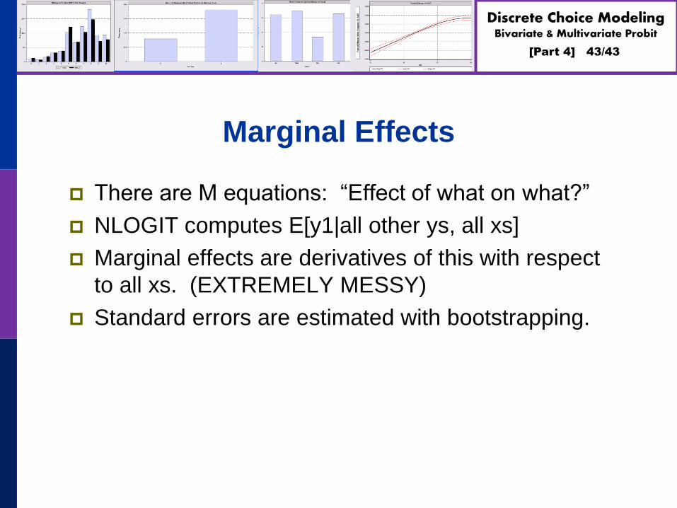
Marginal Effects
There are M equations: “Effect of what on what?”
NLOGIT computes E[y1|all other ys, all xs]
Marginal effects are derivatives of this with respect
to all xs. (EXTREMELY MESSY)
Standard errors are estimated with bootstrapping.


![Part 3: Basic Linear Panel Data Models - New York …people.stern.nyu.edu/.../2014/DC2014-3-PanelRegression.pdf · [Topic 3-Panel Data Regression] 12/97 Cornwell and Rupert Data Cornwell](https://img.pdfslide.us/doc/110x75/5b85f9957f8b9ad1318beaa5/part-3-basic-linear-panel-data-models-new-york-topic-3-panel-data-regression.jpg)


![[Introduction] - WordPress.com · · 2012-06-25Chapter - Introduction Discrete Structures Samujjwal Bhandari 2 Introduction Discrete Mathematics deals with discrete objects. Discrete](https://img.pdfslide.us/doc/110x75/5b18f6f47f8b9a32258c36c3/introduction-2012-06-25chapter-introduction-discrete-structures-samujjwal.jpg)