Embed Size (px)
Citation preview
Discrete and Continuous Dynamical Systems:Applications and Examples
Yonah Borns-Weil and Junho WonMentored by Dr. Aaron Welters
Fourth Annual PRIMES Conference
May 18, 2014
J. Won, Y. Borns-Weil (MIT) Discrete and Continuous Dynamical Systems May 18, 2014 1 / 32
Overview of dynamical systems
What is a dynamical system?
Two flavors:
Discrete (Iterative Maps)
Continuous (Differential Equations)
J. Won, Y. Borns-Weil (MIT) Discrete and Continuous Dynamical Systems May 18, 2014 2 / 32
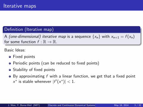
Iterative maps
Definition (Iterative map)
A (one-dimensional) iterative map is a sequence {xn} with xn+1 = f (xn)for some function f : R→ R.
Basic Ideas:
Fixed points
Periodic points (can be reduced to fixed points)
Stability of fixed points
By approximating f with a linear function, we get that a fixed pointx∗ is stable whenever |f ′(x∗)| < 1.
J. Won, Y. Borns-Weil (MIT) Discrete and Continuous Dynamical Systems May 18, 2014 3 / 32
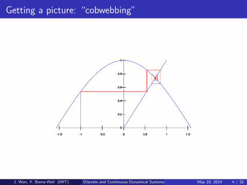
Getting a picture: “cobwebbing”
J. Won, Y. Borns-Weil (MIT) Discrete and Continuous Dynamical Systems May 18, 2014 4 / 32
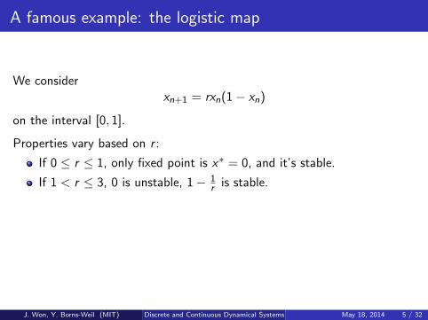
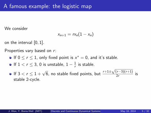
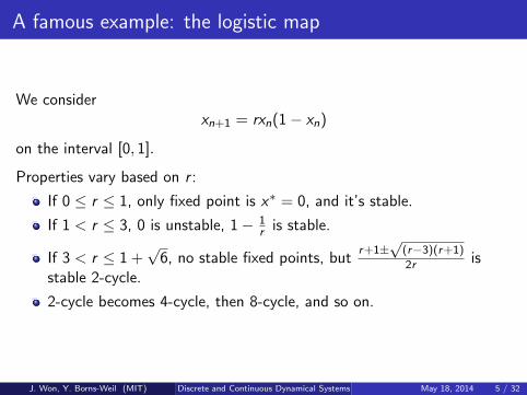
A famous example: the logistic map
We considerxn+1 = rxn(1− xn)
on the interval [0, 1].
Properties vary based on r :
If 0 ≤ r ≤ 1, only fixed point is x∗ = 0, and it’s stable.
If 1 < r ≤ 3, 0 is unstable, 1− 1r is stable.
If 3 < r ≤ 1 +√
6, no stable fixed points, butr+1±√
(r−3)(r+1)
2r isstable 2-cycle.
2-cycle becomes 4-cycle, then 8-cycle, and so on.
J. Won, Y. Borns-Weil (MIT) Discrete and Continuous Dynamical Systems May 18, 2014 5 / 32
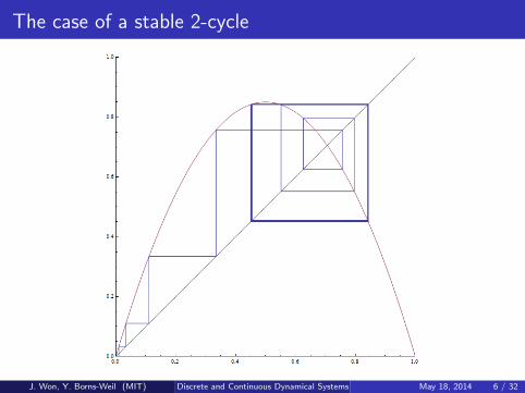
The case of a stable 2-cycle
J. Won, Y. Borns-Weil (MIT) Discrete and Continuous Dynamical Systems May 18, 2014 6 / 32
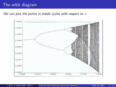
The orbit diagram
We can plot the points in stable cycles with respect to r :
J. Won, Y. Borns-Weil (MIT) Discrete and Continuous Dynamical Systems May 18, 2014 7 / 32
The first Feigenbaum constant
Let rn be where stable 2n cycle begins.The distance between rn’s converges roughly geometrically, up to r∞.
Definition (δ)
The first Feigenbaum constant is defined as
δ = limn→∞
rn − rn−1rn+1 − rn
≈ 4.669 . . .
J. Won, Y. Borns-Weil (MIT) Discrete and Continuous Dynamical Systems May 18, 2014 8 / 32
The first Feigenbaum constant: not just for one map?
Yeah, but why do we care about δ?
Consider the sine mapxn+1 = r sinπxn.
Guess what its orbit diagram looks like?
J. Won, Y. Borns-Weil (MIT) Discrete and Continuous Dynamical Systems May 18, 2014 9 / 32
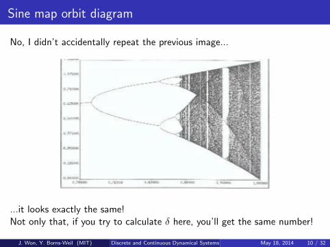
Sine map orbit diagram
No, I didn’t accidentally repeat the previous image...
...it looks exactly the same!Not only that, if you try to calculate δ here, you’ll get the same number!
J. Won, Y. Borns-Weil (MIT) Discrete and Continuous Dynamical Systems May 18, 2014 10 / 32

Univerality of δ
Theorem 1 (Universality of δ)
If
Dschf (x) =
(f ′′
f ′
)′(x)− 1
2
(f ′′(x)
f ′(x)
)2
< 0
in the bounded interval and f experiences period-doubling, then letting{rn} be defined for this new map,
limn→∞
rn − rn−1rn+1 − rn
= δ.
Essentially, δ is a “universal constant!”
J. Won, Y. Borns-Weil (MIT) Discrete and Continuous Dynamical Systems May 18, 2014 11 / 32
Now, the continuous case ...
Continuous dynamical systems involve analyzing differential equations.
They describe systems that change over time.
J. Won, Y. Borns-Weil (MIT) Discrete and Continuous Dynamical Systems May 18, 2014 12 / 32
Oscillating chemical reactions
Chemical reactions: governed by differential equations involvingconcentrations of the reactants and products.
Multi-step reactions can exhibit complicated dynamical behaviors.
Belousov’s discovery in 1950’s exhibits a periodical behavior.
J. Won, Y. Borns-Weil (MIT) Discrete and Continuous Dynamical Systems May 18, 2014 13 / 32
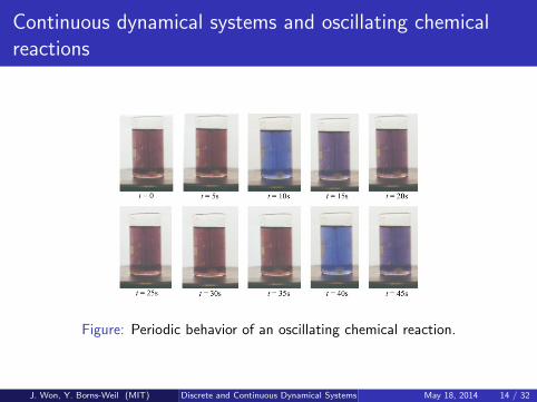
Continuous dynamical systems and oscillating chemicalreactions
Figure: Periodic behavior of an oscillating chemical reaction.
J. Won, Y. Borns-Weil (MIT) Discrete and Continuous Dynamical Systems May 18, 2014 14 / 32
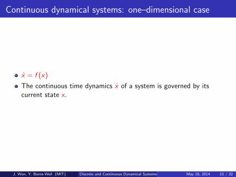
Continuous dynamical systems: one–dimensional case
x = f (x)
The continuous time dynamics x of a system is governed by itscurrent state x.
J. Won, Y. Borns-Weil (MIT) Discrete and Continuous Dynamical Systems May 18, 2014 15 / 32
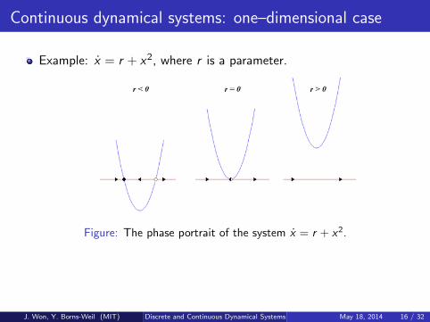
Continuous dynamical systems: one–dimensional case
Example: x = r + x2, where r is a parameter.
Figure: The phase portrait of the system x = r + x2.
Flow and vector fields
Stable and unstable fixed points (x = 0)
J. Won, Y. Borns-Weil (MIT) Discrete and Continuous Dynamical Systems May 18, 2014 16 / 32
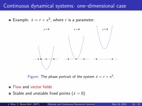
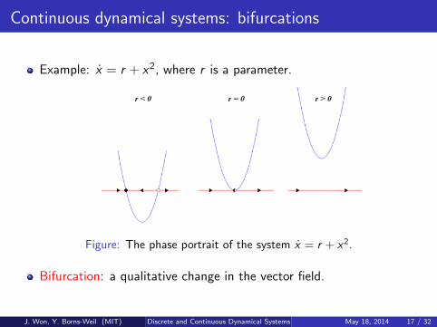
Continuous dynamical systems: bifurcations
Example: x = r + x2, where r is a parameter.
Figure: The phase portrait of the system x = r + x2.
Bifurcation: a qualitative change in the vector field.
J. Won, Y. Borns-Weil (MIT) Discrete and Continuous Dynamical Systems May 18, 2014 17 / 32
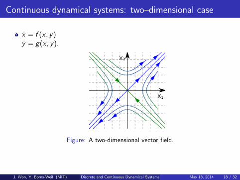
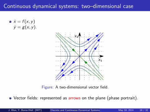
Continuous dynamical systems: two–dimensional case
x = f (x , y)y = g(x , y).
Figure: A two-dimensional vector field.
Vector fields: represented as arrows on the plane (phase portrait).
J. Won, Y. Borns-Weil (MIT) Discrete and Continuous Dynamical Systems May 18, 2014 18 / 32
Continuous dynamical systems: two–dimensional case
x = f (x , y)y = g(x , y).
Figure: A two-dimensional vector field.
Vector fields: represented as arrows on the plane (phase portrait).
J. Won, Y. Borns-Weil (MIT) Discrete and Continuous Dynamical Systems May 18, 2014 18 / 32
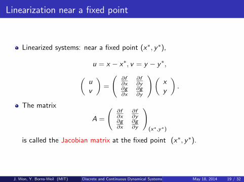
Linearization near a fixed point
Linearized systems: near a fixed point (x∗, y∗),
u = x − x∗, v = y − y∗,(uv
)=
(∂f∂x
∂f∂y
∂g∂x
∂g∂y
)(xy
).
The matrix
A =
(∂f∂x
∂f∂y
∂g∂x
∂g∂y
)(x∗,y∗)
is called the Jacobian matrix at the fixed point (x∗, y∗).
J. Won, Y. Borns-Weil (MIT) Discrete and Continuous Dynamical Systems May 18, 2014 19 / 32
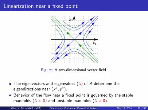
Linearization near a fixed point
Figure: A two-dimensional vector field.
The eigenvectors and eigenvalues (λ) of A determine theeigendirections near (x∗, y∗).
Behavior of the flow near a fixed point is governed by the stablemanifolds (λ < 0) and unstable manifolds (λ > 0).
J. Won, Y. Borns-Weil (MIT) Discrete and Continuous Dynamical Systems May 18, 2014 20 / 32
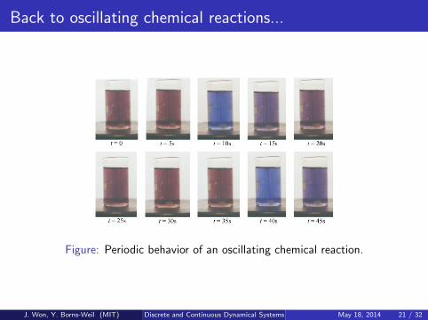
Back to oscillating chemical reactions...
Figure: Periodic behavior of an oscillating chemical reaction.
J. Won, Y. Borns-Weil (MIT) Discrete and Continuous Dynamical Systems May 18, 2014 21 / 32
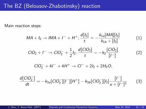
The BZ (Belousov-Zhabotinsky) reaction
Main reaction steps:
MA + I2 → IMA + I− + H+;d [I2]
t= −k1a[MA][I2]
k1b + [I2](1)
ClO2 + I− → ClO−2 +1
2I2;
d [ClO2]
t= −k2
[ClO2]
[I−](2)
ClO−2 + 4I− + 4H+ → Cl− + 2I2 + 2H2O;
d [ClO−2 ]
dt= −k3a[ClO−2 ][I−][H+]− k3b[ClO−2 ][I2]
[I−]
u + [I−]2(3)
J. Won, Y. Borns-Weil (MIT) Discrete and Continuous Dynamical Systems May 18, 2014 22 / 32
The BZ (Belousov-Zhabotinsky) reaction
Main reaction steps:
MA + I2 → IMA + I− + H+;d [I2]
t= −k1a[MA][I2]
k1b + [I2](4)
ClO2 + I− → ClO−2 +1
2I2;
d [ClO2]
t= −k2
[ClO2]
[I−](5)
ClO−2 + 4I− + 4H+ → Cl− + 2I2 + 2H2O;
d [ClO−2 ]
dt= −k3a[ClO−2 ][I−][H+]− k3b[ClO−2 ][I2]
[I−]
u + [I−]2(6)
=⇒Very complicated.
J. Won, Y. Borns-Weil (MIT) Discrete and Continuous Dynamical Systems May 18, 2014 23 / 32
Simplified model of the BZ reaction
x = a− x − 4xy1+x2
,
y = bx(
1− y1+x2
).
Here, x and y are dimensionless concentrations of I− and ClO−2 .
J. Won, Y. Borns-Weil (MIT) Discrete and Continuous Dynamical Systems May 18, 2014 24 / 32
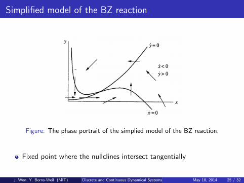
Simplified model of the BZ reaction
Figure: The phase portrait of the simplied model of the BZ reaction.
Fixed point where the nullclines intersect tangentially
J. Won, Y. Borns-Weil (MIT) Discrete and Continuous Dynamical Systems May 18, 2014 25 / 32
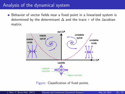
Analysis of the dynamical system
Behavior of vector fields near a fixed point in a linearized system isdetermined by the determinant ∆ and the trace τ of the Jacobianmatrix.
Figure: Classification of fixed points.
J. Won, Y. Borns-Weil (MIT) Discrete and Continuous Dynamical Systems May 18, 2014 26 / 32
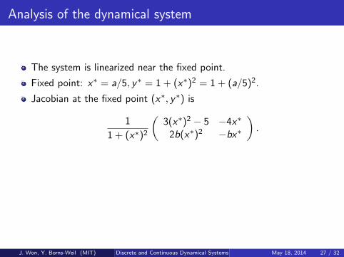
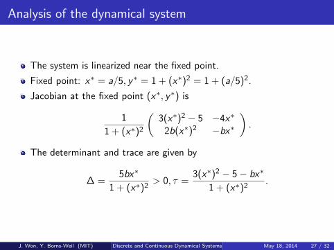
Analysis of the dynamical system
The system is linearized near the fixed point.
Fixed point: x∗ = a/5, y∗ = 1 + (x∗)2 = 1 + (a/5)2.
Jacobian at the fixed point (x∗, y∗) is
1
1 + (x∗)2
(3(x∗)2 − 5 −4x∗
2b(x∗)2 −bx∗).
The determinant and trace are given by
∆ =5bx∗
1 + (x∗)2> 0, τ =
3(x∗)2 − 5− bx∗
1 + (x∗)2.
J. Won, Y. Borns-Weil (MIT) Discrete and Continuous Dynamical Systems May 18, 2014 27 / 32
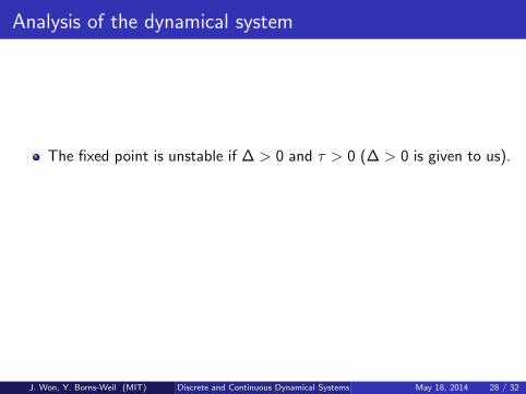
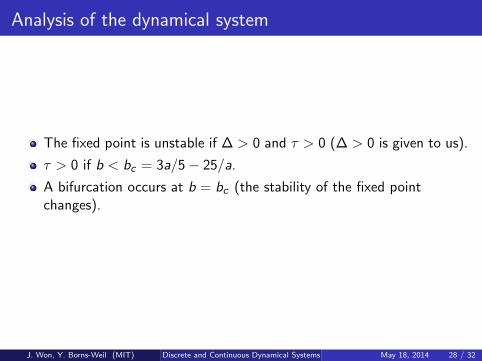
Analysis of the dynamical system
The fixed point is unstable if ∆ > 0 and τ > 0 (∆ > 0 is given to us).
τ > 0 if b < bc = 3a/5− 25/a.
A bifurcation occurs at b = bc (the stability of the fixed pointchanges).
J. Won, Y. Borns-Weil (MIT) Discrete and Continuous Dynamical Systems May 18, 2014 28 / 32
Analysis of the dynamical system
The fixed point is unstable if ∆ > 0 and τ > 0 (∆ > 0 is given to us).
τ > 0 if b < bc = 3a/5− 25/a.
A bifurcation occurs at b = bc (the stability of the fixed pointchanges).
J. Won, Y. Borns-Weil (MIT) Discrete and Continuous Dynamical Systems May 18, 2014 28 / 32
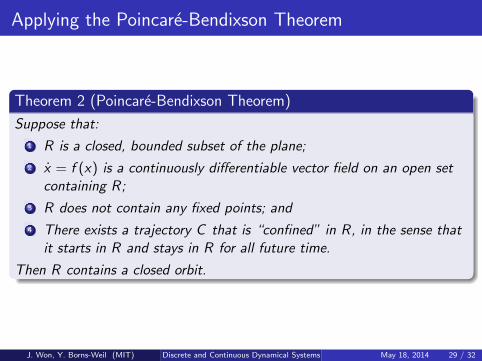
Applying the Poincare-Bendixson Theorem
Theorem 2 (Poincare-Bendixson Theorem)
Suppose that:
1 R is a closed, bounded subset of the plane;
2 x = f (x) is a continuously differentiable vector field on an open setcontaining R;
3 R does not contain any fixed points; and
4 There exists a trajectory C that is “confined” in R, in the sense thatit starts in R and stays in R for all future time.
Then R contains a closed orbit.
J. Won, Y. Borns-Weil (MIT) Discrete and Continuous Dynamical Systems May 18, 2014 29 / 32
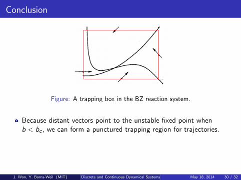
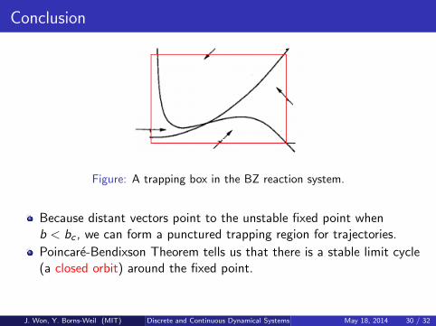
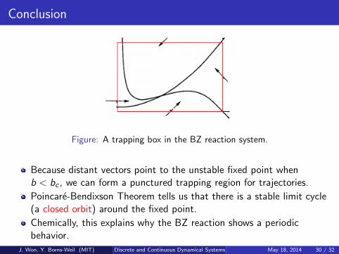
Conclusion
Figure: A trapping box in the BZ reaction system.
Because distant vectors point to the unstable fixed point whenb < bc , we can form a punctured trapping region for trajectories.
Poincare-Bendixson Theorem tells us that there is a stable limit cycle(a closed orbit) around the fixed point.
Chemically, this explains why the BZ reaction shows a periodicbehavior.
J. Won, Y. Borns-Weil (MIT) Discrete and Continuous Dynamical Systems May 18, 2014 30 / 32
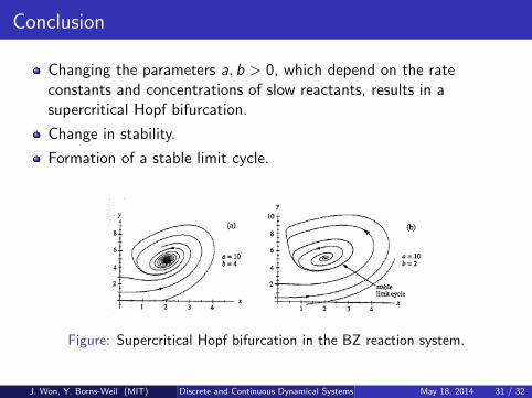
Conclusion
Changing the parameters a, b > 0, which depend on the rateconstants and concentrations of slow reactants, results in asupercritical Hopf bifurcation.
Change in stability.
Formation of a stable limit cycle.
Figure: Supercritical Hopf bifurcation in the BZ reaction system.
J. Won, Y. Borns-Weil (MIT) Discrete and Continuous Dynamical Systems May 18, 2014 31 / 32

Bibliography
S. H. Strogatz,Nonlinear Dynamics and Chaos,Perseus Books Publishing, Cambridge, 1994.
J. Won, Y. Borns-Weil (MIT) Discrete and Continuous Dynamical Systems May 18, 2014 31 / 32

Acknowledgements
We thank our mentor Dr. Aaron Welters for mentoring us with studyingnonlinear dynamical systems, as well as providing many useful advice ingeneral. Also, our head mentor Dr. Tanya Khovanova and others havehelped us with improving our presentation, and MIT—PRIMES providedus with this enjoyable opportunity to study mathematics. Finally, we wishto thank our parents for their continued support with our studies.
J. Won, Y. Borns-Weil (MIT) Discrete and Continuous Dynamical Systems May 18, 2014 32 / 32