Embed Size (px)
Citation preview
C. Phillips, Centre de C. Phillips, Centre de RecherchesRecherches du Cyclotron, ULg, Belgiumdu Cyclotron, ULg, Belgium
Multiple comparison problemMultiple Multiple comparisoncomparison problemproblem
DISCOS SPM course, CRC, Liège, 2009DISCOS SPM course, CRC, LiDISCOS SPM course, CRC, Lièège, 2009ge, 2009
Based on slides from: T. Nichols
ContentsContentsContents
• Recap & Introduction
• Inference & multiple comparison
• « Take home » message
•• RecapRecap & Introduction & Introduction
•• InferenceInference & multiple & multiple comparisoncomparison
•• «« TakeTake homehome »» messagemessage
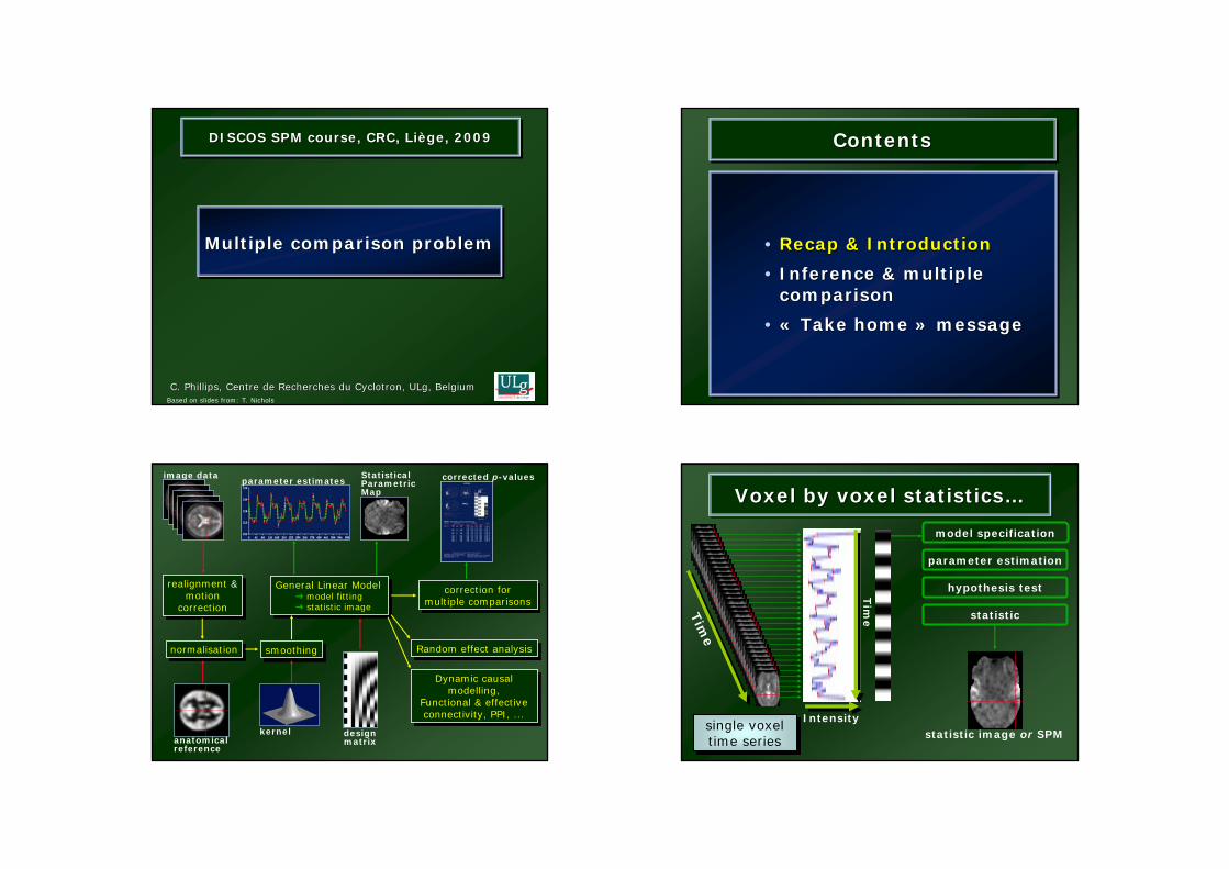
realignment &motion
correction
realignment &motion
correction
smoothingsmoothingnormalisationnormalisation
General Linear Modelmodel fittingstatistic image
General Linear Modelmodel fittingstatistic image
corrected p-valuesparameter estimates
anatomical reference
kernel
image data
designmatrix
StatisticalParametric Map
correction for multiple comparisons
correction for multiple comparisons
Random effect analysisRandom effect analysis
Dynamic causal modelling,
Functional & effective connectivity, PPI, ...
Dynamic causal modelling,
Functional & effective connectivity, PPI, ...
Voxel by voxel statistics…Voxel by voxel statisticsVoxel by voxel statistics……
parameter estimation
hypothesis test
statistic image or SPM
statisticTim
e
Intensity
Tim
e
single voxeltime series
single voxeltime series
model specification
General Linear Model (in SPM)General Linear Model General Linear Model (in SPM)(in SPM)
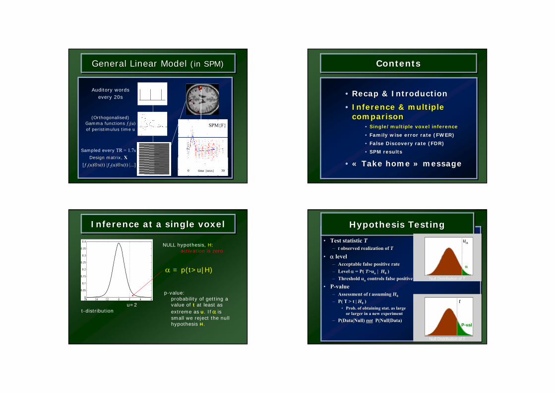
Auditory words every 20s
SPMFSPMF
0 time 0 time secssecs 30 30
Sampled every TR = 1.7sDesign matrix,Design matrix, XX
[[ƒƒ11(u)(u)⊗⊗x(t) |x(t) |ƒƒ22(u)(u)⊗⊗x(t) |...]x(t) |...]
(Orthogonalised) (Orthogonalised) Gamma functionsGamma functions ƒƒii(u) (u) of of peristimulusperistimulus timetime uu
ContentsContentsContents
• Recap & Introduction
• Inference & multiple comparison
• Single/multiple voxel inference
• Family wise error rate (FWER)
• False Discovery rate (FDR)
• SPM results
• « Take home » message
•• RecapRecap & Introduction& Introduction
•• InferenceInference & multiple & multiple comparisoncomparison
•• Single/multiple voxel Single/multiple voxel inferenceinference
•• FamilyFamily wisewise errorerror rate (FWER)rate (FWER)
•• False False DiscoveryDiscovery rate (FDR)rate (FDR)
•• SPM SPM resultsresults
•• «« TakeTake homehome »» messagemessage
Inference at a single voxelInference at a single voxelInference at a single voxel
−6 −4 −2 0 2 4 60
0.05
0.1
0.15
0.2
0.25
0.3
0.35
0.4
α = p(t>u|H)
NULL hypothesis, H: activation is zero
u=2t-distribution
p-value: probability of getting a value of t at least as extreme as u. If α is small we reject the null hypothesis H.
• Null Hypothesis H0
• Test statistic T– t observed realization of T
• α level– Acceptable false positive rate– Level α = P( T>uα | H0 )– Threshold uα controls false positive rate at level α
• P-value– Assessment of t assuming H0
– P( T > t | H0 )• Prob. of obtaining stat. as large
or larger in a new experiment– P(Data|Null) not P(Null|Data)
•• Null Hypothesis Null Hypothesis HH00
•• Test statistic Test statistic TT–– tt observed realization of observed realization of TT
•• αα levellevel–– Acceptable false positive rateAcceptable false positive rate–– Level Level αα = P( = P( TT>>uuαα | | HH00 ))–– Threshold Threshold uuαα controls false positive rate at level controls false positive rate at level αα
•• PP--valuevalue–– Assessment of Assessment of tt assuming assuming HH00
–– P( T > t | P( T > t | HH00 ))•• Prob. of obtaining stat. as largeProb. of obtaining stat. as large
or larger in a new experimentor larger in a new experiment–– P(Data|NullP(Data|Null) ) notnot P(Null|DataP(Null|Data))
Hypothesis TestingHypothesis TestingHypothesis Testing
uα
α
Null Distribution of T
t
P-val
Null Distribution of T
Inference at a single voxelInference at a single voxelInference at a single voxel
−6 −4 −2 0 2 4 60
0.05
0.1
0.15
0.2
0.25
0.3
0.35
0.4
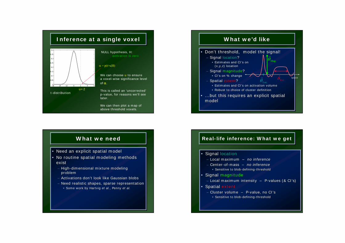
α = p(t>u|H)
NULL hypothesis, H: activation is zero
u=2t-distribution
We can choose u to ensurea voxel-wise significance level of α.
This is called an ‘uncorrected’p-value, for reasons we’ll see later.
We can then plot a map of above threshold voxels.
• Don’t threshold, model the signal!– Signal location?
• Estimates and CI’s on(x,y,z) location
– Signal magnitude?• CI’s on % change
– Spatial extent?• Estimates and CI’s on activation volume• Robust to choice of cluster definition
• ...but this requires an explicit spatial model
•• DonDon’’t threshold, model the signal!t threshold, model the signal!–– Signal Signal locationlocation??
•• Estimates and CIEstimates and CI’’s ons on((x,y,zx,y,z) location) location
–– Signal Signal magnitudemagnitude??•• CICI’’s on % changes on % change
–– Spatial Spatial extentextent??•• Estimates and CIEstimates and CI’’s on activation volumes on activation volume•• Robust to choice of cluster definitionRobust to choice of cluster definition
•• ...but this requires an explicit spatial ...but this requires an explicit spatial modelmodel
What we’d likeWhat weWhat we’’d liked like
space
Loc.θ Ext.θ
Mag.θ
What we needWhat we needWhat we need
• Need an explicit spatial model• No routine spatial modeling methods
exist– High-dimensional mixture modeling
problem– Activations don’t look like Gaussian blobs– Need realistic shapes, sparse representation
• Some work by Hartvig et al., Penny et al.
•• Need an explicit spatial modelNeed an explicit spatial model•• No routine spatial modeling methods No routine spatial modeling methods
existexist–– HighHigh--dimensional mixture modeling dimensional mixture modeling
problemproblem–– Activations donActivations don’’t look like Gaussian blobst look like Gaussian blobs–– Need realistic shapes, sparse representationNeed realistic shapes, sparse representation
•• Some work by Some work by HartvigHartvig et al.et al., Penny , Penny et al.et al.
Real-life inference: What we getRealReal--life inference: What we getlife inference: What we get
• Signal location– Local maximum – no inference– Center-of-mass – no inference
• Sensitive to blob-defining-threshold
• Signal magnitude– Local maximum intensity – P-values (& CI’s)
• Spatial extent– Cluster volume – P-value, no CI’s
• Sensitive to blob-defining-threshold
•• Signal Signal locationlocation–– Local maximum Local maximum –– no inferenceno inference–– CenterCenter--ofof--mass mass –– no inferenceno inference
•• Sensitive to blobSensitive to blob--definingdefining--thresholdthreshold
•• Signal Signal magnitudemagnitude–– Local maximum intensity Local maximum intensity –– PP--values (& CIvalues (& CI’’s)s)
•• Spatial Spatial extentextent–– Cluster volume Cluster volume –– PP--value, no CIvalue, no CI’’ss
•• Sensitive to blobSensitive to blob--definingdefining--thresholdthreshold
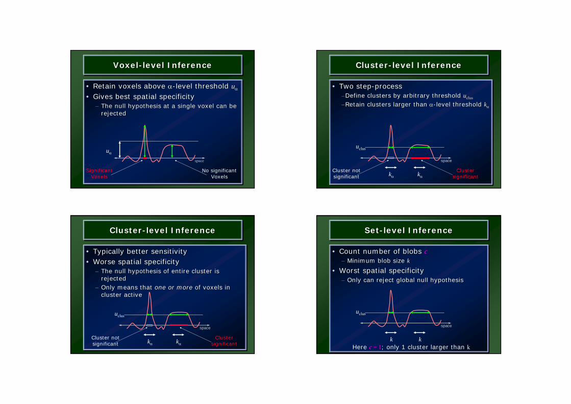
Voxel-level InferenceVoxelVoxel--level Inferencelevel Inference
• Retain voxels above α-level threshold uα
• Gives best spatial specificity– The null hypothesis at a single voxel can be
rejected
•• Retain voxels above Retain voxels above αα--level threshold level threshold uuαα
•• Gives best spatial specificityGives best spatial specificity–– The null hypothesis at a single voxel can be The null hypothesis at a single voxel can be
rejectedrejected
Significant Voxels
space
uα
No significant Voxels
Cluster-level InferenceClusterCluster--level Inferencelevel Inference
• Two step-process–Define clusters by arbitrary threshold uclus
–Retain clusters larger than α-level threshold kα
•• Two stepTwo step--processprocess––Define clusters by arbitrary threshold Define clusters by arbitrary threshold uuclusclus
––Retain clusters larger than Retain clusters larger than αα--level threshold level threshold kkαα
Cluster not significant
uclus
space
Cluster significantkα kα
Cluster-level InferenceClusterCluster--level Inferencelevel Inference
• Typically better sensitivity• Worse spatial specificity
– The null hypothesis of entire cluster is rejected
– Only means that one or more of voxels in cluster active
•• Typically better sensitivityTypically better sensitivity•• Worse spatial specificityWorse spatial specificity
–– The null hypothesis of entire cluster is The null hypothesis of entire cluster is rejectedrejected
–– Only means that Only means that one or moreone or more of voxels in of voxels in cluster activecluster active
Cluster not significant
uclus
space
Cluster significantkα kα
Set-level InferenceSetSet--level Inferencelevel Inference
• Count number of blobs c– Minimum blob size k
• Worst spatial specificity– Only can reject global null hypothesis
•• Count number of blobs Count number of blobs cc–– Minimum blob size Minimum blob size kk
•• Worst spatial specificityWorst spatial specificity–– Only can reject global null hypothesisOnly can reject global null hypothesis
uclus
space
Here c = 1; only 1 cluster larger than kk k
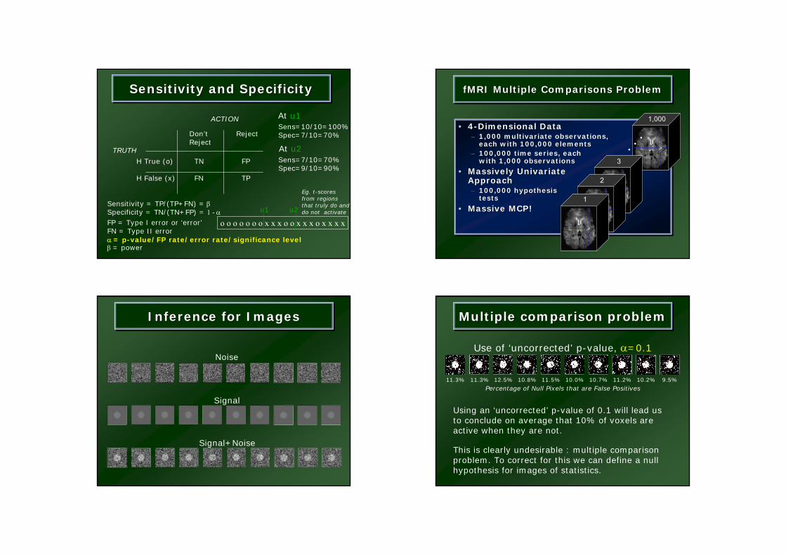
Sensitivity and SpecificitySensitivity and SpecificitySensitivity and Specificity
H True (o) TN FP
H False (x) FN TP
Don’tReject
Reject
ACTION
TRUTH
Sens=10/10=100%Spec=7/10=70%
At u1
o o o o o o o x x x o o x x x o x x x xu1 u2
Eg. t-scoresfrom regionsthat truly do and do not activate
Sens=7/10=70%Spec=9/10=90%
At u2
Sensitivity = TP/(TP+FN) = β Specificity = TN/(TN+FP) = 1 - αFP = Type I error or ‘error’FN = Type II errorα = p-value/FP rate/error rate/significance levelβ = power
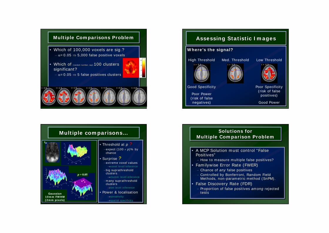
fMRI Multiple Comparisons ProblemfMRI Multiple Comparisons ProblemfMRI Multiple Comparisons Problem
• 4-Dimensional Data– 1,000 multivariate observations,
each with 100,000 elements– 100,000 time series, each
with 1,000 observations
• Massively UnivariateApproach– 100,000 hypothesis
tests
• Massive MCP!
•• 44--Dimensional DataDimensional Data–– 1,000 multivariate observations,1,000 multivariate observations,
each with 100,000 elementseach with 100,000 elements–– 100,000 time series, each 100,000 time series, each
with 1,000 observationswith 1,000 observations
•• Massively UnivariateMassively UnivariateApproachApproach–– 100,000 hypothesis100,000 hypothesis
teststests
•• Massive MCP!Massive MCP!
1,000
1
2
3. .
.
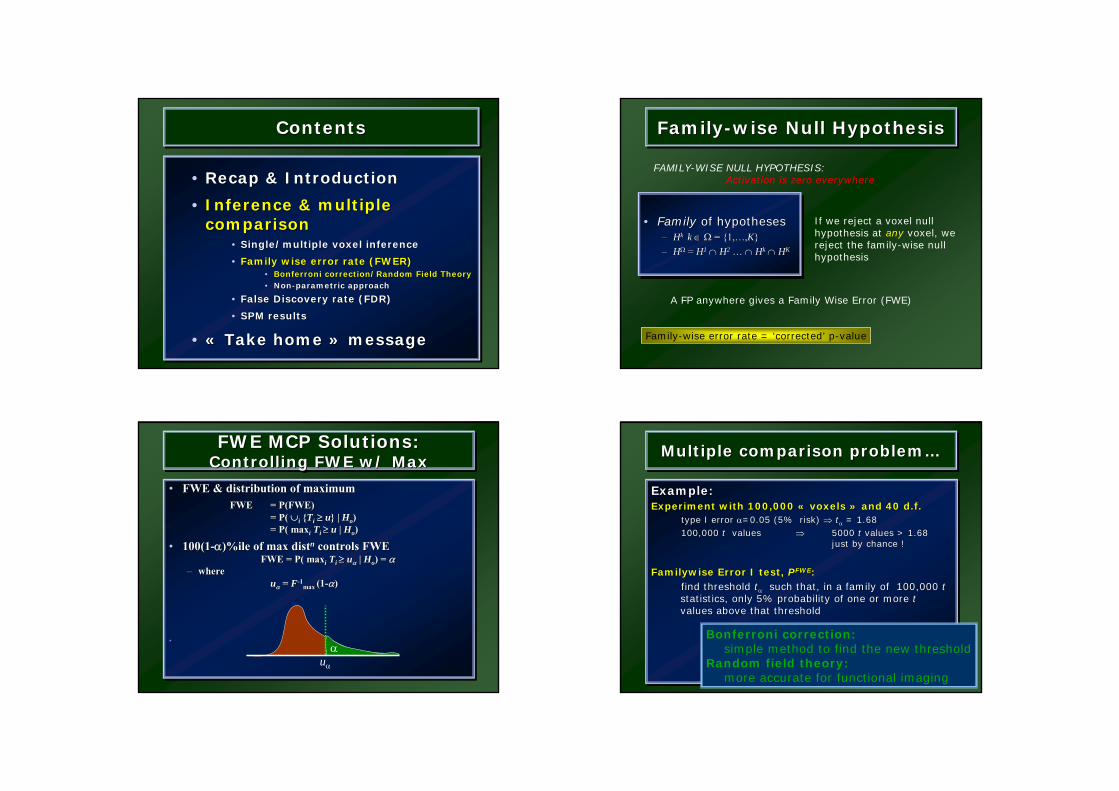
Inference for ImagesInference for ImagesInference for Images
Signal
Signal+Noise
Noise
11.3% 11.3% 12.5% 10.8% 11.5% 10.0% 10.7% 11.2% 10.2% 9.5%
Use of ‘uncorrected’ p-value, α=0.1
Percentage of Null Pixels that are False Positives
Using an ‘uncorrected’ p-value of 0.1 will lead us to conclude on average that 10% of voxels are active when they are not.
This is clearly undesirable : multiple comparison problem. To correct for this we can define a null hypothesis for images of statistics.
Multiple comparison problemMultiple comparison problemMultiple comparison problem
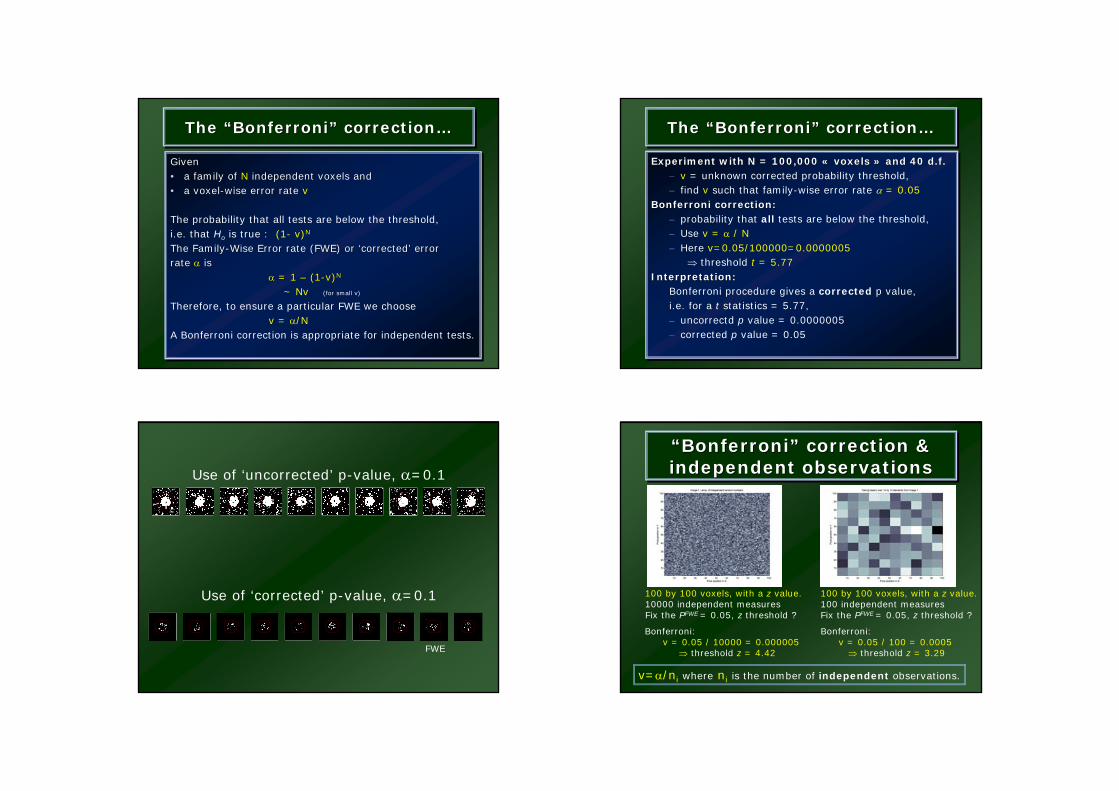
Multiple Comparisons ProblemMultiple Comparisons ProblemMultiple Comparisons Problem
• Which of 100,000 voxels are sig.?– α=0.05 ⇒ 5,000 false positive voxels
• Which of (random number, say) 100 clusters significant?– α=0.05 ⇒ 5 false positives clusters
•• Which of 100,000 voxels are sig.?Which of 100,000 voxels are sig.?–– αα=0.05 =0.05 ⇒⇒ 5,000 false positive voxels5,000 false positive voxels
•• Which ofWhich of (random number, say) (random number, say) 100 clusters 100 clusters significant?significant?–– αα=0.05 =0.05 ⇒⇒ 5 false positives clusters5 false positives clusters
t > 0.5 t > 1.5 t > 2.5 t > 3.5 t > 4.5 t > 5.5 t > 6.5
Assessing Statistic ImagesAssessing Statistic ImagesAssessing Statistic Images
Where’s the signal?WhereWhere’’s the signal?s the signal?
t > 0.5t > 3.5t > 5.5
High Threshold Med. Threshold Low Threshold
Good Specificity
Poor Power(risk of false negatives)
Poor Specificity(risk of false
positives)
Good Power
Multiple comparisons…Multiple comparisonsMultiple comparisons……
t59
Gaussian10mm FWHM(2mm pixels)
p = 0.05
• Threshold at p ?– expect (100 × p)% by chance
• Surprise ?– extreme voxel values
→voxel level inference– big suprathresholdclusters
→cluster level inference– many suprathresholdclusters
→set level inference
• Power & localisation→sensitivity→spatial specificity
•• Threshold at Threshold at p p ??–– expect (100 expect (100 ×× pp)% by )% by chancechance
•• Surprise Surprise ??–– extreme voxel valuesextreme voxel values
→→voxel level inferencevoxel level inference–– big big suprathresholdsuprathresholdclustersclusters
→→cluster level inferencecluster level inference–– many many suprathresholdsuprathresholdclustersclusters
→→set level inferenceset level inference
•• Power & localisationPower & localisation→→sensitivitysensitivity→→spatial specificityspatial specificity
Solutions forMultiple Comparison Problem
Solutions forSolutions forMultiple Comparison ProblemMultiple Comparison Problem
• A MCP Solution must control “False Positives”– How to measure multiple false positives?
• Familywise Error Rate (FWER)– Chance of any false positives– Controlled by Bonferroni, Random Field
Methods, non-parametric method (SnPM).
• False Discovery Rate (FDR)– Proportion of false positives among rejected
tests
•• A MCP Solution must control A MCP Solution must control ““False False PositivesPositives””–– How to measure multiple false positives?How to measure multiple false positives?
•• Familywise Error Rate (FWER)Familywise Error Rate (FWER)–– Chance of Chance of anyany false positivesfalse positives–– Controlled by Controlled by BonferroniBonferroni, Random Field , Random Field
Methods, nonMethods, non--parametric method (parametric method (SnPMSnPM).).
•• False Discovery Rate (FDR)False Discovery Rate (FDR)–– Proportion of false positives Proportion of false positives amongamong rejected rejected
teststests
ContentsContentsContents
• Recap & Introduction
• Inference & multiple comparison
• Single/multiple voxel inference
• Family wise error rate (FWER)• Bonferroni correction/Random Field Theory• Non-parametric approach
• False Discovery rate (FDR)
• SPM results
• « Take home » message
•• RecapRecap & Introduction& Introduction
•• InferenceInference & multiple & multiple comparisoncomparison
•• Single/multiple voxel Single/multiple voxel inferenceinference
•• FamilyFamily wisewise errorerror rate (FWER)rate (FWER)•• BonferroniBonferroni correction/correction/RandomRandom Field Field TheoryTheory•• NonNon--parametricparametric approachapproach
•• False False DiscoveryDiscovery rate (FDR)rate (FDR)
•• SPM SPM resultsresults
•• «« TakeTake homehome »» messagemessage
• Family of hypotheses– Hk k ∈ Ω = 1,…,K– HΩ = H1 ∩ H2 … ∩ Hk ∩ HK
•• FamilyFamily of hypothesesof hypotheses–– HHkk kk ∈∈ ΩΩ = 1,= 1,……,,KK–– HHΩΩ = = HH11 ∩∩ HH22 …… ∩∩ HHkk ∩∩ HHKK
Family-wise Null HypothesisFamilyFamily--wise Null Hypothesiswise Null Hypothesis
FAMILY-WISE NULL HYPOTHESIS:Activation is zero everywhere
If we reject a voxel null hypothesis at any voxel, we reject the family-wise null hypothesis
A FP anywhere gives a Family Wise Error (FWE)
Family-wise error rate = ‘corrected’ p-value
FWE MCP Solutions: Controlling FWE w/ MaxFWE MCP Solutions: FWE MCP Solutions:
Controlling FWE w/ MaxControlling FWE w/ Max
• FWE & distribution of maximumFWE = P(FWE)
= P( ∪i Ti ≥ u | Ho)= P( maxi Ti ≥ u | Ho)
• 100(1-α)%ile of max distn controls FWEFWE = P( maxi Ti ≥ uα | Ho) = α
– whereuα = F-1
max (1-α)
.
•• FWE & distribution of maximumFWE & distribution of maximumFWEFWE = P(FWE)= P(FWE)
= P( = P( ∪∪ii TTii ≥≥ uu | | HHoo))= P( max= P( maxii TTi i ≥≥ uu | | HHoo))
•• 100(1100(1--αα)%ile of )%ile of max max distdistnn controls FWEcontrols FWEFWE = P( maxFWE = P( maxii TTi i ≥≥ uuαα | | HHoo) ) = = αα
–– wherewhereuuαα = = FF--11
max max (1(1--αα))
..
uα
α
Example: Experiment with 100,000 « voxels » and 40 d.f.
type I error α=0.05 (5% risk) ⇒ tα = 1.68100,000 t values ⇒ 5000 t values > 1.68
just by chance !
Familywise Error I test, PFWE:find threshold tα such that, in a family of 100,000 tstatistics, only 5% probability of one or more tvalues above that threshold
ExampleExample: : ExperimentExperiment withwith 100,000 100,000 «« voxelsvoxels »» and 40 d.f.and 40 d.f.
type I type I errorerror αα=0.05 (5% =0.05 (5% riskrisk) ) ⇒⇒ ttαα = 1.68= 1.68100,000 100,000 t t values values ⇒⇒ 5000 5000 tt values > 1.68values > 1.68
justjust by chance !by chance !
FamilywiseFamilywise ErrorError I test, I test, PPFWEFWE::findfind thresholdthreshold ttαα suchsuch thatthat, in a , in a familyfamily of 100,000 of 100,000 ttstatisticsstatistics, , onlyonly 5% 5% probabilityprobability of one or more of one or more ttvalues values aboveabove thatthat thresholdthreshold
Multiple comparison problem…Multiple comparison problemMultiple comparison problem……
Bonferroni correction:simple method to find the new threshold
Random field theory:more accurate for functional imaging
Given • a family of N independent voxels and • a voxel-wise error rate v
The probability that all tests are below the threshold, i.e. that Ho is true : (1- v)N
The Family-Wise Error rate (FWE) or ‘corrected’ errorrate α is
α = 1 – (1-v)N
~ Nv (for small v)
Therefore, to ensure a particular FWE we choosev = α/N
A Bonferroni correction is appropriate for independent tests.
Given Given •• a family of a family of NN independent voxels and independent voxels and •• a voxela voxel--wise error rate wise error rate v
The probability that all tests are below the threshold, i.e. that Ho is true : (1- v)N
The FamilyThe Family--Wise Error rate (FWE) or Wise Error rate (FWE) or ‘‘correctedcorrected’’ errorerrorrate rate αα isis
αα = 1 = 1 –– (1(1--v)v)NN
~ Nv (for small v)
Therefore, to ensure a particular FWE we choosev = α/N
A Bonferroni correction is appropriate for independent tests.
The “Bonferroni” correction…The The ““BonferroniBonferroni”” correctioncorrection……
Experiment with N = 100,000 « voxels » and 40 d.f.– v = unknown corrected probability threshold, – find v such that family-wise error rate α = 0.05
Bonferroni correction:– probability that all tests are below the threshold,– Use v = α / N– Here v=0.05/100000=0.0000005
⇒ threshold t = 5.77Interpretation:
Bonferroni procedure gives a corrected p value, i.e. for a t statistics = 5.77, – uncorrectd p value = 0.0000005– corrected p value = 0.05
ExperimentExperiment withwith N = 100,000 N = 100,000 «« voxelsvoxels »» and 40 d.f.and 40 d.f.– v = unknown corrected probability threshold, – find v such that family-wise error rate α = 0.05
BonferroniBonferroni correction:correction:– probability that all tests are below the threshold,– Use v = α / N– Here v=0.05/100000=0.0000005
⇒ threshold t = 5.77InterpretationInterpretation::
Bonferroni procedure gives a corrected p value, i.e. for a t statistics = 5.77, – uncorrectd p value = 0.0000005– corrected p value = 0.05
The “Bonferroni” correction…The The ““BonferroniBonferroni”” correctioncorrection……
Use of ‘uncorrected’ p-value, α=0.1
FWE
Use of ‘corrected’ p-value, α=0.1
“Bonferroni” correction & independent observations““BonferroniBonferroni”” correction & correction & independent observationsindependent observations
100 by 100 voxels, with a z value.10000 independent measuresFix the PFWE = 0.05, z threshold ?
100 by 100 voxels, with a z value.100 independent measuresFix the PFWE = 0.05, z threshold ?
v=α/ni where ni is the number of independent observations.
Bonferroni: v = 0.05 / 10000 = 0.000005
⇒ threshold z = 4.42
Bonferroni: v = 0.05 / 100 = 0.0005
⇒ threshold z = 3.29
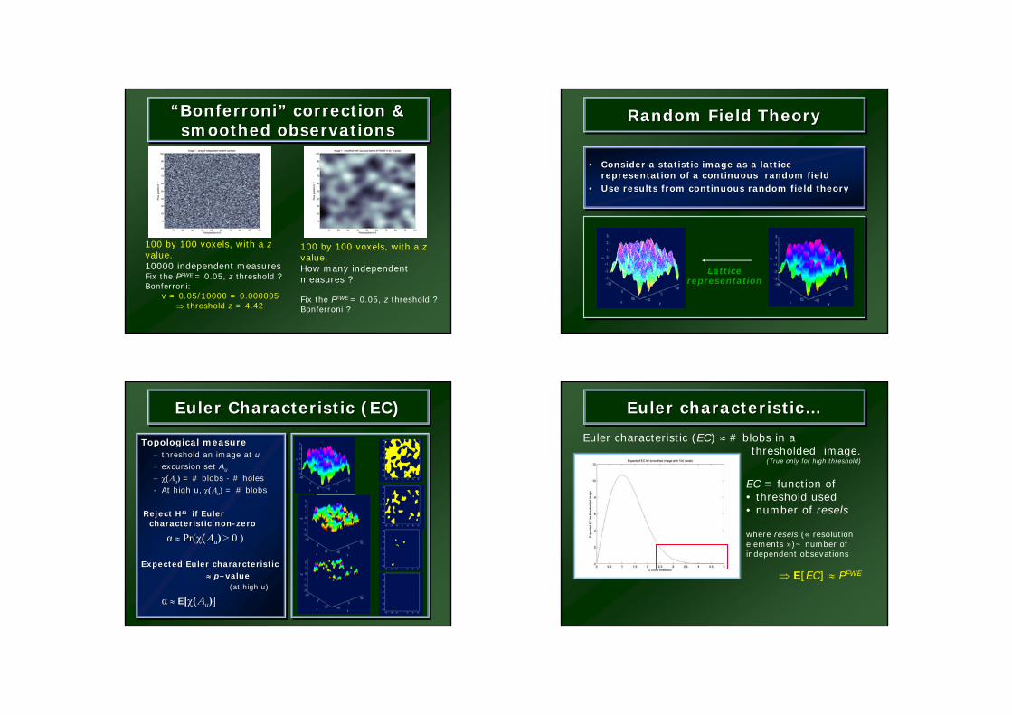
“Bonferroni” correction & smoothed observations
““BonferroniBonferroni”” correction & correction & smoothed observationssmoothed observations
100 by 100 voxels, with a zvalue.10000 independent measuresFix the PFWE = 0.05, z threshold ?Bonferroni:
v = 0.05/10000 = 0.000005 ⇒ threshold z = 4.42
100 by 100 voxels, with a zvalue.How many independentmeasures ?
Fix the PFWE = 0.05, z threshold ?Bonferroni ?
Random Field TheoryRandom Field TheoryRandom Field Theory
• Consider a statistic image as a lattice representation of a continuous random field
• Use results from continuous random field theory
•• Consider a statistic image as a lattice Consider a statistic image as a lattice representation of a continuous random fieldrepresentation of a continuous random field
•• Use results from continuous random field theoryUse results from continuous random field theory
Latticerepresentation
Euler Characteristic (EC)Euler Characteristic (EC)Euler Characteristic (EC)
Topological measure– threshold an image at u– excursion set Au
− χ(Αu) = # blobs - # holes- At high u, χ(Αu) = # blobs
Reject HΩ if Euler characteristic non-zero
α ≈ Pr(χ(Αu) > 0 )
Expected Euler chararcteristic≈ p–value
(at high u)
α ≈ E[χ(Αu)]
Topological measureTopological measure–– threshold an image at threshold an image at uu–– excursion set excursion set Auu
−− χχ(ΑΑuu) == # blobs # blobs -- # holes# holes-- At high u,At high u, χχ(ΑΑuu) == # blobs# blobs
Reject HReject HΩΩ if if Euler Euler characteristic noncharacteristic non--zerozero
αα ≈≈ Pr(Pr(χχ(ΑΑuu) > 0 ) > 0 )
Expected Euler Expected Euler chararcteristicchararcteristic≈≈ pp––valuevalue
(at high u)(at high u)
αα ≈≈ EE[[χχ(ΑΑuu)]]
Euler characteristic…Euler characteristicEuler characteristic……
Euler characteristic (EC) ≈ # blobs in athresholded image.
(True only for high threshold)
EC = function of • threshold used• number of resels
where resels (« resolutionelements »)~ number of independent obsevations
⇒ E[EC] ≈ PFWE
Euler characteristic…Euler characteristicEuler characteristic……
Threshold z-mapat 2.75
EC = 1
Threshold z-mapat 2.50
EC = 3
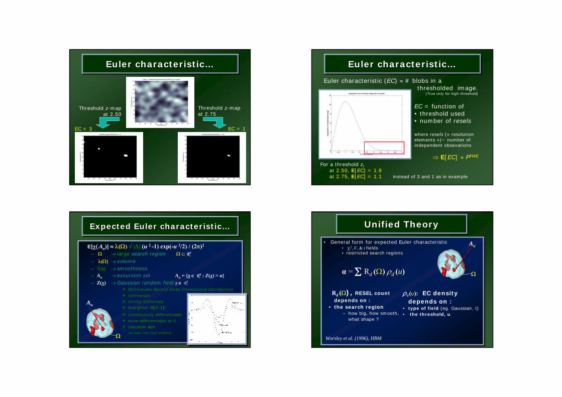
Euler characteristic…Euler characteristicEuler characteristic……
Euler characteristic (EC) ≈ # blobs in athresholded image.
(True only for high threshold)
For a threshold ztat 2.50, E[EC] = 1.9at 2.75, E[EC] = 1.1 instead of 3 and 1 as in example
EC = function of • threshold used• number of resels
where resels (« resolutionelements »)~ number of independent obsevations
⇒ E[EC] ≈ PFWE
E[χ(Αu)] ≈ λ(Ω) √ |Λ| (u 2 -1) exp(-u 2/2) / (2π)2
– Ω → large search region Ω ⊂ R3
– λ(Ω) → volume– √|Λ| → smoothness– Au → excursion set Au = x ∈ R3 : Z(x) > u– Z(x) → Gaussian random field x ∈ R3
+ Multivariate Normal Finite Dimensional distributions+ continuous+ strictly stationary+ marginal N(0,1)
+ continuously differentiable
+ twice differentiable at 0+ Gaussian ACF
(at least near local maxima)
EE[[χχ(ΑΑuu)] ] ≈≈ λλ((ΩΩ)) √√ ||ΛΛ|| (u u 2 2 --11) expexp(--u u 22/2/2) / (22ππ)22
–– ΩΩ →→ largelarge search regionsearch region ΩΩ ⊂⊂ RR3 3
–– λλ((Ω)Ω) →→ volumevolume–– √√||ΛΛ|| →→ smoothnesssmoothness–– AAuu →→ excursion setexcursion set AAuu = x ∈ RR33 : Z(x) > u– Z(x) →→ Gaussian Gaussian random fieldrandom field x ∈ RR33
+ + Multivariate Normal Finite Dimensional distributionsMultivariate Normal Finite Dimensional distributions
+ + continuouscontinuous
+ + strictly stationarystrictly stationary
+ + marginal Nmarginal N((0,10,1))
++ continuously differentiablecontinuously differentiable
++ twice differentiable at 0twice differentiable at 0
++ Gaussian Gaussian ACFACF
(at least near local maxima)(at least near local maxima)
Expected Euler characteristic…Expected Euler characteristicExpected Euler characteristic……
Au
Ω
• General form for expected Euler characteristic• χ2, F, & t fields • restricted search regions
α = Σ Rd (Ω) ρd (u)
•• General form for expected Euler characteristicGeneral form for expected Euler characteristic•• χχ22, , FF, & , & tt fields fields •• restricted search regionsrestricted search regions
αα = = ΣΣ RRd d ((ΩΩ)) ρρd d ((uu))
Unified TheoryUnified TheoryUnified Theory
Rd (Ω), RESEL count depends on :
• the search region– how big, how smooth,
what shape ?
ρd (υ): EC density depends on :
• type of field (eg. Gaussian, t)• the threshold, u.
Worsley et al. (1996), HBM
Au
Ω
• General form for expected Euler characteristic• χ2, F, & t fields • restricted search regions
α = Σ Rd (Ω) ρd (u)
•• General form for expected Euler characteristicGeneral form for expected Euler characteristic•• χχ22, , FF, & , & tt fields fields •• restricted search regionsrestricted search regions
αα = = ΣΣ RRd d ((ΩΩ)) ρρd d ((uu))
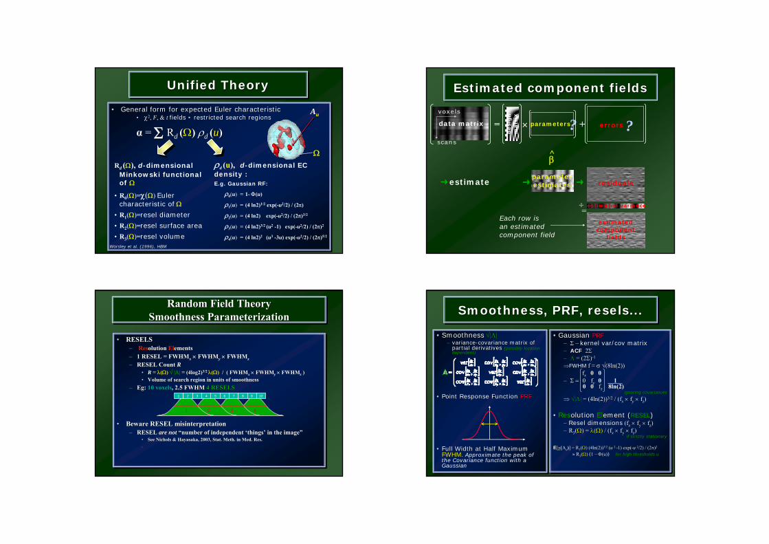
Unified TheoryUnified TheoryUnified Theory
Rd (Ω), d-dimensional Minkowski functional of Ω
• R0(Ω)=χ(Ω) Euler characteristic of Ω
• R1(Ω)=resel diameter
• R2(Ω)=resel surface area
• R3(Ω)=resel volume
ρd (u), d-dimensional EC density :E.g. Gaussian RF:
ρ0(u) = 1- Φ(u)
ρ1(u) = (4 ln2)1/2 exp(-u2/2) / (2π)
ρ2(u) = (4 ln2) exp(-u2/2) / (2π)3/2
ρ3(u) = (4 ln2)3/2 (u2 -1) exp(-u2/2) / (2π)2
ρ4(u) = (4 ln2)2 (u3 -3u) exp(-u2/2) / (2π)5/2
Au
Ω
Worsley et al. (1996), HBM
Estimated component fieldsEstimated component fieldsEstimated component fields
data matrix
desi
gn
m
atr
ix
parameters errors+ ?= × ?voxelsvoxels
scansscans
estimate
β
residuals
estimatedcomponent
fields
parameterestimates
estimated variance÷=
Each row isan estimatedcomponent field
• RESELS– Resolution Elements– 1 RESEL = FWHMx × FWHMy × FWHMz– RESEL Count R
• R = λ(Ω) √ |Λ| = (4log2)3/2 λ(Ω) / ( FWHMx × FWHMy × FWHMz ) • Volume of search region in units of smoothness
– Eg: 10 voxels, 2.5 FWHM 4 RESELS
• Beware RESEL misinterpretation– RESEL are not “number of independent ‘things’ in the image”
• See Nichols & Hayasaka, 2003, Stat. Meth. in Med. Res..
•• RESELSRESELS–– ResResolution olution ElElementsements–– 1 RESEL = 1 RESEL = FWHMFWHMxx × × FWHMFWHMyy × × FWHMFWHMzz–– RESEL Count RESEL Count RR
•• RR = = λλ((ΩΩ)) √√ ||ΛΛ|| = (4log2)= (4log2)3/2 3/2 λλ((ΩΩ)) / ( / ( FWHMFWHMxx × × FWHMFWHMyy × × FWHMFWHMzz ) ) •• Volume of search region in units of smoothnessVolume of search region in units of smoothness
–– EgEg: : 10 voxels10 voxels, 2.5 FWHM , 2.5 FWHM 4 RESELS4 RESELS
•• Beware RESEL misinterpretationBeware RESEL misinterpretation–– RESEL RESEL are not are not ““number of independent number of independent ‘‘thingsthings’’ in the imagein the image””
•• See Nichols & Hayasaka, 2003, Stat. See Nichols & Hayasaka, 2003, Stat. MethMeth. in Med. Res.. in Med. Res...
Random Field TheorySmoothness Parameterization
Random Field TheoryRandom Field TheorySmoothness ParameterizationSmoothness Parameterization
1 2 3 4
2 4 6 8 101 3 5 7 9
[ ] [ ] [ ][ ] [ ] [ ][ ] [ ] [ ] ⎟
⎟⎟
⎠
⎞
⎜⎜⎜
⎝
⎛
=Λ
∂∂
∂∂
∂∂
∂∂
∂∂
∂∂
∂∂
∂∂
∂∂
∂∂
∂∂
∂∂
∂∂
∂∂
∂∂
ze
ze
ye
ze
xe
ze
ye
ye
ye
xe
ze
xe
ye
xe
xe
var,cov,cov,covvar,cov,cov,covvar
Smoothness, PRF, resels...Smoothness, PRF, Smoothness, PRF, reselsresels......
• Smoothness √|Λ|– variance-covariance matrix of
partial derivatives (possibly location dependent)
• Point Response Function PRF
• Full Width at Half Maximum FWHM. Approximate the peak of the Covariance function with a Gaussian
•• SmoothnessSmoothness √√||ΛΛ||–– variancevariance--covariance matrix of covariance matrix of
partial derivatives partial derivatives (possibly location (possibly location dependent)dependent)
•• Point Response Function Point Response Function PRFPRF
•• Full Width at Half Maximum Full Width at Half Maximum FWHM.FWHM. Approximate the peak of the Covariance function with a Gaussian
• Gaussian PRF– Σ – kernel var/cov matrix– ACF 2Σ– Λ = (2Σ)-1
⇒FWHM f = σ √(8ln(2))fx 0 0
– Σ = 0 fy 0 10 0 fz 8ln(2)
ignoring covariances
⇒ √|Λ| = (4ln(2))3/2 / (fx × fy × fz)
• Resolution Element (RESEL)– Resel dimensions (fx × fy × fz)– R3(Ω) = λ(Ω) / (fx × fy × fz)
if strictly stationary
E[χ(Αu)] = R3(Ω) (4ln(2))3/2 (u 2 -1) exp(-u 2/2) / (2π)2
≈ R3(Ω) (1 – Φ(u)) for high thresholds u
•• Gaussian Gaussian PRFPRF–– ΣΣ –– kernel kernel var/covvar/cov matrixmatrix–– ACFACF 22ΣΣ–– ΛΛ = (2= (2ΣΣ))--11
⇒⇒FWHMFWHM f = f = σσ √√(8ln(2))(8ln(2))ffxx 0 0
–– ΣΣ = = 00 ffyy 0 10 0 ffzz 8ln(2)
ignoring ignoring covariancescovariances
⇒⇒ √√||ΛΛ|| = (4ln(2))= (4ln(2))3/23/2 / (/ (ffxx ×× ffyy ×× ffzz))
•• ResResolution olution ElElement (ement (RESELRESEL))–– ReselResel dimensionsdimensions ((ffxx ×× ffyy ×× ffzz))–– RR33((ΩΩ) = ) = λλ((ΩΩ)) / (/ (ffxx ×× ffyy ×× ffzz))
if strictly stationaryif strictly stationary
EE[[χχ(ΑΑuu)]] = R= R33((ΩΩ) (4ln(2))) (4ln(2))3/23/2 ((u u 2 2 --1) exp(1) exp(--u u 22/2) / (2/2) / (2ππ))22
≈≈ RR33((ΩΩ) ) ((1 1 –– ΦΦ(u)(u))) for high thresholds ufor high thresholds u
Λ
RFT AssumptionsRFT AssumptionsRFT Assumptions
• Model fit & assumptions– valid distributional
results
• Multivariate normality– of component images
• Covariance function of component images must be
- Can be nonstationary
- Twice differentiable
•• Model fit & assumptionsModel fit & assumptions–– valid distributional valid distributional
resultsresults
•• Multivariate normalityMultivariate normality–– of of componentcomponent imagesimages
•• Covariance function of Covariance function of componentcomponent images must images must bebe
-- Can be Can be nonstationarynonstationary
-- Twice differentiableTwice differentiable
Smoothnesssmoothness » voxel size
lattice approximationsmoothness estimation
practicallyFWHM ≥ 3 × VoxDim
otherwiseconservative
“Typical” applied smoothing:Single Subj fMRI: 6mm
PET: 12mmMulti Subj fMRI: 8-12mm
PET: 16mm
Level of smoothing should actually depend on what
you’re looking for…
SmoothnessSmoothnesssmoothness smoothness »» voxel sizevoxel size
lattice approximationlattice approximationsmoothness estimationsmoothness estimation
practicallypracticallyFWHMFWHM ≥≥ 3 3 ×× VoxDimVoxDim
otherwiseotherwiseconservativeconservative
““TypicalTypical”” applied smoothing:applied smoothing:Single Single SubjSubj fMRI: 6mmfMRI: 6mm
PET: 12mmPET: 12mmMulti Multi SubjSubj fMRI: 8fMRI: 8--12mm12mm
PET: 16mm PET: 16mm
Level of smoothing should Level of smoothing should actually depend on what actually depend on what
youyou’’re looking forre looking for……
Random Field IntuitionRandom Field IntuitionRandom Field Intuition
• Corrected P-value for voxel value tPc = P(max T > t)
≈ E(χt)≈ λ(Ω) |Λ|1/2 t2 exp(-t2/2)
• Statistic value t increases– Pc decreases (but only for large t)
• Search volume increases (bigger Ω)
– Pc increases (more severe MCP)• Smoothness increases (roughness |Λ|1/2 decreases)
– Pc decreases (less severe MCP)
•• Corrected PCorrected P--value for voxel value value for voxel value ttPPcc = = P(maxP(max TT > > tt))
≈≈ E(E(χχtt))≈≈ λλ((ΩΩ) |) |ΛΛ||1/21/2 tt2 2 exp(exp(--tt22/2)/2)
•• Statistic value Statistic value tt increasesincreases–– PPcc decreases (but only for large decreases (but only for large tt))
•• Search volume increases Search volume increases (bigger (bigger ΩΩ))
–– PPcc increases (more severe MCP)increases (more severe MCP)•• Smoothness increases Smoothness increases (roughness (roughness ||ΛΛ||1/21/2 decreases)decreases)
–– PPcc decreases (less severe MCP)decreases (less severe MCP)
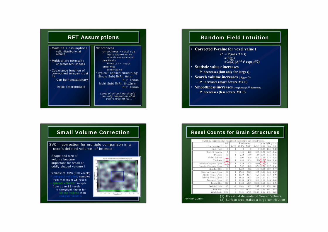
Small Volume CorrectionSmall Volume CorrectionSmall Volume Correction
SVC = correction for multiple comparison in a user’s defined volume ‘of interest’.
SVC = correction for multiple comparison in a SVC = correction for multiple comparison in a useruser’’s defined volume s defined volume ‘‘of interestof interest’’..
Shape and size of volume becomeimportant for small or oddly shaped volume !
Example of SVC (900 voxels)• compact volume: samples
from maximum 16 resels• spread volume: sample
from up to 36 resels⇒ threshold higher for
spread volume thancompact volume.
Resel Counts for Brain StructuresReselResel Counts for Brain StructuresCounts for Brain Structures
FWHM=20mm(1) Threshold depends on Search Volume(2) Surface area makes a large contribution

SummarySummarySummary
• We should correct for multiple comparisons– We can use Random Field Theory (RFT) or other methods
• RFT requires– a good lattice approximation to underlying multivariate
Gaussian fields,
– that these fields are continuous with a twice differentiable correlation function
• To a first approximation, RFT is a Bonferroni correction using RESELS.
• We only need to correct for the volume of interest.
• Depending on nature of signal we can trade-off anatomical specificity for signal sensitivity with the use of cluster-level inference.
ContentsContentsContents
• Recap & Introduction
• Inference & multiple comparison
• Single/multiple voxel inference
• Family wise error rate (FWER)• Bonferroni correction/Random Field Theory• Non-parametric approach
• False Discovery rate (FDR)
• SPM results
• « Take home » message
•• RecapRecap & Introduction& Introduction
•• InferenceInference & multiple & multiple comparisoncomparison
•• Single/multiple voxel Single/multiple voxel inferenceinference
•• FamilyFamily wisewise errorerror rate (FWER)rate (FWER)•• BonferroniBonferroni correction/correction/RandomRandom Field Field TheoryTheory•• NonNon--parametricparametric approachapproach
•• False False DiscoveryDiscovery rate (FDR)rate (FDR)
•• SPM SPM resultsresults
•• «« TakeTake homehome »» messagemessage
NonparametricPermutation TestNonparametric
Permutation Test
• Parametric methods– Assume distribution of
statistic under nullhypothesis
• Nonparametric methods– Use data to find
distribution of statisticunder null hypothesis
– Any statistic!
• Parametric methods– Assume distribution of
statistic under nullhypothesis
• Nonparametric methods– Use data to find
distribution of statisticunder null hypothesis
– Any statistic!
5%
Parametric Null Distribution
5%
Nonparametric Null Distribution
Permutation Test : Toy ExamplePermutation Test : Toy Example
• Data from V1 voxel in visual stim. experimentA: Active, flashing checkerboard B: Baseline, fixation6 blocks, ABABAB Just consider block averages...
• Null hypothesis Ho– No experimental effect, A & B labels arbitrary
• Statistic– Mean difference
• Data from V1 voxel in visual stim. experimentA: Active, flashing checkerboard B: Baseline, fixation6 blocks, ABABAB Just consider block averages...
• Null hypothesis Ho– No experimental effect, A & B labels arbitrary
• Statistic– Mean difference
96.0696.0699.7699.7687.8387.8399.9399.9390.4890.48103.00103.00
BBAABBAABBAA
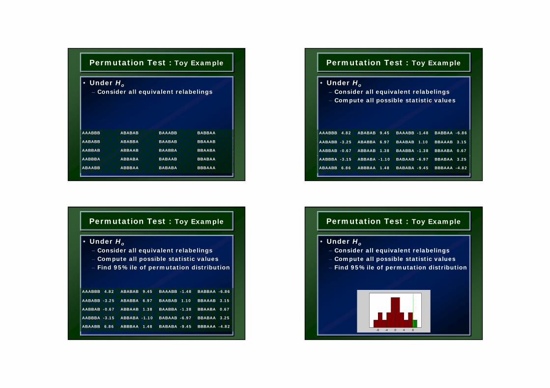
Permutation Test : Toy ExamplePermutation Test : Toy Example
• Under Ho– Consider all equivalent relabelings
•• Under Under HHoo
–– Consider all equivalent Consider all equivalent relabelingsrelabelings
BBBAAABBBAAABABABABABABAABBBAAABBBAAABAABBABAABB
BBABAABBABAABABAABBABAABABBABAABBABAAABBBAAABBBA
BBAABABBAABABAABBABAABBAABBAABABBAABAABBABAABBAB
BBAAABBBAAABBAABABBAABABABABBAABABBAAABABBAABABB
BABBAABABBAABAAABBBAAABBABABABABABABAAABBBAAABBB
Permutation Test : Toy ExamplePermutation Test : Toy Example
• Under Ho– Consider all equivalent relabelings– Compute all possible statistic values
•• Under Under HHoo
–– Consider all equivalent Consider all equivalent relabelingsrelabelings–– Compute all possible statistic valuesCompute all possible statistic values
BBBAAA BBBAAA --4.824.82BABABA BABABA --9.459.45ABBBAA 1.48ABBBAA 1.48ABAABB 6.86ABAABB 6.86
BBABAA 3.25BBABAA 3.25BABAAB BABAAB --6.976.97ABBABA ABBABA --1.101.10AABBBA AABBBA --3.153.15
BBAABA 0.67BBAABA 0.67BAABBA BAABBA --1.381.38ABBAAB 1.38ABBAAB 1.38AABBAB AABBAB --0.670.67
BBAAAB 3.15BBAAAB 3.15BAABAB 1.10BAABAB 1.10ABABBA 6.97ABABBA 6.97AABABB AABABB --3.253.25
BABBAA BABBAA --6.866.86BAAABB BAAABB --1.481.48ABABAB 9.45ABABAB 9.45AAABBB 4.82AAABBB 4.82
Permutation Test : Toy ExamplePermutation Test : Toy Example
• Under Ho– Consider all equivalent relabelings– Compute all possible statistic values– Find 95%ile of permutation distribution
•• Under Under HHoo
–– Consider all equivalent Consider all equivalent relabelingsrelabelings–– Compute all possible statistic valuesCompute all possible statistic values–– Find 95%ile of permutation distributionFind 95%ile of permutation distribution
BBBAAA BBBAAA --4.824.82BABABA BABABA --9.459.45ABBBAA 1.48ABBBAA 1.48ABAABB 6.86ABAABB 6.86
BBABAA 3.25BBABAA 3.25BABAAB BABAAB --6.976.97ABBABA ABBABA --1.101.10AABBBA AABBBA --3.153.15
BBAABA 0.67BBAABA 0.67BAABBA BAABBA --1.381.38ABBAAB 1.38ABBAAB 1.38AABBAB AABBAB --0.670.67
BBAAAB 3.15BBAAAB 3.15BAABAB 1.10BAABAB 1.10ABABBA 6.97ABABBA 6.97AABABB AABABB --3.253.25
BABBAA BABBAA --6.866.86BAAABB BAAABB --1.481.48ABABAB 9.45ABABAB 9.45AAABBB 4.82AAABBB 4.82
Permutation Test : Toy ExamplePermutation Test : Toy Example
• Under Ho– Consider all equivalent relabelings– Compute all possible statistic values– Find 95%ile of permutation distribution
• Under Ho– Consider all equivalent relabelings– Compute all possible statistic values– Find 95%ile of permutation distribution
0 4 8-4-8
Permutation Test : Toy ExamplePermutation Test : Toy Example
• Under Ho– Consider all equivalent relabelings– Compute all possible statistic values– Find 95%ile of permutation distribution
•• Under Under HHoo
–– Consider all equivalent Consider all equivalent relabelingsrelabelings–– Compute all possible statistic valuesCompute all possible statistic values–– Find 95%ile of permutation distributionFind 95%ile of permutation distribution
BBBAAA BBBAAA --4.824.82BABABA BABABA --9.459.45ABBBAA 1.48ABBBAA 1.48ABAABB 6.86ABAABB 6.86
BBABAA 3.25BBABAA 3.25BABAAB BABAAB --6.976.97ABBABA ABBABA --1.101.10AABBBA AABBBA --3.153.15
BBAABA 0.67BBAABA 0.67BAABBA BAABBA --1.381.38ABBAAB 1.38ABBAAB 1.38AABBAB AABBAB --0.670.67
BBAAAB 3.15BBAAAB 3.15BAABAB 1.10BAABAB 1.10ABABBA 6.97ABABBA 6.97AABABB AABABB --3.253.25
BABBAA BABBAA --6.866.86BAAABB BAAABB --1.481.48ABABABABABAB 9.459.45AAABBB 4.82AAABBB 4.82
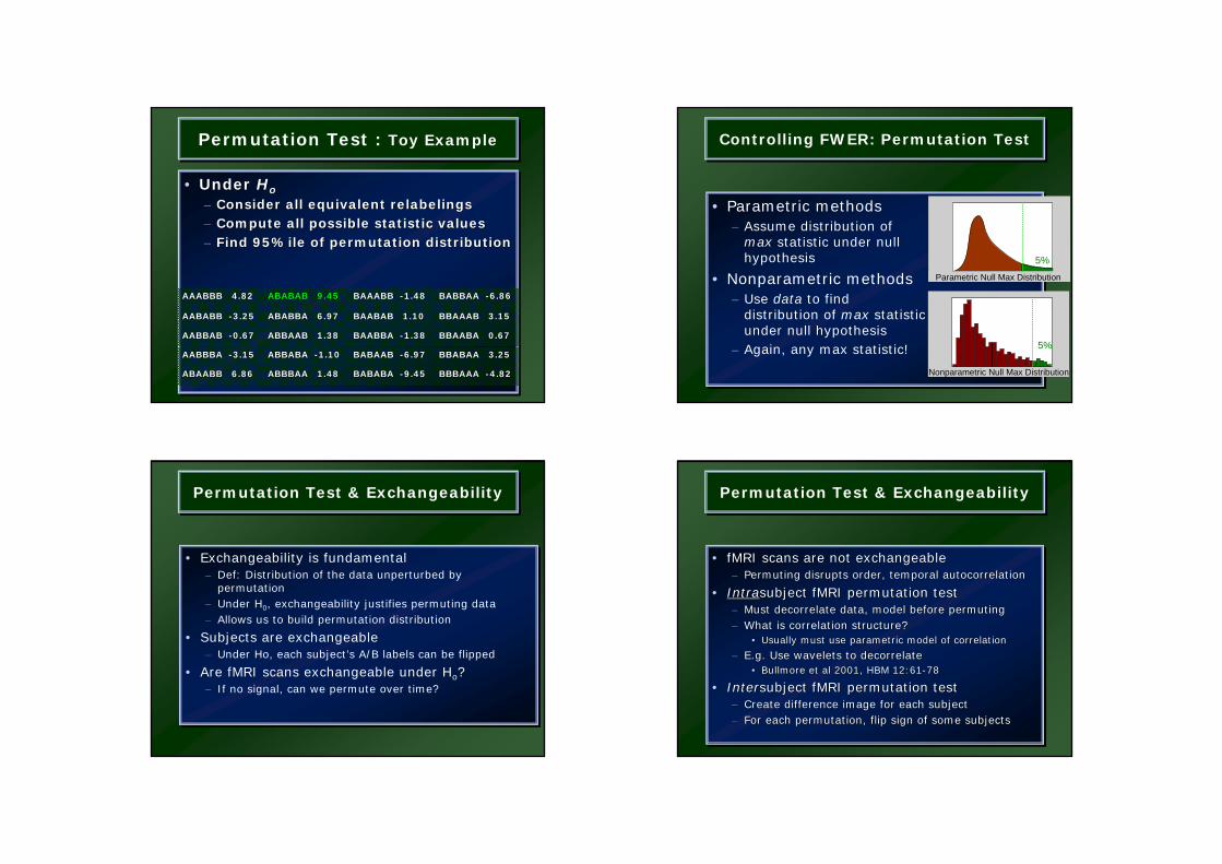
Controlling FWER: Permutation TestControlling FWER: Permutation Test
• Parametric methods– Assume distribution of
max statistic under nullhypothesis
• Nonparametric methods– Use data to find
distribution of max statisticunder null hypothesis
– Again, any max statistic!
• Parametric methods– Assume distribution of
max statistic under nullhypothesis
• Nonparametric methods– Use data to find
distribution of max statisticunder null hypothesis
– Again, any max statistic!
5%
Parametric Null Max Distribution
5%
Nonparametric Null Max Distribution
Permutation Test & ExchangeabilityPermutation Test & Exchangeability
• Exchangeability is fundamental– Def: Distribution of the data unperturbed by
permutation– Under H0, exchangeability justifies permuting data– Allows us to build permutation distribution
• Subjects are exchangeable– Under Ho, each subject’s A/B labels can be flipped
• Are fMRI scans exchangeable under Ho?– If no signal, can we permute over time?
Permutation Test & ExchangeabilityPermutation Test & Exchangeability
• fMRI scans are not exchangeable– Permuting disrupts order, temporal autocorrelation
• Intrasubject fMRI permutation test– Must decorrelate data, model before permuting– What is correlation structure?
• Usually must use parametric model of correlation
– E.g. Use wavelets to decorrelate• Bullmore et al 2001, HBM 12:61-78
• Intersubject fMRI permutation test– Create difference image for each subject– For each permutation, flip sign of some subjects
•• fMRI scans are not exchangeablefMRI scans are not exchangeable–– Permuting disrupts order, temporal autocorrelationPermuting disrupts order, temporal autocorrelation
•• IntraIntrasubject fMRI permutation testsubject fMRI permutation test–– Must decorrelate data, model before permutingMust decorrelate data, model before permuting–– What is correlation structure?What is correlation structure?
•• Usually must use parametric model of correlationUsually must use parametric model of correlation
–– E.g. Use wavelets to E.g. Use wavelets to decorrelatedecorrelate•• BullmoreBullmore et al 2001, HBM 12:61et al 2001, HBM 12:61--7878
•• InterIntersubject fMRI permutation testsubject fMRI permutation test–– Create difference image for each subjectCreate difference image for each subject–– For each permutation, flip sign of some subjectsFor each permutation, flip sign of some subjects

Permutation Test : ExamplePermutation Test : ExamplePermutation Test : Example
• fMRI Study of Working Memory – 12 subjects, block design Marshuetz et al (2000)
– Item Recognition• Active:View five letters, 2s pause,
view probe letter, respond• Baseline: View XXXXX, 2s pause,
view Y or N, respond
• Second Level RFX– Difference image, A-B constructed
for each subject– One sample, smoothed variance t test
...
D
yes
...
UBKDA
Active
...
N
no
...
XXXXX
Baseline
Permutation Test : ExamplePermutation Test : Example
• Permute!– 212 = 4,096 ways to flip 12 A/B labels– For each, note maximum of t image.
•• Permute!Permute!–– 221212 = 4,096 ways to flip 12 A/B labels= 4,096 ways to flip 12 A/B labels–– For each, note maximum of For each, note maximum of t t imageimage..
Permutation DistributionMaximum t
Maximum Intensity Projection Thresholded t
t11 Statistic, RF & Bonf. Thresholdt11 Statistic, Nonparametric Threshold
uRF = 9.87uBonf = 9.805 sig. vox.
uPerm = 7.67 58 sig. vox.
Test Level vs. t11 Threshold
•Compare with Bonferroniα = 0.05/110,776
•Compare with parametric RFT110,776 2×2×2mm voxels5.1×5.8×6.9mm FWHM
smoothness462.9 RESELs
Does this Generalize?RFT vs Bonf. vs Perm.
Does this Generalize?RFT vs Bonf. vs Perm.
t Threshold (0.05 Corrected)
df RF Bonf PermVerbal Fluency 4 4701.32 42.59 10.14Location Switching 9 11.17 9.07 5.83Task Switching 9 10.79 10.35 5.10Faces: Main Effect 11 10.43 9.07 7.92Faces: Interaction 11 10.70 9.07 8.26Item Recognition 11 9.87 9.80 7.67Visual Motion 11 11.07 8.92 8.40Emotional Pictures 12 8.48 8.41 7.15Pain: Warning 22 5.93 6.05 4.99Pain: Anticipation 22 5.87 6.05 5.05
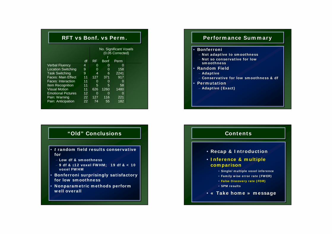
RFT vs Bonf. vs Perm.RFT vs Bonf. vs Perm.
No. Significant Voxels (0.05 Corrected)
t df RF Bonf Perm
Verbal Fluency 4 0 0 0Location Switching 9 0 0 158Task Switching 9 4 6 2241Faces: Main Effect 11 127 371 917Faces: Interaction 11 0 0 0Item Recognition 11 5 5 58Visual Motion 11 626 1260 1480Emotional Pictures 12 0 0 0Pain: Warning 22 127 116 221Pain: Anticipation 22 74 55 182
Performance SummaryPerformance SummaryPerformance Summary
• Bonferroni– Not adaptive to smoothness– Not so conservative for low
smoothness
• Random Field– Adaptive– Conservative for low smoothness & df
• Permutation– Adaptive (Exact)
•• BonferroniBonferroni–– Not adaptive to smoothnessNot adaptive to smoothness–– Not so conservative for low Not so conservative for low
smoothnesssmoothness
•• Random FieldRandom Field–– AdaptiveAdaptive–– Conservative for low smoothness & Conservative for low smoothness & dfdf
•• PermutationPermutation–– Adaptive (Exact)Adaptive (Exact)
“Old” Conclusions“Old” Conclusions
• t random field results conservative for– Low df & smoothness– 9 df & ≤12 voxel FWHM; 19 df & < 10
voxel FWHM
• Bonferroni surprisingly satisfactory for low smoothness
• Nonparametric methods perform well overall
• t random field results conservative for– Low df & smoothness– 9 df & ≤12 voxel FWHM; 19 df & < 10
voxel FWHM
• Bonferroni surprisingly satisfactory for low smoothness
• Nonparametric methods perform well overall
ContentsContentsContents
• Recap & Introduction
• Inference & multiple comparison
• Single/multiple voxel inference
• Family wise error rate (FWER)
• False Discovery rate (FDR)
• SPM results
• « Take home » message
•• RecapRecap & Introduction& Introduction
•• InferenceInference & multiple & multiple comparisoncomparison
•• Single/multiple voxel Single/multiple voxel inferenceinference
•• FamilyFamily wisewise errorerror rate (FWER)rate (FWER)
•• False False DiscoveryDiscovery rate (FDR)rate (FDR)
•• SPM SPM resultsresults
•• «« TakeTake homehome »» messagemessage
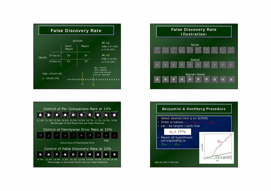
False Discovery RateFalse Discovery RateFalse Discovery Rate
H True (o) TN FP
H False (x) FN TP
Don’tReject
Reject
ACTION
TRUTH
FDR=3/17=18%α=3/10=30%
At u1
o o o o o o o x x x o o x x x o x x x x x x x x
u1 u2
Eg. t-scoresfrom regionsthat truly do and do not activate
FDR=1/12=8%α=1/10=10%
At u2
FDR = FP/(FP+TP)
α = FP/(FP+TN)
False Discovery RateIllustration:
False Discovery RateFalse Discovery RateIllustration:Illustration:
Signal
Signal+Noise
Noise
11.3% 11.3% 12.5% 10.8% 11.5% 10.0% 10.7% 11.2% 10.2% 9.5%
Control of Per Comparison Rate at 10%
Percentage of Null Pixels that are False Positives
FWE
Control of Familywise Error Rate at 10%
Occurrence of Familywise Error
6.7% 10.4% 14.9% 9.3% 16.2% 13.8% 14.0% 10.5% 12.2% 8.7%
Control of False Discovery Rate at 10%
Percentage of Activated Pixels that are False Positives
Benjamini & Hochberg ProcedureBenjaminiBenjamini & Hochberg Procedure& Hochberg Procedure
• Select desired limit q on E(FDR)• Order p-values, p(1) ≤ p(2) ≤ ... ≤ p(V)
• Let r be largest i such that
• Reject all hypotheses corresponding top(1), ... , p(r).
•• Select desired limit Select desired limit qq on E(FDR)on E(FDR)•• Order pOrder p--values, values, pp(1)(1) ≤≤ pp(2)(2) ≤≤ ... ... ≤≤ pp((VV))
•• Let Let rr be largest be largest ii such thatsuch that
•• Reject all hypotheses Reject all hypotheses corresponding tocorresponding topp(1)(1), ... , , ... , pp((rr))..
p(i) ≤ i/V*q
p(i)
i/Vi/V × q/c(V)
p-va
lue
0 1
01
JRSS-B (1995) 57:289-300
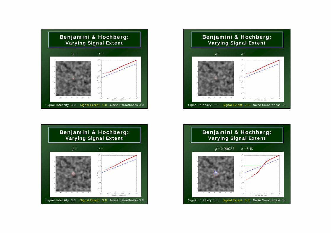
Benjamini & Hochberg:Varying Signal Extent
BenjaminiBenjamini & Hochberg:& Hochberg:Varying Signal ExtentVarying Signal Extent
Signal Intensity 3.0 Signal Extent 1.0 Noise Smoothness 3.0
p = z =
1Signal Intensity 3.0 Signal Extent 2.0 Noise Smoothness 3.0
p = z =
2
Benjamini & Hochberg:Varying Signal Extent
BenjaminiBenjamini & Hochberg:& Hochberg:Varying Signal ExtentVarying Signal Extent
Signal Intensity 3.0 Signal Extent 3.0 Noise Smoothness 3.0
p = z =
3
Benjamini & Hochberg:Varying Signal Extent
BenjaminiBenjamini & Hochberg:& Hochberg:Varying Signal ExtentVarying Signal Extent
Signal Intensity 3.0 Signal Extent 5.0 Noise Smoothness 3.0
p = 0.000252 z = 3.48
4
Benjamini & Hochberg:Varying Signal Extent
BenjaminiBenjamini & Hochberg:& Hochberg:Varying Signal ExtentVarying Signal Extent
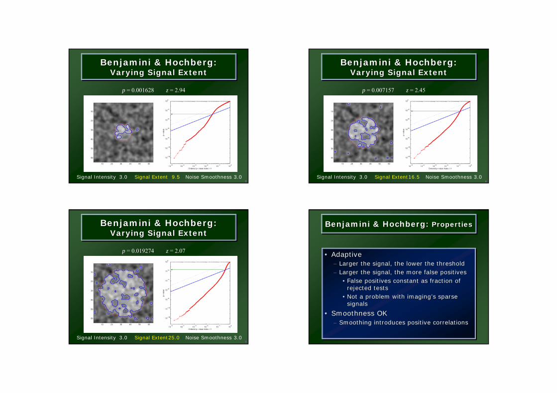
Signal Intensity 3.0 Signal Extent 9.5 Noise Smoothness 3.0
p = 0.001628 z = 2.94
5
Benjamini & Hochberg:Varying Signal Extent
BenjaminiBenjamini & Hochberg:& Hochberg:Varying Signal ExtentVarying Signal Extent
Signal Intensity 3.0 Signal Extent16.5 Noise Smoothness 3.0
p = 0.007157 z = 2.45
6
Benjamini & Hochberg:Varying Signal Extent
BenjaminiBenjamini & Hochberg:& Hochberg:Varying Signal ExtentVarying Signal Extent
Signal Intensity 3.0 Signal Extent25.0 Noise Smoothness 3.0
p = 0.019274 z = 2.07
7
Benjamini & Hochberg:Varying Signal Extent
BenjaminiBenjamini & Hochberg:& Hochberg:Varying Signal ExtentVarying Signal Extent
Benjamini & Hochberg: PropertiesBenjaminiBenjamini & Hochberg: & Hochberg: PropertiesProperties
• Adaptive– Larger the signal, the lower the threshold– Larger the signal, the more false positives
• False positives constant as fraction of rejected tests
• Not a problem with imaging’s sparse signals
• Smoothness OK– Smoothing introduces positive correlations
•• AdaptiveAdaptive–– Larger the signal, the lower the thresholdLarger the signal, the lower the threshold–– Larger the signal, the more false positivesLarger the signal, the more false positives
•• False positives constant as fraction of False positives constant as fraction of rejected testsrejected tests
•• Not a problem with imagingNot a problem with imaging’’s sparse s sparse signalssignals
•• Smoothness OKSmoothness OK–– Smoothing introduces positive correlationsSmoothing introduces positive correlations
ContentsContentsContents
• Recap & Introduction
• Inference & multiple comparison
• Single/multiple voxel inference
• Family wise error rate (FWER)
• False Discovery rate (FDR)
• SPM results
• « Take home » message
•• RecapRecap & Introduction& Introduction
•• InferenceInference & multiple & multiple comparisoncomparison
•• Single/multiple voxel Single/multiple voxel inferenceinference
•• FamilyFamily wisewise errorerror rate (FWER)rate (FWER)
•• False False DiscoveryDiscovery rate (FDR)rate (FDR)
•• SPM SPM resultsresults
•• «« TakeTake homehome »» messagemessage
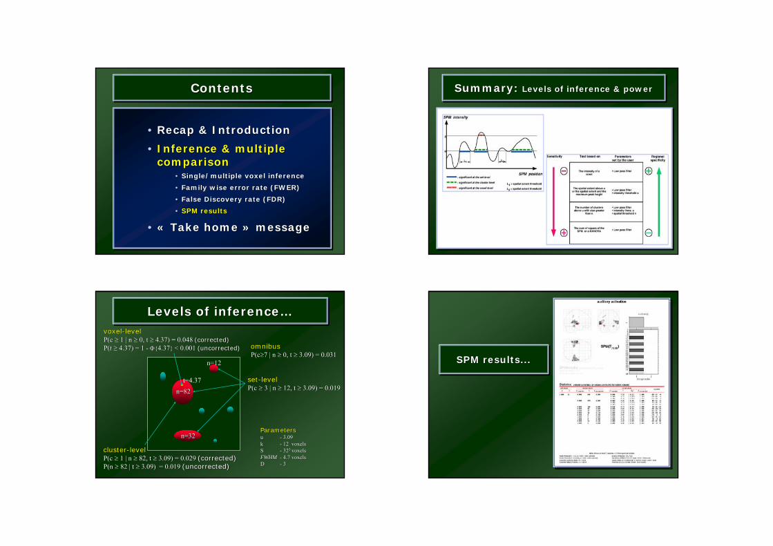
SPM position
u
SPM intensity
h
L1 L2
: significant at the set level
: significant at the cluster level
: significant at the voxel level
L1 > spatial extent threshold
L2 < spatial extent threshold
Regional specificity
Sensitivity
The intensity of a voxel
Test based on
The spatial extent above u or the spatial extent and the
maximum peak height
The number of clusters above u with size greater
than n
The sum of square of the SPM or a MANOVA
Parameters set by the user
• Low pass filter
• Low pass filter• intensity threshold u
• Low pass filter• intensity thres. u• spatial threshold n
• Low pass filter
Summary: Levels of inference & powerSummary: Summary: Levels of inference & powerLevels of inference & power
Levels of inference…Levels of inferenceLevels of inference……
ParametersParametersu u -- 3.093.09k k -- 12 voxels12 voxelsS S -- 32323 3 voxelsvoxelsFWHMFWHM -- 4.7 voxels4.7 voxelsD D -- 33
n=82n=82
n=32n=32
n=12n=12
omnibusomnibusP(cP(c≥≥7 | n 7 | n ≥≥ 0, t 0, t ≥≥ 3.09) = 0.0313.09) = 0.031
setset--levellevelP(c P(c ≥≥ 3 | n 3 | n ≥≥ 12, t 12, t ≥≥ 3.09) = 0.0193.09) = 0.019
clustercluster--levellevelP(c P(c ≥≥ 1 | n 1 | n ≥≥ 82, t 82, t ≥≥ 3.09) = 0.029 3.09) = 0.029 (corrected)(corrected)P(n P(n ≥≥ 82 | t 82 | t ≥≥ 3.09) = 0.019 3.09) = 0.019 (uncorrected)(uncorrected)
voxelvoxel--levellevelP(c P(c ≥≥ 1 | n 1 | n ≥≥ 0, t 0, t ≥≥ 4.37) = 0.048 4.37) = 0.048 (corrected)(corrected)P(P(tt ≥≥ 4.37) = 1 4.37) = 1 -- ΦΦ4.374.37 < 0.001 < 0.001 (uncorrected)(uncorrected)
t=4.37
SPM results...SPM results...SPM results...
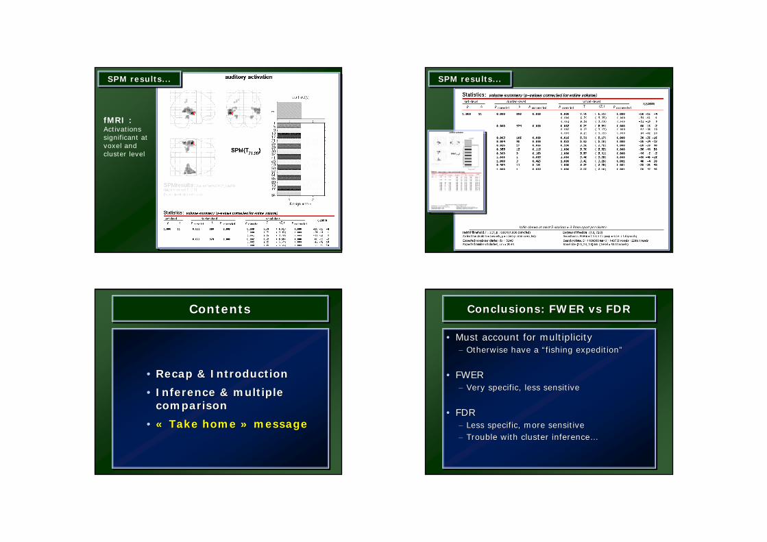
SPM results...SPM results...SPM results...
fMRI :Activations significant atvoxel andcluster level
SPM results...SPM results...SPM results...
ContentsContentsContents
• Recap & Introduction
• Inference & multiple comparison
• « Take home » message
•• RecapRecap & Introduction& Introduction
•• InferenceInference & multiple & multiple comparisoncomparison
•• «« TakeTake homehome »» messagemessage
Conclusions: FWER vs FDRConclusions: FWER Conclusions: FWER vsvs FDRFDR
• Must account for multiplicity– Otherwise have a “fishing expedition”
• FWER– Very specific, less sensitive
• FDR– Less specific, more sensitive– Trouble with cluster inference…
•• Must account for multiplicityMust account for multiplicity–– Otherwise have a Otherwise have a ““fishing expeditionfishing expedition””
•• FWERFWER–– Very specific, Very specific, lessless sensitivesensitive
•• FDRFDR–– Less specific, more sensitiveLess specific, more sensitive–– Trouble with cluster inferenceTrouble with cluster inference……
More Power to Ya!More Power to More Power to YaYa!!Statistical Power• the probability of rejecting the null hypothesis when it is
actually false• “if there’s an effect, how likely are you to find it”?
Effect size• bigger effects, more power
• e.g., MT localizer (moving rings - stationary runs) -- 1 run is usually enough
• looking for activation during imagined motion might require many more runs
Sample size• larger n, more power
• more subjects - longer runs - more runs
Signal:Noise Ratio• better SNR, more power
• stronger, cleaner magnet - more focal coil - fewer artifacts - more filtering