저 시-비 리- 경 지 2.0 한민

는 아래 조건 르는 경 에 한하여 게

l 저 물 복제, 포, 전송, 전시, 공연 송할 수 습니다.

다 과 같 조건 라야 합니다:

l 하는, 저 물 나 포 경 , 저 물에 적 된 허락조건 명확하게 나타내어야 합니다.

l 저 터 허가를 면 러한 조건들 적 되지 않습니다.

저 에 른 리는 내 에 하여 향 지 않습니다.

것 허락규약(Legal Code) 해하 쉽게 약한 것 니다.

Disclaimer

저 시. 하는 원저 를 시하여야 합니다.

비 리. 하는 저 물 리 목적 할 수 없습니다.

경 지. 하는 저 물 개 , 형 또는 가공할 수 없습니다.

경제학박사학위논문

Establishment Size, Industry, and Wage

Inequality: The Roles of Bonus and

Rent Sharing

사업체 규모, 산업과 임금 불평등:

보너스와 수익 배분의 역할을 중심으로

2017년 8월

서울대학교 대학원

경제학부 경제학 전공

송 상 윤

Abstract

Establishment Size, Industry, and Wage Inequality:

The Roles of Bonus and Rent Sharing

Sang-yoon Song

Department of Economics

The Graduate School

Seoul National University

Despite the growing evidence on the relation between bonuses (or

performance pay) and wage inequality, studies have focused on how

bonuses influence wage inequality among jobs. This study provides

new evidence on the large contribution of bonuses (i.e., performance

pay and non-production pay) to wage inequality among employers via

heterogeneous rent-sharing behaviors, focusing on industry affiliation

and employer size. Using comprehensive Korean worker-level data, I

first show that wage between-inequality at the industry-size level has

substantially contributed to a growing wage inequality trend since

1994 even after controlling for observed and unobserved worker char-

acteristics and factoring in sorting effects; this phenomenon is mainly

due to the differences in bonuses between industry-size groups, while

the effects of bonuses on within-inequality are limited. I then show

the sources of the rising wage between-inequality in terms of firm-side

i

factors using firm-level data merged with worker-level data at the

industry-size-year level. I find that changes in the estimated prices

of labor productivity (rent-sharing parameters) and the capital-to-

labor ratio are the main factors in the increasing dispersal of between-

inequality and that they became more positively correlated with wages

between 2009 and 2015 than they were before 2009. This positive cor-

relation is observed even more clearly when bonuses are included in

wages. These findings show that employers exhibit rent-sharing behav-

ior and compensate for capital dependency using bonuses, and bonus

differentials among employers are translated into increased between-

inequality of wages.

· · · · · · · · · · · · · · · · · · · · · · · · · · · · · · · · · · · · · · · · · ·

Keywords: Wage Inequality, Bonus, Establishment Size,

Industry, Labor Productivity, Capital-to-Labor Ratio, Rent-

Sharing Behavior

Student Number: 2014-30968

ii

Contents

1 Introduction 1

2 Data Description 7

2.1 WSS, KLIPS, and KED . . . . . . . . . . . . . . . . . 7

2.2 Sample Selection . . . . . . . . . . . . . . . . . . . . . 11

2.3 Two Types of Wages . . . . . . . . . . . . . . . . . . . 12

3 Trends in Between–Inequality of Wages 16

3.1 Simple Variance Decomposition . . . . . . . . . . . . . 16

3.2 Distributional Changes of Wages . . . . . . . . . . . . 20

4 Does Sorting Matter? 22

4.1 Trends in the Variances of Residuals . . . . . . . . . . 22

4.2 Full Variance Decomposition . . . . . . . . . . . . . . 25

4.3 Distributional Changes in Group Wage Premiums . . . 30

4.4 Effects of Unmeasured Worker Heterogeneity . . . . . 35

5 Firm–side Factors and Between–Inequality of Wages 39

5.1 Firm–side Factors . . . . . . . . . . . . . . . . . . . . . 42

5.2 Results I: Firm–side Factors and Wage Determination 44

5.3 Results II: Marginal Effects of Firm–side Factors on

Between–Inequality . . . . . . . . . . . . . . . . . . . . 48

5.3.1 Covariates Effects on Between–Inequality . . . 49

i

5.3.2 Coefficient Effects on Between–Inequality . . . 51

5.3.3 Marginal Effects of Covariates and Coefficients

on Changes in Between–Inequality . . . . . . . 53

6 Conclusion 58

7 Bibliography 62

8 Abstract in Korean 81

ii

List of Figures

1 Trends in Between–Group Variances: 1994–2015 . . . . 17

2 Changes in Average of Log Wages across Wage Per-

centiles (1994 vs. 2015) . . . . . . . . . . . . . . . . . . 21

3 Trends in the Variance of Residuals by Groups . . . . 24

4 Estimated Group Effect by Wage Percentiles (Industry–

size Level) . . . . . . . . . . . . . . . . . . . . . . . . . 31

5 Wage Premium Effects and Composition Effects by Wage

Percentiles . . . . . . . . . . . . . . . . . . . . . . . . . 33

6 Firm–side Factors by Wage Quantiles and Periods . . 49

7 The Estimate Results of Quantile Regression by Peri-

ods (Total Wages) . . . . . . . . . . . . . . . . . . . . 52

A1 The Comparison of Variances of (log) Hourly Total

Wages between Original Data and Sample Data . . . . 79

A2 The Estimated Results of Quantile Regression by Peri-

ods (Fixed Wages) . . . . . . . . . . . . . . . . . . . . 80

iii

List of Tables

1 The Comparison of Two Types of Wages by Industry

and Establishment Size . . . . . . . . . . . . . . . . . 15

2 Within– and Between–Variances by Groups and Their

Contributions . . . . . . . . . . . . . . . . . . . . . . . 19

3 The Results of A Full Variance Decomposition (Total

Wages) . . . . . . . . . . . . . . . . . . . . . . . . . . . 28

4 The Results of A Full Variance Decomposition (Fixed

Wages) . . . . . . . . . . . . . . . . . . . . . . . . . . . 29

5 The Changes in Wage Premiums and Worker Distribu-

tion by Establishment Size . . . . . . . . . . . . . . . . 34

6 Alternative Models of Control for Labor Quality (Industry–

size level, Total Wage) . . . . . . . . . . . . . . . . . . 37

7 The Effects of Unobserved Characteristics of Workers

(Industry–Size Level) . . . . . . . . . . . . . . . . . . . 38

8 The Effect of Firm–side Factors on Wage Determina-

tion: Industry–Size level . . . . . . . . . . . . . . . . . 46

9 The Counterfactual Variances by Covariates and Coef-

ficients Effects . . . . . . . . . . . . . . . . . . . . . . . 56

A1 The Number of Workers by Two–digit Industries – WSS 67

A2 The Number of Establishments by Two–digit Indus-

tries – KED . . . . . . . . . . . . . . . . . . . . . . . . 68

iv

A3 The Estimation Results of the Augmented Mincer-type

Wage Equation: Using Two–Digit Industry Dummies . 69

A4 The Estimation Results of the Augmented Mincer-type

Wage Equation: Using Industry–Size Dummies . . . . 70

A5 The Estimated Group Wage Premiums (Total Wage,

Year=1994) . . . . . . . . . . . . . . . . . . . . . . . . 71

A6 The Estimated Group Wage Premiums (Total Wage,

Year=2015) . . . . . . . . . . . . . . . . . . . . . . . . 73

A7 The Estimated Group Wage Premiums (Fixed Wage,

Year=1994) . . . . . . . . . . . . . . . . . . . . . . . . 75

A8 The Estimated Group Wage Premiums (Fixed Wage,

Year=2015) . . . . . . . . . . . . . . . . . . . . . . . . 77

v

1 Introduction

It is well-known that employers’ size and industry affiliation play im-

portant roles in explaining wage inequality among workers. Since the

seminal papers of Brown and Medoff (1989) and Krueger and Sum-

mers (1988), several studies have explored the sources of the positive

relation between employers’ sizes and wages workers are paid, and

wage differentials among industries.1 In a standard competitive la-

bor market model, one possible explanation for this phenomenon is

the difference in labor quality across employer sizes and industries.

Conflicting with this conventional explanation, however, empirical ev-

idence has shown that wage gaps among employers come mainly from

employers’ heterogeneous characteristics or behaviors such as labor

productivity, rent-sharing behavior, and technology dependence (e.g.,

Blanchflower et al., 1996; Arai, 2003; Faggio et al., 2010; Barth et al.,

2016). Using the intuitions of those works, this study attempts to de-

termine 1) how between-inequality at the industry and industry-size

levels has contributed to the rising wage inequality over the last two

decades in Korea and 2) their sources from the standpoint of firm-

side factors using firm-level data merged with worker-level data at

1Previous works on the effects of employer size on wages include Moore (1911),Oi and Idson (1999), Bayard and Troske (1999), Lluis (2009), and Pedace (2010).Lallemand and Rycx (2007) review the literature on this topic. Groshen (1991),Gibbons and Katz (1992), Vainiomaki and Laaksonen (1995), Gannon et al. (2007),and Lazear and Shaw (2009) study inter-industry wage premiums in several coun-tries.

1

the industry-size-year level. I also seek to shed light on the role of

bonus, including performance pay and non-production pay, in these

processes.

Amid the increasing accessibility of worker-level, firm-level, and

linked employer-employee longitudinal data in many countries, new

evidence has emerged on the significant contribution of employers to

wage inequality, which has helped to explain changes in wage inequal-

ity (e.g., Abowd, Kramarz, and Margolis, 1999; Card, Heining, and

Kline, 2013; Song et al., 2015). These studies identify both workers

and their workplaces, allowing wage inequality to be perfectly decom-

posed into within- and between-firm inequalities. Despite their impor-

tant contributions to finding the sources of wage inequality, however,

they have not closely examined the effects of industry affiliation and

employer size on wage inequality. I examine the contributions of em-

ployers’ industry and size on wage inequality by combining the Korean

Ministry of Employment and Labor’s Wage Structure Survey (WSS),

Korea’s largest worker-level database, which provides data on employ-

ers’ size and industry affiliation (using a two-digit code), with infor-

mation on worker characteristics and representative firm-level balance

sheet data taken from the Korea Enterprise Database (KED). Com-

bining these two data sources produces a longitudinal dataset that

contains comprehensive information on employees and employers at

the industry-size-year level.

2

This study is novel in its focus on the role of bonuses in explain-

ing wage inequality. The wage-setting system of the typical firm in

Korea is a combination of fixed wages and bonuses; and the negotia-

tions for wages are conducted at firm-level (decentralized industries).2

Fixed wages are the contracted wages that must be paid regardless of

the workers’ and firms’ performance. They are anchored by job po-

sition and increase along with promotion. By contrast, bonuses vary

depending on the firm’s situation and the worker’s abilities. Some

firms introduce bonuses mainly to obtain strategic flexibility of wage-

setting and to hedge their performance risk. In this case, the entire

performance of the firm and favorability to sharing rents with work-

ers are closely linked to the amount of bonuses workers are paid. This

leads to the increase of wage inequality between firms. Other firms

use bonuses mainly to compensate different workers disproportion-

ately. This can increase wage inequality within firms. In sum, bonus

amounts are driven by three factors: the performance of the worker,

the performance of his or her employer, and the attitude of the em-

ployer to sharing rents with workers. The performance of a worker

may be evaluated as high; however, if the performance of the firm

is poor, the worker will not be sufficiently compensated for his abil-

2Rusinek and Rycx (2013) investigate the impact of different collective bar-gaining arrangements on the relationship between firms’ profitability and wagesvia rent-sharing. They show that in industries where agreements are usually rene-gotiated at firm-level (decentralized industries) wages and firm-level profits aremore positively correlated than industries where firm-level wage renegotiation isless common (centralized industries).

3

ity. Moreover, if a highly profitable firm is not favorable to sharing

rents with workers, its bonuses may be relatively low. Either of these

situations may cause bonuses to affect wage inequality.

This study has two objectives. The first is to investigate how

changes in between-inequality at the industry and industry-size levels

influence changes in overall wage inequality between 1994 and 2015

in Korea. I show that the changes in inequality between industry-size

groups have significantly contributed to the changes in overall wage

inequality even when workers’ observed and unobserved character-

istics are controlled for and that this phenomenon has been ampli-

fied by the systematical differences in bonuses between industry-size

groups. The second objective is to explore the sources of the con-

tribution of between-inequality using firm factors such as labor pro-

ductivity and the capital-to-labor ratio. I decompose their contribu-

tions into “quantity effects” and “price effects” following Machado and

Mata (2005), and show that employers’ heterogeneous rent-sharing

behaviors along the wage distribution is a main element of the rising

between-inequality.

This paper complements recent empirical works on wage deter-

mination and inequality. Blanchflower et al. (1996) provided a the-

oretical background on the relation between wages and employers’

rent-sharing behavior. Using the wage bargaining model, they derived

a simple wage equation and empirically demonstrated the positive

4

association between wages and employers’ rent-sharing behavior by

blending microeconomic data on wages with industrial data. Using

Swedish data on workers matched with firms’ balance sheets, Arai

(2003) showed that wages are positively correlated with the capital-

to-labor ratio as well as employers’ profits. Barth et al. (2016) showed

that the change in wage variance among establishments contributes

65% of the increased variance in earnings from 1992 to 2007 in the

U.S. They also showed that the wage gap between two-digit indus-

tries is an important factor in making wage inequality among estab-

lishments more dispersed. Lemieux et al. (2009) demonstrated the

importance of performance pay in explaining wage inequality using

data from PSID. They focused on the contribution of performance

pay to within-inequality by comparing between performance-pay jobs

and non-performance-pay jobs. They concluded that compensation for

performance-pay jobs was more closely tied to worker characteristics

and that changes in returns to skill due to technological change in-

duced more firms to offer performance pay. I expand their analyses

to examine the contributions of bonuses to wage inequality among

employers in Korea.3 Concerning methodology, Machado and Mata

(2005) provide a method that allows me to observe the marginal ef-

fects of firm-side factors on wage inequality using quantile regression

and integral transformation theorem.

The empirical results of this paper confirm that the rising trends

3See section 3.2 for the difference between bonus and performance pay.

5

in Korean wage inequality between 1994 and 2015 are associated

with trends in between-inequality at the industry-size level rather

than at the industry level. The industry-size level change in between-

inequality contributes 44.03% of the change in wage inequality even

after workers’ observed characteristics and sorting effects are con-

trolled for, while the industry-level contribution amounts to 11.33%.

This means that the wage gap between employers of different sizes

is the main factor in between-inequality. The contribution of indus-

try size to between-inequality decreases to 29.35% when bonuses are

not considered. This large drop shows that bonus differentials be-

tween industry-size groups play important roles in explaining between-

inequality trends. Interestingly, the results of the longitudinal data

show that the contributions of workers’ unobserved characteristics to

wage inequality trends are minor in spite of their large contribution

to wage inequality levels, while the large contribution of between-

inequality to wage inequality trends remains.

Investigating the sources of the changes in between-inequality from

2000 to 2015 shows that changes of rent-sharing parameter and the

prices of capital–labor ratio are the main factors in the rising between-

inequality. They become more positively correlated with wages be-

tween 2009 and 2015 than they are before 2009. The positive corre-

lations are observed even more clearly when bonuses are included in

wages. The changes in rent-sharing parameters between the two pe-

6

riods make between-inequality, measured as the variance in log real

hourly wages, change from 0.131 to 0.1879, while between-inequality

changes from 0.0901 to 0.0998 when bonuses are not considered. The

change in the capital-to-labor ratio price shows similar effects on the

change in between-inequality. These results imply that paying bonuses

is one way firms share their rents with workers and compensate for

heavy capital dependency.

The remainder of this paper is organized as follows. Section 2

describes the data and the sample selection process. Section 3 dis-

cusses the trends in wage inequality, focusing on a comparison be-

tween within- and between-inequality. Section 4 presents the results

of a full variance decomposition, using the augmented Mincer-type

earning equation, to control for worker characteristics and observe the

contribution of between-inequality to wage inequality. Section 5 inves-

tigates the effects of firm-side factors on between-inequality trends.

Finally, section 6 concludes the paper.

2 Data Description

2.1 WSS, KLIPS, and KED

WSS and KLIPS: Worker–level Data

The Wage Structure Survey (WSS) dataset is the largest worker-level

dataset in Korea, with information on approximately 500,000 regu-

7

lar workers per year provided by the Korea Ministry of Employment

and Labor. The survey has been conducted each June since 1980. The

WSS data include monthly wage and hours worked in a month, as well

as information on education, occupation, experience, union participa-

tion, gender, industry (two-digit code), and employer size (measured

by the number of employees and comprising five categories: 10–29,

30–99, 100–299, 300–499, and 500+).4,5 Since 2006, this dataset has

also been providing establishment identifiers that can be used to ob-

serve the effects of firm heterogeneity on wage inequality.6

There are three advantages to using this dataset to study wage

inequality. First, total monthly wages can be decomposed into regular

wages, overtime wages, and bonuses. The provision of bonuses al-

lows us to identify their effects on wage inequality. Second, the WSS

is relatively free of measurement error because it has been gathered

by establishment-level surveys.7 Third, the survey is designed to con-

trol for sampling errors regarding industry and establishment size and

provides a weight for each worker.8 These weights allow the data to

4One employer size category, 5–9, has been added since the 1999 survey. Tomaintain data consistency, employees working in firms with fewer than 10 employ-ees are excluded.

5The WSS data do not provide an industry classification more detailed thanthe two-digit codes. Barth et al. (2016) demonstrated that expanding industrialcategories from one-digit to two-digits contributes significantly to wage inequality,while the effects of more detailed categories are modest.

6Unfortunately, since these establishment identifiers are randomly assigned bythe Korea Ministry of Employment and Labor, I cannot combine this dataset withestablishment-level micro data due to the absence of common identifiers.

7As the survey is implemented using firms’ payrolls, measurement errors aremuch smaller than those of individual-level surveys.

8The Korea Ministry of Employment and Labor determines a worker’s weightaccording to three factors: the design weight of the employee’s workplace, the

8

represent the average worker rather than the average industry or size.

All of the estimates reported in this paper are weighted using the

sample weights.

The critical limitation of the WSS dataset for studying wage in-

equality is that self-employed workers, non-regular workers, and work-

ers working in establishments with fewer than five employees cannot

be considered due to the survey design. Since this limitation may lead

to a biased evaluation of the overall inequality of wages in Korea, the

results have to be interpreted for regular workers in establishments

with more than five employees. Another limitation is that, as the

WSS comprises cross-sectional data, unobserved heterogeneity among

workers cannot be controlled for.9

To observe the effects of unobserved worker heterogeneity on wage

inequality and check the robustness of the results derived from the

WSS data, I use Korean Labor and Income Panel Study (KLIPS)

data, which have longitudinal features and provide information on

workers similar to that provided by the WSS for the 1998–2015 period.

Unfortunately, the KLIPS data provide information on only 5,000

regular employees each year and is thus less representative. However,

as wage inequality (measured by the variance in log real hourly wages)

probability of sampling the worker, and a post-stratification adjustment coefficient.The Ministry also outlines its method of using the weight.

9Several recent studies on wage inequality using large longitudinal workerdatasets have reported that unobserved heterogeneity among workers contributessignificantly to changes in wage inequality in the U.S. and Germany (e.g., Card,Heining, and Kline, 2013; Song et al., 2015).

9

in the two datasets shows similar rising trends between 1998 and 2008,

there appears to be no serious problem with using the KLIPS to check

the robustness of the results from the WSS.

KED: Firm–level Balance Sheet Data

The Korea Enterprise Database (KED) offers data on financial state-

ments and the number of regular workers at Korean firms in order

to assign credit ratings. It covers 2000 to 2015 and 50% of Korean

firms.10 This database is useful for studying wage inequality because

it includes many small firms with fewer than 50 regular employees, un-

like other available firm-level balance sheet data. In 2015, small firms

with fewer than 50 employees accounted for 89.32% of all firms, and

their share of sales was 22.7%. The high share of small firms and their

low share of sales clearly reflect the skewed distributional structure

among Korean firms.

Merged Data

To observe the effects of worker characteristics and firm-side factors

on wage inequality, worker- and firm-level data must be merged into

one dataset. Because the worker-level datasets (WSS, KLIPS) do

not provide public firm identifiers, I cannot construct a linked em-

ployer–employee dataset like the U.S. Longitudinal Employer House-

10According to Korea’s National Tax Service, firms with more than 10 regularemployees totaled about 145,000 in 2014, and the KED covers about 70,700 firms.

10

hold Dynamics (LEHD). However, data on industry (two-digit), estab-

lishment size (five categories), and year can be used to link between

worker- and firm-level data. Thus, I aggregate the WSS and KED us-

ing industry-size identifiers per year and combine them to construct

longitudinal data at the industry-size level.11 Although inequality be-

tween firms cannot be observed using the combined dataset, inequality

between industry-size groups and its sources can be captured using

worker- and firm-side variables aggregated in industry-size cells.

2.2 Sample Selection

For the main analysis, samples are restricted to regular workers be-

tween the ages of 20 and 60. I exclude those who work fewer than 10

days per month and who earn less than the minimum hourly wage.12

I also exclude the agriculture industry and several industries in ser-

vice sector, such as education, health, and social work (e.g., hospital),

as well as arts-, sports-, and recreation-related services (e.g., creativ-

ity and arts-related services), membership organizations, repair and

other personal services (e.g., labor organizations and religious orga-

11One possible criticism of this process is that the WSS provide establishment-level data, while the KED provides firm-level data. As Korea is a small country, itsnumbers of establishments and firms do not differ significantly. According to KoreaStatistics, the number of establishments and firms with more than five regularemployees total 68,989 and 65,059 in the manufacturing sector, respectively. Firmswith more than two establishments constitute conglomerates such as Samsung andHyundai. As establishments in such conglomerates have more than 500 employees,the biases induced by combining establishment-level and firm-level data are notlarge enough to contaminate the main results of this study.

12The share of workers who earn less than the minimum hourly wage accountsfor less than 1% of the observations. Considering such wages could lead to mea-surement errors.

11

nizations), and extraterritorial organizations; the association between

wages and firm characteristics are not likely to be meaningful in those

industries. The Korean government has revised its industry classifi-

cation twice, in 2000 and 2007 (i.e., the 8th and 9th Korea Standard

Industry Classification [KSIC], respectively) since 1994. Because the

recent revision provides more detailed classifications, I aggregate some

industries for time-series consistency over the analysis periods.13 The

manipulation of industry classification applies equally to all datasets

(i.e., WSS, KLIPS, KED). The number of workers in the WSS data

and firms in the KED (two-digit industries) are presented in Table

A1 and A2 in the appendix. Figure A1 in the appendix presents the

wage variance trends in the original WSS data and the sample data

restricted by the criteria mentioned above. The gap between the two

lines is minor, indicating that the effect of the sample restrictions on

wage inequality trends is small.

2.3 Two Types of Wages

Two types of real (adjusted by CPI, 2015=100) hourly wages, fixed

and total wages, are used in this study. Their definitions are as follows:

Hourly Fixed Wage =regular wage + overtime wage

working hours(1)

13For instance, the food and beverage industries belonged to the same industryunder the two-digit classification in the 7th and 8th KSIC but were separated in the9th KSIC. Thus, I integrated them after 2007 to maintain classification consistency.

12

Hourly Total Wage = hourly fixed wage +bonus/12

working hours(2)

As mentioned in section 2.1, while regular wage, overtime wage, and

working hours provided in the WSS data are monthly (based on the

June of each year), bonuses are yearly data. They are thus divided by

12 to convert yearly data into monthly data. The difference between

the two types of wages concerns whether bonuses are included; the

difference in their variance can therefore be interpreted as the effects

of bonuses on wage inequality.

I must address the difference between performance pay and bonuses.

Unlike previous works such as Lemieux et al. (2009) and Bryan and

Bryson (2016), this study uses the term “bonus” instead of “per-

formance pay” because the bonuses considered in this paper include

non-production pay, defined as cash payments that are not explicitly

related to formula for productivity, such as holiday bonuses.14,15 One

can argue that non-production pay must be included in fixed wages

because it is determined by wage contracts. Non-production pay is

closer to bonuses, however, for two reasons: 1) the differences in non-

14This definition of “non-proudction pay” is taken from Gittleman and Pierce(2015).

15Considering several types of wages, Gittleman and Pierce (2015) consider ajob to be a performance-pay job if either of two conditions holds: the job has non-production bonuses such as holiday bonuses and cash profit-sharing bonuses; orit has wages tied to commissions, piece-rate wages, production bonuses, or otherincentives. They use “incentive-pay jobs” to denote jobs that meet only the secondcondition. By contrast, Lemieux et al. (2009) and Bryan and Bryson (2016) defineperformance-pay jobs as jobs for which wages are, at least partly, determined byvariable pay components such as bonus, commission, and piece-rate.

13

production pay among firms are great, as large firms typically provide

non-production pay as a fringe benefit, while most small firms provide

none at all; 2) non-production pay can be more easily adjusted than

fixed wages can. Gittleman and Pierce (2015) also pointed out that

non-production payments stem from annual bonus plans but may also

reflect a variety of incentive plans.

Table 1 shows the average log real hourly wages by industry (one-

digit) and establishment size using data from the WSS. The weighted

standard deviations (labeled “Weighted S.D.”) are calculated using

the weights provided in the WSS data. Two things are to be noted.

First, the weighted S.D. of industry average wages and the wage dif-

ferences between size 1 (10–29) and size 5 (500+), labeled “Size 5–Size

1”), are larger for total wages than for fixed wages in all years. This

indicates that bonuses are a factor in making the wage distribution

more dispersed. Second, while the differences in the weighted S.D. of

industry average wages between the total wage and fixed wage are rel-

atively stable over time, the differences in wages between size 1 and

size 5 become much larger as time goes on.

14

Table 1: The Comparison of Two Types of Wages by Industry and Establishment Size

Industry and Size

Average of (log real hourly) Wages

1994 2008 2015

Total Fixed Total Fixed Total Fixed

Industry (one-digit)

Mining and Quarrying 0.0423 -0.1373 0.5906 0.4346 0.5831 0.4452

Manufacturing -0.2561 -0.4705 0.3845 0.1781 0.5230 0.3469

Electricity, Gas, Steam and Water Supply 0.1848 -0.1005 1.0061 0.7098 1.0684 0.8429

Construction 0.0559 -0.1170 0.4300 0.3312 0.6670 0.5849

Wholesale and Retail Trade -0.1761 -0.3701 0.4473 0.2915 0.4102 0.2916

Accommodation and Food Service Activities -0.2971 -0.4703 0.0401 -0.0447 -0.0128 -0.0462

Transportation -0.1796 -0.3489 0.4345 0.2608 0.4504 0.3193

Financial and Insurance Activities 0.2542 -0.0964 0.9156 0.6283 0.9403 0.6971

Real Estate Activities and Renting and Leasing -0.3942 -0.5837 0.2184 0.1203 0.2781 0.2112

Weighted S.D. 0.1678 0.1414 0.1777 0.1482 0.1728 0.1415

Establishment Size (Five Categories)

Size 1: 10–29 -0.2441 -0.3955 0.2633 0.1521 0.3456 0.2523

Size 2: 30–99 -0.2700 -0.4449 0.3104 0.1743 0.3798 0.2767

Size 3: 100–299 -0.1818 -0.4026 0.4204 0.2284 0.4455 0.2931

Size 4: 300–499 -0.0874 -0.3476 0.6388 0.4022 0.6580 0.4474

Size 5: 500+ 0.0324 -0.2829 0.8799 0.5117 1.0991 0.7563

Log Differences: Size 5-Size 1 0.2765 0.1125 0.6166 0.3596 0.7535 0.5040

Notes. This table shows the average log real hourly wages by industry (one-digit) and establishment size using data from the WSS. The difference betweentotal wages and fixed wages concerns whether bonuses are included. The weighted standard deviations (labeled “Weighted S.D.”) are calculated using theworkers’ weights provided in the WSS data.

15

3 Trends in Between–Inequality of Wages

In this section, I first conduct a simple variance decomposition to

observe the trends in wage inequality within and between groups us-

ing the WSS data without considering worker characteristics. I then

observe the distributional features in the changes in wage inequality

by wage percentiles to determine which wage percentiles are more af-

fected by between-inequality. Industry (two-digit), industry-size (two-

digit and five categories), and establishments are treated as groups to

observe their contributions to wage inequality.

3.1 Simple Variance Decomposition

The variance of log real hourly wages can be decomposed into two

components, within- and between-variance. Let wi,g be the log real

hourly wage of worker i in group g, and wg be the average log real

wages of workers employed by group g. The two variances can be

expressed by the following equations where V ar(wg) and V ar(wi,g −

wg) present the between- and within-variance, respectively:

wi,g ≡ wg + (wi,g − wg) (3)

V ar(wi,g) = V ar(wg) + V ar(wi,g − wg) (4)

I calculate each variance of equation (4) using the workers’ weights,

θi,g, provided by the WSS data, where the sum of the weights is equal

16

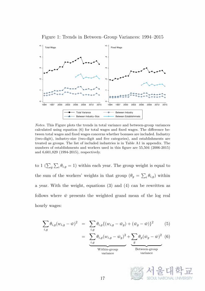
Figure 1: Trends in Between–Group Variances: 1994–20150

.1.2

.3.4

.5

1994 1997 2000 2003 2006 2009 2012 2015

Total Wage

0.1

.2.3

.4.5

1994 1997 2000 2003 2006 2009 2012 2015

Fixed Wage

Total Variance Between Industry

Between Industry−Size Between Establishmnets

Notes. This Figure plots the trends in total variance and between-group variancescalculated using equation (6) for total wages and fixed wages. The difference be-tween total wages and fixed wages concerns whether bonuses are included. Industry(two-digit), industry-size (two-digit and five categories), and establishments aretreated as groups. The list of included industries is in Table A1 in appendix. Thenumbers of establishments and workers used in this figure are 55,504 (2006-2015)and 6,601,829 (1994-2015), respectively.

to 1 (∑

g

∑i θi,g = 1) within each year. The group weight is equal to

the sum of the workers’ weights in that group (θg =∑

i θi,g) within

a year. With the weight, equations (3) and (4) can be rewritten as

follows where w presents the weighted grand mean of the log real

hourly wages:

∑i,g

θi,g(wi,g − w)2 =∑i,g

θi,g{(wi,g − wg) + (wg − w)}2 (5)

=∑i,g

θi,g(wi,g − wg)2

︸ ︷︷ ︸Within-group

variance

+∑g

θg(wg − w)2

︸ ︷︷ ︸Between-group

variance

(6)

17

Figure 1 plots the trends in total variance and between-group vari-

ances calculated using equation (6) for total wages and fixed wages.

There are two notable features in Figure 1. First, although the levels

and trends of between-industry variance (shown by the line marked

with diamonds) are relatively stable over time, the variance between

industry-size groups (shown by the line marked with triangles) shows

an increasing trend between 1994 and 2008. This suggests that the ris-

ing wage inequality is more attributable to the increase in the variation

in wages across establishment sizes than to that across industries. This

pattern is clearer in the left plot for total wages, indicating that differ-

ences in bonuses between establishment sizes play an important role

in the widening between-inequality at the industry-size level. Second,

the variance between industry-size groups contributes significantly to

the between-establishment variance (shown by line marked with +).

In the left plot for total wages, the contributions of the variances be-

tween industry-size groups to the variances between establishments

account for 51.6% (=0.1137/0.2204) and 54.6% (=0.1117/0.2046) of

the total in 2006 and 2015, respectively, suggesting that industry and

establishment size play an important role in explaining the effects of

establishment heterogeneity on wage inequality.

Table 2 summarizes the results of the simple variance decomposi-

tion for the two types of wages. The variance between industries con-

tributes 4.4% of the increased variance of total wages between 1994

18

Table 2: Within– and Between–Variances by Groups and Their Con-tributions

Group Variance 1994 2001 2008 20152015-1994

Change Share

Total Wage

Total 0.2546 0.3105 0.3965 0.3355 0.081

IndustryWithin 0.2017 0.2477 0.3231 0.2791 0.077 0.956

Between 0.0529 0.0628 0.0733 0.0564 0.004 0.044

Industry+SizeWithin 0.1825 0.2108 0.2643 0.2238 0.041 0.511

Between 0.0721 0.0998 0.1322 0.1117 0.040 0.489

EstablishmentWithin - - 0.1494 0.1309

Between - - 0.2471 0.2046

Fixed Wage

Total 0.1940 0.2288 0.3007 0.2525 0.059

IndustryWithin 0.1598 0.1897 0.2516 0.2178 0.058 0.992

Between 0.0342 0.0391 0.0491 0.0347 0.000 0.008

Industry+SizeWithin 0.1512 0.1722 0.2257 0.1929 0.042 0.713

Between 0.0428 0.0566 0.0750 0.0596 0.017 0.287

EstablishmentWithin - - 0.1308 0.1169

Between - - 0.1699 0.1356

Notes. This table shows contributions of changes in within- and between-variances tochanges in wage variances. The difference between total wages and fixed wages concernswhether bonuses are included. Industry (two-digit), industry-size (two-digit and five cat-egories), and establishments are treated as groups. The list of included industries is inTable A1 in appendix. The numbers of establishments and workers used in this figure are55,504 (2006-2015) and 6,601,829 (1994-2015), respectively.

and 2015, while the variance between industry-size groups contributes

48.9%. Although this pattern is commonly observed for fixed wages,

the magnitudes of the contributions of between-inequality (0.8% at the

industry level and 28.7% at the industry-size level) are much smaller

due to the absence of the effects of bonuses.

19

3.2 Distributional Changes of Wages

The variance in log real hourly wages, a simple statistic for inequal-

ity, cannot capture the distributional features of wages. To determine

which percentiles cause the increased wage inequality between 1994

and 2015, I calculate the wage differences between the two years by

wage percentiles. Specifically, I first group the samples into 100 wage

percentile bins per year. Then, I calculate the average of log wages

and of the mean wages of the industry, and then do the same for the

industry-size groups for each percentile. Finally, I calculate the differ-

ences of each average value between 1994 and 2015 by wage percentile.

Figure 2 shows the distributional changes in wages between 1994

and 2015. The left plot is for total wages and the right one is for

fixed wages. Three phenomena revealed through the comparison be-

tween the two plots are worth mentioning. First, the upward slopes

of wages (shown by the black line, labeled “Avg of Wages”) observed

in both plots (except for the range below about the 20% percentile)

indicate that workers at the upper distribution earn more than those

at the bottom. Moreover, the upward slope is much steeper for to-

tal wages than for fixed wages, indicating that bonuses make the

wage distribution more dispersed. Second, the comovement between

the average of wages (shown by the black lines) and the average of

wages at the industry-size level (shown by the dark gray lines, labeled

“Avg of Wages at industry-size”) is much stronger for total wages

20

Figure 2: Changes in Average of Log Wages across Wage Per-centiles (1994 vs. 2015)

.4.5

.6.7

.8.9

1

Log C

hanges (

2015−

1994)

0 10 20 30 40 50 60 70 80 90 100

Percentiles of Log Wages

Total Wage

.4.5

.6.7

.8.9

1

Log C

hanges (

2015−

1994)

0 10 20 30 40 50 60 70 80 90 100

Percentiles of Log Wages

Fixed Wage

Avg of Wages Avg of Wages at Industry−Size

Avg of Wages at Industry

Notes. This figure shows the distributional changes in wages between 1994 and2015. The left plot is for total wages and the right one is for fixed wages. X-axis is100 wage percentile bins per year. Y-axis is log changes of average of wages and ofthe mean wages of the groups at the corresponding bins between 1994 and 2015.The list of included industries is in Table A1 in appendix.

than for fixed wages. The correlations between the two lines are 0.892

and 0.684, respectively. This means that the bonus differential be-

tween industry-size groups is a crucial factor in the widening wage

gaps among workers. Third, the gap between the average of wages at

the industry-size level and the average of wages at the industry level

(shown by the dark and thin gray lines respectively) is broader when

bonuses are considered. This shows that the changes in bonuses by

wage percentile between the two years are attributable to the bonus

differentials between establishment sizes rather than those among in-

dustries, as shown in Figure 1 and Table 2.

21

4 Does Sorting Matter?

Does the rising wage inequality between industry-size groups come

mainly from sorting effects or pure group effects? This section answers

this question. The sorting effects would cause the differentials in labor

quality to lead to wage inequality between groups. If the sorting effects

explain most of the trend in between-inequality, the contribution of

industry-size effects to wage inequality would come not from their own

characteristics but from the differences in labor quality.

4.1 Trends in the Variances of Residuals

Using the WSS data, I estimate the following augmented Mincer–type

wage equation for the 1994–2015 period based on Barth et al. (2016)’s

model:

wi,g = xi,gb+ ϕg(i) + ui,g, with E(ui,g|xi,g, ϕg) = 0 (7)

In this equation, wi,g is a vector of log real hourly wages for worker i in

group g; xi,g is a set of independent variables for worker characteristics

(years of schooling, experience and its square [Mincer], union partic-

ipation, occupation dummies [nine categories], and interaction terms

for each variable with gender); and ϕg(i) is a vector of dummy vari-

ables for group g shared by workers employed in group g. The residual

ui,g captures unobserved factors such as worker-group match effects,

22

unobservable worker characteristics, and purely transitory wage fluc-

tuations. To allow the prices of worker characteristics to vary over

time, all models are fitted separately by year.

One way to observe how the effect of each group contributes to

wage inequality is to compare the trends in residuals estimated by dif-

ferent groups. I conduct four regressions using equation (7) for several

groups: no group (worker characteristics only), industry, industry-size,

and establishment. The four regressions have the same independent

variables for worker characteristics, but the group dummies are dif-

ferent. Owing to data constraints, the regressions using establishment

dummies are conducted from 2006 to 2015. The regression results at

industry and industry-size level are in Table A3 and A4 in appendix.

Figure 3 plots the weighted variances of residuals estimated by

the four regressions. The top line (marked with circles) of the figure

is the trend of the weighted variance of log wages shown in the ear-

lier section. The second line (marked with X) is the variance of the

residuals from equation (7) with no group dummies. Although worker

characteristics explain a large portion of the total variance, the trend

in the residual variance is similar to the trend in the total variance

of wages. This indicates that the changes in wage inequality cannot

be fully accounted for by worker characteristics only. The third line

(marked with diamonds) and fourth line (marked with triangles) are

the variances of the residuals from the models with two-digit industry

23

Figure 3: Trends in the Variance of Residuals by Groups0

.1.2

.3.4

.5

1994 1997 2000 2003 2006 2009 2012 2015

Total Wage

0.1

.2.3

.4.5

1994 1997 2000 2003 2006 2009 2012 2015

Fixed Wage

Total Variance No Group Industry

Industry−Size Establishment

Notes. This figure shows the trends of the weighted variances of residuals estimated bythe four regressions using equation (7) for several groups. The difference between totalwages and fixed wages concerns whether bonuses are included. “No Group,’’ “Industry,’’“Industry-Size,’’ and “Establishment’’ denote the variances of the estimated residualsusing the worker characteristics (W.C.) only, W.C. + industry dummies, W.C. + industry–size dummies, and W.C. + Establishment dummies as regressors, respectively.

dummies and industry-size dummies, respectively. One notable feature

of these two lines is the difference between each line and the second

line. The difference between the second line and third line is sta-

ble over time, suggesting that the contributions of between-inequality

at the industry level to changes in wage inequality are limited. By

contrast, the difference between the second line and the fourth line

increases over time. This reveals that size effects dominate the impact

of industry-size groups on wage inequality trends. The last line shows

a substantial contribution of establishment heterogeneity in explain-

ing both the levels and changes in wage inequality. The contribution

of establishment heterogeneity to wage inequality levels can be mea-

24

sured by the difference between the second line and the last line. The

flat shape of this line means that the trends that are not explained

by industry-size group effects are attributable to establishment het-

erogeneity.

Finally, the most important feature observed in Figure 3 is the

difference between the left panel, for total wages, and the right panel,

for fixed wages. Although the phenomena explained above are ob-

served in both panels, the industry and industry-size group effects

observed in the left panel for total wages seem to make a large con-

tribution to wage inequality. As mentioned, this phenomenon denotes

that bonuses have played an important role in the contribution of

between-inequality to overall wage inequality. To add such interpre-

tation, the difference between two panels implies that the substantial

contribution of the bonuses to between-inequality has not came from

worker characteristics. The fact that the amount of bonuses that is

paid by employers are less related to the observed labor quality pro-

vides a possibility that it would be more related to firm-side factors

unless sorting effects dominate the effects of between-inequality on

trends in wage inequality.

4.2 Full Variance Decomposition

In the previous section, by observing the estimated residuals trend by

group, I confirm the large contribution of between-inequality at the

industry-size level to the rising trends in wage inequality. As men-

25

tioned, this large contribution comes from two components: pure ef-

fects and sorting effects. I decompose between-group variance into

these two effects using equations (8) and (9) formed by taking the

variance of equation (7), where ρ (=Cov(xb, xbg)/V ar(xb)) is the

worker–worker segregation index across groups suggested by Kremer

and Maskin (1996), and ρϕ(= Cov(xb, ϕ)/V ar(xb)) is a worker-group

segregation index: 16

V ar(w) = V ar(xb) + V ar(ϕ) + 2Cov(xb, ϕ) + V ar(u) (8)

= V ar(xb)(ρ+ 2ρϕ)︸ ︷︷ ︸sorting effect

+ V ar(ϕ)︸ ︷︷ ︸group effects︸ ︷︷ ︸

Between-groupvariance

+V ar(xb)(1 − ρ)︸ ︷︷ ︸Within-group

variance

+V ar(u)(9)

Here, ρ shows the sorting effect by worker characteristics. If a firm em-

ploys workers randomly by observed characteristics, then ρ = 0. When

a firm hires observably similar workers, ρ will be close to 1. Similarly,

ρϕ captures the sorting effect between observed worker characteristics

and group wage premiums. If the observably more qualified workers

are hired in groups with higher wages, then ρϕ will be close to 1.17

The values of interest in equation (9) are the extent of the ratio of

16Barth et al. (2016) treated Var(u) as within-group variance. If establishmenteffects are completely controlled by group dummies, Var(u) can be treated aswithin-group variance, as in Barth et al. (2016). In this paper, however, since onlyindustry or industry-size effects are controlled, establishment effects that are notcaptured by industry or industry-size effects remain error terms. Thus, Var(u) isnot included in within-group variance.

17Since the worker-group segregation index, ρϕ, comes from the covariance termin equation (8), the difference between equations (8) and (9) concerns whether toconsider the worker-worker segregation index. If the worker-worker segregationindex has a negligible quantity, we can measure the sorting effects using the co-variance term in equation (8). The estimated worker-worker segregation index is0.133, 0.186, and 0.175 in 1994, 2008, and 2015, respectively. I consider that thesefigures are not negligible.

26

group effects to overall variance, V ar(ϕ)/V ar(w), and its trend over

time.

Table 3 and 4 show the results of a full variance decomposition

for total wages and fixed wages using equation (9). When industries

are treated as groups, the share of the change in variance of total

wages between 1994 and 2015 is largely explained by the change in

variance of the residuals (66.53%). Moreover, the change in variance

between industries explains just 11.33% of the change in the variance

of total wages. These results indicate that observed worker character-

istics and employer industry affiliation cannot fully account for the

trend in the variance of total wages. By contrast, the contribution

of the residual decreases to 37.94% when industry-size is treated as

groups. Furthermore, what dominates the increased variance in to-

tal wages is the increased inequality between industry-size groups

(62.2%), which is attributable mainly to group effects, not sorting

effects. The group effects account for the bulk of the between-group

variance (0.4403/0.662=66.5%), and, while the variance in total wages

decreases from 0.3956 to 0.3596 between 2008 and 2015, the variance

between industry-size groups increases from 0.0803 to 0.0828. The de-

creasing variance in total wages is due to within and residual variances.

This means that, though wage inequality shows a decreasing trend be-

tween 2008 and 2015, the group effects at the industry-size level are

increasing since 1994, and the decreasing trend of between-inequality

27

Table 3: The Results of A Full Variance Decomposition (Total Wages)

Group Variance 1994 2002 2008 20152008-1994 2015-1994

Change Share Change Share

Total 0.2546 0.3535 0.3965 0.3596 0.1419 1.0000 0.1050 1.0000

Industry

Between 0.0529 0.0834 0.0733 0.0734 0.0205 0.1442 0.0205 0.1950

Group effect 0.0225 0.0426 0.0375 0.0344 0.0149 0.1051 0.0119 0.1133

Sorting effect 0.0303 0.0408 0.0359 0.0389 0.0055 0.0391 0.0086 0.0818

Within 0.0990 0.1237 0.1329 0.1136 0.0339 0.2391 0.0147 0.1397

Residual 0.1028 0.1465 0.1903 0.1726 0.0875 0.6167 0.0699 0.6653

Industry+Size

Between 0.0722 0.1264 0.1370 0.1375 0.0649 0.4571 0.0653 0.6220

Group effect 0.0365 0.0641 0.0803 0.0828 0.0438 0.3085 0.0462 0.4403

Sorting effect 0.0356 0.0623 0.0567 0.0547 0.0211 0.1485 0.0191 0.1817

Within 0.0890 0.0957 0.1044 0.0888 0.0154 0.1089 -0.0001 -0.0014

Residual 0.0935 0.1314 0.1551 0.1333 0.0616 0.4341 0.0398 0.3794

Notes. This table shows the results of a full variance decomposition for total wages (bonuses+fixed wages) using the WSS data and equation (9). Thesorting effects include the worker-worker segregation effect (V ar(xb) ∗ ρ) and worker-group segregation effect (2 ∗ V ar(xb) ∗ ρϕ) where ρ shows the sortingeffect by worker characteristics and ρϕ captures the sorting effect by the associastion between observed worker characteristics and group wage premiums.

28

Table 4: The Results of A Full Variance Decomposition (Fixed Wages)

Group Variance 1994 2002 2008 20152008-1994 2015-1994

Change Share Change Share

Total 0.1940 0.2721 0.3007 0.2629 0.1066 1.0000 0.0689 1.0000

Industry

Between 0.0342 0.0564 0.0491 0.0452 0.0148 0.1392 0.0110 0.1595

Group effect 0.0124 0.0255 0.0197 0.0164 0.0072 0.0678 0.0040 0.0577

Sorting effect 0.0218 0.0310 0.0294 0.0288 0.0076 0.0713 0.0070 0.1018

Within 0.0801 0.0947 0.1052 0.0850 0.0251 0.2355 0.0049 0.0715

Residual 0.0797 0.1210 0.1464 0.1327 0.0667 0.6253 0.0530 0.7691

Industry+Size

Between 0.0412 0.0743 0.0758 0.0718 0.0346 0.3247 0.0307 0.4449

Group effect 0.0181 0.0359 0.0376 0.0383 0.0195 0.1830 0.0202 0.2935

Sorting effect 0.0231 0.0384 0.0382 0.0335 0.0151 0.1418 0.0104 0.1514

Within 0.0776 0.0847 0.0929 0.0760 0.0153 0.1438 -0.0016 -0.0229

Residual 0.0753 0.1131 0.1319 0.1151 0.0567 0.5315 0.0398 0.5781

Notes. This table shows the results of a full variance decomposition for fixed wages using the WSS data and equation (9). The sorting effectsinclude the worker-worker segregation effect (V ar(xb) ∗ ρ) and worker-group segregation effect (2 ∗ V ar(xb) ∗ ρϕ) where ρ shows the sortingeffect by worker characteristics and ρϕ captures the sorting effect by the associastion between observed worker characteristics and group wagepremiums.

29

between 2008 and 2015 observed in the simple variance decomposition

of section 3 is induced not by group effects but by other effects, such

as worker characteristics and residuals.

Two interesting features are captured by comparing between the

results for total wages and fixed wages. First, the share of the variance

between industry-size groups from 1994 to 2015 drops steeply from

62.2% to 44.49% when bonuses are not included in wages, while the

decreased share of the variance between industries is smaller from

19.5% to 15.95%. This implies that, even after worker characteristics

are controlled for, the effects of bonuses on wage inequality trend come

mainly from the difference in bonuses between establishment sizes.

Second, the large drop in the variance between industry-size groups

is attributable to drop in the share of group effects from 44.04% to

29.35%, while the change in the share of sorting effects is modest. This

reveals that the differences in bonuses between industry-size groups

depend not on differences of labor quality between them but on their

own characteristics.

4.3 Distributional Changes in Group Wage Premiums

Figure 4 plots the average of industry-size group effects in 1994 and

2015 by 100 wage percentiles. The upward slopes observed in all lines

indicate that wages and industry-size wage premiums are positively

correlated regardless of the year or type of wages. According to these

30

Figure 4: Estimated Group Effect by Wage Percentiles (Industry–size Level)

2015

1994

−.3

−.2

−.1

0.1

.2.3

.4.5

.6

Avera

ge o

f In

dustr

y−

Siz

e G

roup E

ffects

0 10 20 30 40 50 60 70 80 90 100

Percentiles of Log Wages

Total Wage

2015

1994

−.3

−.2

−.1

0.1

.2.3

.4.5

.6

Avera

ge o

f In

dustr

y−

Siz

e G

roup E

ffects

0 10 20 30 40 50 60 70 80 90 100

Percentiles of Log Wages

Fixed Wage

Notes. This figure plots the average of industry-size group effects in 1994 and 2015 by100 wage percentiles using the WSS data. The difference between total wages and fixedwages concerns whether bonuses are included. The average of group effects are calculatedby the estimates of ϕg(i) in regression equation (7). See Table A5-A8 in appendix for theresults of the estimated wage premiums by industry-size groups, separately estimated byyears and the types of wages.

two panels, the rising inequality between industry-size groups is de-

rived from three distributional factors: the deterioration of group ef-

fects at the bottom 50%, the increase of group effects at the top 50%,

and the soaring group effects at the top 5% of the wage distribution.

Thus, we can conclude that the increasing wage polarization between

industry-size groups is a main factor in the rising wage inequality, and

the more polarized group wage premiums in 2015 are induced by the

bonus differentials between groups.

The changes in group wage premiums by wage percentiles between

1994 and 2015 illustrated in Figure 4 can be decomposed into two ef-

fects: composition effects and wage premium effects. The composition

effects mean the effects of changes in workers’ group compositions

within wage percentiles on the difference in the group wage premi-

31

ums. Although the estimated group wage premiums are totally same

between two years, if workers employed by groups where wage premi-

ums are low are more concentrated at the bottom 50% of total wages

in 2015, the estimated group wage premiums under the support of

total wages can be more polarized. In contrast, if the workers’ group

compositions within wage perncetiles are totally same between two

years, then the results shown in Figure 4 are mainly affected by the

wage premium effects that come from the estimated group wage pre-

miums more dispersed in 2015. The two effects can be expressed by

simple equations as follows:18

ϕpt =

1

npt

(k∑

g=1

ϕg,tnpg,t

)=

k∑g=1

ϕg,tθpg,t where np

t =

k∑g=1

npg,t (10)

M ϕp = ϕpt+1 − ϕp

t =

k∑g=1

(ϕg,t+1θ

pg,t+1 − ϕg,tθ

pg,t

)(11)

M ϕp =

k∑g=1

(θpg,t+1 + θpg,t

2)(ϕg,t+1 − ϕg,t)︸ ︷︷ ︸

Wage Premium Effects

+

k∑g=1

(ϕg,t+1 + ϕg,t

2)(θpg,t+1 − θpg,t)︸ ︷︷ ︸

Composition Effects

(12)

where ϕpt is the estimated group wage premiums averaged at wage

percentile p and period t; ϕg,t is the estimated group wage premiums

of group g at period t; npt and npg,t are the number of workers at wage

18This decomposition has been used in the literatures on poverty to decomposethe changes in poverty measures into population shift effects and group effects(e.g. urban and rural). See Son (2003), Khan et al. (2003) and Heshmati (2004)for details.

32

Figure 5: Wage Premium Effects and Composition Effects byWage Percentiles

−.1

−.0

50

.05

.1

0 10 20 30 40 50 60 70 80 90 100

Percentiles of Log Total Wages

Wage Premium Effects Distribution Effects

Difference of Group Wage Premiums (2015−1994)

Notes. This figure plots ‘wage premium effects’ and ‘composition effects’ by wage per-centiles calculated by equation (12). The line marked with triangles is the wage premiumeffects; the line marked with circles is the distribution effects; and the dash line showsthe difference of average group wage premiums by 10 wage percentiles between 1994 and2015.

percentile p and the number of workers employed by group g at wage

percentile p and period t, respectively; θpg,t is the share of workers

employed by group g within wage percentile p at period t; and k is

the number of industry-size groups.

Figure 5 plots the two effects by wage percentiles calculated by

equation (12). The line marked with triangles is the wage premium

effects; the line marked with circles is the composition effects; and

the dashed line shows the difference of average group wage premiums

by wage percentiles between 1994 and 2015. The sum of composition

effects and wage premium effects equals to the difference of average

group wage premiums. The results reveal that the deterioration of

33

Table 5: The Changes in Wage Premiums and Worker Distribution byEstablishment Size

Total Wages SizeYear Changes

1994 2002 2008 2015 (‘15-‘94)

Premiums

Size 1: 10–29 -0.052 -0.112 -0.167 -0.188 -0.135

Size 2: 29–99 -0.051 -0.056 -0.146 -0.127 -0.076

Size 3: 100–299 0.015 0.016 -0.047 -0.028 -0.044

Size 4: 299–499 0.052 0.114 0.162 0.114 0.062

Size 5: 500+ 0.190 0.207 0.360 0.405 0.215

Bottom 50%

Size 1: 10–29 2.86% 10.02% 17.56% 18.78% +15.92%p

Size 2: 29–99 11.34% 16.00% 21.84% 24.69% +13.35%p

Size 3: 100–299 24.52% 28.98% 36.52% 29.24% +4.72%p

Size 4: 299–499 24.70% 20.77% 9.21% 10.63% -14.06%p

Size 5: 500+ 36.58% 24.23% 14.86% 16.65% -19.93%p

Top 50%

Size 1: 10–29 1.57% 3.97% 8.35% 7.52% +5.95%p

Size 2: 29–99 5.95% 7.71% 12.17% 12.96% +7.00%p

Size 3: 100–299 17.06% 19.39% 29.16% 19.94% +2.88%p

Size 4: 299–499 21.46% 22.22% 13.45% 12.75% -8.71%p

Size 5: 500+ 53.96% 46.71% 36.87% 46.82% -7.13%p

Notes. This table shows the changes in wage premiums and workers’ compositions at thebottom 50% and at the top 50% of total wages by establishmnet size categories. The wagepremiums of the industry-size level are estimated by equation (7), and the reported wagepremiums in this table are calculated by averaging them into size level.

group effects at the bottom 50% of the wage distribution is mainly

attributable to composition effects, and the increase of them at the

top 50% is due primarily to wage premium effects. These results imply

that the considerable effects of changes in the group wage premiums

on changes in wage dispersion between 1994 and 2015 come from the

increased wage premium of groups where workers at the top 50% of

wage distribution are employed.

Table 5 shows the changes in wage premiums and workers’ com-

positions at the bottom 50% and at the top 50% of total wages by

establishmnet size. The wage premiums of sizes are calculated by av-

eraging industry-size wage premiums estimated by equation (7) into

34

size level. The group wage premiums between establishment size have

become more dispersed as time goes by, and this may affect the wage

premium effects illustrated in Figure 5. The phenomenon shown at

Figure 5 that the deterioration of group effects at the bottom 50%

of wage distribution are dominantly affected by compostion effects

may, to some degree, come from changes in size distribution: shares of

small establishments (size 1-3) are increased between 1994 and 2015.

In contrast, although the shares of small ones are also increased at the

top 50%, the extent of the increase is smaller than it is at the bottom

50%. This may lead to, to some degree, the dominant role of the wage

premium effects at the top 50%.

4.4 Effects of Unmeasured Worker Heterogeneity

One plausible criticism of the findings from the cross-sectional data

is the effect of unmeasured heterogeneity across workers on between-

inequality. It could be argued that, if we do not control for unobserved

worker characteristics, the variance between groups could display large

biases. Specifically, the group effects of regression equation (7), ϕg(i),

may capture the average level of workers’ unmeasured characteristics

as well as the wage premium of each group. Thus, if there are system-

atic differences in unobserved heterogeneity across groups and if they

dominate the between-inequality, the estimated group effects shown

in Table 3 would be attributable not to the pure group effect, but to

35

the sorting effects from unobserved worker heterogeneity.

Krueger and Summers (1988) suggest two possible strategies for

addressing this problem. The first approach considers alternative mod-

els in which some control variables for labor quality are ruled out in

order to observe the effects of the excluded variables on the group ef-

fects. If wage differentials across industry-size groups are significantly

affected by workers’ unmeasured heterogeneity, then the variance be-

tween groups would vary according to the excluded control variables.

Table 6 shows the pure group effects (Var(ϕg(i)) estimated from the

alternative models using the WSS data. Here, model 1 includes years

of schooling only; model 2 includes experience, its square, and the vari-

ables in model 1; model 3 includes interaction terms for the variables

used in model 2 with woman, occupation dummies (nine categories),

and the variables used in model 2; and the full model is the same as

that reported in Table 3. The results show that the shares of between-

variances are stable regardless of model specification, namely 45.29%

in model 1 and 44.03% in the full model. The last column shows the

correlation of the coefficients for the group effects estimated in models

1 to 3 with the full model. The estimated coefficients for the group

effects are highly correlated across the models irrespective of labor

quality control.

The second approach is to analyze the longitudinal data. Using

the KLIPS data, I estimate wage equation (13), in which the term αi

36

Table 6: Alternative Models of Control for Labor Quality (Industry–size level, Total Wage)

Variance 1994 20152015–1994 Correlations

Change Share of Coefficients

Total 0.2546 0.3596 0.1050 1.0000 -

Model 1 0.0526 0.1002 0.0476 0.4529 0.9268

Group Effect Model 2 0.0494 0.1052 0.0557 0.5307 0.9748

(= V ar(ϕg(i)) Model 3 0.0375 0.0886 0.0511 0.4862 0.9965

Full Model 0.0365 0.0803 0.0462 0.4403 -

Notes. This table shows the results of variance decompositions using the equation (9) toexplore the effects of labor quality on group effects. Model 1 includes years of schoolingonly; model 2 includes experience, its square, and the variables in model 1; model 3includes interaction terms for the variables used in model 2 with woman, occupationdummies (nine categories), and the variables used in model 2; and the full model is thesame as that reported in Table 3. The last column shows the correlation of the coefficientsfor the group effects estimated in models 1 to 3 with the full model.

is added to equation (7) to control for workers’ unmeasured hetero-

geneity within two intervals: 1998-2003 and 2004-2008.19

wi,g = αi + xi,gb+ ϕg(i) + ui,g (13)

The independent variables in regression equation (13) are the same

as those in equation (7). Workers with fewer than three observations

within a period are dropped. The variance decomposition for equation

(13) can be expressed as follows:

V ar(w) = V ar(α) + V ar(xb) + V ar(ϕ) (14)

+ 2cov(α, xb) + 2cov(α,ϕ) + 2cov(xb, ϕ) + V ar(u)

19Since the equation has two sources of unobserved heterogeneity, the firm andthe workers, it has been called a “two-way fixed effect” model. To estimate thisequation, I use the modified zigzag algorithm introduced by Guimaraes et al.(2010). This method is relatively easy on computer memory but requires a longerestimation time. See Guimaraes et al. (2010) for details.

37

Table 7: The Effects of Unobserved Characteristics of Workers(Industry–Size Level)

VariancePeriod 1 Period 2 Change Share

(1998–2003) (2004–2008) (P2-P1)

Total (= V ar(w)) 0.2969 0.3377 0.0409 1.0000

Between (= V ar(wg)) 0.0897 0.1299 0.0402 0.9833

Within (= V ar(w − wg)) 0.2071 0.2078 0.0007 0.0167

A. Controlling the Unobserved Characteristics of Workers

V ar(xb) 0.0345 0.0336 -0.0009 -0.0231

V ar(α) 0.2163 0.2235 0.0072 0.1755

V ar(ϕ) 0.0317 0.0539 0.0222 0.5426∑2 ∗ (Cov(·)) -0.0292 -0.0065 0.0226 0.5532

V ar(u) 0.0435 0.0334 -0.0102 -0.2483

B. Uncontrolling the Unobserved Characteristics of Workers

V ar(xb) 0.1021 0.1055 0.0035 0.0844

V ar(ϕ) 0.0472 0.0692 0.0220 0.5374

2 ∗ Cov(xb, ϕ) 0.0200 0.0389 0.0189 0.4612

V ar(u) 0.1275 0.1242 -0.0034 -0.0830

The number of observations 6,319 5,854 - -

Notes. This table compares the results of various variance decompositions: a simple vari-ance decomposition and two full variance decomposition(controlling and uncontrollingthe unobserved characteristics of workers) using the KLIPS data. The models in part Aand part B are estimated by the equation (13) and (7), and variance decompositions areimplemented by the equation (14) and (8), respectively.

My interest in equation (14) is whether the variance in group ef-

fects, V ar(ϕ), is still meaningful in explaining the trends in wage

inequality, even after controlling for unmeasured worker heterogene-

ity, αi. Table 7 shows the results of a simple variance decomposition

using equation (4) and two full variance decompositions using equa-

tions (14) and (7). The results of the simple variance decomposition

show that the changes in between-variances at the industry-size level

dominate the changes in wage variance (98.33%). The second part

38

of Table 7 (labeled “A”) shows the results of the variance decom-

position using equation (14). Although the levels in the variances of

estimated worker heterogeneity substantially explains wage differen-

tials among workers in all periods (72.85% [=0.2163/0.2969] in period

1 and 66.18% [=0.2235/ 0.3377] in period 2), the contribution of their

changes to wage variances changes is much smaller than the contri-

bution of their changes to group effects. The third part of Table 7

(labeled “B”) shows the results of a variance decomposition using

equation (7) where unobserved worker heterogeneity is not controlled

for. The contribution of changes in group effects is similar to the result

shown in the second part of Table 7 (i.e., 54.26% and 53.74%), indi-

cating that the contribution of group effects to wage variance trends

is robust to the unobserved worker characteristics.

The results of the two approaches discussed above suggest that

the findings of the cross-sectional analysis are robust to the effects of

worker heterogeneity on wage inequality trends.

5 Firm–side Factors and Between–Inequality

of Wages

I have shown that changes in between-inequality explain a large por-

tion of the changes in wage inequality. In this section, I investigate

the relation between firm-side factors and the between-inequality of

wages using the merged data from the WSS and KED introduced in

39

section 2.1. Owing to the limited time period covered by the KED,

the analysis period of this section covers 2000 to 2015.

Previous studies discuss two issues concerning the estimation of

firm-side effects on wage determination and inequality. The first is how

to control for the effects of human capital on wage inequality. Unless

the differentials in human capital among groups are controlled for, the

effects of firm-side factors on wage inequality can be overestimated.

Blanchflower et al. (1996) adopted two strategies to address this prob-

lem: they averaged out human capital variables at the worker-level to

those at the industry-level, and they conducted two-stage regressions

of wage equations. They took the coefficients of group dummies in the

first stage and used them to form the dependent variable in the second

stage. Barth et al. (2016) used variables calculated by averaging the

estimated values, xi,gb, in wage equation (7) into firm-level values. To

observe the effects of worker characteristics on wage inequality at the

industry-size level, I adopt Barth et al. (2016)’s strategy.

The second issue is the reverse causality between wages and firm-

side variables, particularly productivity-related (or profit-related) vari-

ables. The employment of highly qualified workers, which implies

greater remuneration, can lead to greater labor productivity for em-

ployers. There are two ways to address this problem: adopting lagged

variables of labor productivity, or finding good instrumental variables.

Carlsson et al. (2014) and Guiso et al. (2005) utilized the lag variable

40

of labor productivity to address the endogeneity problem. Other stud-

ies, such as Barth et al. (2016) and Card et al. (2014), took the labor

productivity of the same industry outside the region of the observed

employer as the instrument. In this analysis, the former method (i.e.,

using the lagged variables) is adopted. Since Korea is small compared

to countries such as the U.S. or Portugal, which previous studies have

analyzed, the instruments are not likely to be exogenous. Moreover,

Blanchflower et al. (1996) suggested that shocks to labor productivity

(or profit) might take time to be passed on in wages. This is accept-

able for the wage-setting system used for Korean workers because one

year’s wage usually depends on the previous year’s performance.

The analysis years, 2000 to 2015, are divided into two compara-

ble periods: 2000–2008 and 2009–2015. From section 3, we know that,

if worker characteristics are controlled for, between-variance at the

industry-size level has an increasing trend between 2000 and 2015 in

spite of the decreasing wage variance trend after 2008. Thus, this sec-

tion seeks to identify what kinds of firm-side factors make between-

inequality more dispersed between the two periods. To decompose

the changes in between-inequality into covariate effects (“quantity ef-

fects”) and coefficient effects (“price effects”) between the two periods,

I use Machado and Mata (2005)’s method based on quantile regres-

sion. While traditional wage decomposition methods such as the Oax-

aca decomposition hinge on the effects of covariates and coefficients

41

at a mean level (Oaxaca, 1973), Machado and Mata (2005)’s method

allows us to factor in heterogeneous effects of firm-side factors along

with wage distribution and to observe the marginal effect of each

variable on changes in wage inequality by calculating counterfactual

variances.

5.1 Firm–side Factors

Labor Productivity

The main variable in this analysis is labor productivity per worker.

In previous studies, the estimated coefficient on labor productivity

has been referred to as “rent-sharing elasticity’’ or the “rent-sharing

parameter.’’ The measure of labor productivity per worker used in

this study is the value-added per worker. The value-added per worker

in firm j, with employees nj , labor cost LCj , profit Pj , tax-related

cost TCj , financial cost FCj , and depreciation Dj can be calculated

as follows:

value-addedjnj

=LCj + Pj + TCj + FCj + Dj

nj. (15)

The original definition of value-added is the value of the total out-

put less the value of intermediate goods. Because value-added is dis-

tributed among several costs and the profit in balance sheets, I calcu-

late it using equation (15). The measures for labor productivity most

widely used in the literature are sales per worker and value-added per

42

worker. As Card et al. (2016) pointed out, since sales per worker can

be affected by intermediate inputs and services that are purchased

rather than produced in-house, I choose value-added per worker as a

proxy for labor productivity. 20

Capital–to–Labor Ratio

Several recent studies have shown the positive and significant effects of

the capital–labor ratio on wages (e.g., Arai, 2003; Leonardi, 2007).21

The research shows that the capital-to-labor ratio reflects the role of

technology in the evolution of wage inequality. The fact that tech-

nology is embodied in physical capital implies that labor costs are a

minor part of firms’ costs; thus, firms with high capital-to-labor ratios

may be more favorable to high wage demands. Moreover, since high

capital-to-labor ratios may also reflect the high fixed costs required

for a new firm’s entry, workers employed in firms with high capital-

to-labor ratios are paid more. In light of efficiency wages, as pointed

out by Akerlof and Yellen (1986), if high capital-to-labor ratios lead

to increases in turnover costs or poor performance costs, firms with

high capital-to-labor ratios will pay more to evade them. The capital-

to-labor ratio used in this study is calculated as tangible assets (e.g.,

20Card et al. (2016) showed biases in the two measures of labor productivityusing a simple linear technology equation. According to their simple model, valueadded per worker can be a valid index of TFP when the average quality of humancapital is controlled for.

21Leonardi (2007) showed the important role of the capital-to-labor ratio inexplaining the residual wage inequality in the U.S. from 1970 to 2002. He calledthe wage premium induced by differentials in capital-to-labor ratios across firms a“capital intensity premium.”

43

equipment and plants) divided by the number of employees.

Other Factors

The control variables used to reduce the biases in estimating the effects

of labor productivity and the capital–labor ratio on wage inequality

are alternative wages at the industry-year level and averaged worker

characteristics at the industry-size-year level. First, alternative wages

are the average wage of the (two-digit) industry of each year that

would affect the average wage of industry-size groups through several

paths, such as bargaining power of workers and demand-supply con-

ditions. Since the average wages of two-digit industries are affected

by within-group wage levels, the wages in the industry’s group are

not included when calculating the average wages of the industries.22

Second, worker characteristics are (as mentioned) represented by av-

eraging the values of xi,gb estimated separately by years in equation

(7) into industry-size-year level.

5.2 Results I: Firm–side Factors and Wage Determina-

tion

Prior to decomposing wage inequality using quantile regression, the

effects of firm-side factors on mean wages are estimated using the

OLS method as the basic results. Consider the following regression

22For instance, the alternative wage of industry A of size category 1 (10–29employees) is the average wage of the groups including industry A of size categories2 to 5.

44

equation:

wg,t = βLPg,t−1 + γCLg,t + δAWg,t + ηWCg,t + µi + θt + εg,t, (16)

where wg,t is a vector of average log real hourly wages for industry-

size group g in period t from the WSS data; LPg,t−1 and CLg,t are

vectors of log real labor productivity per worker of the previous year

(lag 1) and of the capital-to-labor ratio for industry-size group g in

period t from the KED, respectively; AWg,t and WCg,t are vectors

of log real alternative wages and worker characteristics of group g

in period t, respectively; µi are two-digit industry dummies used to

control for the unobserved characteristics of industries; θt are year

dummies representing the economy condition of each year; εg,t is an

unobserved time-varying errors.

Table 8 reports the estimation results using regression equation

(16). While the estimation of the rent-sharing parameter is 0.330 when

not considering the other factors (model [1]), adding worker character-

istics to model (1) reduces it to 0.162. This result implies that about

half of the positive effect of labor productivity on wages is due to the

sorting of workers across industry-size groups. Thus, the difference in

the coefficient of labor productivity per worker between models (1)

and (2) is not due to the rent-sharing behaviors of employers but to

the compensation for workers’ quality. The rent-sharing parameter is

further reduced to 0.059 when the capital-to-labor ratio and alterna-

45

Table 8: The Effect of Firm–side Factors on Wage Determination: Industry–Size level

Dep. Var: log hourly wages

(1) (2) (3) (4) (5) (6) (7)

Total Wage Fixed Wage

L1.Labor Productivity 0.330*** 0.162*** 0.122*** 0.059** 0.076*** 0.048** 0.053***

Per Worker (0.039) (0.037) (0.032) (0.027) (0.011) (0.019) (0.019)

Capital-to-Labor Ratio 0.039*** 0.044*** 0.081*** 0.025*** 0.051***

(0.015) (0.013) (0.006) (0.009) (0.018)

Alternative Wages 0.546*** 0.154*** 0.621*** 0.282**

(0.085) (0.049) (0.076) (0.134)

Worker Characterisitcs 1.318*** 1.326*** 0.770*** 1.131*** 0.575*** 0.878***

(0.069) (0.070) (0.090) (0.045) (0.084) (0.152)

Constant -2.508*** -1.534*** -1.528*** -1.036*** -1.486*** -0.685*** -0.944***

(0.360) (0.315) (0.303) (0.273) (0.092) (0.172) (0.198)

Industry Dummies (2-digit) No No No No Yes No Yes

Year Dummies Yes Yes Yes Yes Yes Yes Yes

R2 0.261 0.669 0.679 0.745 0.795 0.798 0.829

Number of observations 2,320 2,320 2,320 2,320 2,320 2,320 2,320

Notes. Labor Productivity is measured by the value-added per worker. Its lagged values are used so as to reduce endogeneity problems. Capital-to-laborratio is calculated as tangible assets (e.g., equipment and plants) divided by the number of employees. Alternative wages are the average wage of the(two-digit) industry except for own size group. The worker characteristics are the average of xi,gb from equation (7) at the industry-size level. Yeardummies are included in all models. Standard errors clustered by two–digit industry are in parentheses. *, ** and *** indicate the 10%, 5% and 1%significance level, respectively.

46

tive wages are included. As expected, the capital-to-labor ratio and

alternative wages have positive and significant effects on wages (model

[4]).23

Model (5) adds two-digit industry dummies to Model (4), allowing

the estimated coefficients in model (5) to be interpreted as the effects

of within-industry and between-sizes of firm-side factors. The rent-

sharing parameter increases from 0.059 to 0.076 when industry dum-

mies are added, indicating that the significant and positive effects of

labor productivity on wages via firms’ rent-sharing behaviors are more

clearly observed among firm sizes than among industries. Next, the

coefficient of the capital-to-labor ratio increases from 0.044 to 0.081,

implying that the positive correlation between the capital–labor ratio

and wages is also much stronger among sizes than among industries.

Models (6) and (7) show the results for fixed wages. All model

specifications are the same as in models (4) and (5) for total wages.

As expected, the rent-sharing parameters are reduced compared to

the results for total wages, implying that paying bonuses is one way

in which employers exhibit rent-sharing behavior. The coefficients of

the capital–labor ratio also decrease compared to the results for total

wages. Moreover, the declines in the coefficients of the capital-to-labor

ratio are even larger than for labor productivity. That the effects of

23Card et al. (2016) summarized the estimation results for rent-sharing pa-rameters in previous studies, revealing that they were estimated in the range of0.05 to 0.15. In light of the results of previous studies, the estimated rent-sharingparameters shown in Table are reliable.

47

the capital-to-labor ratio are sensitive to bonuses, even more sensitive

than is labor productivity, indicates that, although firms with higher

capital-to-labor ratios are more favorable to demands for higher wages

for several reasons (such as minor labor costs, the advantages of high

fixed costs, and reduced turnover costs), the wage premiums from

heavy capital dependency are also associated with the performance of

workers and firms. Alternative wages appear to be more sensitive to

fixed wages than to total wages. This means that wage gaps between

groups via different bargaining power of workers and demand-supply

mismatches of labor are reflected more strongly in fixed wages than

in total wages.

5.3 Results II: Marginal Effects of Firm–side Factors

on Between–Inequality

In the previous section, I show the significant effects of the study’s

variables on wage determination. This final section explores the sources

of the changes in between-inequality between the two periods (2000-

2008 and 2009-2015). Changes in wage inequality have to be captured

according to changes in wage distribution. The analysis in the previous

section cannot be extended to an analysis of the entire wage distribu-

tion. Beyond the traditional decomposition methods, in this section,

I adopt the methods of Machado and Mata (2005) based on quan-

tile regression and a simulation technique to investigate the marginal

48

Figure 6: Firm–side Factors by Wage Quantiles and Periods

−.2

0.2

.4.6

.81

1.2

Ho

urly w

ag

e

.1 .2 .3 .4 .5 .6 .7 .8 .9 1

8.2

8.4

8.6

8.8

99

.29

.49

.6

La

bo

r P

rod

uctivity

.1 .2 .3 .4 .5 .6 .7 .8 .9 1

88

.48

.89

.29

.61

0

Ca

pita

l−to

−L

ab

or

Ra

tio

.1 .2 .3 .4 .5 .6 .7 .8 .9 1

−.2

0.2

.4.6

.8

Wo

rke

r C

ha

racte

ristics

.1 .2 .3 .4 .5 .6 .7 .8 .9 1

Period 1(2000−2008) Period 2(2009−2015)

Notes. This figure provides information on the variables by 10% quantile of total wagesaveraged at the industry-size level (x-axis) and two periods. X-axis means 10 quantiles ofthe average wages at industry–size level. Labor productivity is measured by the value–added per worker. Capital–to–labor ratio is calculated by tangible assets (e.g. equipmentand plants) divided by the number of employees. Worker characteristics are the averageof xi,gb from equation (7) at the industry-size level. The detailed information on thevariables is in section 5.1.

effects of each variable on changes in between-inequality.

5.3.1 Covariates Effects on Between–Inequality

Figure 6 provides information on the variables by 10% quantile of to-

tal wages averaged at the industry-size level (x-axis) and two periods

(shown by the black lines marked with circles [2000–2008] and the gray

lines marked with diamonds [2009–2015]). From these figures, we can

see roughly which covariates affect the changes in between-inequality.

The first plot shows that the decrease in between-inequality between

the two periods is attributable to industry-size groups placed at the

49

top 30% of average wages. They show a smaller increase in wages than

do the other wage quantiles. I have already shown in section 4.2 (the

full variance decomposition) that the between-industry decrease is in-

duced by worker characteristics. Although between-inequality shows

decreasing trends between 2009 and 2015 in the simple variance de-

composition, it shows a continuous increase since 1994 if worker char-

acteristics and sorting effects are controlled for. The last plot for

worker characteristics supports these results, showing that the dif-

ference between the two lines narrows at the top 30% wage quantile.

The second plot for labor productivity provides two important

results. First, regardless of the period, labor productivity has upward

slopes under the support of wage quantiles. This shows that wages and

labor productivity are positively correlated, as predicted by efficiency

wage models. Second, while labor productivity is similar at the bottom

80% wage quantile between the two periods, it decreases at the top

20% of wages in the second period. This means that the difference

in labor productivity between the bottom 80% and top 20% wage

quantiles is smaller in period 2 than in period 1, suggesting that those

changes may cause between-inequality to be less dispersed. The third

plot for the capital-to-labor ratio shows that the differences in ratios

between the two periods are minor, except for the 90% quantile.

50

5.3.2 Coefficient Effects on Between–Inequality

The next step is to estimate for prices of covariates using quantile

regression and evaluate their contributions to changes in between-

inequality. Given a vector of covariates, z, let Qθ(w|z) for θ ∈ (0, 1)

denote the θth quantile of the distribution of the log hourly average

wages at the industry-size level. The conditional quantiles can be mod-

eled by equation (17) where β(θ) is a vector of the quantile regression

coefficients.

Qθ(w|z) = z′β(θ) (17)

β(θ) can be estimated by minimizing equation (17) in β(θ) using linear

programming methods (Koenker and Basset, 1987):

n∑i:wi≥z

′iβ

θ|wi − z′iβ(θ)|+

n∑i:wi<z

′iβ

(1− θ)|wi − z′iβ(θ)| (18)

Figure 7 shows the coefficient estimates, β, by 2.5% wage quan-

tile. The dotted lines represent period 1 (2000–2008), and the solid

lines represent period 2 (2009–2015). The changes in coefficients for

labor productivity decrease at the bottom quantiles between the two

periods, while they increase at the upper quantiles. This implies that

the changes in labor productivity prices cause between-inequality to

become more dispersed. The estimated coefficients for the capital-to-

51

Figure 7: The Estimate Results of Quantile Regression by Periods(Total Wages)

0.0

3.0

6.0

9.1

2

La

bo

r P

rod

uctivity

0 .1 .2 .3 .4 .5 .6 .7 .8 .9 1

.05

.07

.09

.11

.13

Ca

pita

l−to

−L

ab

or

Ra

tio

0 .1 .2 .3 .4 .5 .6 .7 .8 .9 1

−.2

0.2

.4.6

Alte

rna

tive

Wa

ge

s

0 .1 .2 .3 .4 .5 .6 .7 .8 .9 1

.7.9

1.1

1.3

1.5

1.7

Wo

rke

r C

ha

racte

ristics

0 .1 .2 .3 .4 .5 .6 .7 .8 .9 1

Period 1(2000−2008) Period 2(2009−2015)

Notes. This figure shows the coefficient estimates, β, using equation (18). The regressionsare implemented for every 2.5% wage quantiles. X-axis means 2.5% quantiles of the averagewages at the industry–size level.

labor ratio show the opposite shapes between the two periods. While

wages and the coefficients are negatively correlated at period 1, they

are positively correlated at period 2. This may be a factor that in-

creases between-inequality. The coefficients for worker characteristics

are crossed at about the 50% wage quantile, and the differences be-

tween the two lines are greatest in the top quantiles. This may also

cause between-inequality to become more dispersed. Figure A2 in ap-

pendix shows the coefficient estimates for fixed wages. When not con-

sidering bonuses, the changes in coefficients of labor productivity are

modest in the overall distribution of wages, implying that bonuses

52

workers are paid and rent-sharing behavior of employers are highly

associated.

5.3.3 Marginal Effects of Covariates and Coefficients on

Changes in Between–Inequality

Changes in between-inequality come from both the changes in covari-

ates shown in Figure 6 and the changes in their coefficients shown

in Figure 7. To observe the marginal effects of the covariates and

coefficients on changes in between-inequality, I need to estimate the

conditional distribution of wages given z, and the marginal density of

wages.

I follow two of Machado and Mata (2005)’s methods. The first is

generating the conditional distribution of wages given z. Under the

assumption that the conditional quantile function defined in equation

(17) is correctly specified at a sufficiently large number of points θ, the

conditional distribution of wages can be simulated using the estimated

parameters β(θ) and probability integral transformation theorem: if

U is a uniform random variable on [0,1], then F−1(U) has distribution

F . Thus, if θ1, θ2, ...θm are drawn from a uniform (0,1) distribution,

the corresponding m estimates of the conditional quantiles of wages

at z, {z′β(θi)}mi=1, constitute a random sample from the (estimated)

conditional distribution of wages given z.

The second is estimating the marginal density of wages through

53

a procedure of integrating z out. In OLS, z can be integrated out

easily using the law of iterated expectations, but it does not work

in quantile regression since Qθ(w) 6= Ez[Qθ(w|z)]. To address this

problem, Machado and Mata (2005) suggest the following simulation-

based technique.

• Generate a random sample of size k from a uniform distribution

U[0,1]: θ1, ..., θk

• For each θk and at time t, estimate the QR coefficients βt(θk).

• Generate a random sample of size k with replacement from the

empirical distribution of covariates (that is, from the rows of

covariates), denoted by {z∗i (t)}ki=1

• Using the random sample of covariates and the estimated QR

coefficients, calculate a random sample of size k that are from

the desired distribution: {w∗i (t) = z∗′i (t)βt(θi)}ki=1

This procedure is essentially equivalent to numerically integrating the

estimated conditional quantile function over the distribution of z and

θ. Using this technique, I can calculate the marginal effects of the

covariates and coefficients on wage variance. Suppose that only one

covariate is changed and the other covariates and all coefficients are

unchanged between the two periods. Then, the counterfactual variance

can be expressed as the variance of x2γ1(θ) + d1ρ1(θ) where x2 is

the changed covariate from the value of period 1 to period 2; γ1(θ)

54

is the estimated coefficient of the changed covariate at period 1; d1

is a set of unchanged covariates; and ρ1(θ) is a set of coefficients

for the unchanged covariates. Finally, we can interpret the difference

in variance between x1γ1(θ) + d1ρ1(θ) and x2γ1(θ) + d1ρ1(θ) as the

marginal contribution of changes in covariate x to between-inequality.

Table 9 presents the actual and counterfactual variances of wages.

Raw and Estimated in the first part of Table 9 indicate the variances of

wages calculated from the data and the variances of predicted wages,

w∗i (t), with k = 5000, respectively. The numbers in brackets are 95%

bootstrap confidence intervals for variances looked for through 10,000

iterations of bootstrap sampling. The wage variances from the data

at periods 1 and 2 are 0.1449 and 0.1262 and the estimated variances

are 0.131 and 0.1169, respectively. The differences in the two vari-

ances between the data and the estimated variances reflect variances

explained by residuals. The estimated variances explain a large por-

tion of the variances from the data: about 90.4% (= 0.131/0.1449) at

period 1 and 92.6% (= 0.1169/0.1262) at period 2.

The numbers in Covariate Effects and Coefficient Effects in the

second part of Table 9 show the counterfactual variances calculated

under the assumptions of changes in covariates and coefficients sepa-

rately. Aggregate indicates that all covariates (or all coefficients) are

changed from the values of period 1 to those of period 2. The re-

sults show that the aggregate effect of the covariates is a factor that

55

Table 9: The Counterfactual Variances by Covariates and Coefficients Effects

Actual and Estimated Variances

Raw Estimated

Total Fixed Total Fixed

Period 10.1449 0.1023

0.131 0.0901

(2000-2008) [ 0.1262 ; 0.1359 ] [ 0.0868 ; 0.0936 ]

Period 20.1262 0.0834

0.1169 0.0766

(2009-2015) [ 0.1129 ; 0.121 ] [ 0.074 ; 0.0791 ]

(Estimated) Counterfactual Variances

x or γ

Covariate Effects Coefficients Effects

(= var(x2γ1(θ) + d1ρ1(θ)) (= var(x1γ2(θ) + z1ρ1(θ)))

Total Fixed Total Fixed

Aggregate 0.1056 0.0704 0.1517 0.0998

[ 0.102 ; 0.1093 ] [ 0.0681 ; 0.0728 ] [ 0.1461 ; 0.1574 ] [ 0.0962 ; 0.1035 ]

Labor Productivity 0.117 0.0827 0.1879 0.0926

[ 0.1127 ; 0.1216 ] [ 0.0796 ; 0.0859 ] [ 0.1803 ; 0.1957 ] [ 0.0891 ; 0.0961 ]

Capital–to–Labor Ratio 0.1221 0.0855 0.1808 0.1136

[ 0.1174 ; 0.1269 ] [ 0.0823 ; 0.0888 ] [ 0.174 ; 0.1878 ] [ 0.1093 ; 0.118 ]

Alternative Wages 0.1373 0.0678 0.158 0.0879

[ 0.1324 ; 0.1423 ] [ 0.0653 ; 0.0704 ] [ 0.1523 ; 0.1639 ] [ 0.0846 ; 0.0913 ]

Worker Characteristics 0.0888 0.0547 0.1503 0.1088

[ 0.0854 ; 0.0923 ] [ 0.0525 ; 0.0568 ] [ 0.1445 ; 0.1562 ] [ 0.1043 ; 0.1134 ]

Industry Dummies - - 0.1472 0.1057

- - [ 0.1419 ; 0.1527 ] [ 0.1016 ; 0.1099 ]

Notes. This table provides the actual and counterfactual variances of two types of wages at the industry-size level. Raw and Estimated in the firstpart of this table indicate the variances of wages calculated from the data and the variances of predicted wages, w∗i (t), with k = 5000, respectively.var(x2γ1(θ) + d1ρ1(θ)) in the second part means the counterfactual variance where x2 is the changed covariate from the value of period 1 to period 2;γ1(θ) is the estimated coefficient of the changed covariate at period 1; d1 is a set of unchanged covariates; and ρ1(θ) is a set of coefficients for the unchangedcovariates. Aggregate means that all covariates (or all coefficients) are changed from values of period 1 to ones of period 2. The numbers in brackets are95% bootstrap confidence intervals for variances looked for through 10,000 iterations of bootstrap sampling.

56

decreases the wage variance from 0.131 to 0.1056. The decreases of

dispersions in labor productivity and worker characteristics between

the two periods contribute significantly to alleviating the between-

inequality. The changes in labor productivity cause the wage variance

to go from 0.131 to 0.117, and the changes in worker characteristics

decrease it to 0.0888. These results are in line with the observations

in Figure 6. In contrast to the covariate effects, the aggregate effect of

the coefficients is a factor that increases the wage variance from 0.131

to 0.1517. Among the estimated coefficients, the changes in the coef-

ficients of labor productivity and the capital-to-labor ratio are main

factors in widening the between-inequality from 0.131 to 0.1897 and

to 0.1808, respectively.

The directions of the effects of the covariates and coefficients in

fixed wages on between-inequality are similar to those for total wages.

The magnitudes of the effects are, however, quite different. In partic-

ular, the effect of changes in the coefficients of labor productivity is

much weaker: the wage variance increases only from 0.0910 to 0.0926

for fixed wages. The capital-to-labor ratio shows a pattern similar to

that of labor productivity.

Overall, the findings indicate that between-inequality has consis-

tently increased since 1994 despite a decreasing wage inequality trend

between 2009 and 2015 when worker characteristics are controlled

for due to changes in the coefficients of firm-side factors between the

57

2000–2008 and 2009–2015 periods. Changes in the coefficients of la-

bor productivity and the capital-to-labor ratio are main factors in the

rising wage inequality between industry-size groups. These results are

even more clearly observed when bonuses are included in wages. This

means that paying bonuses provides a channel through which firms

share their rents with workers and compensate for capital dependency.

This employer behavior translates into a widening wage distribution.

6 Conclusion

This study attempts to determine why wage inequality has increased

in Korea over the last two decades. Although the observed (by econo-

metricians) and unobserved characteristics of workers have explained

levels of wage inequality, their effects on wage inequality trends are

limited. Rather, industry affiliation and employer size underlie much

of the increase in wage inequality. Among industry and employer size,

the increased size-wage premiums play a more important role in ex-

plaining the increasing wage inequality, while industry-wage premiums

are relatively stable over time.

On the distributional side, the rising inequality between industry-

size groups is caused by three factors: the deterioration of group effects

at the bottom 50% of wage distribution, the increase of them at the

top 50%, and their soaring group effects at the top 5% of the wage

distribution. The increasing polarization between industry-size groups

58

is therefore a main distributional factor in their rising inequality.

One novel feature of this study is its consideration of bonuses’

contributions to wage inequality. I show that the bonus is a factor that

makes between-inequality more dispersed. When bonuses are included

in wages, the changes in between-inequality at the industry-size level

account for 44.03% of the changes in wage inequality between 1994

and 2015 after observed worker characteristics and sorting effects are

controlled for, while they account for 29.35% when bonuses are not

considered. Within-inequality is relatively stable regardless of whether

bonuses are considered.

Furthermore, using a merged set of worker-level and firm-level bal-

ance sheet data at the industry-size-year level, I examine the sources of

changes in between-inequality between the 2000–2008 and 2009–2015

periods. To overcome the drawbacks of the OLS mean-level approach,

I adopt the methodology of Machado and Mata (2005) based on quan-

tile regression and a simulation technique to estimate the marginal

effects of covariates and coefficients on changes in between-inequality.

The results show that the increasing between-inequality is attributable

to changes in the coefficients. Changes in the coefficients of labor pro-

ductivity (“rent-sharing parameters”) and the capital-to-labor ratio

are the main factors in the rising between-inequality. Firms paying

higher wages have been more willing to share their rents with workers

and compensate for capital dependency since 2009. These results are

59

much more clearly observed when bonuses are included in wages.

Paying bonuses may allow firms to respond more flexibly to their

performance and wage-setting strategy. As fixed wages are contracted,

they cannot be easily adjusted for several reasons, such as wage rigid-

ity and labor union influence. Bonuses are more easily adjustable.

The results of this paper that 1) bonuses affect between-inequality

more than within-inequality and 2) compensation for labor produc-

tivity and capital dependency is closely linked to bonuses show that

the role of bonuses in the Korean labor market differs from the role

they play in the US and UK markets, which Lemieux et al. (2009) and

Bryan and Bryson (2016) studied to examine the connection between

performance pay and worker characteristics.

Finally, beyond the problem of inequality, it is necessary to con-

sider the effects of bonuses on labor market efficiency. Lemieux et al.

(2009) pointed out that performance pay can reflect workers’ marginal

productivity more accurately than fixed wage schedules can; this could

make job-matching more efficient even if wages’ within-inequality be-

comes more dispersed. By contrast, if the effects of bonuses or per-

formance pay are captured chiefly in between-inequality rather than

within-inequality—as in the case of Korea—bonuses could have neg-

ative effects on both labor market efficiency and wage disparities. In

this situation, productive workers might be concentrated in already

productive firms in order to receive compensation equal to their abili-

60

ties, widening wage and labor productivity inequality between employ-

ers. This could act as a barrier to consistent growth among productive

firms.

61

References

Akerlof, G. A. and Yellen, J. L. (1986). Efficiency wage models of the

labor market. Cambridge University Press.

Arai, M. (2003). Wages, profits, and capital intensity: Evidence from

matched worker-firm data. Journal of Labor Economics, 21(3):593–

618.

Barth, E., Bryson, A., Davis, J. C., and Freeman, R. (2016). It’s

where you work: Increases in the dispersion of earnings across es-

tablishments and individuals in the united states. Journal of Labor

Economics, 34(S2):S67–S97.

Bayard, K. and Troske, K. R. (1999). Examining the employer-size

wage premium in the manufacturing, retail trade, and service in-

dustries using employer-employee matched data. The American

Economic Review, 89(2):99–103.

Blanchflower, D. G., Oswald, A. J., and Sanfey, P. (1996). Wages,

profits, and rent-sharing. The Quarterly Journal of Economics,

111(1):227–251.

Brown, C. and Medoff, J. (1989). The employer size-wage effect. Jour-

nal of political Economy, 97(5):1027–1059.

Bryan, M. and Bryson, A. (2016). Has performance pay increased

wage inequality in britain? Labour Economics, 41:149–161.

62

Card, D., Cardoso, A. R., Heining, J., and Kline, P. (2016). Firms

and labor market inequality: Evidence and some theory. Technical

report, National Bureau of Economic Research.

Card, D., Devicienti, F., and Maida, A. (2014). Rent-sharing, holdup,

and wages: Evidence from matched panel data. The Review of Eco-

nomic Studies, 81(1):84–111.

Carlsson, M., Messina, J., and Nordstrom Skans, O. (2014). Firm-level

shocks and labor adjustments. Technical report, Sveriges Riksbank

Working Paper Series.

Faggio, G., Salvanes, K. G., and Van Reenen, J. (2010). The evolu-

tion of inequality in productivity and wages: panel data evidence.

Industrial and Corporate Change, 19(6):1919–1951.

Gannon, B., Plasman, R., Ryex, F., and Tojerow, I. (2007). Inter-

industry wage differentials and the gender wage gap: evidence from

european countries. Economic and Social Review, 38(1):135.

Gibbons, R. and Katz, L. (1992). Does unmeasured ability explain

inter-industry wage differentials? The Review of Economic Studies,

59(3):515–535.

Gittleman, M. and Pierce, B. (2015). Pay for performance and com-

pensation inequality: evidence from the ecec. ILR Review, 68(1):28–

52.

63

Groshen, E. L. (1991). Sources of intra-industry wage dispersion: How

much do employers matter? The Quarterly Journal of Economics,

106(3):869–884.

Guimaraes, P., Portugal, P., et al. (2010). A simple feasible procedure

to fit models with high-dimensional fixed effects. Stata Journal,

10(4):628.

Guiso, L., Pistaferri, L., and Schivardi, F. (2005). Insurance within

the firm. Journal of Political Economy, 113(5):1054–1087.

Heshmati, A. (2004). A review of decomposition of income inequality.

Khan, A. H., Azhar, A. S., and Rana, A. W. (2003). Decomposition

of changes in poverty measures: Sectoral and institutional consid-

erations for the poverty reduction strategy paper of pakistan [with

comments]. The Pakistan Development Review, pages 879–892.

Kremer, M. and Maskin, E. (1996). Wage inequality and segregation

by skill. Technical report, National Bureau of Economic Research.

Krueger, A. B. and Summers, L. H. (1988). Efficiency wages and

the inter-industry wage structure. Econometrica: Journal of the

Econometric Society, pages 259–293.

Lallemand, T. and Rycx, F. (2007). Employer size and the structure of

wages: a critical survey. Reflets et perspectives de la vie economique,

46(2):75–87.

64

Lazear, E. P. and Shaw, K. L. (2009). The structure of wages: an

international comparison. University of Chicago Press.

Lemieux, T., MacLeod, W. B., and Parent, D. (2009). Performance

pay and wage inequality. The Quarterly Journal of Economics,

124(1):1–49.

Leonardi, M. (2007). Firms’ heterogeneity in capital/labor ratios and

wage inequality. volume 117, pages 375–398. Oxford University

Press.

Lluis, S. (2009). The structure of wages by firm size: a comparison of

canada and the usa. Labour, 23(2):283–317.

Machado, J. A. and Mata, J. (2005). Counterfactual decomposition

of changes in wage distributions using quantile regression. Journal

of applied Econometrics, 20(4):445–465.

Moore, H. L. (1911). Laws of wages: An essay in statistical economics.

Macmillan.

Oaxaca, R. (1973). Male-female wage differentials in urban labor

markets. International economic review, pages 693–709.

Oi, W. Y. and Idson, T. L. (1999). Firm size and wages. Handbook of

labor economics, 3:2165–2214.

Pedace, R. (2010). Firm size-wage premiums: Using employer data to

unravel the mystery. Journal of Economic Issues, 44(1):163–182.

65

Rusinek, M. and Rycx, F. (2013). Rent-sharing under different bar-

gaining regimes: Evidence from linked employer–employee data.

British Journal of Industrial Relations, 51(1):28–58.

Son, H. H. (2003). A new poverty decomposition. Journal of Economic

Inequality, 1(2):181–187.

Song, J., Price, D. J., Guvenen, F., Bloom, N., and Von Wachter, T.

(2015). Firming up inequality. Technical report, National Bureau

of Economic Research.

Vainiomaki, J. and Laaksonen, S. (1995). Inter-industry wage differen-

tials in finland: evidence from longitudinal census data for 1975–85.

Labour Economics, 2(2):161–173.

66

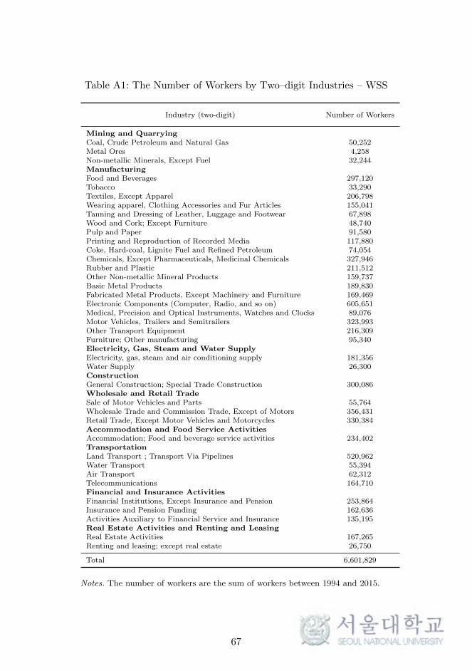
Table A1: The Number of Workers by Two–digit Industries – WSS

Industry (two-digit) Number of Workers

Mining and QuarryingCoal, Crude Petroleum and Natural Gas 50,252Metal Ores 4,258Non-metallic Minerals, Except Fuel 32,244ManufacturingFood and Beverages 297,120Tobacco 33,290Textiles, Except Apparel 206,798Wearing apparel, Clothing Accessories and Fur Articles 155,041Tanning and Dressing of Leather, Luggage and Footwear 67,898Wood and Cork; Except Furniture 48,740Pulp and Paper 91,580Printing and Reproduction of Recorded Media 117,880Coke, Hard-coal, Lignite Fuel and Refined Petroleum 74,054Chemicals, Except Pharmaceuticals, Medicinal Chemicals 327,946Rubber and Plastic 211,512Other Non-metallic Mineral Products 159,737Basic Metal Products 189,830Fabricated Metal Products, Except Machinery and Furniture 169,469Electronic Components (Computer, Radio, and so on) 605,651Medical, Precision and Optical Instruments, Watches and Clocks 89,076Motor Vehicles, Trailers and Semitrailers 323,993Other Transport Equipment 216,309Furniture; Other manufacturing 95,340Electricity, Gas, Steam and Water SupplyElectricity, gas, steam and air conditioning supply 181,356Water Supply 26,300ConstructionGeneral Construction; Special Trade Construction 300,086Wholesale and Retail TradeSale of Motor Vehicles and Parts 55,764Wholesale Trade and Commission Trade, Except of Motors 356,431Retail Trade, Except Motor Vehicles and Motorcycles 330,384Accommodation and Food Service ActivitiesAccommodation; Food and beverage service activities 234,402TransportationLand Transport ; Transport Via Pipelines 520,962Water Transport 55,394Air Transport 62,312Telecommunications 164,710Financial and Insurance ActivitiesFinancial Institutions, Except Insurance and Pension 253,864Insurance and Pension Funding 162,636Activities Auxiliary to Financial Service and Insurance 135,195Real Estate Activities and Renting and LeasingReal Estate Activities 167,265Renting and leasing; except real estate 26,750

Total 6,601,829

Notes. The number of workers are the sum of workers between 1994 and 2015.

67

Table A2: The Number of Establishments by Two–digit Industries –KED

Industry (two-digit)Number of

Establishments

Mining and quarryingCoal, Crude Petroleum and Natural Gas 175Metal Ores 58Non-metallic Minerals, Except Fuel 1,805ManufacturingFood and Beverages 26,982Tobacco 72Textiles, Except Apparel 20,187Wearing apparel, Clothing Accessories and Fur Articles 11,452Tanning and Dressing of Leather, Luggage and Footwear 4,219Wood and Cork; Except Furniture 5,126Pulp and Paper 9,065Printing and Reproduction of Recorded Media 10,662Coke, Hard-coal, Lignite Fuel and Refined Petroleum 1,194Chemicals, Except Pharmaceuticals, Medicinal Chemicals 32,143Rubber and Plastic 27,764Other Non-metallic Mineral Products 22,943Basic Metal Products 19,817Fabricated Metal Products, Except Machinery and Furniture 42,783Electronic Components (Computer, Radio, and so on) 41,900Medical, Precision and Optical Instruments, Watches and Clocks 18,549Motor Vehicles, Trailers and Semitrailers 26,976Other Transport Equipment 10,247Furniture; Other manufacturing 14,641Electricity, gas, steam and water supplyElectricity, gas, steam and air conditioning supply 1,534Water Supply 38ConstructionGeneral Construction; Special Trade Construction 181,493Wholesale and retail tradeSale of Motor Vehicles and Parts 10,809Wholesale Trade and Commission Trade, Except of Motors 201,671Retail Trade, Except Motor Vehicles and Motorcycles 16,724Accommodation and food service activitiesAccommodation; Food and beverage service activities 3,948TransportationLand Transport ; Transport Via Pipelines 13,054Water Transport 3,019Air Transport 172Telecommunications 1,700Financial and insurance activitiesFinancial Institutions, Except Insurance and Pension 126Insurance and Pension Funding 24Activities Auxiliary to Financial Service and Insurance 281Real estate activities and renting and leasingReal Estate Activities 12,298Renting and leasing; except real estate 2,377

Total 798,028

Notes. The number of establishments are the sum of establishments between 2000and 2015.

68

Table A3: The Estimation Results of the Augmented Mincer-type Wage Equation: Using Two–Digit Industry Dummies

Type of Wages Total Wage Fixed Wage

Dependent Variable: ln(wages) 1994 2002 2008 2015 1994 2002 2008 2015

Basic Variables

Years of schooling 0.041*** 0.056*** 0.077*** 0.077*** 0.038*** 0.055*** 0.075*** 0.067***

Experience 0.060*** 0.067*** 0.064*** 0.056*** 0.051*** 0.058*** 0.056*** 0.048***

Experience2 -0.001*** -0.001*** -0.001*** -0.001*** -0.001*** -0.001*** -0.001*** -0.001***

Union 0.114*** 0.260*** 0.274*** 0.299*** 0.025*** 0.120*** 0.107*** 0.127***

Interactions with Woman

Woman * Years of schooling -0.002*** 0.004*** 0.005*** 0.008*** -0.005*** 0.002*** 0.003*** 0.006***

Woman * Experience -0.038*** -0.037*** -0.036*** -0.029*** -0.033*** -0.032*** -0.031*** -0.025***

Woman * Experience2 0.001*** 0.001*** 0.001*** 0.000*** 0.001*** 0.001*** 0.000*** 0.000***

Woman * Union 0.079*** 0.039*** 0.112*** 0.007 0.074*** 0.045*** 0.122*** 0.039***

Occupation Dummies

Technicians and Associate Professionals -0.194*** -0.078*** 0.002 -0.341*** -0.247*** -0.080*** -0.004 -0.355***

Clerks -0.255*** -0.170*** -0.134*** -0.439*** -0.292*** -0.176*** -0.150*** -0.430***

Service Workers -0.298*** -0.313*** -0.347*** -0.616*** -0.345*** -0.281*** -0.326*** -0.572***

Sale Workers -0.379*** -0.298*** -0.287*** -0.599*** -0.390*** -0.266*** -0.279*** -0.576***

Skilled Agricultural, Forestry, and Fishery -0.452*** -0.586*** -0.522*** -0.750*** -0.462*** -0.509*** -0.470*** -0.723***

Craft and Related Trades Workers -0.428*** -0.348*** -0.338*** -0.589*** -0.430*** -0.326*** -0.328*** -0.589***

Plant, Machine Operators and Assemblers -0.465*** -0.398*** -0.439*** -0.666*** -0.459*** -0.375*** -0.421*** -0.645***

Elementary Occupations -0.656*** -0.556*** -0.598*** -0.780*** -0.652*** -0.508*** -0.542*** -0.741***

Constant -0.850*** -1.014*** -1.056*** -0.666*** -0.883*** -1.067*** -1.112*** -0.580***

Industry Dummies (two-digit) Yes Yes Yes Yes Yes Yes Yes Yes

R2 0.5964 0.5857 0.5201 0.52 0.5891 0.5554 0.5131 0.4952

N 300,567 240,099 349,056 318,538 300,567 240,099 349,056 318,538

Notes. This table shows the weighted regression results from the augmented Mincer type wage equation, described in equation (7) of section 4.1, using theWSS (Worker Structure Survey) data. Industry dummies at two–digit level are included in all models. Two types of (log real hourly) wages are used fordependent variables. Hourly fixed wage is regular wage per hour plus overtime wage per hour. Hourly total wage is hourly fixed wage plus hourly bonus.The bonus includes performance pay and non–production pay. The omitted occupation for estimation is Professionals. Standard errors are not reportedbecause most of them are less than 0.00. *** denotes significance at 1%.

69

Table A4: The Estimation Results of the Augmented Mincer-type Wage Equation: Using Industry–Size Dummies

Type of Wages Total Wage Fixed Wage

Independent Variable: ln(wages) 1994 2002 2008 2015 1994 2002 2008 2015

Basic Variables

Years of schooling 0.038*** 0.050*** 0.070*** 0.065*** 0.037*** 0.051*** 0.070*** 0.059***

Experience 0.058*** 0.065*** 0.064*** 0.057*** 0.050*** 0.057*** 0.056*** 0.048***

Experience2 -0.001*** -0.001*** -0.001*** -0.001*** -0.001*** -0.001*** -0.001*** -0.001***

Union 0.020*** 0.128*** 0.117*** 0.134*** -0.012*** 0.049*** 0.013*** 0.033***

Interactions with Woman

Woman * Years of schooling -0.005*** 0.002*** 0.002*** 0.004*** -0.007*** 0.001 0.001*** 0.004***

Woman * Experience -0.034*** -0.034*** -0.030*** -0.025*** -0.030*** -0.031*** -0.027*** -0.023***

Woman * Experience2 0.001*** 0.001*** 0.000*** 0.000*** 0.001*** 0.000*** 0.000*** 0.000***

Woman * Union 0.093*** 0.060*** 0.152*** 0.056*** 0.087*** 0.063*** 0.148*** 0.065***

Occupation Dummies

Technicians and Associate Professionals -0.254*** -0.066*** 0.047*** -0.347*** -0.276*** -0.071*** 0.022*** -0.351***

Clerks -0.286*** -0.147*** -0.085*** -0.394*** -0.311*** -0.161*** -0.120*** -0.395***

Service Workers -0.316*** -0.309*** -0.315*** -0.600*** -0.351*** -0.276*** -0.308*** -0.570***

Sale Workers -0.402*** -0.265*** -0.237*** -0.527*** -0.397*** -0.243*** -0.252*** -0.521***

Skilled Agricultural, Forestry, and Fishery -0.490*** -0.564*** -0.500*** -0.691*** -0.482*** -0.501*** -0.450*** -0.673***

Craft and Related Trades Workers -0.451*** -0.338*** -0.277*** -0.565*** -0.441*** -0.317*** -0.290*** -0.564***

Plant, Machine Operators and Assemblers -0.484*** -0.388*** -0.385*** -0.624*** -0.463*** -0.365*** -0.388*** -0.612***

Elementary Occupations -0.681*** -0.535*** -0.535*** -0.745*** -0.660*** -0.497*** -0.504*** -0.712***

Constant -0.736*** -0.885*** -0.979*** -0.502*** -0.831*** -0.987*** -1.054*** -0.483***

Industry–Size Dummies Yes Yes Yes Yes Yes Yes Yes Yes

R2 0.6328 0.6284 0.6089 0.6292 0.6121 0.5844 0.5612 0.5622

N 300,567 240,099 349,056 318,538 300,567 240,099 349,056 318,538

Notes. This table shows the weighted regression results from the augmented Mincer type wage equation, described in equation (7) of section 4.1, using theWSS (Worker Structure Survey) data. Industry–size group dummies at two–digit level and five categories (10–29, 30–99, 100–299, 300–499, and 500+) areincluded in all models. Two types of (log real hourly) wages are used for dependent variables. Hourly fixed wage is regular wage per hour plus overtimewage per hour. Hourly total wage is hourly fixed wage plus hourly bonus. The bonus includes performance pay and non–production pay. The omittedoccupation for estimation is Professionals. Standard errors are not reported because most of them are less than 0.00. *** denotes significance at 1%.

70

Table A5: The Estimated Group Wage Premiums (Total Wage, Year=1994)

IndustrySize Categories

10–29 30–99 100–299 300–499 500+

Mining and Quarrying

Coal, Crude Petroleum and Natural Gas -0.1401 0.0480 0.1290 0.0481 0.4139

Metal Ores -0.2625 0.0376 -0.0249 - -

Non-metallic Minerals, Except Fuel -0.0172 0.0160 0.0753 0.1665 -

Manufacturing

Food and Beverages -0.0934 -0.1891 -0.0324 -0.0821 -0.0601

Tobacco -0.0162 - 0.1391 - 0.4211

Textiles, Except Apparel -0.1673 -0.0923 -0.1421 -0.0937 -0.0212

Wearing apparel, Clothing Accessories and Fur Articles -0.1223 -0.1270 -0.1672 -0.2397 -0.0163

Tanning and Dressing of Leather, Luggage and Footwear -0.2276 -0.1595 -0.1992 -0.1330 -0.3104

Wood and Cork; Except Furniture 0.0384 -0.1268 -0.1214 -0.1842 -0.0139

Pulp and Paper -0.1568 -0.1803 0.1287 0.0888 0.0898

Printing and Reproduction of Recorded Media -0.1193 -0.2477 -0.1282 0.2114 0.2029

Coke, Hard-coal, Lignite Fuel and Refined Petroleum -0.0915 0.1612 0.2826 0.3833 0.5659

Chemicals, except pharmaceuticals, medicinal chemicals -0.1125 -0.1274 0.1322 0.1522 0.2027

Rubber and Plastic -0.1468 -0.0819 0.0733 0.0352 0.0150

Other Non-metallic Mineral Products -0.2284 -0.1378 -0.0614 0.0567 0.1849

Basic Metal Products -0.1112 -0.1114 -0.0706 -0.0183 0.2094

Fabricated Metal Products, Except Machinery and Furniture -0.0971 -0.1173 -0.0582 0.0527 0.2450

Electronic Components (Computer, Radio, and so on) -0.2579 -0.2140 -0.0698 0.0081 0.2086

Medical, Precision, Optical Instruments, Watches -0.0820 -0.1458 0.0854 0.0757 0.0588

Motor Vehicles, Trailers and Semitrailers -0.1963 0.0067 0.0665 -0.0508 0.2044

Other Transport Equipment -0.0653 -0.0248 0.0673 -0.1136 0.3047

Furniture; Other manufacturing -0.1896 -0.2073 -0.1485 -0.1125 -0.0966

Notes. This table shows the group wage premiums estimated by the wage equation (7) using the WSS data at the industry–size level.

71

Table A5–1: The Estimated Group Wage Premiums (Total Wage, Year=1994)

IndustrySize Categories

10–29 30–99 100–299 300–499 500+

Electricity, gas, steam and water supply

Electricity, gas, steam and air conditioning supply 0.0550 0.1047 0.1892 0.2259 0.1552

Water Supply - - - - 0.1941

Construction

General Construction; Special Trade Construction -0.0073 0.0174 0.0939 0.1273 0.2223

Wholesale and retail trade

Sale of Motor Vehicles and Parts -0.0888 -0.0355 0.1160 - 0.2460

Wholesale Trade and Commission Trade, Except of Motors -0.0431 -0.0621 0.1972 0.0135 0.2358

Retail Trade, Except Motor Vehicles and Motorcycles -0.1359 0.0013 -0.0780 0.0129 0.1415

Accommodation and food service activities

Accommodation; Food and beverage service activities -0.2049 -0.1400 -0.0241 -0.0229 0.2306

Transportation

Land Transport ; Transport Via Pipelines -0.3887 -0.2099 -0.2121 -0.1105 -0.1126

Water Transport -0.1327 0.1207 -0.0261 0.0660 0.1616

Air Transport -0.0002 0.1187 0.1139 - 0.4693

Telecommunications 0.2088 0.2061 0.3022 0.1918 0.3567

Financial and insurance activities

Financial Institutions, Except Insurance and Pension Funding 0.3236 0.2501 0.3417 0.6187 0.5220

Insurance and Pension Funding 0.2921 0.2352 0.4446 0.2645 0.2699

Activities Auxiliary to Financial Service and Insurance 0.3961 0.3155 0.3454 0.5046 0.5690

Real estate activities and renting and leasing

Real Estate Activities -0.3098 -0.3153 -0.0100 -0.1467 -0.2463

Renting and leasing; except real estate 0.1016 0.0005 0.3920 0.2879 0.9441

Notes. This table shows the group wage premiums estimated by the wage equation (7) using the WSS data at the industry–size level.

72

Table A6: The Estimated Group Wage Premiums (Total Wage, Year=2015)

IndustrySize Categories

10–29 30–99 100–299 300–499 500+

Mining and Quarrying

Coal, Crude Petroleum and Natural Gas - 0.4762 0.3814 0.4704 0.4851

Metal Ores -0.4855 -0.1592 - - -

Non-metallic Minerals, Except Fuel -0.2032 -0.0578 - - -

Manufacturing

Food and Beverages -0.2972 -0.1460 -0.0802 0.1485 -0.0560

Tobacco - 0.0237 0.3122 0.0943 0.4474

Textiles, Except Apparel -0.2626 -0.3062 -0.1620 0.0099 0.1247

Wearing apparel, Clothing Accessories and Fur Articles -0.2601 -0.2156 -0.1746 0.0826 0.2730

Tanning and Dressing of Leather, Luggage and Footwear -0.1807 -0.3136 -0.1923 - -

Wood and Cork; Except Furniture -0.2686 -0.2715 -0.0795 0.1866 -0.2152

Pulp and Paper -0.1597 -0.1504 0.0660 0.2532 0.4378

Printing and Reproduction of Recorded Media -0.1566 -0.0583 -0.2215 - -

Coke, Hard-coal, Lignite Fuel and Refined Petroleum -0.0998 -0.0018 0.4285 - 0.5800

Chemicals, except pharmaceuticals, medicinal chemicals -0.1345 -0.0382 0.1728 0.1481 0.2811

Rubber and Plastic -0.2360 -0.1530 -0.0601 0.1089 0.1858

Other Non-metallic Mineral Products -0.2230 -0.1235 -0.0360 0.1199 0.5302

Basic Metal Products -0.1684 -0.1401 0.0900 -0.1640 0.2951

Fabricated Metal Products, Except Machinery and Furniture -0.2041 -0.1640 -0.0893 0.0221 0.3540

Electronic Components (Computer, Radio, and so on) -0.1693 -0.0991 -0.1472 0.2233 0.6892

Medical, Precision, Optical Instruments, Watches -0.0869 -0.1289 -0.0620 0.1394 0.2278

Motor Vehicles, Trailers and Semitrailers -0.2291 -0.1789 -0.0217 0.0437 0.3670

Other Transport Equipment -0.1795 -0.1301 -0.1433 0.1487 0.3528

Furniture; Other manufacturing -0.2818 -0.1228 -0.0812 0.2630 0.6039

Notes. This table shows the group wage premiums estimated by the wage equation (7) using the WSS data at the industry–size level.

73

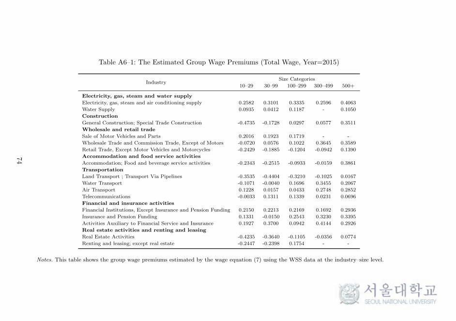
Table A6–1: The Estimated Group Wage Premiums (Total Wage, Year=2015)

IndustrySize Categories

10–29 30–99 100–299 300–499 500+

Electricity, gas, steam and water supply

Electricity, gas, steam and air conditioning supply 0.2582 0.3101 0.3335 0.2596 0.4063

Water Supply 0.0935 0.0412 0.1187 - 0.1050

Construction

General Construction; Special Trade Construction -0.4735 -0.1728 0.0297 0.0577 0.3511

Wholesale and retail trade

Sale of Motor Vehicles and Parts 0.2016 0.1923 0.1719 - -

Wholesale Trade and Commission Trade, Except of Motors -0.0720 0.0576 0.1022 0.3645 0.3589

Retail Trade, Except Motor Vehicles and Motorcycles -0.2429 -0.1885 -0.1204 -0.0942 0.1390

Accommodation and food service activities

Accommodation; Food and beverage service activities -0.2343 -0.2515 -0.0933 -0.0159 0.3861

Transportation

Land Transport ; Transport Via Pipelines -0.3535 -0.4404 -0.3210 -0.1025 0.0167

Water Transport -0.1071 -0.0040 0.1696 0.3455 0.2067

Air Transport 0.1228 0.0157 0.0433 0.2748 0.2852

Telecommunications -0.0033 0.1311 0.1339 0.0231 0.0696

Financial and insurance activities

Financial Institutions, Except Insurance and Pension Funding 0.2150 0.2213 0.2169 0.1692 0.2936

Insurance and Pension Funding 0.1331 -0.0150 0.2543 0.3230 0.3395

Activities Auxiliary to Financial Service and Insurance 0.1927 0.3700 0.0942 0.4144 0.2926

Real estate activities and renting and leasing

Real Estate Activities -0.4235 -0.3640 -0.1105 -0.0356 0.0774

Renting and leasing; except real estate -0.2447 -0.2398 0.1754 - -

Notes. This table shows the group wage premiums estimated by the wage equation (7) using the WSS data at the industry–size level.

74

Table A7: The Estimated Group Wage Premiums (Fixed Wage, Year=1994)

IndustrySize Categories

10–29 30–99 100–299 300–499 500+

Mining and Quarrying

Coal, Crude Petroleum and Natural Gas -0.0930 0.1644 0.1334 0.1107 0.4247

Metal Ores -0.1753 0.1636 0.0198 - -

Non-metallic Minerals, Except Fuel 0.0833 0.0656 0.0244 -0.0252 -

Manufacturing

Food and Beverages -0.0250 -0.1714 -0.0860 -0.0936 -0.1084

Tobacco -0.0737 - 0.1178 - 0.3193

Textiles, Except Apparel -0.0754 -0.0444 -0.0986 -0.0865 -0.0747

Wearing apparel, Clothing Accessories and Fur Articles -0.0201 -0.0512 -0.1463 -0.2344 -0.0409

Tanning and Dressing of Leather, Luggage and Footwear -0.0914 -0.0898 -0.1688 -0.1510 -0.3172

Wood and Cork; Except Furniture -0.0155 -0.0202 -0.1212 -0.1911 -0.0567

Pulp and Paper -0.1098 -0.0998 0.0793 -0.0342 0.0037

Printing and Reproduction of Recorded Media -0.0015 -0.1536 -0.0632 0.1103 0.1203

Coke, Hard-coal, Lignite Fuel and Refined Petroleum -0.0878 0.1264 0.1759 0.2231 0.3772

Chemicals, except pharmaceuticals, medicinal chemicals -0.0521 -0.0904 0.0553 0.0758 0.0966

Rubber and Plastic -0.0540 -0.0362 0.0381 -0.0119 -0.0471

Other Non-metallic Mineral Products -0.1497 -0.0970 -0.0976 -0.0229 0.0736

Basic Metal Products -0.0638 -0.0737 -0.0952 -0.0939 0.0663

Fabricated Metal Products, Except Machinery and Furniture 0.0064 -0.0658 -0.0717 0.0210 0.1651

Electronic Components (Computer, Radio, and so on) -0.2095 -0.1625 -0.0801 -0.0499 0.0952

Medical, Precision, Optical Instruments, Watches 0.0521 -0.1098 0.0154 0.0086 -0.0537

Motor Vehicles, Trailers and Semitrailers -0.0852 0.0175 0.0141 -0.0619 0.0623

Other Transport Equipment 0.0348 0.0711 0.0205 -0.1665 0.1814

Furniture; Other manufacturing -0.1567 -0.1575 -0.1228 -0.1390 -0.1263

Notes. This table shows the group wage premiums estimated by the wage equation (7) using the WSS data at the industry–size level.

75

Table A7–1: The Estimated Group Wage Premiums (Fixed Wage, Year=1994)

IndustrySize Categories

10–29 30–99 100–299 300–499 500+

Electricity, gas, steam and water supply

Electricity, gas, steam and air conditioning supply 0.0033 0.0959 0.1437 0.0978 0.1624

Water Supply - - - - 0.1083

Construction

General Construction; Special Trade Construction 0.0894 0.0843 0.0892 0.1152 0.1656

Wholesale and retail trade

Sale of Motor Vehicles and Parts -0.0044 0.0426 -0.0153 - 0.0771

Wholesale Trade and Commission Trade, Except of Motors -0.0058 -0.0240 0.1381 -0.0354 0.1019

Retail Trade, Except Motor Vehicles and Motorcycles -0.0808 0.0028 -0.0498 -0.0405 0.0377

Accommodation and food service activities

Accommodation; Food and beverage service activities -0.1018 -0.0506 0.0433 -0.0301 0.1610

Transportation

Land Transport ; Transport Via Pipelines -0.2297 -0.1005 -0.1257 -0.0364 -0.0580

Water Transport -0.0708 0.0646 -0.0625 0.0522 0.0923

Air Transport 0.0151 0.0851 0.0867 - 0.4281

Telecommunications 0.2401 0.1769 0.2373 0.1258 0.2832

Financial and insurance activities

Financial Institutions, Except Insurance and Pension Funding 0.2321 0.1248 0.2285 0.5331 0.4119

Insurance and Pension Funding 0.2367 0.1368 0.3215 0.1904 0.1512

Activities Auxiliary to Financial Service and Insurance 0.2681 0.1987 0.2561 0.3690 0.4669

Real estate activities and renting and leasing

Real Estate Activities -0.2824 -0.2786 -0.0204 -0.1602 -0.2073

Renting and leasing; except real estate 0.0905 0.0865 0.3734 0.1893 0.8666

Notes. This table shows the group wage premiums estimated by the wage equation (7) using the WSS data at the industry–size level.

76

Table A8: The Estimated Group Wage Premiums (Fixed Wage, Year=2015)

IndustrySize Categories

10–29 30–99 100–299 300–499 500+

Mining and Quarrying

Coal, Crude Petroleum and Natural Gas - 0.3943 0.3969 0.5529 0.4293

Metal Ores -0.3586 -0.1027 - - -

Non-metallic Minerals, Except Fuel -0.1362 -0.0224 - - -

Manufacturing

Food and Beverages -0.2010 -0.0976 -0.0825 0.1088 -0.0668

Tobacco - -0.0594 0.2937 0.3194 0.4174

Textiles, Except Apparel -0.1659 -0.2314 -0.0719 0.1082 -0.0141

Wearing apparel, Clothing Accessories and Fur Articles -0.1386 -0.1004 -0.1314 0.1715 0.3058

Tanning and Dressing of Leather, Luggage and Footwear -0.0839 -0.2009 -0.1693 - -

Wood and Cork; Except Furniture -0.1833 -0.2155 0.0070 0.2279 -0.1931

Pulp and Paper -0.0833 -0.1055 -0.0505 0.0899 0.1807

Printing and Reproduction of Recorded Media -0.0366 0.0315 -0.1619 - -

Coke, Hard-coal, Lignite Fuel and Refined Petroleum -0.0140 -0.0704 0.1402 - 0.3881

Chemicals, except pharmaceuticals, medicinal chemicals -0.0384 -0.0424 0.0994 0.1531 0.2016

Rubber and Plastic -0.1470 -0.1192 -0.0707 0.0473 0.0201

Other Non-metallic Mineral Products -0.1328 -0.0963 -0.0873 -0.0248 0.2469

Basic Metal Products -0.1357 -0.1836 -0.0321 -0.1865 0.0855

Fabricated Metal Products, Except Machinery and Furniture -0.1304 -0.1064 -0.0882 -0.0726 0.2115

Electronic Components (Computer, Radio, and so on) -0.0683 -0.0305 -0.1112 0.0688 0.4251

Medical, Precision, Optical Instruments, Watches -0.0433 -0.0362 0.0669 0.1485 0.1428

Motor Vehicles, Trailers and Semitrailers -0.1548 -0.1439 -0.0486 -0.0474 0.1487

Other Transport Equipment -0.0842 -0.0748 -0.1343 0.1258 0.1563

Furniture; Other manufacturing -0.1690 -0.0862 -0.1482 0.1590 0.3163

Notes. This table shows the group wage premiums estimated by the wage equation (7) using the WSS data at the industry–size level.

77

Table A8-1: The Estimated Group Wage Premiums (Fixed Wage, Year=2015)

IndustrySize Categories

10–29 30–99 100–299 300–499 500+

Electricity, gas, steam and water supply

Electricity, gas, steam and air conditioning supply 0.3132 0.3205 0.2557 0.2179 0.4187

Water Supply 0.1764 0.1372 0.1471 - 0.1188

Construction

General Construction; Special Trade Construction -0.3476 -0.0873 0.0741 0.1288 0.3966

Wholesale and retail trade

Sale of Motor Vehicles and Parts -0.0696 0.2289 0.1994 - -

Wholesale Trade and Commission Trade, Except of Motors -0.0167 0.0917 0.1416 0.3132 0.2537

Retail Trade, Except Motor Vehicles and Motorcycles -0.1719 -0.1516 -0.1173 -0.1003 0.1280

Accommodation and food service activities

Accommodation; Food and beverage service activities -0.1474 -0.1757 -0.0769 -0.2176 0.0852

Transportation

Land Transport ; Transport Via Pipelines -0.2441 -0.3147 -0.2143 -0.0422 0.1130

Water Transport -0.0649 0.0798 0.1379 0.5235 0.3572

Air Transport 0.1202 -0.0423 -0.1369 -0.0405 0.2555

Telecommunications 0.0621 0.0596 0.1437 0.0228 0.1264

Financial and insurance activities

Financial Institutions, Except Insurance and Pension Funding 0.1339 0.1713 0.2410 0.1952 0.1949

Insurance and Pension Funding 0.1007 0.0343 0.2864 0.2741 0.3156

Activities Auxiliary to Financial Service and Insurance 0.1014 0.2958 0.0433 0.2574 0.2951

Real estate activities and renting and leasing

Real Estate Activities -0.3157 -0.2714 -0.0349 0.0499 0.1563

Renting and leasing; except real estate -0.1311 -0.1568 0.2659 - -

Notes. This table shows the group wage premiums estimated by the wage equation (7) using the WSS data at the industry–size level.

78

Figure A1: The Comparison of Variances of (log) Hourly TotalWages between Original Data and Sample Data

.1.2

.3.4

.5

Variance o

f (log)

Hourly T

ota

l W

age

1994 1996 1998 2000 2002 2004 2006 2008 2010 2012 2014

Original Data Sample

Notes. Original data means the data before the manipulation of industry.The number of observations and industries of the original data between1994 and 2015 are 10,612,699 and 83, respectively. Sample means the dataafter the manipulation of industry. The number of observations and in-dustries of the sample data in the same period are 6,601,829 and 37, re-spectively. Although about a half of industries and 40% of workers in theoriginal data are deleted by sample restriction, the trends in variances oflog real hourly total wage are similar.

79

Figure A2: The Estimated Results of Quantile Regression by Pe-riods (Fixed Wages)

0.0

3.0

6.0

9

La

bo

r P

rod

uctivity

0 .1 .2 .3 .4 .5 .6 .7 .8 .9 1

0.0

3.0

6.0

9

Ca

pita

l−to

−L

ab

or

Ra

tio

0 .1 .2 .3 .4 .5 .6 .7 .8 .9 1

−.2

0.2

.4.6

Alte

rna

tive

Wa

ge

s

0 .1 .2 .3 .4 .5 .6 .7 .8 .9 1

.7.9

1.1

1.3

1.5

Wo

rke

r C

ha

racte

ristics

0 .1 .2 .3 .4 .5 .6 .7 .8 .9 1

Period 1(2002−2008) Period 2(2009−2015)

Notes. This figure shows the coefficient estimates, β, using equation (18). Theregressions are implemented for every 2.5% wage quantiles. X-axis means 2.5%quantiles of the average wages at the industry–size level.

80

국문초록

사업체 규모, 산업과 임금 불평등:

보너스와 수익 배분의 역할을 중심으로

본 논문에서는 고용노동부의 임금구조부문 자료(WSS), 한국노동패

널(KLIPS) 및 기업 재무제표 자료(KED)를 이용하여 기업 측면의 요인

이 우리나라 임금 불평등에 미친 영향에 대해 다룬다. 분석기간은 1994

년부터 2015년까지다.

본 논문에서 밝히고자 하는 것은 크게 두 가지다. 먼저, 산업과 기

업규모 간 임금격차가 노동자의 임금 불평등에 미친 영향을 분석한다.

대표성을 가지고 있는 고용노동부 자료를 주로 이용하되, 시간에 따라

변하지않는노동자들의특성을통제하기위해한국노동패널을보조적으

로 활용한다. 다음으로, 기업 재무제표 자료와 고용노동부 임금구조부문

자료를연계하여산업및기업규모간임금격차의원인을분석한다.산업

및 기업규모 간 노동생산성의 차이, 수익 공유의 정도 차이, 자본 의존도

차이, 자본 의존에 대한 보상 차이 등이 주요 관심 변수다.

이러한 두 가지 주제를 연구함에 있어 주요 변수인 임금은 고정임

금과 총임금 두 가지 종류를 고려한다. 총임금에는 고정임금에 더하여

보너스가 포함되며, 보너스는 성과급과 복지 차원의 비생산임금(non-

production pay)의 합으로 정의한다. Lemieux et al. (2009)은 미국 노

동시장에서 성과급이 임금 불평등에 부정적인 영향을 미친다고 보고하

였는데 이러한 결과가 우리나라에도 적용되는지, 아니라면 미국과 우리

81

나라의 차이점은 무엇인지를 파악하는 것이 두 가지 종류의 임금을 함께

관찰하는 이유다.

주요결과는다음과같다.첫째, 1994년이후우리나라임금불평등의

지속적인 악화는 산업 간 임금격차보다 기업규모 간 임금격차에 더 큰

영향을 받았다. 임금방정식을 추정한 후 임금의 분산을 집단 내 분산과

집단 간 분산으로 분해하여 보면 산업 간 임금격차는 임금 불평등 상

승분의 11.33%를 설명하는 데에 그친 반면, 산업과 기업규모를 동시에

고려할 경우 이들 간 임금격차는 임금 불평등 상승분의 44.03%를 설명

하는 것으로 나타났다. 이는 기업규모가 산업 대비 임금 불평등에 더 큰

영향을 미치고 있음을 보여준다. 산업 및 기업규모 간 노동자들의 인적

자본차이(학력,경력등)는임금불평등의절대적인수준에는큰영향을

미쳤으나, 추이의 변화에는 영향력이 크지 않았다.

둘째, 산업 및 기업규모 간 임금격차의 상승은 고정임금 뿐 아니라

보너스의 차이에도 큰 영향을 받은 것으로 나타났다. 고정임금만을 고

려하면 산업-규모 간 임금격차는 임금 불평등 상승분의 29.35%만을 설

명하는 데에 그쳤으며, 이는 앞에서 말한 44.03% 보다 약 14.68%p 낮은

수치다. 또한 보너스는 산업-규모 내 임금격차보다 산업-규모 간 임금격

차에 더 큰 영향을 미쳤는데, 이는 미국의 사례를 분석한 Lemieux et al.

(2009)과 다른 결과다. 이는 성과급의 역할이 미국과 우리나라에서 다를

가능성을 제기한다.

셋째, 노동자들의 관측되지 않는 속성이 산업-규모 간 임금격차 추이

에 미친 영향은 크지 않았다. 한국노동패널을 이용하여 노동자의 고정

효과를 통제한 후 임금의 집단 간 분산과 집단 내 분산 추이를 관찰한

82

결과, 노동자들의 미관측 속성은 임금 불평등 수준에 매우 큰 영향을 미

쳤으나 추이에는 영향을 미치지 못하였다. 반면 횡단면 자료에서 관측된

산업및기업규모간임금격차가임금불평등추이에미친영향력은크게

달라지지 않았다. 횡단면 자료와 종단면 자료를 함께 이용하여 도출된

위의결과들은기업규모간임금및보너스격차가 1994년이후우리나라

임금 불평등을 악화시킨 주요인이라는 것을 보여준다.

넷째, 고용노동부 임금구조부문 자료와 기업 재무제표 자료를 연계

하여 산업-규모 간 임금격차의 원인을 분석한 결과, 이는 산업-규모 간

수익 공유 정도의 차이와 자본 의존에 대한 보상 차이에 큰 영향을 받

은 것으로 나타났다. Machado and Mata (2005)의 방법론을 이용하여

반사실적 분포(counterfactual distribution)를 추정하였는데, 산업-규모

간 수익 공유 파라미터(rent-sharing parameter)의 차이는 산업-규모 평

균임금의 분산을 0.131에서 0.1879까지 상승시켰으며, 자본 의존에 대한

보상 차이의 경우 산업-규모 평균임금의 분산을 0.1808까지 상승시킨 것

으로 추정되었다. 이는 산업-규모 간 이질적인 수익 공유와 자본 의존에

대한 보상이 임금 불평등에 큰 영향력을 행사하고 있음을 시사한다.

다섯째, 위에서 보인 결과들은 보너스가 임금에 포함될 때에만 유의

한 것으로 나타났다. 고정임금만을 가지고 동일한 분석을 진행한 결과

산업-규모 간 이익 공유의 차이와 자본 의존에 대한 보상 차이가 유의미

하지 않았으며, 이는 기업들이 보너스를 수익 공유 및 자본 의존에 대한

보상 수단으로 활용하고 있음을 보여준다.

본 연구에서는 우리나라 임금 불평등이 산업 및 기업규모 간 이질적

인 특성에 상당 부분 영향을 받고 있다는 결과를 보였으나, 이들이 왜

83

이질적인지는 다루지 못하였다. 우리나라 임금 불평등에 대한 심도 깊은

이해를 위해서는 기업 간 노동생산성의 격차가 어디에서 비롯되는지, 노

동생산성이 유사한 기업일지라도 왜 어떤 기업은 다른 기업 대비 수익을

노동자들에게 더 많이 분배하는지 등의 질문들에 대한 해답을 찾아 나

가야 할 것이다. 또한 본 논문에서 보인 기업규모 간 임금 불평등 악화가

대기업과 중소기업 간의 관계(원하청 관계, 수직적 상하관계 등)에서 비

롯되는 것은 아닌지 점검해 볼 필요가 있다.

주요어: 임금 불평등, 보너스, 사업체 규모, 산업, 노동생산성,

자본-노동 비율, 수익 공유 행동

학 번: 2014–30968

84