Disagreement is Bad News

Bryan Lim∗

Department of FinanceUniversity of Melbourne

November 3, 2017

Abstract

I investigate whether the documented relationship between disagreement andfuture returns is driven by negative correlation between disagreement and funda-mentals (unexpected earnings). I posit a model in which negative skewness in fun-damentals interacts with heterogeneous weights in adopting new signals, generatinghigher disagreement when the underlying fundamentals are low. Across a numberof empirical tests, I find robust evidence of the model’s predictions. Conditioningon the realized fundamental, the ability for disagreement to predict future returnsis virtually completely attenuated. Additionally, consistent with my model and in-consistent with prior hypotheses, I find the negative correlation between monthlyanalyst dispersion and next-month returns is driven by a combination of positiveserial correlation in dispersion and negative correlation between returns and con-temporaneous dispersion.

∗e-mail: blim@unimelb.edu.au

1

Financial markets aggregate differential information across investors, and a key con-

sideration in this process is the nature and the role of disagreement. What does it mean

for investors to disagree, and how does that disagreement translate into prices? The lit-

erature has largely investigated two hypotheses. The first, as put forth by papers like

Varian (1985) and David (2008), posits that disagreement generates risk for which in-

vestors must be compensated. According to this story, high disagreement pushes down

prices and pushes up expected returns. Carlin, Longstaff, and Matoba (2014) examine

the market for mortgage-backed securities and find results consistent with this hypothe-

sis. The second hypothesis follows Miller (1977), who observed that when short selling is

constrained, securities with higher disagreement should have higher prices, all else equal.

Using the dispersion of analyst forecasts to measure disagreement in a given month, Di-

ether, Malloy, and Scherbina (2002; henceforth DMS) examine whether returns in the

subsequent month are lower for stocks with high disagreement relative to those with low

disagreement. By the Miller logic, high disagreement should be correlated with abnor-

mally high contemporaneous prices which cannot be arbitraged down due to constraints

on short selling. Assuming high disagreement tends to dissipate, the price will tend to

fall, so we should observe lower subsequent-month returns. Indeed, this is exactly what

DMS find: high disagreement in month t is correlated with low returns in month t+ 1.

My paper revisits the relationship between disagreement and prices for equities and

considers an alternate possibility: that disagreement predicts future fundamentals and the

consequent returns in a way that is unrelated to the risk- or overpricing-based mechanisms.

Where the existing has largely treated disagreement as exogenous, I hypothesize that it

is instead an artifact of the unobserved financial state of the firm. According to my

hypothesis, firms with poor (unannounced) fundamentals have higher pre-announcement

disagreement. High disagreement consequently precedes low fundamentals, which in turn

generate low returns.

In empirical tests across sixteen combinations of measures of disagreement, short-sale

constraints, and fundamentals, where the fundamental of interest is quarterly earnings

2

per share, I find compelling evidence that 1) disagreement predicts the unexpected and

unpriced component in fundamentals; and 2) controlling for the realized fundamental,

virtually all of the cross-sectional variation in future returns previously attributed to

disagreement via a Miller-overpricing story disappears. Additionally, I find that when

disagreement is measured by the monthly dispersion of analyst forecasts as in DMS, 3)

increasing (decreasing) disagreement is matched by a contemporaneous decrease (increase)

in the security’s price; and 4) high (low) disagreement in months t and t+ 1 is correlated

with low (high) returns in month t + 1. While (3) is consistent with a risk-based story,

(4) is not, since holding disagreement – i.e., risk – constant, the expected return should

be positively correlated with the level of disagreement. Moreover, both (3) and (4) run

counter to a Miller story. (3) and (4) underlie the ultimate dynamic: 5) disagreement is

serially correlated, and the realized return for a given month is negatively correlated with

the contemporaneous disagreement.

I frame the results with a stylized model which yields testable predictions regarding the

dynamics between disagreement, returns, and fundamentals. The model is based on two

building blocks. The first is agents’ heterogenous weighting of new versus old information.

The second is negative skewness in fundamentals, whereby positive fundamentals are

more likely than negative fundamentals but are smaller in magnitude. When positive

information arrives, it is relatively small in magnitude, so variation in agents’ weights in

updating their priors generates relatively small disagreement among them. When negative

information arrives, it is relatively large in magnitude, so the equivalent variation in

weights generates relatively large disagreement among them. If prices reflect mean beliefs,

this skewness-based model predicts disagreement will be negatively correlated with the

contemporaneous return as well as the future realized fundamental and the associated

future return. Moreover, the correlation between disagreement and future returns will be

driven only by disagreement’s correlation with the fundamental. According to the model,

conditioning on the fundamental, disagreement is uncorrelated with future returns.

The skewness model yields predictions which separately identify it from the Miller

3

model. I take the two models’ respective predictions to the data via two lines of in-

quiry. The first builds upon Berkman, Dimitrov, Jain, Koch, and Tice (2009; henceforth

BDJKT), who apply the DMS analysis to earnings announcement returns. Under the

assumption that an earnings announcement – i.e., the revelation of the information about

which the disagreement exists – necessitates a reduction in disagreement, BDJKT examine

the differential announcement returns for stocks with high versus low pre-announcement

disagreement. Consistent with Miller, they find high-disagreement stocks have signifi-

cantly lower announcement returns than low-disagreement stocks. With an expanded

sample, I am able to replicate their results. Consistent with the skewness model, I addi-

tionally observe that high disagreement predicts low fundamentals and that conditional

on the fundamental, disagreement has no additional predictive power over future returns.

Crucially, these results hold across multiple specifications of disagreement, short-sale con-

straints, and fundamentals.

The second line of inquiry builds upon DMS. DMS test monthly returns versus prior

dispersion, and I extend the tests to include contemporaneous dispersion. Extrapola-

tion of a Miller overpricing mechanism to a dynamic setting predicts a negative correla-

tion between changes in disagreement and the corresponding contemporaneous returns.

Consistent with the skewness model and contrary to the overpricing model, I find that

contemporaneous disagreement drives the return and that the observed predictability of

returns from prior disagreement is due to serial correlation in disagreement.

Taken as a whole, my results can be distilled to a single basic conclusion: disagreement

is bad news. The implications of this are manifold. First, they provide a novel mechanism

by which disagreement predicts returns, alternative to the risk- and overpricing-based

hypotheses. Disagreement is driven by fundamentals, which mechanically generate the

observed future returns. Second, they raise questions for both behavioral-finance propo-

nents and their market-efficiency counterparts. For the former, are the results driven by

some sort of cognitive bias, and if so, why are they not arbitraged away? For the latter,

is there a way to reconcile disagreement’s predictive ability over the unpriced surprise in

4

fundamentals within a rational framework? Finally, the results potentially speak to both

the belief adjustment and, to a lesser extent, anchoring hypotheses in psychology.1 Insofar

as the mechanism in the skewness model describing the transformation of a public signal

into beliefs is correct, the observed joint time-series dynamics of disagreement, returns,

and fundamentals validates theories in which agents do not fully (rationally/optimally)

update their priors when new information arrives.

My primary contribution is to the literature on disagreement and information diffu-

sion. The innovation is the idea that observed disagreement is endogenously generated

by underlying fundamentals. Prior research has typically treated disagreement as a state

variable. Zhang (2006), for example, documents how information uncertainty (as mea-

sured by similar proxies as disagreement in my paper) contributes to market underreaction

to public news, and Cen, Wei, and Yang (2016) observe that the interaction between dis-

agreement and underreaction is informative about future returns. My results suggest that

the unrealized fundamental is the state variable, and disagreement is determined by the

state. Hong and Stein (1999) and Hong, Lim, and Stein (2000) connect momentum in

returns to the diffusion of information across participants. The latter empirically tests

a proposition in the former: that momentum strategies will be more effective on firms

with lower analyst coverage, since analysts propagate information flow. For low-analyst-

coverage stocks, bad news travels slower than good news, a result which the authors posit

is driven by the asymmetric incentives for low-coverage firm managers to reveal good ver-

sus bad news. My skewness model overlaps with asymmetric-incentives theory advanced

in Hong, Lim, and Stein (2000) and provides an explicit mechanism to tie news to disagree-

ment. In the context of sell-side analysts, Scherbina (2008) observes that fewer forecasts

are issued when the underlying state is bad, hypothesizing that career concerns incentivize

analysts not to issue negative forecasts. Her insights build upon Hong, Lim, and Stein

(2000), who argued that firm managers have asymmetric incentives to disseminate good

versus bad news. I demonstrate a parallel channel connecting disagreement to firm funda-

1See Hogarth and Einhorn (1992) for belief adjustment and Kahneman and Tversky (1975) for an-choring.

5

mentals and returns, one that does applies to a broader set of market participants besides

analysts. Crucially, my results hold for both analyst-based and market-based measures of

firm fundamentals, suggesting that analyst career concerns alone do not drive the results.

My paper also contributes to the dispersion anomaly documented in DMS. Since its

publication, several papers have investigated alternative explanations for the relationship

between analyst dispersion and future returns. Johnson (2004) observes that expected

returns for levered firms should decrease with idiosyncratic asset risk, so if disagreement

proxies for idiosyncratic risk, it follows that high disagreement should be correlated with

low future returns. Avramov, Chordia, Jostova, and Philipov (2009) demonstrate that

dispersion is negatively correlated with credit ratings, and the differential returns between

high and low analyst-dispersion firms is driven by differences in credit. My skewness model

complements these papers by providing a mechanism connecting fundamentals to observed

differences in analyst dispersion.

Finally, I contribute to the literature examining analyst bias and returns. Grinblatt,

Jostova, and Philipov (2017) demonstrate that the ex-post bias in analyst forecasts is

predictable, and for firms whose earnings are difficult to forecast, the predicted bias is

negatively correlated with future returns. They posit that when earnings are difficult to

forecast, market participants will rely more on analyst forecasts than when earnings are

easier to forecast, and this “pied piper” effect leads to the observed correlation between

difficulty of forecasting (e.g., high analyst dispersion) and future returns. Similarly, Veen-

man and Verwijmeren (forthcoming) argue that that analyst career incentives provide a

channel through which the observed relationship between dispersion, ex-post bias, and

returns can occur. The theory and results in my paper provide a complementary interpre-

tation of these results, whereby the forecasts of analysts reflect the beliefs of the investor

population at large. In this case, analyst bias is indicative of investor bias, a possibility

supported by my finding that disagreement is correlated with both future ex-post bias and

future standardized unexpected earnings, the latter an accounting measure which cannot

be affected by analysts.

6

The structure of the paper is as follows. Section 1 presents a theoretical model, which

is used to derive predictions that can be compared to those from Miller (1977). Section

2 details the construction of the data. In Section 3, I test the predictions using earnings

announcements. In Section 4, I test the predictions using monthly analyst dispersion.

Section 5 takes a deeper look at the disagreement measures. Section 6 concludes.

1 Theory and Predictions

In this section, I present a simple model connecting disagreement, fundamentals, and re-

turns. The model is heavily stylized, abstracting from considerations like investor utility

and markets clearing, in an attempt to convey the underlying mechanism as parsimo-

niously as possible. The model is purposefully limited in scope, having nothing to say,

for example, about the plausibility of agents with common priors disagreeing, as Aumann

(1976) described. What the model provides is a channel linking disagreement to both

fundamentals and returns that is distinct from Miller (1977).

1.1 The Model

I model a market for a single security over three periods: t ∈ {0, 1, 2}. Analysts are

trying to determine the value of the fundamental F , where F is realized at t = 2. I use

the term “analysts” here to keep the description consistent with my main empirical tests,

but fundamentally I am referring to all participants in the market. The distribution of F

is given by:

F =

∆ > 0 with probability p > 1/2

−K∆ < 0 with probability 1− p

where K > 1 and E[F ] = 0.

At time 0, the price of the security is P0, and all analysts have the same belief about

F : namely, that its expectation is 0.

At time 1, a public signal S = F + ε arrives, where ε is distributed with mean 0 and

7

σε > 0. Analyst n calculates her prediction xn of F as a weighted average of her prior

belief and S:

xn = λnS + (1− λn)0 = λnS

where λn ∈ (0, 1), µλ < 1, and σλ 6= 0. λn can be interpreted in multiple, non-mutually

exclusive ways. One interpretation is that it represents the ability of the analyst to process

the signal. High-ability analysts are able to process the signal faster than low-ability ones,

meaning they have higher λ. Another interpretation is that it represents the weight the

analyst places on new information when updating her priors. Lahiri and Sheng (2008) use

λ to represent the weight attached to prior beliefs when signals are normally distributed.

In the language of psychology, 1 − λ measures the analyst’s belief perseverance (e.g.,

Anderson, Lepper, and Ross, 1980; Ross, Lepper, and Hubbard, 1975; Lord, Ross, and

Lepper, 1979).

The condition that σλ 6= 0 means that there exists at least some variation across agents

in their respective abilities. Imagining this as a repeated game, it is not necessarily the

case that λn is fixed for analyst n in every market and every time period she participates.

λn can be thought of specific to a particular analyst for a particular security over a

particular period of time.

Analysts are atomistic and individually have no price impact. The time-1 price P1 is

the average expectation of the next-period price P2:

P1 = P0 +

∑N λnS

N= P0 + µλS

Disagreement at time 1 is measured as the standard deviation of analysts’ beliefs,

which is equivalent to the the signal S times the cross-sectional variation in λn:

D1 = σ(xn) = Sσλ

At time 2, F is revealed, and the price is P2 = P0+F . Figure 1 illustrates the timeline.

8

[Figure 1 about here]

1.2 Predictions

Conditioning on F , I derive expectations for disagreement and returns. By “expectations”,

I mean the expected observed average, conditional on the ex-post realization of F . An

equivalent interpretation is the expectation from the point of view of an omniscient but

passive observer. I note that the analysts’ expectations are not meaningful in this setting,

since their behavior is constrained by the assumptions of the model. For example, in the

cross-section of analysts, the average one-period expected return among them is 0 at both

time 0 and 1.

The conditional expectation of disagreement at time 1 is

E[D1|F ] = E[σ(λnS)|F ] = σ(λn(F + ε)) = σλ|F | (1)

assuming λn is uncorrelated with F and ε. The conditional expectations of the time-1

and 2 returns are, respectively,

E[R1|F ] =P0 + µλF − P0

P0

=µλF

P0

(2)

E[R2|F ] =P0 + F − (P0 + µλF

P0 + µλF=

(1− µλ)FP0 + µλF

(3)

Equations (1) to (3) tie disagreement and returns to realizations of F . Assuming that

the distribution of λn is equivalent across securities (and independent of the realization of

F ), when F is positive we should observe low disagreement at time 1 and positive returns

at times 1 and 2. When F is negative, we should observe relatively high disagreement at

time 1 and negative returns at times 1 and 2.

We can flip these relationships around. Low disagreement should be correlated with

positive contemporaneous returns and predict both positive future returns and fundamen-

tals. Similarly, high disagreement should be correlated with negative contemporaneous

9

returns and predict both negative future returns and fundamentals.

The disagreement result is given by Equation (1). Assuming the distribution of λ is

independent of F , then if F is negatively skewed, negative fundamentals should manifest

in higher disagreement. The return results – for time 2, in particular – are artifacts of

the mean λ being less than 1.

The model predictions are easily applied to the empirical setting in BDJKT, wherein

disagreement is measured just prior to an earnings announcement. To extend the model

to the monthly setting in DMS, the model can be respecified as ending at period T > 2.

From periods 1 to T − 1, the analyst updates her beliefs by placing weight λn on S and

1 − λn on her prior. As the current period t approaches T , her beliefs converge toward

the fundamental:

xn,t =t−1∑j=0

(1− λn)jλS

Two predictions can be derived from this setting. First, conditional on a single sig-

nal S, disagreement is serially correlated. Second, since changes in the ranked level of

disagreement can only occur with a new signal S, conditional on a change in ranked dis-

agreement returns are negatively correlated with contemporaneous disagreement but not

prior disagreement. To put this slightly differently: Controlling for serial correlation in

disagreement, returns are negatively correlated with contemporaneous disagreement and

uncorrelated with past disagreement.

1.3 Compared to Miller (1977)

The intuition in Miller (1977) has shaped the a considerable portion of the discussion on

disagreement. Here I detail the predictions that come from a Miller-style model applied

to the dynamic setting in the skewness-based model.

Miller models the market for a security as a downward-sloping demand curve in-

teracting with an inelastic supply curve. The steepness of the demand curve indicates

disagreement, and the x-intercept of the supply curve represents the degree to which

10

short-sales are constrained. In contrast to the skewness model, Miller makes no refer-

ence to fundamentals. The implicit assumption in DMS and BDJKT is that dispersion is

not correlated with fundamentals. Under this assumption, disagreement should predict

future returns even conditional on the realized fundamental. According to this reading

of Miller, amongst all stocks with (e.g.) high earnings surprises, those that had higher

pre-announcement disagreement should experience lower returns.

Extracting dynamic predictions from Miller’s static model requires making assump-

tions about how the supply and demand curves move. The assumptions I apply are con-

sistent with those implicit in prior literature. In a Miller setting, changes in disagreement

should manifest in changes in the slope of the demand curve. If:

1. Shifts in the supply curve are independent of changes to the demand curve, and

2. The point at which the demand curve pivots is both independent of the change in

the slope (i.e., changes in disagreement are uncorrelated with shifts in the demand

curve) and positioned to the right of the supply curve (i.e., the constraint is binding),

a number of straightforward predictions can be derived.

Figure 2 illustrates a Miller-style security market with two potential demand curves,

one corresponding to high disagreement (DH) and the other to low disagreement (DL).

When disagreement doesn’t change from t to t + 1, the demand curve remains in place,

and the average contemporaneous return rt+1 should be 0. When disagreement increases

(DL → DH), the average return should be positive. When disagreement decreases (DL →

DH), the average return should be negative.

[Figure 2 about here]

Table 1 lists the corresponding predictions from my skewness model and Miller (1977),

conditioning on some (potentially ex-post) observable. As noted previously, the expecta-

tion refers to the ex-post expected average. It does not refer to the ex-ante expectation of

the participating analysts. As the empirical analyses will use ranked measures of variables

11

rather than cardinal measures, in comparing the models’ predictions for a cross-section

of securities I’ll henceforth abandon signs and magnitudes and instead use the relative

terms “low” and “high”. Accordingly, the “<0”, “=0”, and “>0” notations in Table 1

are to be read as “low”, “average”, and “high”, respectively.

[Table 1 about here]

Panel A lists the predictions around earnings announcements. H1 states that condi-

tional on high pre-announcement disagreement, the skewness model predicts low funda-

mentals, while Miller’s model, by assumption, predicts average fundamentals (i.e., F = 0).

H2 states that conditional on the realized fundamental, the skewness model predicts that

the correlation between pre-announcement disagreement and the announcement return is

0. While this result is easily verified analytically (F is the only random variable), the intu-

ition is that disagreement affects prices only through fundamentals, so conditional on the

fundamental, cross-sectional variation in dispersion is uninformative about the announce-

ment return. By contrast, Miller’s model predicts the correlation between dispersion and

is negative, regardless of the realized fundamental.

Panel B lists the predictions regarding monthly disagreement. In the skewness model,

monthly disagreement is serially correlated (H3). Controlling for this serial correlation,

what drives the return in a given month is the contemporaneous analyst dispersion, not the

prior dispersion. the skewness model predicts high (low) dispersion is correlated with low

(high) contemporaneous returns (H4/A/B and H5/A/B). Miller’s model predicts that the

change in dispersion is positively correlated with the contemporaneous return but has no

prediction about the correlation between the level of dispersion and the contemporaneous

return.

2 Data Construction

The data come from standard sources. I/B/E/S provides analyst EPS forecasts and

monthly summaries. CRSP provides daily and monthly stock returns, prices, volumes,

12

and shares outstanding, as well as index returns. I use Compustat for earnings and

other corporate fundamentals. Institutional ownership is from Thomson Reuters 13f data.

Markit provides indicative short-sale fees. For all variables except short-sale fees, the

sample runs from 1985 to 2015. Tests involving short-sale fees are limited to a sample

from 2002 to 2015.

In Section 3, I follow BDJKT and examine (-1, +1) buy-and-hold abnormal returns

(BHAR) around quarterly earnings announcements. BHAR is calculated via a simple

market-adjusted model using the CRSP value-weighted index.

I calculate multiple measures of disagreement, following BDJKT. The first is the dis-

persion of analyst forecasts (ANADISP). For stock i in quarter t, the sample of forecasts

is the last EPS forecast for the quarter made by each analyst in the 45 days ending 2

days prior to the earnings announcement date. ANADISP is calculated as the standard

deviation of analysts’ forecasts for i in quarter t scaled by the mean forecast.2 The second

disagreement measure is return volatility (RETVOL), defined as the volatility of the stock

return over 45 consecutive trading days, ending 10 days prior to the earnings announce-

ment. The third is share turnover (TURN), defined as average daily ratio of traded volume

to shares outstanding over the same 45-day window as RETVOL. The fourth is income

volatility (INCVOL), defined as standard deviation of the seasonally-adjusted quarterly

operating income before depreciation divided by total assets over the prior 20 quarters.

I calculate two measures of short-sale constraints. The first is the indicative fee –

generally the rebate rate – reported by Markit for stock i on the most recent date at

least 10 days prior to the earnings announcement. The second measure is the estimated

retail ownership (RETAIL) of the stock, defined as one minus the percentage held by

institutions. The latter is the sum of shares held by institutions (according to 13f filings)

at the end of the quarter scaled by the shares outstanding.3

2I have also calculated this measure scaling by the stock price. The results are not qualitativelydifferent.

3In the terminology of BDJKT, RETAIL is simply one minus their institutional ownership measure,INSOWN. I have used RETAIL to maintain consistency with my first short-sale constraint measure, theindicative fee (FEE), such that high RETAIL/FEE indicates high constraints.

13

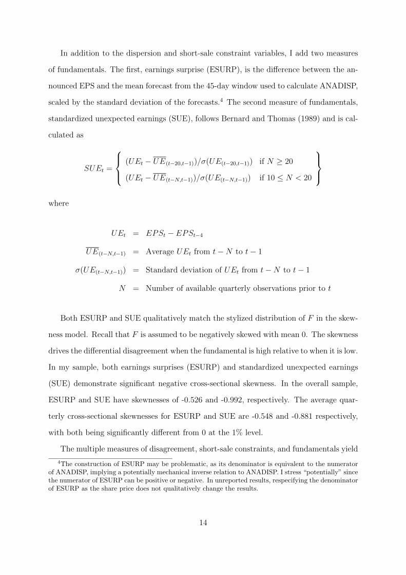
In addition to the dispersion and short-sale constraint variables, I add two measures

of fundamentals. The first, earnings surprise (ESURP), is the difference between the an-

nounced EPS and the mean forecast from the 45-day window used to calculate ANADISP,

scaled by the standard deviation of the forecasts.4 The second measure of fundamentals,

standardized unexpected earnings (SUE), follows Bernard and Thomas (1989) and is cal-

culated as

SUEt =

(UEt − UE(t−20,t−1))/σ(UE(t−20,t−1)) if N ≥ 20

(UEt − UE(t−N,t−1))/σ(UE(t−N,t−1)) if 10 ≤ N < 20

where

UEt = EPSt − EPSt−4

UE(t−N,t−1) = Average UEt from t−N to t− 1

σ(UE(t−N,t−1)) = Standard deviation of UEt from t−N to t− 1

N = Number of available quarterly observations prior to t

Both ESURP and SUE qualitatively match the stylized distribution of F in the skew-

ness model. Recall that F is assumed to be negatively skewed with mean 0. The skewness

drives the differential disagreement when the fundamental is high relative to when it is low.

In my sample, both earnings surprises (ESURP) and standardized unexpected earnings

(SUE) demonstrate significant negative cross-sectional skewness. In the overall sample,

ESURP and SUE have skewnesses of -0.526 and -0.992, respectively. The average quar-

terly cross-sectional skewnesses for ESURP and SUE are -0.548 and -0.881 respectively,

with both being significantly different from 0 at the 1% level.

The multiple measures of disagreement, short-sale constraints, and fundamentals yield

4The construction of ESURP may be problematic, as its denominator is equivalent to the numeratorof ANADISP, implying a potentially mechanical inverse relation to ANADISP. I stress “potentially” sincethe numerator of ESURP can be positive or negative. In unreported results, respecifying the denominatorof ESURP as the share price does not qualitatively change the results.

14

a large number of possible combinations (4× 2× 2) to analyze. In each test, the baseline

results use analyst dispersion, the indicative short-sale fee, and earnings surprises, under

the presupposition that these best represent the parameters in the theoretical models

discussed in Section 1. I then report results for all the remaining combinations. The

aggregate results prove to be largely consistent with each other. This robustness suggests

that the results are not driven by things specific to the disagreement measure, like analyst

career concerns (e.g., analysts may have incentives not to report their true beliefs), or by

sample selection (e.g., the intersection of firms with both analyst coverage and short-sale

fees reported in Markit).

For the monthly analysis, I follow DMS and use the I/B/E/S monthly summary file for

quarterly EPS forecasts, where ANADISP is again measured by the standard deviation

of analyst forecasts scaled by the mean forecast. Excess returns are calculated as the

monthly raw return less the CRSP value-weighted index over the same month.

3 Earnings Announcements

The key finding in DMS is that high analyst dispersion in month t predicts low returns at

t + 1, which they primarily explain this result via Miller (1977): High dispersion pushes

up the price at t, necessitating lower returns at t+1. BDJKT suggest a more rigorous test

of Miller involves the resolution of uncertainty such that the prior dispersion decreases.

They use earnings announcements as such a resolution, their rationale being that once

earnings are announced, there is less for agents to disagree upon.

In this section, I revisit BDJKT’s key tests on announcement returns and add parallel

tests for the realized fundamentals. The latter is to investigate the possibilities that

1) disagreement predicts fundamentals and 2) the return results are at least partially

driven by fundamentals. I then run multivariate regressions conditioning on the realized

fundamental to determine whether disagreement has any additional explanatory power

for future returns.

15

3.1 Single-Sorted Portfolios

BDJKT’s first tests involve sorting firms into quintiles by their pre-announcement dis-

agreement at the end of each quarter and averaging the subsequent earnings announce-

ment buy-and-hold abnormal return (BHAR) for each firm in the quintile. If the Miller

intuition is correct, high-disagreement firms should experience low BHARs.

Indeed, both BDJKT’s and my results confirm this. In Table 2, the first row of Panel A

lists average BHAR for firms sorted into quintiles based on their pre-announcement analyst

dispersion (ANADISP). The average BHAR across dispersion quintiles largely follows the

Miller-based prediction, increasing moderately from the first to second quintiles, then

decreasing monotonically thereafter. More relevantly, the difference in BHAR between

the lowest and highest quintiles is positive and statistically significant.

[Table 2 about here]

The second row lists the realized earnings surprise (ESURP) for firms in each quintile.

Remarkably, the pattern in earnings surprises is virtually identical to that in announce-

ment returns. ESURP is monotonically decreasing, with the difference between the lowest

and highest quintiles being positive and significant. This result lines up with the skewness

model’s H1 prediction, which states that the level of dispersion negatively predicts the

realized fundamental.

The result in the top two rows of Panel A in Table 2 represents the empirical starting

point for this paper. Abstracting from the legitimate concern about whether ESURP is

a reliable measure of the market-wide surprise in the earnings announcement, the par-

allel trends in BHAR and ESURP across disagreement open up the possibility that the

observed relationship between disagreement and future returns is driven at least in part

by a correlation between disagreement and the surprise in fundamentals. If this results

is generalizable beyond analyst dispersion and earnings suprise, it would not just be the

case that disagreement predicts returns. Disagreement would also predics the unpriced

bias in analysts’ forecasts. This is consistent with the skewness model’s prediction H1

16

in Table 1, but even if the skewness model is not correctly specified, the empirical result

is striking in its potential challenge to how we think of information flows and prices in

ostensibly efficient markets.

Having said that, ESURP may not be an appropriate proxy for the true (market)

surprise in fundamentals. A voluminous literature has analyzed the incentives of analysts

to report truthfully or accurately. For example, analysts have empirically been found to

be systematically optimistic, as in DeBondt and Thaler (1990) and Dreman and Berry

(1995). Trueman (1994) and Welch (2000) document that analysts tend to herd in their

recommendations. Theoretical models like Scharfstein and Stein (1990) and Lim (2001)

suggest that career concerns may shape analysts forecasts, and empirical papers like

Michaely and Womack (1999), Dechow, Hutton, and Sloan (1998), and Hong and Kubik

(2003) provide supportive evidence. Given these concerns, using a measure (ESURP)

based on what may be biased forecasts may not necessarily proxy for the true surprise in

earnings announcement. One may be similarly concerned that using analyst dispersion

as the measure of disagreement is confounded by analysts’ biases.

To address these concerns, I rerun the univariate tests involving quintile sorts using

the other 7 combinations of disagreement and fundamentals detailed in Section 2. The

results fill out the remainder of Table 2. Each pair of rows corresponds to a disagreement-

fundamental measures pair.

The second two rows of Panel A keep ANADISP as the disagreement measure but

use standardized unexpected earnings (SUE), an accounting measure, as the measure of

fundamentals. This change to the fundamentals alters the sample, as the set of observa-

tions with both ANADISP and ESURP is not identical to the set with both ANADISP

and SUE. By design, I do not restrict the samples to be identical for all disagreement

and fundamentals (and, later, short-sale constraint) combinations, so as to reduce the

possibility that the results are driven by sample selection issues. In this case, changing

the fundamentals to SUE does not qualitatively affect the results. SUE is monotonically

decreasing while BHAR is again nearly monotonically decreasing as one moves across

17

ANADISP quintiles. The positive and significant difference in BHAR across the lowest

and highest quintiles is matched by a positive and significant difference in SUE across the

two quintiles.

Using analyst forecasts to measure disagreement is potentially problematic if ana-

lysts have incentives to not report truthful forecasts. To attenuate this concern, I follow

BDJKT’s alternate measures of disagreement.

The prior stock return volatility (RETVOL) is a market-based measure of disagree-

ment and therefore less subject to the distortions that potentially affect analyst forecasts.

In Panel B, while the mean BHARs are not monotonically decreasing across RETVOL

quintiles, the Low - High estimates are positive and significant. The mean fundamentals

are monotonically decreasing, and the Low - High estimates match the BHAR results in

sign and significance.

Share turnover (TURN), defined as the percentage of shares traded daily, is another

market-based measure of disagreement. The results in the first two rows of Panel C are are

decidedly inconsistent with the skewness model. While the Low - High BHAR is positive

and significant, the corresponding differential ESURP is negative and significant. Looking

at the individual quintile averages, this result is even more puzzling. BHAR is roughly

flat across the first four TURN quintiles, then drops in the top quintile. Conversely,

ESURP is increasing as one moves across TURN quintiles. In and of itself, that ESURP

is increasing with TURN might be reconciled with a story about turnover increasing

when good news is to be revealed in fundamentals. But the corresponding low BHAR

suggests that the pre-announcement price was somehow too high relative to the realized

(good) fundamental. This outcome is not easily explained by a skewness-, overpricing-,

or risk-based model. When using SUE as the measure of fundamentals, I again observe

that fundamentals are declining with disagreement and that the differences in Low - High

BHAR and Low - High fundamentals line up with the baseline results.

Finally, income volatility (INCVOL) is used as an accounting-based measure of dis-

agreement. As reported in Panel D, the INCVOL results are mixed. In the ESURP

18

and the SUE samples, neither the average BHAR nor average fundamental is monotoni-

cally declining across INCVOL quintiles. In the first two rows, both the average BHAR

and ESURP are inverted-U shaped, with the Low - High mean BHAR and ESURP es-

timates positive and significant. Using SUE as measure of fundamentals, the positive

and significant Low - High difference in BHAR is paired with a corresponding negative

and significant difference in SUE. A confounding factor here is that INCVOL and SUE

are mechanically inversely related. The numerator of INCVOL is the prior volatility of

seasonally-adjusted operating income, while the denominator of SUE is the prior volatility

of seasonally-adjusted earnings. The average SUE in the sample is negative, so if the SUE

denominator is mechanically high for the high INCVOL group, the measured SUE will

be pushed toward 0 (and potentially above the SUE of the low INCVOL group). Should

this be the case, the INCVOL/SUE test is improperly specified.

Overall, the whole of Table 2 is largely directly supportive of the skewness model’s H1

prediction and inferentially supportive of its H2 prediction. 6 of the 8 (or 7, depending

on the validity of the INCVOL/SUE combination) tests are consistent with the skewness

model’s H1 prediction that high disagreement predicts low fundamentals. Moreover, in

these 6 tests, the positive and significant difference in Low - High BHAR is matched by

an equivalent result for the fundamental, supportive of the H2 prediction.

3.2 Double-Sorted Portfolios

The next set of tests in BDJKT double-sort firms into nine groups. Each quarter, firms are

assigned to Low (bottom 30%), Medium (middle 40%), and High (top 30%) groups based

on their ranked short-sale constraints. Within each of these groups, firms are sorted into

Low, Medium, and High groups based on their ranked disagreement. For a given short-sale

constraint group, if the Miller intuition is correct we should observe announcement returns

to be decreasing as disagreement increases. In the skewness model, there are no short-sale

restrictions, so there is limited inference to be made about returns or fundamentals across

varying levels of short-sale constraints. Holding fixed the level of short-sale constraints,

19

the intuition of the skewness model still applies.

Panel A of Table 3 lists the average earnings announcement BHAR for each of the nine

portfolios. The results are consistent with the equivalent tables in BDJKT, in that 1)

within a given short-sale constraint (the indicative fee in the present case versus institu-

tional ownership in BDJKT) group, the average BHAR is decreasing in pre-announcement

analyst dispersion and 2) within each analyst dispersion group, the average BHAR is de-

creasing in the level of the short-sale constraint.

[Table 3 about here]

Further examination of Panel A provides evidence both for and against Miller’s (1977)

hypothesis. On the one hand, conditioning on the short-sale constraint, higher disagree-

ment is associated with lower announcement returns, and conditioning on disagreement,

more binding short-sale constraints are associated with lower returns. These results align

with the Miller story. On the other hand, the positive and significant difference in an-

nouncement returns between the Low and High disagreement groups for the Low fee group

– the group that should be easily shorted – suggests that limits to arbitrage may not be

driving the return result.

In Panel B of Table 3, I calculate the average earnings surprise ESURP for each group

and document a comparable pattern for ESURP as for BHAR. Across a given short-sale

fee group, ESURP is decreasing with analyst dispersion. Within a given analyst dispersion

group, ESURP is decreasing with the short-sale fee. The results in Panel B are striking

in their ability to match the variation returns across the short-sale fee/analyst dispersion

groups.

In the context of the skewness model, absent significant differences in BHAR between

the Low and High short-sale constraint groups, conditioning on the disagreement group

to determine whether short-sale constraints are correlated with fundamentals is not infor-

mative. The skewness model has no prediction about what the difference in fundamentals

between Low and High short-sale constraint firms should be. Moreover, the order of the

20

sorting creates an empirical problem, one that can be conveyed with a representative

example. The analyst dispersion for the High FEE, Low ANADISP group may be very

different from the dispersion for the Low FEE, Low ANADISP group. Were it the case

that the differential BHAR within the Low disagreement group was not significant, the

positive and significant differential fundamentals would not shed light on the predictions

of the skewness model.

As before, the baseline analysis is subject to the possibility that the chosen measures

of disagreement, fundamentals, and short-sale constraints are inappropriate for testing

Miller’s (1977) and the skewness models. I rerun the tests across the remaining 15 com-

binations of disagreement, fundamentals, and short-sale constraints. For each of these

triples, I report the Low - High BHAR and the Low - High fundamental averages, both

within short-sale constraint groups and within disagreement groups.

Table 4 details the key results from applying the tests in Table 3 to every combination

of disagreement, fundamentals, and short-sale constraints. The first three columns report

the differences in average BHAR and average fundamentals between the Low and High

disagreement (DA) group, conditional on the short-sale constraint (SSC) group. The sec-

ond three columns report the differences between the Low and High short-sale constraint

group, conditional on the disagreement group. The table is split into four panels, one for

each measure of disagreement. Each panel is then split into two sets based on the short-

sale constraint used: the indicative fee (FEE) or the percentage of shares outstanding

not held by institutional investors (RETAIL). Each of those sets is then further split by

the measure of fundamentals. For reference, the top two rows of Panel A correspond to

the Low - High test statistics from Table 3. Each pair of subsequent rows represents the

equivalent statistics from running the same test procedure but with different combinations

of the disagreement, fundamental, and short-sale constraint measures.

[Table 4 about here]

Before unpacking Table 4, I’ll list what it is we might hope to learn from it:

21

1. Replicate BDJKT’s results, not only for the multiple measures of disagreement

but also for the multiple measures of short-sale constraints. By “replicate”, I’m

specifically referring to the majority of positive and significant differences in aver-

age BHAR between the Low and High disagreement (short-sale constraint) groups

within a given short-sale constraint (disagreement) group.

2. Determine whether disagreement is correlated with fundamentals conditional on the

short-sale constraint. Though the skewness model makes no reference to short-sale

constraints, its predictions should hold if we fix the level of the constraint: increasing

disagreement should predict lower fundamentals.

(The reverse test – whether disagreement is correlated with the short-sale constraint

conditional on the disagreement group – is not relevant, for the reason detailed in

the earlier discussion of Table 3.)

3. The final and ultimate goal is to observe whether the results for Low - High earnings

announcement BHARs within short-sale constraint groups and within disagreement

groups are matched by similar results for Low - High realized fundamentals within

those same groups. Confirmation of such a pattern, as found in Table 3, would

be consistent with the skewness model, which predicts the announcement returns

observed in BDJKT are driven by fundamentals and not disagreement itself.

With these considerations in mind, I have shaded cells in Table 4 in which 1) within a

short-sale constraint group, the difference in either BHAR or the fundamental is negative

and significant; or 2) within a disagreement group, the differential fundamental is not

positive and significant when the corresponding difference in BHAR is. The purpose of

the shading is to identify the results which run strongly counter to either the skewness

model’s or Miller’s predictions.

Some general patterns are observed across the four disagreement measures. Within

SSC groups, the differential BHAR is generally positive and significant, supporting both

Miller’s and my story. The cases in which the differential BHAR is not significant may

22

still be consistent with Miller, in that they generally occur for the Low and Medium SSC

groups, which by definition should be less affected by limits to arbitrage. Within SSC

groups, the majority of differential fundamentals are positive and significant, consistent

with the skewness model’s H1 prediction. The cases in which they are not positive echo

the cases from Table 2 (TURN/ESURP and INCVOL/SUE).

Within disagreement groups – i.e., the last three columns of Table 4 – the overwhelming

majority of differential BHARs are positive and significant, and these results are matched

by positive and significant differential fundamentals. This suggests that the portion of the

observed BHAR attributed to the interaction of disagreement and short-sale constraints

in prior literature may be at least partially explained by the realized fundamentals.

Working through the different disagreement measures one at a time, Panel A lists

results when disagreement is measured by analyst dispersion. The results are strongly

supportive of the skewness model’s central prediction that disagreement proxies for fun-

damentals. While the BHAR results are consistent with the Miller interpretation, the

ESURP and SUE results suggest that the observed announcement return is driven at

least partially by the realized fundamental. In virtually every case where the differential

BHAR is positive and significant, the realized fundamental is as well.

In Panel B, return volatility measures disagreement. Within SSC groups, the results

for differential BHAR here are comparatively less supportive of either the Miller or the

skewness model than they were Panel A. Specifically, one case (SSC = FEE, fundamental

= ESURP) generates negative and significant differential BHARs, implying that high

disagreement resulted in higher announcement returns. The results for fundamentals

are nevertheless strongly supportive of the skewness model’s prediction regarding their

relationship with disagreement. The average Low - High fundamentals are positive and

significant within each SSC group.

The disagreement measure in Panel C is share turnover. Echoing the results from Table

2, the sign on the differential ESURP within SSC groups is negative in 5 of the 6 tests.

Within TURN groups, the patterns in differential BHAR (i.e., positive and significant)

23

are matched in the patterns in differential fundamentals.

Panel D lists results when the disagreement measure is income volatility. Again, the

results here echo those from Table 2. Specifically, within short-sale constraint groups, the

differential SUE is negative and significant, but again, the caveat regarding a potentially

mechanical inverse relationship between INCVOL and SUE applies here. The within-

SSC-group results based on ESURP are largely consistent with the skewness model, in

that in 5 of the 6 tests, the sign and significance of the differential BHARs is matched by

those of the differential ESURPs.

Overall, the within-SSC-group results from Table 4 largely confirm those from the

single sorts in Table 2, that the observed difference in BHAR between low and high

disagreement stocks is generally accompanied by a corresponding difference in the realized

fundamental. The within-DA-group results further suggest that the observed differential

BHARs are driven in part by differential realized fundamentals.

3.3 Multivariate Analysis

The results in Sections 3.1 and 3.2 provide direct support for the skewness model’s H1,

that disagreement predicts the realized fundamental, but only inferential support for the

skewness model’s H2, that conditional on the fundamental, disagreement does not predict

announcement returns. To test H2, I construct a variation of the earnings response models

used in the accounting literature5.

Each quarter t, I sort firm i into quintile q based on its realized fundamental. Then,

for each q, I run Fama-MacBeth regressions on the following model:

BHARit = αq + β1qDAit + β2qSSCit + β3qDAit × SSCit (4)

where BHARit is i’s earnings announcement BHAR at t; DAit is i’s pre-announcement

disagreement; SSCit is its pre-announcement level of the short-sale constraint; and DAit×5See, for example, Collins and Kothari (1989).

24

SSCit is the interaction of disagreement and the short-sale constraint. Casually observed,

Equation (4) appears to be an earnings response model without earnings. Rather, it’s an

earnings response model in which the earnings response coefficient times the average of

the measure of earnings is represented by the intercept αq for each q.

With regards to Miller’s and the skewness model’s respective H2’s, the predictions

for the coefficients in Equation (4) are clear. According to the Miller model, having

conditioned on the realized fundamental, the coefficient on DA× SSC – and, depending

on one’s interpretation of Miller, on DA – should be negative. By contrast, according to

the skewness model, having conditioned on the realized fundamental F , the coefficients

on DA and DA×SSC should be zero. Failing that, a supportive if not confirming result

would be for the coefficients to be negative for the lower realized fundamental quintiles

and positive for the higher realized fundamental quintiles. This result would be obtained

if the mean of λ were negatively correlated with the magnitude of F . That is, if high

absolute F was tied to low µλ, then the pre-announcement price would be relatively closer

to the pre-signal price, implying the announcement return would be greater in magnitude

than it would be if µλ were uncorrelated with disagreement.

Table 5 presents results from the baseline ANADISP/FEE/ESURP combination. Each

column represents observations in which a firm was in the qth quintile in ESURP for a

given quarter. ANADISP and FEE are the winsorized raw (unranked) measures of analyst

dispersion and indicative fees.

[Table 5 about here]

Looking at the results, the constant terms line up as one would expect, increasing

monotonically with the earnings surprise quintile. More importantly, the results for

ANADISP and ANADISP×FEE are largely consistent with my H2 and entirely inconsis-

tent with the corresponding Miller prediction. Conditioning on the realized fundamental,

neither analyst dispersion nor its interaction with the short-sale fee has a negative and

significant statistical correlation with the announcement return. Even if the mechanism in

25

the skewness model is not correct, what is clear from Table 5 is that the Miller mechanism

is not driving the majority of the cross-sectional variation in BHAR. In two of the ten

cases, the coefficient is positive and significant, suggesting that higher dispersion leads

to higher returns even after conditioning for the realized fundamental. Moreover, if one

were to relax the assumption applied to Miller that disagreement is not correlated with

the fundamental and argue that limits to arbitrage drive the pre-announcement price up,

we should observe in the coefficients for ANADISP, FEE and ANADISP×FEE all being

negative for the lower quintiles, but this is not borne out in the results.

Table 6 tabulates results from estimating Equation (4) for each quintile based on the

remaining 15 combinations of disagreement, short-sale constraints, and fundamentals. To

keep the table size manageable, I report only the coefficients on the disagreement measure

(DA) and its interaction with the short-sale constraint measure (DA×SSC). With regard

to the omitted coefficients:

1. As one might expect, the constant term is increasing monotonically with the fun-

damentals quintile in nearly every specification. In the instances where this is not

the case, the constant term is not significant.

2. For no combination is there a pattern in the short-sale constraint coefficients that

is consistent with a Miller story. There are sporadic instances of one or (rarely)

two SSC coefficients being negative and significant, but there are a similar number

of instances where the coefficient is positive and significant. The sum of the SSC

results weigh strongly against a Miller interpretation.

[Table 6 about here]

As before, the table has four panels, one for each disagreement measure. Before

discussing the individual results, I’ll summarize the cumulative takeaway: For no combi-

nation of disagreement, short-sale constraints, and fundamentals are the coefficients on

DA×SSC uniformly negative across all quintiles. The Miller story implies that the co-

efficient on DA×SSC should be negative and significant, yet, as seen by the five shaded

26

cells in Table 6, this is true in only a small minority of the test cases. There are sporadic

instances in which either the coefficient on DA or DA×SSC is negative and significant,

but the vast majority of the estimated coefficients are either insignificant or occasionally

positive and significant.

Working through the individual results, Panel A lists the results using ANADISP

as the measure of disagreement. The results here overwhelmingly support the skewness

model over Miller’s. There is only one instance in which the coefficient on DA is negative

and significant (Quintile 1, RETAIL/SUE) and no instance in which DA×SSC is negative

and significant. The results strongly support the hypothesis that disagreement drives

returns only through their correlation with future realized fundamentals.

In Panel B, I report results using RETVOL to measure disagreement. As opposed

to the ANADISP-based estimates, the coefficients on RETVOL are significant in a large

number of cases, though the relative ordering of these coefficients across quintiles is poten-

tially more suggestive of the skewness model than Miller’s. Take, for instance, the results

for the FEE/ESURP combination in the first two rows of the panel. The coefficients on

DA are negative for the Low fundamental quintile and then monotonically increasing as

we move across quintiles. This is consistent with the scenario I detailed earlier, in which

the magnitude of |F | is correlated with the mean of λ. But this interpretation requires

a fairly generous reading of the model. The most accurate reading of the monotonically

increasing point estimates is that they support neither the Miller nor skewness model.

The results when TURN measures disagreement are reported in Panel C. While there

are five cases in which the coefficient on DA is negative and significant and four cases in

which the coefficient on DA×SSC is negative and significant, overall the TURN results

strongly support the skewness model over Miller’s.

Finally, Panel D lists results when INCVOL is the measure of disagreement. Again,

despite the occasional negative and significant coefficient on either DA or DA×SSC (as

well as a positive and significant coefficient, twice), the INCVOL results strongly support

the skewness model over Miller’s.

27

The lack of negative and significant coefficient estimates for DA×SSC works strongly

against a Miller interpretation and for the skewness model’s predictions. Given that I

control for SSC and its interaction with DA, the instances of negative and significant

coefficients for DA are not necessarily supportive of Miller. That they are predominantly

confined to the lower fundamental quintiles and that they are in some cases matched by

positive and significant coefficients for the higher fundamental quintiles can be reconciled

in the skewness model if one allows for the mean of the weights (µλ) to be negatively

correlated with the magnitude of the fundamental (|F |).

Taken together, the single-sorted, double-sorted, and multivariate results in this sec-

tion provide support of the skewness model’s two predictions (H1 and H2) regarding

fundamentals. In the majority of test specifications, disagreement is correlated with fu-

ture fundamentals, and the realization of the fundamental and not disagreement itself

drives the realized earnings announcement return.

4 Monthly Returns

In this section, I revisit the monthly dispersion-return relationship documented in DMS.

The innovation is to frame the analysis in terms of changes in dispersion, truer in some

sense to the original Miller proposition. The section is intended to test the respective H3

through H5 predictions listed in Panel B of Table 1.

According to the skewness model, high disagreement at t should correspond to low

contemporaneous returns Rt (H4); high disagreement at t and t + 1 should correspond

to high t + 1 returns Rt+1 (H4A); and high disagreement at t and low disagreement

at t + 1 should correspond to low t + 1 returns (H4B). H5, H5A, and H5B are the

corresponding opposite predictions for low disagreement at t. The predictions can be

summarized compactly: Returns at t is negatively correlated with the contemporaneous

disagreement. This contrasts with the Miller predictions, which are no prediction for Rt

conditional on Dt; zero (excess) return when Dt and Dt+1 are both high or both low; and

28

high (low) Rt+1 when Dt is low (high) and Dt+1 is high (low).

In my first tests, each month I sort firms into quintiles based on their monthly analyst

dispersion, as measured using the monthly summary measures from I/B/E/S. I create

25 unequal portfolios based on firms’ t and t + 1 dispersion quintiles, then report the

mean t+ 1 monthly portfolio excess return, measured as the raw return minus the CRSP

value-weighted index for the month. Results are presented in Table 7. To read the table,

(e.g.) the cell corresponding to ANADISPt = 1 and ANADISPt+1 = 3 reports the average

next-month excess return for firms which were in the lowest (1) analyst dispersion quintile

in the current month and in the middle (3) quintile in the next month.

[Table 7 about here]

DMS’s key observation is the final column of Table 7, which shows next-month re-

turns clearly declining with dispersion. What’s unclear in their analysis is what the null

hypothesis should be regarding the time-series of dispersion. Should dispersion be mean

reverting (median reverting, more precisely), in which case firms on average move in and

out of the middle quintile? If so, the Miller logic implies that high-dispersion stocks should

experience low future returns, and low-dispersion stocks should experience high future re-

turns, assuming movements in short-sales constraints aren’t correlated with dispersion.

This would seem to fit the results in the final column.

Alternatively, should dispersion be serially correlated? In this case, the Miller model

would predict (as in H4 and H5) average returns for firms whose dispersion didn’t change;

high returns for firms whose dispersion increased; and low returns for firms who dispersion

decreased. The two-way results in Table 7 do not support these predictions and instead

imply that the next-month returns are driven by serial correlation in disagreement, con-

sistent with the T > 2 extension of the skewness model. Fixing the month t dispersion

(i.e., moving across a given row), the average t+ 1 excess returns are decreasing with the

t + 1 dispersion, exactly what my extended model predicts and exactly the opposite of

what the Miller model predicts. What the final column – and what DMS – is picking up

29

is predominantly the diagonal of the matrix. Dispersion at t is correlated with dispersion

at t + 1, and if dispersion at t + 1 drives the contemporaneous return, it will appear as

though dispersion at t predicts future returns.

A potential concern with this analysis is that one third of the observations overlap

with earnings announcements, potentially confounding the results. In unreported results,

I rerun the tests, first including only firm-months without a quarterly earnings announce-

ment and second including only firm-months with a quarterly earnings announcement.

The results are not qualitatively different in either subsample.

My next tests build on the underlying dynamics revealed in Table 7. For each firm-

month, I calculate the change in dispersion quintile from the prior to the current month.

I then calculate the average monthly excess return for all stocks with a given change in

quintiles. Table 8 displays the average excess return based on the change in quintiles, as

well as the number of observations with that change. Two results can be seen:

1. Dispersion is not mean/median-reverting but rather serially correlated. The major-

ity of observations are clustered at 0: no change in the ranked dispersion from one

month to the next. 90% of the observations are clustered between -1 and +1.

2. Excess returns are negatively related to changes in dispersion, consistent with the

skewness model and inconsistent with Miller’s.

[Table 8 about here]

To identify the extent to which returns are driven by correlation with contemporaneous

dispersion as opposed to correlation with the change in dispersion, I run two sets of Fama-

MacBeth regressions where the t + 1 excess return is the dependent variable. Unlike

earlier tests, here I use the actual dispersion measure, not the quintile rank. In the

first specification, the explanatory variable is ∆ANADISP, the (1%, 99%) winsorized

raw change in analyst dispersion from month t to t + 1. Column 1 of Table 9 reports

a negative and significant coefficient on the change in analyst dispersion, inconsistent

30

with Miller and consistent with the skewness model. In the second specification, I add

the explanatory variable ANADISPt+1, the winsorized analyst dispersion at t + 1. In

Column 2, again consistent with the skewness model’s predictions and inconsistent with

their Miller counterparts, I find the coefficient on ANADISPt+1 is negative and significant,

with the coefficient on ∆ANADISP no longer being statistically significant.

[Table 9 about here]

In sum, the results indicate that 1) returns are negatively correlated with the contem-

poraneous level of disagreement and 2) the predictive relationship between disagreement

and future returns is driven by serial correlation in disagreement. The Miller mechanism

finds little support in the results, as does a risk-based hypothesis, which predicts high

returns when dispersion is high for consecutive periods. That returns are not driven by

prior disagreement but rather current disagreement is consistent with my extended model

in which changes in disagreement correspond to new information about the fundamental.

5 Analyzing Disagreement

Excluding income volatility INCVOL, the remaining three disagreement measures used in

Section 3 reflect the actions of market participants – analysts and investors – over 45-day

windows. In this section, I calculate characteristics of these three disagreement measures

over their estimation windows to shed additional light on the dynamics underlying the

preceding results. In Table 10, I present averages for the calculated characteristics, sorted

by the dispersion quintile. The purpose here is exploratory, so I do not run formal tests

other than simple difference-in-means t-tests. I do not run t-tests on the individual aver-

ages, since for many of the variables it is not clear what the appropriate null-hypothesis

values should be.

31

5.1 Analyst Dispersion

For the sample underlying each analyst dispersion (ANADISP) observation, I calculate

NUMANALYSTS, the number of unique analysts issuing forecasts. Hong, Lim, and Stein

(2000) argue that the number of analysts covering a firm proxies for the speed at which

negative information about that firm diffuses. The first row of Panel A in Table 10

indicates that high analyst dispersion is correlated with lower analysts covering the firm,

with the difference in average analyst coverage between the lowest and highest quintiles

positive and statistically significant, suggesting the possibility that part of the mechanism

driving higher disagreement is lower analyst coverage.

[Table 10 about here]

LOWLATE is calculated as the proportion of the forecasts below the median (“low”)

in the estimation window which were submitted after the median announcement date

(“late”). LOWLATE conveys whether the lower forecasts in the estimation window tended

to occur early or late relative to higher forecasts. LOWLATE being positively correlated

with analyst dispersion is consistent with the theory advanced in Hong, Lim, and Stein

(2000), where good and bad information diffuse asymmetrically, if analysts are heteroge-

neous in their speed of adopting a common signal. This is exactly what is observed in the

second row of Panel A: LOWLATE is increasing with analyst dispersion.

SKEW(FC) is the skewness of the analysts’ (final) forecasts. The motivating question

is whether high disagreement tends to be caused by asymmetric outliers. The third row

of Panel A indicates that the skewness of forecasts is on average increasing with analyst

dispersion. In particular, high analyst dispersion stocks have positively skewed forecasts.

The skewness neither supports nor falsifies the skewness model but rather gives some

indication of what the distribution of λn might be.

Finally, I calculate BELOWMEDIAN as the proportion of forecasts which were below

the trailing five-forecast6 median at the time they were announced. BELOWMEDIAN

6The trailing five-forecast window includes forecasts which were not used to calculate ANADISP.

32

indicates whether forecasts were predominantly negative relative to those issued imme-

diately prior. In the fourth row of Panel A, I document average BELOWMEDIAN is

increasing with analyst dispersion, suggesting that high dispersion is on average driven

by relatively negative forecasts.

5.2 Return Volatility

For each 45-day return volatility (RETVOL) estimation window, I calculate CUME-

EXRET as the cumulative buy-and-hold return of the stock less the corresponding buy-

and-hold return on the CRSP Value-Weighted index. If the skewness model is correct and

returns trend toward the yet unrealized fundamental, CUMEEXRET should be lower for

high RETVOL observations. The first row of Panel B in Table 10 indicates the oppo-

site: The highest RETVOL observations have significantly higher CUMEEXRET than

the lowest RETVOL observations.

The second row of Panel B documents NEGEXRET, the proportion of the 45 daily

excess returns which were negative. A higher proportion of negative daily returns for

high disagreement stocks is consistent with my extended model, as information diffuses

according to the mean weight λ.

SKEW(EXRET), in the third row of Panel B, is the skewness of the daily excess

returns. Similar to NEGEXRET, the skewness indicates whether the return volatility

was driven by predominantly low returns, predominantly high returns, or neither. Similar

to SKEW(FC), SKEW(EXRET) is larger for high RETVOL observations relative to low

RETVOL observations. In sum, CUMEEXRET, NEGEXRET, and SKEW(EXRET) all

indicate that high RETVOL observations tend to be driven by predominantly negative

daily excess returns with infrequent, relatively high positive daily excess returns.

5.3 Turnover

I calculate SD(DTURN) as the standard deviation of the 45 daily turnover observations.

In the first row of Panel C, I document that high TURN observations are characterized

33

by significantly higher daily turnover volatility.

SKEW(DTURN), in the second row of Panel C, is the skewness of daily turnover over

the 45-day estimation window. Unlike SKEW(FC) and SKEW(EXRET), SKEW(DTURN)

is lower for the high disagreement (TURN) quintile relative to the low disagreement quin-

tile, though the average is similar across all five quintiles, which limits the inference one

can draw.

EARLY-LATE is calculated as the difference in the average daily turnover over the

first 22 days (“early”) minus the average over the second 23 days (“late”). The average

EARLY-LATE is either flat or increasing over the first four TURN quintiles, with a sharp

decrease at the fifth quintile. This suggests that when TURN is high, it is on average due

to late increases in turnover.

6 Conclusion

In this paper, I find strong evidence that disagreement predicts the unpriced component

of the surprise in fundamentals. Across both univariate disagreement sorts and two-way

short-sale constraint/disagreement sorts, the pattern in earnings announcement returns

is matched by a corresponding pattern in fundamentals. Conditioning on the ex-post

fundamental, I find little evidence that disagreement has any predictive ability on the

earnings announcement returns. These results hold across a number of different measures

of disagreement, short-sale constraints, and fundamentals. Revisiting the relationship be-

tween monthly analyst dispersion and future returns documented in DMS, I find that the

previously-observed negative correlation is driven virtually exclusively by serial correlation

in dispersion and negative correlation between returns and contemporaneous dispersion.

To frame the results, I present a simple model linking skewness in fundamentals to

disagreement and returns. I take respective predictions of the skewness model, a Miller

(1977) based model, and a risk-based model to the data. Cumulatively, the results are

consistent neither with a Miller story, in which disagreement drives up the current price

34

which then falls as disagreement dissipates, nor with a risk-based model in which disagree-

ment proxies for risk and drives the contemporaneous price down and expected returns

up. By and large, the results support the predictions of the skewness model. If the

mechanism in the skewness model is in fact correct, or more generally if the results are

driven by some form of cognitive bias, the results raise the unanswered question of how

such a pattern in returns can exist without arbitrageurs bidding it down. If the model is

incorrect and the results are driven by rational agents trading optimally, the challenge is

to identify what such a mechanism might look like.

35

Table 1: Comparison of model predictions. Dt is disagreement at date t, Ft+1 is thefundamental realized at t+ 1, and Rt is the return at t. The expectation operator refersto the ex-post expected average, conditional on the (ex-post) observable. Given the use ofranked variables in the empirical tests, the notation “<0” and “>0” may be interpretedas “relatively low” and “relatively high”, respectively.

Panel A: Earnings AnnouncementsPrediction

Conditional on: Skewness Model Miller

H1 High Dt E[Ft+1] < 0 E[Ft+1] = 0H2 Ft+1 ρ(Dt, Rt+1) = 0 ρ(Dt, Rt+1) < 0

Panel B: Monthly ReturnsPrediction

Conditional on: Skewness Model Miller

H3 ρ(Dt, Dt+1) > 0 No prediction

H4 High Dt E[Rt] < 0 No predictionH4A High Dt → High Dt+1 E[Rt+1] < 0 E[Rt+1] = 0H4B Low Dt → High Dt+1 E[Rt+1] < 0 E[Rt+1] > 0

H5 Low Dt E[Rt] > 0 No predictionH5A Low Dt → Low Dt+1 E[Rt+1] > 0 E[Rt+1] = 0H5B High Dt → Low Dt+1 E[Rt+1] > 0 E[Rt+1] < 0

36

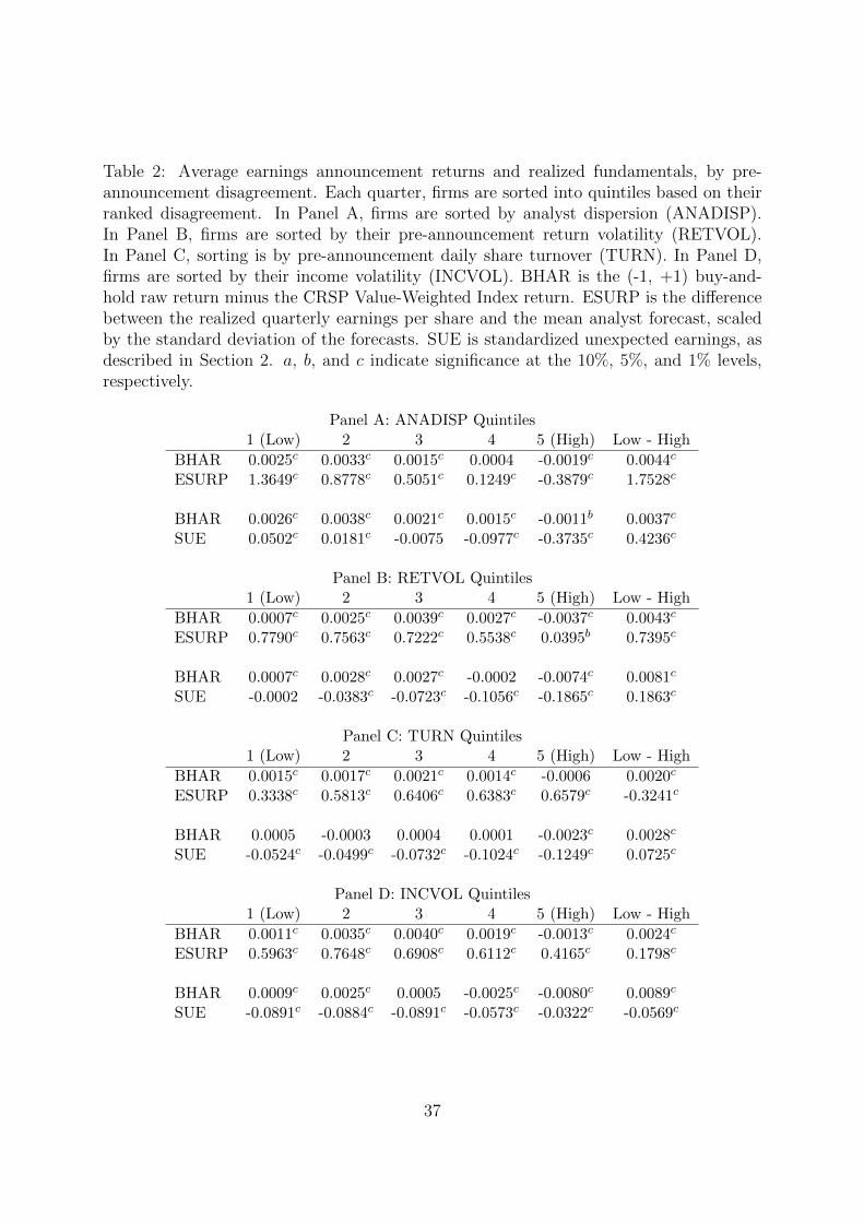
Table 2: Average earnings announcement returns and realized fundamentals, by pre-announcement disagreement. Each quarter, firms are sorted into quintiles based on theirranked disagreement. In Panel A, firms are sorted by analyst dispersion (ANADISP).In Panel B, firms are sorted by their pre-announcement return volatility (RETVOL).In Panel C, sorting is by pre-announcement daily share turnover (TURN). In Panel D,firms are sorted by their income volatility (INCVOL). BHAR is the (-1, +1) buy-and-hold raw return minus the CRSP Value-Weighted Index return. ESURP is the differencebetween the realized quarterly earnings per share and the mean analyst forecast, scaledby the standard deviation of the forecasts. SUE is standardized unexpected earnings, asdescribed in Section 2. a, b, and c indicate significance at the 10%, 5%, and 1% levels,respectively.

Panel A: ANADISP Quintiles1 (Low) 2 3 4 5 (High) Low - High

BHAR 0.0025c 0.0033c 0.0015c 0.0004 -0.0019c 0.0044c

ESURP 1.3649c 0.8778c 0.5051c 0.1249c -0.3879c 1.7528c

BHAR 0.0026c 0.0038c 0.0021c 0.0015c -0.0011b 0.0037c

SUE 0.0502c 0.0181c -0.0075 -0.0977c -0.3735c 0.4236c

Panel B: RETVOL Quintiles1 (Low) 2 3 4 5 (High) Low - High

BHAR 0.0007c 0.0025c 0.0039c 0.0027c -0.0037c 0.0043c

ESURP 0.7790c 0.7563c 0.7222c 0.5538c 0.0395b 0.7395c

BHAR 0.0007c 0.0028c 0.0027c -0.0002 -0.0074c 0.0081c

SUE -0.0002 -0.0383c -0.0723c -0.1056c -0.1865c 0.1863c

Panel C: TURN Quintiles1 (Low) 2 3 4 5 (High) Low - High

BHAR 0.0015c 0.0017c 0.0021c 0.0014c -0.0006 0.0020c

ESURP 0.3338c 0.5813c 0.6406c 0.6383c 0.6579c -0.3241c

BHAR 0.0005 -0.0003 0.0004 0.0001 -0.0023c 0.0028c

SUE -0.0524c -0.0499c -0.0732c -0.1024c -0.1249c 0.0725c

Panel D: INCVOL Quintiles1 (Low) 2 3 4 5 (High) Low - High

BHAR 0.0011c 0.0035c 0.0040c 0.0019c -0.0013c 0.0024c

ESURP 0.5963c 0.7648c 0.6908c 0.6112c 0.4165c 0.1798c

BHAR 0.0009c 0.0025c 0.0005 -0.0025c -0.0080c 0.0089c

SUE -0.0891c -0.0884c -0.0891c -0.0573c -0.0322c -0.0569c

37

Table 3: Double-sorted portfolios based on short-sale indicative fees (FEE) and analystdispersion (ANADISP). Following BDJKT, each quarter firms are sorted into low (bottom30%), medium (middle 40%), and high (top 30%) groups based on their ranked FEE.Within each FEE group, firms are sorted into low, medium, and high groups based ontheir ranked ANADISP. Panel A reports average earnings announcement buy-and-holdabnormal returns (BHAR), and Panel B reports average earnings surprises (ESURP). a,b, and c indicate significance at the 10%, 5%, and 1% levels, respectively.

Panel A: Earnings Announcement Abnormal Return (BHAR)ANADISP Group

Low Medium High Low - HighFee GroupLow 0.0036c 0.0030c 0.0016c 0.0020c

Medium 0.0041c 0.0021b -0.0011 0.0052c

High -0.0014 -0.0044c -0.0054c 0.0040b

Low - High 0.0050c 0.0074c 0.0070c

Panel B: Earnings Surprise (ESURP)ANADISP Group

Low Medium High Low - HighFee GroupLow 1.9137c 1.0362c 0.3119c 1.6018c

Medium 1.6646c 0.7995c 0.0671 1.5975c

High 1.0587c 0.1230c -0.3108c 1.3696c

Low - High 0.8550c 0.9132c 0.6228c

38

Table 4: Summary of tests for portfolios double-sorted on short-sale constraints (SSC)and disagreement (DA). Each quarter, firms are sorted into three groups (Low, Medium,and High) based on their ranked short-sale constraints. Within each short-sale constraintgroup, firms are then sorted into three groups based on their ranked disagreement. Thefirst (last) three columns report the difference in average BHAR and average fundamentalsbetween the Low and High DA (SSC) groups within a given SSC (DA) group. a, b, andc indicate significance at the 10%, 5%, and 1% levels, respectively.

SSC Group DA GroupShort-Sale BHAR/ Low Med. High Low Med. HighConstraint Fund’l Diff: Low - High DA Group Diff: Low - High SSC Group

Panel A: Disagreement (DA) Measure = ANADISP

FEEBHAR 0.0020c 0.0052c 0.0040b 0.0050c 0.0074c 0.0070c

ESURP 1.6018c 1.5975c 1.3696c 0.8550c 0.9132c 0.6228c

FEEBHAR 0.0017b 0.0047c 0.0024 0.0052c 0.0066c 0.0059c

SUE 0.2318c 0.2457c 0.2459c 0.1040c 0.1276c 0.1181c

RETAILBHAR 0.0032c 0.0026c 0.0052c 0.0034c 0.0053c 0.0055c

ESURP 1.4897c 1.3726c 1.2954c 0.7899c 0.7630c 0.5956c

RETAILBHAR 0.0026c 0.0018b 0.0046c 0.0028c 0.0048c 0.0048c

SUE 0.2767c 0.3360c 0.3867c -0.0056 0.0139 0.1044c

Panel B: Disagreement (DA) Measure = RETVOL

FEEBHAR -0.0026c 0.0034b 0.0119c -0.0002 0.0059c 0.0143c

ESURP 0.4047c 0.4813c 0.6444c 0.7383c 0.7219c 0.9780c

FEEBHAR -0.0007 0.0078c 0.0197c -0.0003 0.0110c 0.0201c

SUE 0.0937c 0.0715c 0.1290c 0.1015c 0.1029c 0.1367c

RETAILBHAR 0.0000 0.0005 0.0076c 0.0021c 0.0028c 0.0098c

ESURP 0.3086c 0.5147c 0.6048c 0.6001c 0.6631c 0.8963c

RETAILBHAR -0.0004 0.0017b 0.0092c 0.0014c 0.0044c 0.0110c

SUE 0.1462c 0.1625c 0.1739c 0.0273b 0.0170 0.0551c

Panel C: Disagreement (DA) Measure = TURN

FEEBHAR -0.0004 0.0013 0.0106c 0.0011 0.0065c 0.0121c

ESURP -0.2261c -0.2819c -0.1304a 0.6397c 0.9765c 0.7353c

FEEBHAR -0.0009 -0.0020 0.0086c 0.0051c 0.0105c 0.0146c

SUE 0.0512c -0.0002 0.0900c 0.0957c 0.1084c 0.1346c

RETAILBHAR -0.0001 0.0006 0.0083c 0.0010 0.0040c 0.0093c

ESURP -0.1830c -0.0790b 0.0869b 0.5882c 0.7009c 0.8581c

RETAILBHAR -0.0010 0.0018c 0.0091c 0.0007 0.0054c 0.0108c

SUE 0.0625c 0.1093c 0.0638c 0.0449c 0.0102 0.0462c

Panel D: Disagreement (DA) Measure = INCVOL

FEEBHAR 0.0005 0.0040b 0.0099c 0.0007 0.0075c 0.0100c

ESURP 0.0672a -0.1449a 0.1913b 0.7693c 0.7548c 0.8934c

FEEBHAR 0.0018c 0.0057c 0.0142c 0.0050c 0.0121c 0.0174c

SUE -0.0444c -0.1963c -0.0912c 0.1183c 0.0843c 0.0715c

RETAILBHAR 0.0009 0.0020c 0.0032c 0.0032c 0.0043c 0.0056c

ESURP 0.0044 0.1635c 0.1961c 0.6839c 0.7348c 0.8756c

RETAILBHAR 0.0013b 0.0035c 0.0091c 0.0039c 0.0060c 0.0118c

SUE -0.0411c -0.0595c -0.0408c -0.0066 -0.0009 -0.0064

39

Table 5: Fama-Macbeth regressions of earnings announcement buy-and-hold abnormalreturns (BHAR), by earnings surprise (ESURP) quintiles. ANADISP and FEE are thewinsorized raw (unranked) pre-announcement analyst dispersion and indicative short-sale fee, respectively. a, b, and c indicate significance at the 10%, 5%, and 1% levels,respectively

ESURP Quintiles1 (Low) 2 3 4 5 (High)

ANADISP -0.0001 -0.0008 0.0033 0.0153c -0.0023(-0.03) (-0.44) (1.39) (3.71) (-0.32)

FEE -0.0652 -0.1823b -0.1512 -0.0127 -0.1727b

(-1.11) (-2.48) (-1.62) (-0.11) (-2.18)ANADISP x FEE 0.3938 0.3912b 0.1456 -0.5019 2.3056

(1.26) (2.22) (0.46) (-0.90) (1.64)Constant -0.0389c -0.0128c 0.0027c 0.0177c 0.0356c

(-27.97) (-14.41) (3.43) (17.40) (30.11)Observations 21395 21389 21586 21591 21593R2 0.017 0.014 0.018 0.027 0.017

40

Table 6: Fama-Macbeth regressions of earnings announcement buy-and-hold abnormalreturns (BHAR), by realized fundamental quintiles. Coefficient estimates from regress-ing BHAR on disagreement (DA) and its interaction with the short-sale constraint(DA×SSC). Shaded cells indicate coefficients consistent with the Miller (1997) overpricingtheory. a, b, and c indicate significance at the 10%, 5%, and 1% levels, respectively.

SSC/FUND Independent Fundamental (FUND) QuintileMeasure Variable 1 (Low) 2 3 4 5 (High)

Panel A: Disagreement Measure (DA) = ANADISP

FEE/ESURPDA -0.0001 -0.0008 0.0033 0.0153c -0.0023

DA x SSC 0.3938 0.3912b 0.1456 -0.5019 2.3056

FEE/SUEDA -0.0026 -0.0022 -0.0016 0.0096 0.0079

DA x SSC 0.2622 0.2312 0.5606 -1.9394 -0.3878

RETAIL/ESURPDA 0.0022 0.0044 0.0054a 0.0044 0.0219a

DA x SSC -0.0021 -0.0076 -0.006 0.0079 -0.0117

RETAIL/SUEDA -0.0077b -0.0091 -0.0007 0.0048 -0.007

DA x SSC 0.0114a 0.0162 0.0018 -0.0036 0.0223a

Panel B: Disagreement Measure (DA) = RETVOL

FEE/ESURPDA -0.2944c -0.2051c 0.0476 0.3915c 0.4896c

DA x SSC 3.2741 -3.0959 -14.2832a -9.0676 2.6653

FEE/SUEDA -0.3458c -0.3701c -0.1685a -0.0262 -0.0105

DA x SSC 2.0393 3.9544 -2.689 -5.1619 -3.1458

RETAIL/ESURPDA -0.2608 -0.0644 0.0368 0.3733c 0.5508c

DA x SSC -0.19 -0.2895 -0.1788 -0.4354b -0.3214

RETAIL/SUEDA -0.3379b -0.0892 0.0741 0.0436 0.4260c

DA x SSC -0.0078 -0.2053 -0.256 -0.0109 -0.4249b

Panel C: Disagreement Measure (DA) = TURN

FEE/ESURPDA -0.0005b -0.0003c -0.0002 0.0002 0.0001

DA x SSC -0.0068 -0.0251a -0.0335 -0.0238 0.0016

FEE/SUEDA -0.0001 0.0000 0.0001 -0.0003a -0.0002a

DA x SSC 0.0068 -0.0100 -0.0078 0.0257 -0.0127

RETAIL/ESURPDA -0.0004 -0.0006 0.0001 -0.0006 0.0007a

DA x SSC -0.0005 0.0001 -0.0009 0.0007 -0.0003

RETAIL/SUEDA -0.0011b 0.0004 0.0007 0.0001 0.0011c

DA x SSC 0.0011a -0.0009a -0.0015a -0.0004 -0.0024c

Panel D: Disagreement Measure (DA) = INCVOL

FEE/ESURPDA -0.0841a -0.0782b -0.1039 0.0187 0.1151b

DA x SSC 6.1860b 5.1881 8.8721 -7.7627 -17.2149

FEE/SUEDA -0.0868b -0.0925b -0.0288 -0.0243 -0.0755

DA x SSC 0.4104 3.3506a 1.8545 -1.2916 3.5393

RETAIL/ESURPDA -0.0978 -0.2604b 0.0081 -0.0212 0.1676a

DA x SSC 0.0126 0.3266a -0.0138 0.1409 -0.1886

RETAIL/SUEDA -0.0645 -0.0783 0.0164 0.0803 0.2048b

DA x SSC -0.0394 0.0301 -0.0654 -0.1 -0.2600b

41

Table 7: Mean t+ 1 Excess Returns for (ANADISPt, ANADISPt+1) Quintile Pairs. Eachmonth, firms are sorted into quintiles by their analyst dispersion. Firms are then allocatedto unequal portfolios based on their t and t+1 dispersion quintiles. The mean t+1 excessreturn is reported for each (t, t + 1) quintile pair. a, b, and c indicate significance at the10%, 5%, and 1% values, respectively.

ANADISPt ANADISPt+1 QuintileQuintile 1 (Low) 2 3 4 5 (High) All1 (Low) 0.0083c 0.0034c 0.0046c 0.0011 -0.0042a 0.0067c

2 0.0052c 0.0015c -0.0019c -0.0073c -0.0231c 0.0004a

3 0.0054c 0.0027c 0.0017c -0.0026c -0.0230c 0.00024 0.0063c 0.0054c 0.0032c 0.0016c -0.0108c 0.0003

5 (High) 0.0072c 0.0005 0.0010 0.0050c -0.0030c -0.0018c

All 0.0080c 0.0021c 0.0017c 0.0010c -0.0050c

42

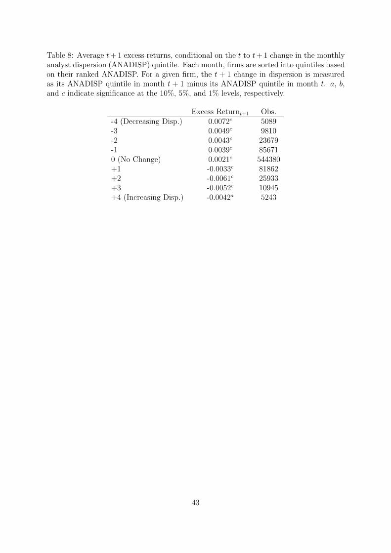
Table 8: Average t+ 1 excess returns, conditional on the t to t+ 1 change in the monthlyanalyst dispersion (ANADISP) quintile. Each month, firms are sorted into quintiles basedon their ranked ANADISP. For a given firm, the t + 1 change in dispersion is measuredas its ANADISP quintile in month t + 1 minus its ANADISP quintile in month t. a, b,and c indicate significance at the 10%, 5%, and 1% levels, respectively.

Excess Returnt+1 Obs.-4 (Decreasing Disp.) 0.0072c 5089-3 0.0049c 9810-2 0.0043c 23679-1 0.0039c 856710 (No Change) 0.0021c 544380+1 -0.0033c 81862+2 -0.0061c 25933+3 -0.0052c 10945+4 (Increasing Disp.) -0.0042a 5243

43

Table 9: Fama-MacBeth regressions on month t + 1 excess returns. ∆ANADISP is the(t, t + 1) monthly change in analyst dispersion. ANADISPt+1 is the level of analystdispersion at t + 1. a, b, and c indicate significance at the 10%, 5%, and 1% levels,respectively.

(1) (2)∆ANADISP -0.0034b -0.0010

(-2.42) (-1.37)ANADISPt+1 -0.0033c

(-5.12)Constant 0.0015 0.0021b

(1.36) (2.01)Observations 792612 792612R2 0.003 0.010

44

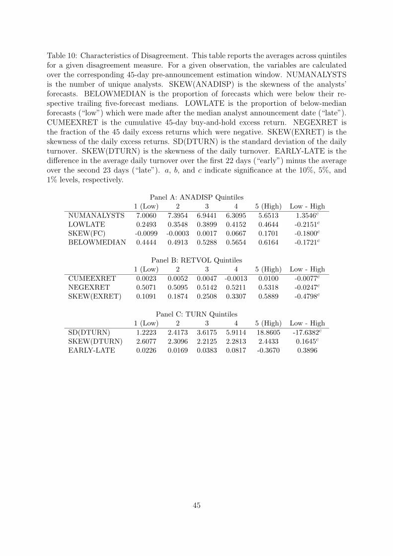
Table 10: Characteristics of Disagreement. This table reports the averages across quintilesfor a given disagreement measure. For a given observation, the variables are calculatedover the corresponding 45-day pre-announcement estimation window. NUMANALYSTSis the number of unique analysts. SKEW(ANADISP) is the skewness of the analysts’forecasts. BELOWMEDIAN is the proportion of forecasts which were below their re-spective trailing five-forecast medians. LOWLATE is the proportion of below-medianforecasts (“low”) which were made after the median analyst announcement date (“late”).CUMEEXRET is the cumulative 45-day buy-and-hold excess return. NEGEXRET isthe fraction of the 45 daily excess returns which were negative. SKEW(EXRET) is theskewness of the daily excess returns. SD(DTURN) is the standard deviation of the dailyturnover. SKEW(DTURN) is the skewness of the daily turnover. EARLY-LATE is thedifference in the average daily turnover over the first 22 days (“early”) minus the averageover the second 23 days (“late”). a, b, and c indicate significance at the 10%, 5%, and1% levels, respectively.

Panel A: ANADISP Quintiles1 (Low) 2 3 4 5 (High) Low - High

NUMANALYSTS 7.0060 7.3954 6.9441 6.3095 5.6513 1.3546c

LOWLATE 0.2493 0.3548 0.3899 0.4152 0.4644 -0.2151c

SKEW(FC) -0.0099 -0.0003 0.0017 0.0667 0.1701 -0.1800c

BELOWMEDIAN 0.4444 0.4913 0.5288 0.5654 0.6164 -0.1721c

Panel B: RETVOL Quintiles1 (Low) 2 3 4 5 (High) Low - High

CUMEEXRET 0.0023 0.0052 0.0047 -0.0013 0.0100 -0.0077c

NEGEXRET 0.5071 0.5095 0.5142 0.5211 0.5318 -0.0247c

SKEW(EXRET) 0.1091 0.1874 0.2508 0.3307 0.5889 -0.4798c

Panel C: TURN Quintiles1 (Low) 2 3 4 5 (High) Low - High

SD(DTURN) 1.2223 2.4173 3.6175 5.9114 18.8605 -17.6382c

SKEW(DTURN) 2.6077 2.3096 2.2125 2.2813 2.4433 0.1645c

EARLY-LATE 0.0226 0.0169 0.0383 0.0817 -0.3670 0.3896

45

0 1 2

Nothing happens.

The price is P0.

There is nodisagreement.

A public signalS = F + ε arrives,where ε ∼ (0, σε).

Analysts postforecasts xn ofF based on S.

Price P1 aggregatesthose forecasts.

F is realized.

The price isP2 = P0 + F

Figure 1: Timeline of the model

46

SDH

DL

PH

PL X

Figure 2: Inelastic supply and downward-sloping demand curves in the market for asecurity, per Miller (1977).

47

References

Abarbanell, J. S. (1991). Do analysts’ earnings forecasts incorporate information in prior

stock price changes? Journal of Accounting and Economics , 14 (2), 147–165.

Avramov, D., Chordia, T., Jostova, G., & Philipov, A. (2009). Dispersion in analysts’

earnings forecasts and credit rating. Journal of Financial Economics , 91 (1), 83–

101.

Berkman, H., Dimitrov, V., Jain, P. C., Koch, P. D., & Tice, S. (2009). Sell on the

news: Differences of opinion, short-sales constraints, and returns around earnings

announcements. Journal of Financial Economics , 92 (3), 376–399.

Brown, P., Foster, G., & Noreen, E. (1985). Security analyst multi-year earnings forecasts

and the capital market (No. 21). Amer Accounting Assn.

Carlin, B. I., Longstaff, F. A., & Matoba, K. (2014). Disagreement and asset prices.

Journal of Financial Economics , 114 (2), 226–238.

Cen, L., Wei, K. J., & Yang, L. (2016). Disagreement, underreaction, and stock returns.

Management Science, 63 (4), 1214–1231.

Collins, D. W., & Kothari, S. (1989). An analysis of intertemporal and cross-sectional

determinants of earnings response coefficients. Journal of accounting and economics ,

11 (2-3), 143–181.

David, A. (2008). Heterogeneous beliefs, speculation, and the equity premium. The

Journal of Finance, 63 (1), 41–83.

De Bondt, W. F., & Thaler, R. H. (1990). Do security analysts overreact? The American

Economic Review , 52–57.

Dechow, P. M., Hutton, A. P., & Sloan, R. G. (2000). The relation between analysts’

forecasts of long-term earnings growth and stock price performance following equity

offerings. Contemporary Accounting Research, 17 (1), 1–32.

Diether, K. B., Malloy, C. J., & Scherbina, A. (2002). Differences of opinion and the cross

section of stock returns. The Journal of Finance, 57 (5), 2113–2141.

48

Dreman, D. N., & Berry, M. A. (1995). Analyst forecasting errors and their implications

for security analysis. Financial Analysts Journal , 30–41.

Grinblatt, M., Jostova, G., & Philipov, A. (2017). Analyst bias and mispricing. working

paper .

Hong, H., Lim, T., & Stein, J. C. (2000). Bad news travels slowly: Size, analyst coverage,

and the profitability of momentum strategies. The Journal of Finance, 55 (1), 265–

295.

Hong, H., & Stein, J. C. (1999). A unified theory of underreaction, momentum trading,

and overreaction in asset markets. The Journal of finance, 54 (6), 2143–2184.

Johnson, T. C. (2004). Forecast dispersion and the cross section of expected returns. The

Journal of Finance, 59 (5), 1957–1978.

Kondor, P. (2012). The more we know about the fundamental, the less we agree on the

price. The Review of Economic Studies , 79 (3), 1175–1207.

Lahiri, K., & Sheng, X. (2008). Evolution of forecast disagreement in a bayesian learning

model. Journal of Econometrics , 144 (2), 325–340.

Lim, T. (2001). Rationality and analysts’ forecast bias. The Journal of Finance, 56 (1),

369–385.

Michaely, R., & Womack, K. L. (1999). Conflict of interest and the credibility of under-

writer analyst recommendations. Review of financial studies , 12 (4), 653–686.

Milgrom, P., & Stokey, N. (1982). Information, trade and common knowledge. Journal

of economic theory , 26 (1), 17–27.

Miller, E. M. (1977). Risk, uncertainty, and divergence of opinion. The Journal of finance,

32 (4), 1151–1168.

Scharfstein, D. S., & Stein, J. C. (1990). Herd behavior and investment. The American

Economic Review , 465–479.

Scherbina, A. (2008). Suppressed negative information and future underperformance.

Review of Finance, 533–565.

Stickel, S. E. (1990). Predicting individual analyst earnings forecasts. Journal of Ac-

49

counting Research, 409–417.

Trueman, B. (1994). Analyst forecasts and herding behavior. The Review of Financial

Studies , 7 (1), 97–124.

Tversky, A., & Kahneman, D. (1975). Judgment under uncertainty: Heuristics and biases.

In Utility, probability, and human decision making (pp. 141–162). Springer.

Varian, H. R. (1985). Divergence of opinion in complete markets: A note. The Journal

of Finance, 40 (1), 309–317.

Veenman, D., & Verwijmeren, P. (in press). Do investors fully unravel persistent pessimism

in analysts’ earnings forecasts? The Accounting Review .

Welch, I. (2000). Herding among security analysts. Journal of Financial economics ,

58 (3), 369–396.

Zhang, X. (2006). Information uncertainty and stock returns. The Journal of Finance,

61 (1), 105–137.

50