Embed Size (px)
Citation preview

Disaggregated Seismic Hazard and the Elastic Input Energy Spectrum:An Approach to Design Earthquake Selection
Martin C. Chapman
Thesis submitted to the Faculty of the Virginia Polytechnic Institute and State University in partial
fulfillment of the requirements for the degree of
Doctor of Philosophy
in
Geophysics
J. Arthur Snoke, Chair
Gilbert A. Bollinger
Edwin S. Robinson
James R. Martin
Mahendra P. Singh
June 25, 1998
Blacksburg, Virginia
Keywords: Seismic Hazard, Strong Motion, Design Earthquakes, Input Energy

Disaggregated Seismic Hazard and the Elastic Input Energy Spectrum: An
Approach to Design Earthquake Selection
Martin C. Chapman
(Abstract)
The design earthquake selection problem is fundamentally probabilistic. Disaggregation of aprobabilistic model of the seismic hazard offers a rational and objective approach that can identifythe most likely earthquake scenario(s) contributing to hazard. An ensemble of time series can beselected on the basis of the modal earthquakes derived from the disaggregation. This gives auseful time-domain realization of the seismic hazard, to the extent that a single motion parametercaptures the important time-domain characteristics. A possible limitation to this approach arisesbecause most currently available motion prediction models for peak ground motion or oscillatorresponse are essentially independent of duration, and modal events derived using the peak motionsfor the analysis may not represent the optimal characterization of the hazard.
The elastic input energy spectrum is an alternative to the elastic response spectrum for these typesof analyses. The input energy combines the elements of amplitude and duration into a singleparameter description of the ground motion that can be readily incorporated into standardprobabilistic seismic hazard analysis methodology. This use of the elastic input energy spectrum isexamined. Regression analysis is performed using strong motion data from Western NorthAmerica and consistent data processing procedures for both the absolute input energy equivalentvelocity, (Vea), and the elastic pseudo-relative velocity response (PSV) in the frequency range 0.5
to 10 Hz. The results show that the two parameters can be successfully fit with identical functionalforms. The dependence of Vea and PSV upon (NEHRP) site classification is virtually identical.The variance of Vea is uniformly less than that of PSV, indicating that Vea can be predicted with
slightly less uncertainty as a function of magnitude, distance and site classification. The effects ofsite class are important at frequencies less than a few Hertz. The regression modeling does notresolve significant effects due to site class at frequencies greater than approximately 5 Hz.
Disaggregation of general seismic hazard models using Vea indicates that the modal magnitudes for
the higher frequency oscillators tend to be larger, and vary less with oscillator frequency, thanthose derived using PSV. Insofar as the elastic input energy may be a better parameter forquantifying the damage potential of ground motion, its use in probabilistic seismic hazard analysiscould provide an improved means for selecting earthquake scenarios and establishing designearthquakes for many types of engineering analyses.

iii
Acknowledgments
I thank my graduate studies committee Drs. J. Arthur Snoke, Edwin S. Robinson, James R.
Martin, Mahendra P. Singh, and most of all, Dr. Gilbert A. Bollinger, for his long-term support
and guidance. Funding for these studies was provided by the Federal Emergency Management
Agency, the Virginia Department of Emergency Services, and the U. S. Geological Survey. The
Generic Mapping Tools software (Wessel and Smith, 1991) was used to prepare many of the
figures.

iv
Table of Contents
Acknowledgements................................................................................... iii
Table of Contents..................................................................................... iv
List of Figures........................................................................................ v
List of Tables.......................................................................................... vi
1. Introduction................................................................................... 1
2. Design Event Selection...................................................................... 3
2.1 Background.......................................................................... 3
2.2 Fundamentals of Probabilistic Hazard Analysis................................. 5
2.3 PSHA Disaggregation and the Modal Event..................................... 8
3. The Use of Elastic Input Energy for Design Event Selection........................... 19
3.1 Strong Motion Data................................................................. 19
3.2 Response Parameters............................................................... 22
3.2.1 Input Energy............................................................... 22
3.3 Regression Analysis................................................................ 24
3.3.1 Peak Acceleration, Velocity............................................... 24
3.3.2 PSV and Energy Spectra.................................................. 25
3.4 Implications for Seismic Hazard Assessment.................................... 26
4. Results and Conclusions.................................................................... 59
Bibliography........................................................................................... 61
Vita... . . . . . . . . . . . . . . . . . . . . . . . . . . . . . . . . . . . . . . . . . . . . . . . . . . . . . . . . . . . . . . . . . . . . . . . . . . . . . . . . . . . . . . . . . . . . . . . . . . . 64
v
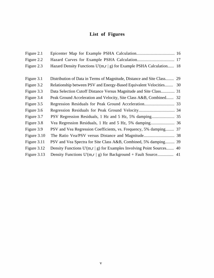
List of Figures
Figure 2.1 Epicenter Map for Example PSHA Calculation.................................. 16
Figure 2.2 Hazard Curves for Example PSHA Calculation................................. 17
Figure 2.3 Hazard Density Functions U'(m,r | g) for Example PSHA Calculation...... 18
Figure 3.1 Distribution of Data in Terms of Magnitude, Distance and Site Class........ 29
Figure 3.2 Relationship between PSV and Energy-Based Equivalent Velocities........ 30
Figure 3.3 Data Selection Cutoff Distance Versus Magnitude and Site Class............. 31
Figure 3.4 Peak Ground Acceleration and Velocity, Site Class A&B, Combined....... 32
Figure 3.5 Regression Residuals for Peak Ground Acceleration........................... 33
Figure 3.6 Regression Residuals for Peak Ground Velocity................................ 34
Figure 3.7 PSV Regression Residuals, 1 Hz and 5 Hz, 5% damping..................... 35
Figure 3.8 Vea Regression Residuals, 1 Hz and 5 Hz, 5% damping...................... 36
Figure 3.9 PSV and Vea Regression Coefficients, vs. Frequency, 5% damping........ 37
Figure 3.10 The Ratio Vea/PSV versus Distance and Magnitude............................ 38
Figure 3.11 PSV and Vea Spectra for Site Class A&B, Combined, 5% damping......... 39
Figure 3.12 Density Functions U'(m,r | g) for Examples Involving Point Sources....... 40
Figure 3.13 Density Functions U'(m,r | g) for Background + Fault Source............... 41

vi
List of Tables
Table 3.1 Strong Motion Recordings Used in Regression Analysis..................... 42
Table 3.2 NEHRP Site Classes............................................................... 49
Table 3.3 Regression Coefficients for PGA and PGV..................................... 50
Table 3.4 Regression Coefficients for PSV, 2% Damping................................ 51
Table 3.5 Regression Coefficients for PSV, 5% Damping................................ 52
Table 3.6 Regression Coefficients for PSV, 10% Damping............................... 53
Table 3.7 Regression Coefficients for Vea, 2% Damping................................. 54
Table 3.8 Regression Coefficients for Vea, 5% Damping................................. 55
Table 3.9 Regression Coefficients for Vea, 10% Damping................................ 56
Table 3.10 Modal Events for the Point Source Example..................................... 57
Table 3.11 Modal Events for the Combined Background and Line Source............... 68

1
Chapter 1: Introduction
The solution of many earthquake engineering problems involves dynamic analysis and testing
using ground motion time series. The time series, or design earthquake, should be selected to
reflect the characteristics of potential ground motions at a specific site. Important characteristics
include amplitude of motion, frequency content and duration of shaking. The characteristics are
determined by the earthquake source process, the wave propagation effects of the path between the
source and the site and the site response.
The design earthquake selection process involves consideration of the seismic hazard in the site
area and the general response characteristics of the structure(s) being analyzed. In most situations
the seismic hazard is uncertain, and is posed by the possible occurrence of earthquakes at more
than one location; likewise, the sizes, or magnitudes, of potentially damaging shocks may be
widely distributed. Distance and magnitude have a very important impact upon the nature of strong
motion at a specific site. Selecting time series for design is essentially a problem of choosing
appropriately from among a number of future earthquake scenarios. The most important elements
of the scenario are the magnitude of the earthquake and the distance from the source of energy
release to the site. Both of these elements are random variables: therefore, design earthquake
scenarios are best developed from a formal probabilistic model of the seismic hazard.
The research presented here addresses issues involved in the design earthquake selection
process. In Chapter 2, a probabilistic approach is presented that can provide an objective basis for
that selection. It offers the advantage that uncertainties can be accounted for quantitatively, and the
distinctions between competing interpretations of the seismic hazard can be readily examined. The
design earthquake scenarios are then derived using the concept of the modal event, which
represents the most likely combination of earthquake magnitude and source-site distance
contributing to the total hazard. To reflect the seismic hazard posed to complex structures, these
modal event scenarios are generated for a range of oscillator frequencies and damping values.
It is widely recognized that duration plays an important role in the damage potential of ground
motion for some types of construction. However, duration is not routinely modeled in
conventional probabilistic hazard analyses. In Chapter 3 of this study, the duration of shaking is
involved directly in the design earthquake selection through the use of a motion prediction model
based on elastic input energy. Empirical prediction models for pseudo-velocity and a parameter

2
based on elastic input energy are developed using the strong motion data set of western North
America and compared using consistent processing approaches. The prediction models are
developed for oscillator frequencies in the range 0.5 to 10 Hz, and for 3 values of damping. The
impact of the duration dependent parameter on the probabilistically developed scenario events is
assessed.
Chapter 4 concludes the study and presents a summary of results.
3
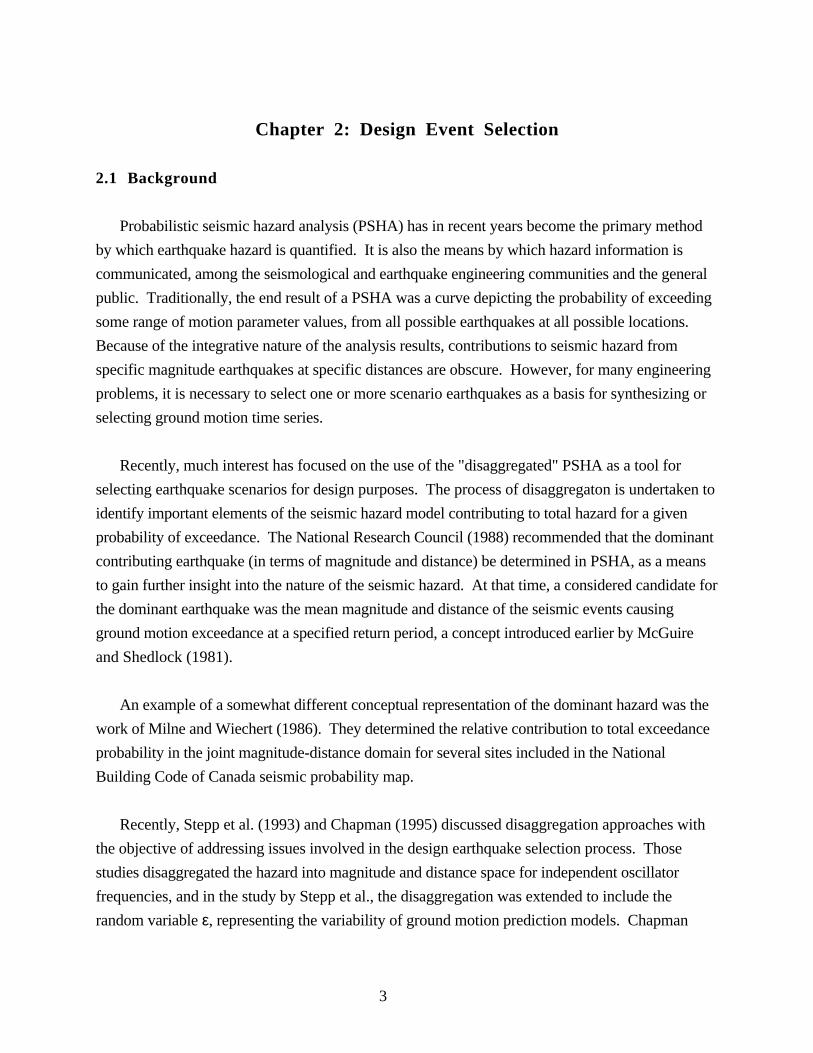
Chapter 2: Design Event Selection
2.1 Background
Probabilistic seismic hazard analysis (PSHA) has in recent years become the primary method
by which earthquake hazard is quantified. It is also the means by which hazard information is
communicated, among the seismological and earthquake engineering communities and the general
public. Traditionally, the end result of a PSHA was a curve depicting the probability of exceeding
some range of motion parameter values, from all possible earthquakes at all possible locations.
Because of the integrative nature of the analysis results, contributions to seismic hazard from
specific magnitude earthquakes at specific distances are obscure. However, for many engineering
problems, it is necessary to select one or more scenario earthquakes as a basis for synthesizing or
selecting ground motion time series.
Recently, much interest has focused on the use of the "disaggregated" PSHA as a tool for
selecting earthquake scenarios for design purposes. The process of disaggregaton is undertaken to
identify important elements of the seismic hazard model contributing to total hazard for a given
probability of exceedance. The National Research Council (1988) recommended that the dominant
contributing earthquake (in terms of magnitude and distance) be determined in PSHA, as a means
to gain further insight into the nature of the seismic hazard. At that time, a considered candidate for
the dominant earthquake was the mean magnitude and distance of the seismic events causing
ground motion exceedance at a specified return period, a concept introduced earlier by McGuire
and Shedlock (1981).
An example of a somewhat different conceptual representation of the dominant hazard was the
work of Milne and Wiechert (1986). They determined the relative contribution to total exceedance
probability in the joint magnitude-distance domain for several sites included in the National
Building Code of Canada seismic probability map.
Recently, Stepp et al. (1993) and Chapman (1995) discussed disaggregation approaches with
the objective of addressing issues involved in the design earthquake selection process. Those
studies disaggregated the hazard into magnitude and distance space for independent oscillator
frequencies, and in the study by Stepp et al., the disaggregation was extended to include the
random variable ε, representing the variability of ground motion prediction models. Chapman
4
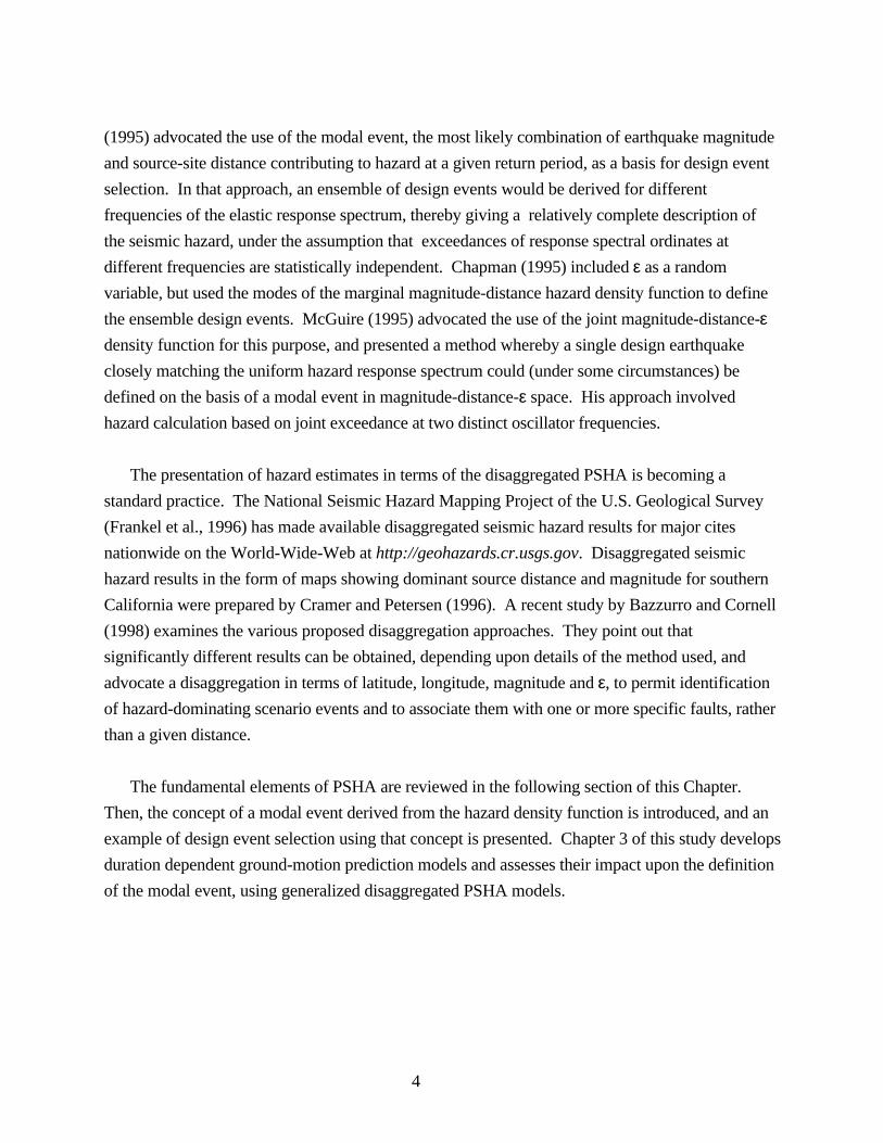
(1995) advocated the use of the modal event, the most likely combination of earthquake magnitude
and source-site distance contributing to hazard at a given return period, as a basis for design event
selection. In that approach, an ensemble of design events would be derived for different
frequencies of the elastic response spectrum, thereby giving a relatively complete description of
the seismic hazard, under the assumption that exceedances of response spectral ordinates at
different frequencies are statistically independent. Chapman (1995) included ε as a random
variable, but used the modes of the marginal magnitude-distance hazard density function to define
the ensemble design events. McGuire (1995) advocated the use of the joint magnitude-distance-εdensity function for this purpose, and presented a method whereby a single design earthquake
closely matching the uniform hazard response spectrum could (under some circumstances) be
defined on the basis of a modal event in magnitude-distance-ε space. His approach involved
hazard calculation based on joint exceedance at two distinct oscillator frequencies.
The presentation of hazard estimates in terms of the disaggregated PSHA is becoming a
standard practice. The National Seismic Hazard Mapping Project of the U.S. Geological Survey
(Frankel et al., 1996) has made available disaggregated seismic hazard results for major cites
nationwide on the World-Wide-Web at http://geohazards.cr.usgs.gov. Disaggregated seismic
hazard results in the form of maps showing dominant source distance and magnitude for southern
California were prepared by Cramer and Petersen (1996). A recent study by Bazzurro and Cornell
(1998) examines the various proposed disaggregation approaches. They point out that
significantly different results can be obtained, depending upon details of the method used, and
advocate a disaggregation in terms of latitude, longitude, magnitude and ε, to permit identification
of hazard-dominating scenario events and to associate them with one or more specific faults, rather
than a given distance.
The fundamental elements of PSHA are reviewed in the following section of this Chapter.
Then, the concept of a modal event derived from the hazard density function is introduced, and an
example of design event selection using that concept is presented. Chapter 3 of this study develops
duration dependent ground-motion prediction models and assesses their impact upon the definition
of the modal event, using generalized disaggregated PSHA models.

5
2.2 Fundamentals of Probabilistic Hazard Analysis
The method of quantifying seismic hazard has undergone much development and application
since being introduced by Cornell (1968). The objective of the probabilistic seismic hazard analysis
(PSHA) is to estimate the probability of exceeding a specified motion intensity, by taking into
account the potential occurrence of earthquakes at all possible locations, having all possible
magnitudes. Earthquake magnitude, source-site distance and motion intensity are the major
random variables in the PSHA.
A basic method common to most analyses is described below. A complete treatment of
statistical variability and uncertainty on all model parameters can be incorporated using Bayesian
estimation methods and Monte Carlo simulation (e.g., Coppersmith and Youngs, 1986; Bernreuter
et al., 1989; National Research Council, 1988). In the more sophisticated analyses, the basic
method may be performed several hundred to several thousand times, each time sampling the
model parameters from their distributions. In this way, the effects of random variability and model
uncertainty are quantified, in terms of a distribution function for exceedance probabilities.
In a conventional PSHA, exceedances of a specified motion intensity are assumed to follow the
Poisson stochastic process. The Poisson process is characterized by the following behavior: 1) an
event can occur at any time; 2) the occurrence of an event is independent of any other event, and 3)
the probability of an event occurring in a small time interval ∆t, is given by ν∆t, where ν is the
(constant) mean rate of occurrence. The Poisson process is defined by the Poisson probability
distribution:
P(Xt = x) =
(υt)x
x! e-υt for x=0,1,2...... (2.1)
where (P(Xt = x) is the probability of integer "x" events in time "t". For x=0, P(Xt = 0) = e-νt.
The probability of at least one event in time "t" is therefore given by
P(Xt ≠ 0) = 1 - e-υt . (2.2)
In a conventional PSHA, the task is to estimate νg, the mean rate of exceeding some motion
intensity g at a specific site. A general expression for νg is (Rieter, 1990; Chapman, 1995;
McGuire, 1995),
6
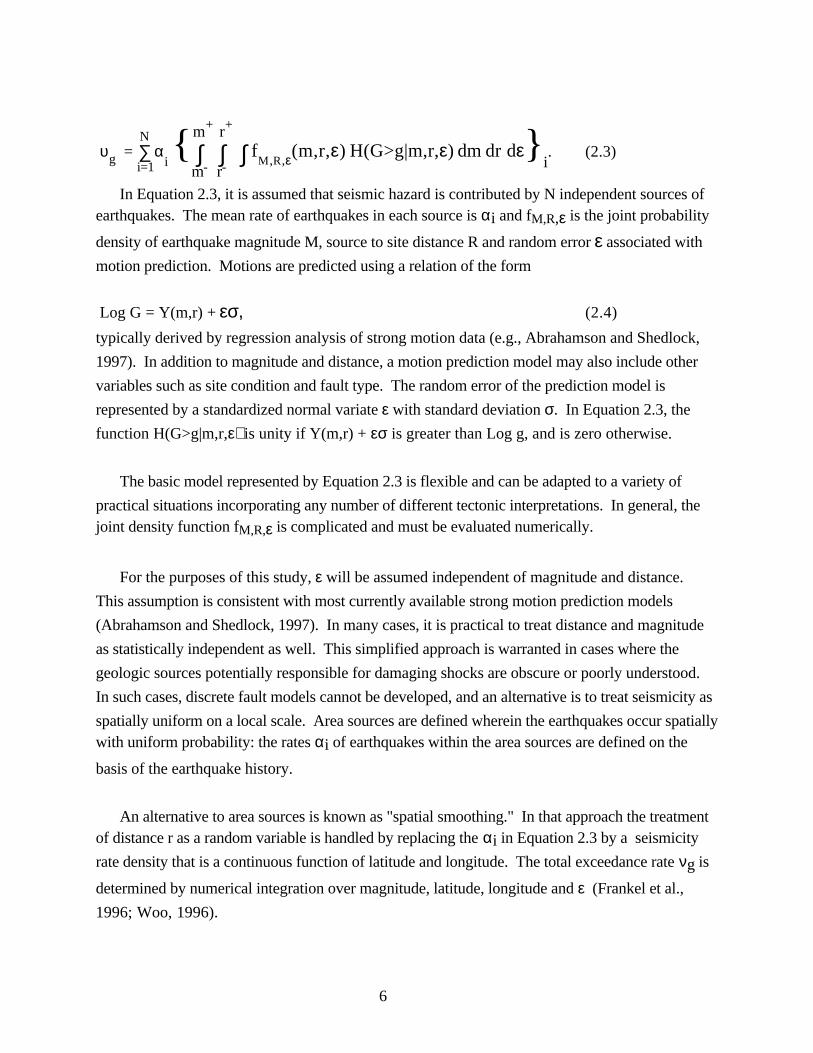
υg = ∑i=1
Nα
i { ∫
m-
m+
∫r-
r+
∫ fM,R,ε(m,r,ε) H(G>g|m,r,ε) dm dr dε}i. (2.3)
In Equation 2.3, it is assumed that seismic hazard is contributed by N independent sources ofearthquakes. The mean rate of earthquakes in each source is αi and fM,R,ε is the joint probability
density of earthquake magnitude M, source to site distance R and random error ε associated with
motion prediction. Motions are predicted using a relation of the form
Log G = Y(m,r) + εσ, (2.4)
typically derived by regression analysis of strong motion data (e.g., Abrahamson and Shedlock,
1997). In addition to magnitude and distance, a motion prediction model may also include other
variables such as site condition and fault type. The random error of the prediction model is
represented by a standardized normal variate ε with standard deviation σ. In Equation 2.3, the
function H(G>g|m,r,ε) is unity if Y(m,r) + εσ is greater than Log g, and is zero otherwise.
The basic model represented by Equation 2.3 is flexible and can be adapted to a variety of
practical situations incorporating any number of different tectonic interpretations. In general, thejoint density function fM,R,ε is complicated and must be evaluated numerically.
For the purposes of this study, ε will be assumed independent of magnitude and distance.
This assumption is consistent with most currently available strong motion prediction models
(Abrahamson and Shedlock, 1997). In many cases, it is practical to treat distance and magnitude
as statistically independent as well. This simplified approach is warranted in cases where the
geologic sources potentially responsible for damaging shocks are obscure or poorly understood.
In such cases, discrete fault models cannot be developed, and an alternative is to treat seismicity as
spatially uniform on a local scale. Area sources are defined wherein the earthquakes occur spatiallywith uniform probability: the rates αi of earthquakes within the area sources are defined on the
basis of the earthquake history.
An alternative to area sources is known as "spatial smoothing." In that approach the treatmentof distance r as a random variable is handled by replacing the αi in Equation 2.3 by a seismicity
rate density that is a continuous function of latitude and longitude. The total exceedance rate νg is
determined by numerical integration over magnitude, latitude, longitude and ε (Frankel et al.,
1996; Woo, 1996).

7
In situations where geologic evidence and/or the earthquake history warrants such treatment,
fault sources can be modeled (e.g., Bender, 1984). In more physically realistic models, fault
rupture length is dependent upon earthquake magnitude: as a result, source to site distance r
depends upon magnitude m.
For clarity in the present discussion, as well as in some examples that follow in later sections,
magnitude, distance and ε will be treated as statistically independent. It is important to recognize
that this assumption is not necessary, and does not limit the results and procedures of this study.
Also, for examples shown in this study, the hazard will be posed by discrete sources. A
formulation in terms of the spatial smoothing approach is straightforward. The issue of dependent
model parameters will be addressed in later sections, in the context of model disaggregation and
relevance to design earthquake selection.
Treating distance, magnitude and ε as statistically independent, the estimated rate of exceeding
motion intensity g due to hazard posed by N independent, discrete sources is
υg = ∑i=1
Nα
i { ∫
m-
m+
∫r-
r+
∫ fM(m)f
R(r)fε (ε)H(G>g|m,r,ε) dm dr dε}
i. (2.5)
The source-site distance probability density fR is defined by the spatial geometry of the source,
with respect to the site location. In this standard formulation, it is non-zero between limits of
integration r- and r+, representing the nearest and furthest approaches of an earthquake source to
the site.
The magnitude density fM depends upon the earthquake recurrence model. Often, fM is
assumed to be exponential, truncated at lower and upper limits of integration m- and m+: however,
that functional form is not a required assumption. The truncated exponential form of fM follows
from the empirical Gutenberg-Richter earthquake recurrence relationship, Log n = a-bm, relating n,
the rate of earthquakes with magnitudes exceeding m, to magnitude (Gutenberg and Richter,
1954). The upper magnitude truncation of the distribution reflects the constraint of finite release of
seismic energy. Another magnitude density function of interest is that related to the characteristic
earthquake model (Youngs and Coppersmith, 1985) which is used to model hazard from well-
documented active fault segments (e.g., Working Group for California Earthquake Probabilities,

8
1996; Frankel et al., 1996). The lower limit of magnitude integration, m-, is usually taken to be
approximately 4.5, representing the smallest earthquakes typically considered to be of engineering
concern. However, some care must be taken in specifying m-. As shown by Chapman (1995) m-
and g must be specified jointly such that Y(m-,r-) < Log g. Failure to satisfy this condition may
lead to significant underestimation of hazard. The upper magnitude truncation, m+, is a very
important parameter. Ideally, it is estimated using relevant geologic and paleoseismologic data,
geodetic strain rates and the seismic history of the region (Yeats et al., 1997; Working Group on
California Earthquake Probabilities, 1995). However, in most cases it is uncertain and may be
treated as a random variable in the hazard analysis (e.g., Bernreuter et al., 1989). For the
truncated exponential density function, fM is given by
fM
(m) = b' e-b'm
e-b'm-- e-b'm+ , m- < m < m+, (2.6)
where b' = ln(10)b. From Equations 2.3 and 2.5 it is clear that νg is proportional to the seismicity
rate α. The truncated exponential magnitude density, reflecting a constrained Gutenberg-Richter
earthquake recurrence model, implies
α = 10a-bm-
- 10a-bm
+
. (2.7)
Finally, it is assumed here that fε is the standard normal probability density function. It is
sometimes desirable to modify this distribution by truncating the tails and normalizing. This is
done to include the well-documented log-normal behavior of strong motion peak response values,
but limit the hazard model to motions that have been observed or that can reasonably be considered
possible on the basis of the empirical dataset. Typically, the density distribution is truncated at
approximately mean ± 2σ. That sort of model would imply lower and upper integration limits forε of -2 and +2 in Equations 2.3 and 2.5, and the necessary normalization of fε. In the examples
that follow, the untruncated standard normal distribution is used.
2.3 PSHA Disaggregation and the Modal Event
The identification of the events, in terms of magnitude and distance, that contribute most to
seismic hazard for a given probability of exceedance has practical application. It can serve as a
guide for defining scenarios and design earthquakes for engineering problems, particularly those
involving dynamic analysis using ground motion time series. For example, a user may wish to

9
select an actual strong-motion time series, that is in some sense "compatible" with a specific
probability of exceedance. This is a problem that in general has no unique deterministic solution.
As indicated by Equation 2.3, seismic hazard is the result of potential earthquakes that may exhibit
a range of magnitudes and may occur over a range of distances from a site. Clearly, the problem
of selecting one or more specific earthquake events, as required for some engineering applications,
is fundamentally probabilistic in nature. Therefore, a probabilistic approach to the decision process
is required.
As shown below, it is possible to identify the most likely (i.e., most frequent) events, defined
in terms of magnitude and distance, that contribute to seismic hazard. The information can be
obtained by "disaggregating" the results of a seismic hazard calculation. In the following, PSHA
disaggregation and modal event identification is discussed, and demonstrated using a simple
hypothetical example.
For simplicity, assume a hazard model wherein the random variables are statistically
independent and limited to those appearing in the motion prediction model (m, r and ε, Equation
2.4). For those conditions, Equation 2.5 completely defines the expected rate of exceeding a
specific motion intensity g.
Let U(m,r,ε | g) represent the integrand of Equation 2.5, for a specific value of g. This value g
could correspond to some chosen probability of exceedance: e.g., P(G>g)=0.001 (1000 year
return period). Thus,
U(m,r,ε | g) = ∑i=1
Nα
i {f
M(m)f
R(r)fε (ε)H(G>g|m,r,ε)}
i. (2.8)
Equation 2.8 represents the joint "hazard density" or "disaggregated hazard" for a specified
motion intensity g. In analogy to the definition of the mode of a random variable, let ( m , r , ε )define the location of the maximum value of U(m,r,ε | g). This is the "modal event" (or β-point;
McGuire, 1995) locating the mode of the joint hazard distribution for the exceedance of selected
motion value g. Integration with respect to the random variables yields the expected value of the
exceedance rate.
A marginal distribution U'(m,r | g) can be obtained by integration of Equation 2.8 with respect
to standardized random variable ε, or

10
U'(m,r | g) = ∫ U(m,r,ε | g) dε = ∑
i=1
N α
i { f
M(m) f
R(r) ∫
fε(ε) H(G>g|m,r,ε) dε}
i
= ∑i=1
N α
i { f
M(m) f
R(r) [1 - Φ(Log g - Y(m,r)
σ )]}i. (2.9)
In Equation 2.9, Φ is the cumulative normal probability distribution function. Let the
maximum value of U'(m,r | g) occur at ( m ' , r '). In general, m ' and r ' are not equivalent to m and r .
This is an important point. The magnitudes and distances of the modal events derived in the
disaggregation using marginal distributions may differ from those of the joint distribution. Most
recent work suggests that the appropriate disaggregation approach for design event selection is that
based on the joint hazard density function U(m,r,ε | g). Chapman (1995) advocated the use of the
marginal distribution U'(m,r | g) for this purpose because the physical significance of ε is that of a
scaling parameter that captures the effects of unmodeled physical processes. In actual practice, use
of U' to determine the modal magnitude m ' and distance r ' has an advantage in regard to the
scaling necessary to create a time series compatible with the specified motion g. On the other hand,
the modal magnitude m and distance r derived from U represents a "more likely" earthquake (in
terms of probability of occurring). This issue will be explored using an example calculation.
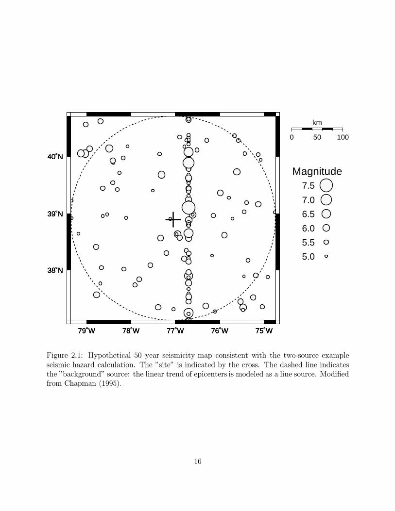
A hypothetical example is suggested by Figure 2.1, adapted from Chapman, (1995). One
approach could be to model the hazard using two independent sources: a line source with nearest
approach to the site of 30 km, and a "background" source area, enclosed by a circle of radius 200
km centered on the site. The example represents an active fault, embedded in a relatively less
seismic region. For both sources, we will assume the following recurrence relationship:
Log n = 4.101 - 0.8 m, (2.10)
where n is events per year, implying two magnitude 6 or greater earthquakes per decade within
each source. We will assume a truncated exponential density function for magnitude of the form of
Equation 2.6, where b' = 0.8 ln(10). For the line source, let m- = 5.0 and m+ = 7.7. In the
background, let m- = 5.0 and m+ = 6.5. The expected rate α of earthquakes with magnitudes
between m- and m+ is given by Equation 2.7.
The probability density of epicentral distance for the background source is
11
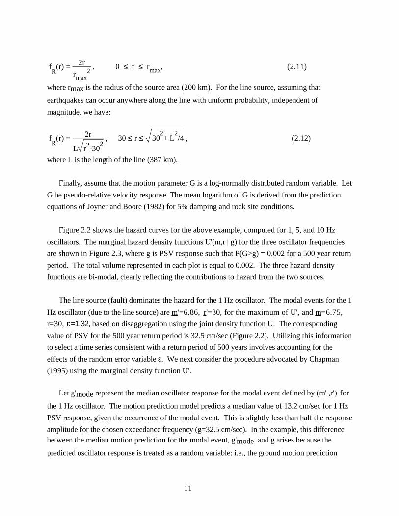
fR
(r) = 2r
rmax2 , 0 ≤ r ≤ rmax, (2.11)
where rmax is the radius of the source area (200 km). For the line source, assuming that
earthquakes can occur anywhere along the line with uniform probability, independent of
magnitude, we have:
fR
(r) = 2r
L r2-302
, 30 ≤ r ≤ 302+ L
2/4 , (2.12)
where L is the length of the line (387 km).
Finally, assume that the motion parameter G is a log-normally distributed random variable. Let
G be pseudo-relative velocity response. The mean logarithm of G is derived from the prediction
equations of Joyner and Boore (1982) for 5% damping and rock site conditions.
Figure 2.2 shows the hazard curves for the above example, computed for 1, 5, and 10 Hz
oscillators. The marginal hazard density functions U'(m,r | g) for the three oscillator frequencies
are shown in Figure 2.3, where g is PSV response such that P(G>g) = 0.002 for a 500 year return
period. The total volume represented in each plot is equal to 0.002. The three hazard density
functions are bi-modal, clearly reflecting the contributions to hazard from the two sources.
The line source (fault) dominates the hazard for the 1 Hz oscillator. The modal events for the 1
Hz oscillator (due to the line source) are m '=6.86, r '=30, for the maximum of U', and m =6.75,
r =30, ε =1.32, based on disaggregation using the joint density function U. The corresponding
value of PSV for the 500 year return period is 32.5 cm/sec (Figure 2.2). Utilizing this information
to select a time series consistent with a return period of 500 years involves accounting for the
effects of the random error variable ε. We next consider the procedure advocated by Chapman
(1995) using the marginal density function U'.
Let g'mode represent the median oscillator response for the modal event defined by ( m ' , r ') for
the 1 Hz oscillator. The motion prediction model predicts a median value of 13.2 cm/sec for 1 Hz
PSV response, given the occurrence of the modal event. This is slightly less than half the response
amplitude for the chosen exceedance frequency (g=32.5 cm/sec). In the example, this differencebetween the median motion prediction for the modal event, g'mode, and g arises because the
predicted oscillator response is treated as a random variable: i.e., the ground motion prediction
12
model includes the random variable ε. This element of the seismic hazard model complicates the
problem of design event selection, but is necessary because motion intensity at a given distance
from an earthquake exhibits statistical variation or "scatter", here represented by ε. Although the
scatter associated with a particular motion prediction model can, in principle, be reduced by
modeling additional information on the earthquake source, propagation path and site response, it
cannot be eliminated entirely. A significant reduction in the scatter is particularly difficult when the
locations and magnitudes (and associated source and path effects) of future earthquakes are
uncertain.
In the example, the base 10 logarithm of oscillator response is assumed to be normally
distributed with σ = 0.33. The logarithm of oscillator response corresponding to P(G>g) = 0.002
is approximately 1.18 standard deviations above the predicted mean logarithm of response for the
modal event ( m ' , r '). Therefore, given the occurrence of the modal event, there is approximately a
12% probability that the resulting PSV response at the site will exceed g = 32.5 cm/sec, for
P(G>g) = 0.002. For dynamic analyses at frequencies near 1 Hz, a ground motion time series
consistent with the results of the example hazard analysis could be selected at the 88% percentile
from the population of time series recorded at r '=30 km from magnitude m '=6.86 earthquakes.
Because this population is small, a more practical approach is to select or synthesize a "best
estimate" ground motion time series representative of the modal event, and scale the amplitude of
the time series such that the PSV response is g=32.5 cm/sec corresponding to the design P(G>g).
It is important to note that this approach is strictly valid only for a narrow frequency band.Further, as shown by Chapman (1995), the interpretation of the difference between g'mode and g
as due entirely to the modeling of random scatter in the motion prediction model holds only for
hazard models wherein three conditions are satisfied. First, the partial derivative with respect to
magnitude of the joint hazard density function U'(m,r) of each source contributing to hazard at agiven site must be negative: i.e., fM(m)fR(r) or fR,M(m,r) for each source must decrease with
increasing magnitude. This condition is always satisfied for the common situation where distance
and magnitude can be treated as statistically independent and the magnitude density functions of the
various sources are assumed exponential. However, a subset of the group of models wherein
distance and magnitude are statistically dependent may not satisfy this condition in all cases. Thesecond condition, implied by Equation 2.9, is that fε(ε)H(G>g|m,r,ε) remain invariant among the
sources contributing to hazard. This amounts to using the same attenuation model Y(m,r) and εdistribution function to predict ground motion for each source. Finally, the third condition is that
13
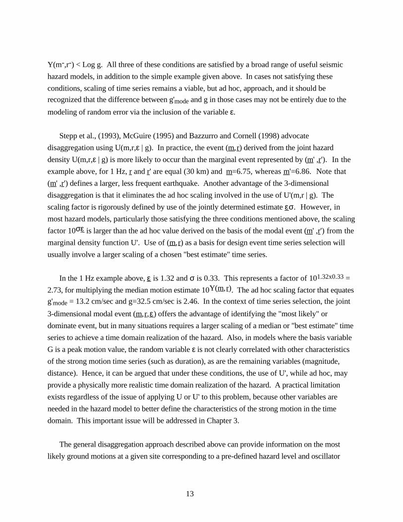
Y(m-,r-) < Log g. All three of these conditions are satisfied by a broad range of useful seismic
hazard models, in addition to the simple example given above. In cases not satisfying these
conditions, scaling of time series remains a viable, but ad hoc, approach, and it should be
recognized that the difference between g'mode and g in those cases may not be entirely due to the
modeling of random error via the inclusion of the variable ε.
Stepp et al., (1993), McGuire (1995) and Bazzurro and Cornell (1998) advocate
disaggregation using U(m,r,ε | g). In practice, the event ( m , r ) derived from the joint hazard
density U(m,r,ε | g) is more likely to occur than the marginal event represented by ( m ' , r '). In the
example above, for 1 Hz, r and r ' are equal (30 km) and m =6.75, whereas m '=6.86. Note that
( m ' , r ') defines a larger, less frequent earthquake. Another advantage of the 3-dimensional
disaggregation is that it eliminates the ad hoc scaling involved in the use of U'(m,r | g). The
scaling factor is rigorously defined by use of the jointly determined estimate ε σ. However, in
most hazard models, particularly those satisfying the three conditions mentioned above, the scaling
factor 10σε is larger than the ad hoc value derived on the basis of the modal event ( m ' , r ') from the
marginal density function U'. Use of ( m , r ) as a basis for design event time series selection will
usually involve a larger scaling of a chosen "best estimate" time series.
In the 1 Hz example above, ε is 1.32 and σ is 0.33. This represents a factor of 101.32x0.33 =
2.73, for multiplying the median motion estimate 10Y(m,r ). The ad hoc scaling factor that equates
g'mode = 13.2 cm/sec and g=32.5 cm/sec is 2.46. In the context of time series selection, the joint
3-dimensional modal event ( m , r , ε ) offers the advantage of identifying the "most likely" or
dominate event, but in many situations requires a larger scaling of a median or "best estimate" time
series to achieve a time domain realization of the hazard. Also, in models where the basis variable
G is a peak motion value, the random variable ε is not clearly correlated with other characteristics
of the strong motion time series (such as duration), as are the remaining variables (magnitude,
distance). Hence, it can be argued that under these conditions, the use of U', while ad hoc, may
provide a physically more realistic time domain realization of the hazard. A practical limitation
exists regardless of the issue of applying U or U' to this problem, because other variables are
needed in the hazard model to better define the characteristics of the strong motion in the time
domain. This important issue will be addressed in Chapter 3.
The general disaggregation approach described above can provide information on the most
likely ground motions at a given site corresponding to a pre-defined hazard level and oscillator
14
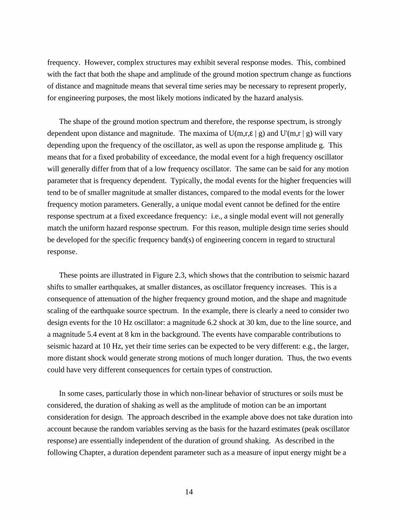
frequency. However, complex structures may exhibit several response modes. This, combined
with the fact that both the shape and amplitude of the ground motion spectrum change as functions
of distance and magnitude means that several time series may be necessary to represent properly,
for engineering purposes, the most likely motions indicated by the hazard analysis.
The shape of the ground motion spectrum and therefore, the response spectrum, is strongly
dependent upon distance and magnitude. The maxima of U(m,r,ε | g) and U'(m,r | g) will vary
depending upon the frequency of the oscillator, as well as upon the response amplitude g. This
means that for a fixed probability of exceedance, the modal event for a high frequency oscillator
will generally differ from that of a low frequency oscillator. The same can be said for any motion
parameter that is frequency dependent. Typically, the modal events for the higher frequencies will
tend to be of smaller magnitude at smaller distances, compared to the modal events for the lower
frequency motion parameters. Generally, a unique modal event cannot be defined for the entire
response spectrum at a fixed exceedance frequency: i.e., a single modal event will not generally
match the uniform hazard response spectrum. For this reason, multiple design time series should
be developed for the specific frequency band(s) of engineering concern in regard to structural
response.
These points are illustrated in Figure 2.3, which shows that the contribution to seismic hazard
shifts to smaller earthquakes, at smaller distances, as oscillator frequency increases. This is a
consequence of attenuation of the higher frequency ground motion, and the shape and magnitude
scaling of the earthquake source spectrum. In the example, there is clearly a need to consider two
design events for the 10 Hz oscillator: a magnitude 6.2 shock at 30 km, due to the line source, and
a magnitude 5.4 event at 8 km in the background. The events have comparable contributions to
seismic hazard at 10 Hz, yet their time series can be expected to be very different: e.g., the larger,
more distant shock would generate strong motions of much longer duration. Thus, the two events
could have very different consequences for certain types of construction.
In some cases, particularly those in which non-linear behavior of structures or soils must be
considered, the duration of shaking as well as the amplitude of motion can be an important
consideration for design. The approach described in the example above does not take duration into
account because the random variables serving as the basis for the hazard estimates (peak oscillator
response) are essentially independent of the duration of ground shaking. As described in the
following Chapter, a duration dependent parameter such as a measure of input energy might be a

15
more useful basis variable for the hazard analysis. An approach similar to that discussed
previously could be performed to identify the modal events and select appropriate time series,
provided that the duration dependent parameter is predictable as a function of magnitude and
distance.
79˚W 78˚W 77˚W 76˚W 75˚W
38˚N
39˚N
40˚N
0 50 100
km
79˚W 78˚W 77˚W 76˚W 75˚W
38˚N
39˚N
40˚N
79˚W 78˚W 77˚W 76˚W 75˚W
38˚N
39˚N
40˚N
79˚W 78˚W 77˚W 76˚W 75˚W
38˚N
39˚N
40˚N
Magnitude7.5
7.0
6.5
6.0
5.5
5.0
Figure 2.1: Hypothetical 50 year seismicity map consistent with the two-source exampleseismic hazard calculation. The ”site” is indicated by the cross. The dashed line indicatesthe ”background” source: the linear trend of epicenters is modeled as a line source. Modifiedfrom Chapman (1995).
16

0.0001
0.0010.001
0.01
0.1
0 10 20 30 40 50 60
PSV (cm/sec)
Exc
eeda
nce
Fre
quen
cy (
1/yr
)
10 Hz
0.0001
0.0010.001
0.01
0.1
0 10 20 30 40 50 60
PSV (cm/sec)
5 Hz
0.0001
0.0010.001
0.01
0.1
0 10 20 30 40 50 60
PSV (cm/sec)
1 Hz
Figure 2.2: Seismic hazard curves, (PSV response) for the example discussed in the text.Modified from Chapman (1995).
17

0
20
40
60 5.05.5
6.06.5
7.07.5
0.0
00
20
.00
04
0.0
00
20
.00
04
1 Hz
0
20
40
60 5.05.5
6.06.5
7.07.5
0.0
00
20
.00
04
De
nsi
ty
0.0
00
20
.00
04
De
nsi
ty
5 Hz
0
20
40
60
Distance (Km)5.0
5.56.0
6.57.0
7.5
Magnitude
0.0
00
20
.00
04
0.0
00
20
.00
04
10 Hz
Figure 2.3: Marginal hazard density functions U’ for the example discussed in the text.The three functions are for a return period of 500 years, for PSV response. Note that asoscillator frequency increases, the relative contribution to hazard shifts to smaller magnitudesand distances. Modified from Chapman (1995).
18
19
Chapter 3: The Use of Elastic Input Energy forDesign Event Selection
The probabilistic seismic hazard analysis requires a model from which median estimates of a
strong motion parameter can be derived as a function of magnitude, distance and perhaps other
variables such as site condition and type of faulting. The model must provide an estimate of the
statistical variability of the parameter. Most suitable motion prediction models currently available
yield estimates of peak ground motion values or peak response of elastic, single-degree-of-freedom
(SDOF) oscillators: e.g., pseudo-relative velocity (PSV) response. Such measures of motion are
essentially independent of the duration of the ground motion. As a result, scenario events derived
from them do not necessarily represent the optimum events to be used for some types of
engineering design studies.
This section of the study examines the potential use of a parameter derived from the elastic
input energy spectrum for probabilistic seismic hazard analysis. The input energy reflects the
duration of ground shaking directly through time domain integration, and for that reason could
potentially provide an improved basis for defining scenario events. A recent comprehensive study
by Lawson (1996) developed regression models for both elastic and inelastic input energy spectra,
as well as elastic response spectra. The present study uses a similar, but somewhat larger, data set,
comprised of western North American strong motion recordings.
The focus of this Chapter is on a comparison of the magnitude and distance dependence of the
elastic input energy spectrum with the elastic PSV response spectrum which is commonly used in
probabilistic hazard analysis. The objective is to assess the degree to which use of a duration
dependent motion parameter changes the results with respect to the type of earthquakes (magnitude
and distance) that contribute to hazard at a given probability level. This is done by first developing
representative motion prediction models for the two parameters using identical data processing
procedures, and then comparing the disaggregated results of simple, but fairly general seismic
hazard models.
3.1 Strong Motion Data
The data set used in this study consists of horizontal component recordings from 23
earthquakes in western North America. Table 3.1 lists the earthquakes, along with station names
20
and site numbers, component azimuth, source to site distance, station coordinates and site
classification. The source to station distance adopted for this study is that used by Boore et al.,
(1993, 1994 and 1997), and is the nearest horizontal distance from the station to the surface
projection of the fault rupture. The site classification is that adopted by the NEHRP, (BSSC,
1994; see also Boore et al., 1997) which is defined on the basis of average shear wave velocity in
the upper 30 meters (Table 3.2).
Data selection and regression modeling used in this study follows closely the approach
developed and used in previous work by Boore et al., (1993, 1994, 1997) and Joyner and Boore
(1993, 1994). The data used here were recorded at ground level or in basements of structures of
two stories or less, and do not include data from dam or bridge abutments. For 17 of the 23
earthquakes, the data assembled here for analysis is a subset of that used and documented
thoroughly by Boore et al. (1993, 1994 and 1997). The remaining data are recordings from the
1994 Northridge shock and from some recent shocks with magnitudes in the range 5.0 to 6.2
(Westmoreland, Morgan Hill, Whittier Narrows, Sierra Madre, and Big Bear).
The sources of strong motion data were the collection of recordings assembled and distributed
by NOAA (Earthquake Strong Motion CD-ROM); and the internet websites maintained by the
California Division of Mines and Geology strong motion instrumentation program, the U. S.
Geological Survey national strong motion program and the Civil Engineering Department,
University of Southern California. Table 3.1 identifies the source of the data, along with that
organization's site identification number, as appearing in the data file header, if available.
The recordings were selected so as to include the entire S-wavetrain. Recordings that triggered
late on the S wave, or those of short duration terminating early in the coda, were not used. The
iterative approach described by Campbell (1997) was used to avoid bias due to the effects of non-
triggered instruments, in the data sets from some of the more recent shocks. This will be
discussed further below.
Corrected accelerogram data provided by the contributing sources comprise a large portion of
the assembled data set. However, a sizable fraction of the data was processed by the author for
this study. Evenly sampled, uncorrected data were available from the U. S. Geological Survey
National Strong Motion Program (NSMP) for the Petrolia, Landers, Big Bear and Northridge
earthquakes. Those data were instrument corrected and bandpassed using a 4-pole causal

21
Butterworth filter with corner frequencies 0.1 and 25 Hz. Unevenly sampled, uncorrected data
were available from the University of Southern California (USC) sites for the Whittier Narrows,
Sierra Madre, Landers, Big Bear and Northridge earthquakes. Those data were interpolated and
sampled evenly using a 0.005 s interval, and instrument corrected. A causal Butterworth bandpass
filter with corner frequencies at 0.2 and 25 Hz was then applied. A 6-pole filter was used for the
Landers and Big Bear data, whereas a 4-pole filter was used for the Whittier Narrows and Sierra
Madre recordings.
In all cases, using corrected data from the contributing sources or data corrected as described
above, the recordings were passed through a final filter stage consisting of a 6-pole, causal high-
pass Butterworth filter, with corner frequency 0.2 Hz. The filter parameter selections were chosen
to insure that low-frequency noise was suppressed. This was verified for all the data by visual
inspection of integrated velocity and displacement recordings. The response and energy spectra
derived from these data are considered reliable for oscillator frequencies greater than 0.5 Hz.
Site classification according to BSSC (1994) for the recording sites listed in Table 3.1 was
obtained from compilations of Boore et al., (1993), Harmsen (1997) and Boore et al., (1997).
Source to recording site distances for all earthquakes occurring prior to 1981, as well as for the
Loma Prieta and Petrolia earthquakes, are taken from Boore et al., (1993, 1997). Site distances
for the Westmoreland earthquake were calculated using the aftershock distribution as given by
Sharp et al. (1986). Distances for the Morgan Hill earthquake were calculated from the aftershock
distribution summarized by Cockerham and Eaton (1987). The aftershock distributions given by
Hauksson (1994) were used to calculate the site distances for the Whittier Narrows and Sierra
Madre earthquakes. Distances for the Landers and Big Bear earthquakes were derived from the
aftershock distributions and the fault model of Wald and Heaton (1994). Distances for the
Northridge earthquake were derived using the rupture model of Wald et al., (1996).
Figure 3.1 shows the distribution of data in terms of magnitude, distance and site
classification. Site classes A and B (Table 3.2) are combined for analysis, because so few data are
available.

22
3.2 Response Parameters
The emphasis of this study in on comparing the distance and magnitude dependence of
maximum elastic oscillator response and of input energy. Regression analysis is performed on
peak horizontal ground acceleration (PGA), peak horizontal ground velocity (PGV), elastic
oscillator pseudo-relative velocity response (PSV) and a parameter derived from the absolute input
energy for elastic oscillators. The regression models are derived for a randomly oriented horizontal
component, using the geometric mean of the two horizontal components.
The values of PGA and PGV used in this study are those values obtained from the corrected
acceleration and integrated corrected acceleration recordings, following filtering as described
above. Note that a small difference exists in the values of those parameters used in regression and
the values of the original recordings.
The algorithm of Nigam and Jennings (1969) was used to calculate the elastic oscillator
response time series necessary for construction of PSV and energy spectra.
3.2.1 Input Energy
Following Uang and Bertero (1990), the equation of motion of a damped SDOF system is
m (x..
g+ x..) + c x
. +f = 0 (3.1)
Here, xg is the displacement of the ground, and x is the relative displacement of the mass with
respect to the ground, c is the damping coefficient and f is the restoring force. The equation ofmotion of an equivalent system with fixed base, acted upon by a force -m x
..g is given by
m x.. + c x
. +f = -mx
..g . (3.2)
Uang and Bertero (1990) show that the equivalent representations of the dynamic system lead
to two definitions of input energy. Integrating Equation 3.1 with respect to x leads to
m x.t
2/2 +∫ cx
. dx +∫ f dx = ∫ m x
..t dxg , (3.3)
where xt=xg+x, is the total or absolute displacement. Integration of Equation 3.2 with respect to x
leads to
23
m x. 2
/2 +∫ cx. dx +∫ f dx = -∫ m x
..g dx . (3.4)
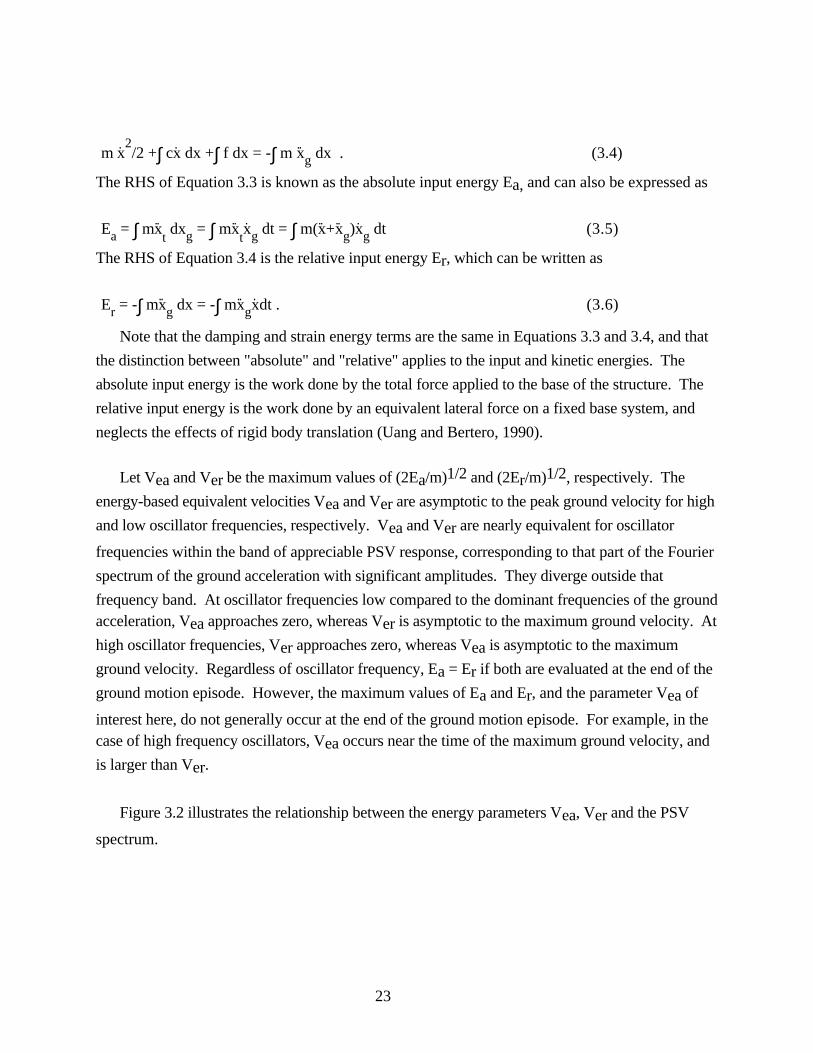
The RHS of Equation 3.3 is known as the absolute input energy Ea, and can also be expressed as
Ea = ∫ mx..
t dxg = ∫ mx
..tx.g dt = ∫ m(x
..+x
..g)x
.g dt (3.5)
The RHS of Equation 3.4 is the relative input energy Er, which can be written as
Er = -∫ mx..
g dx = -∫ mx..
gx.dt . (3.6)
Note that the damping and strain energy terms are the same in Equations 3.3 and 3.4, and that
the distinction between "absolute" and "relative" applies to the input and kinetic energies. The
absolute input energy is the work done by the total force applied to the base of the structure. The
relative input energy is the work done by an equivalent lateral force on a fixed base system, and
neglects the effects of rigid body translation (Uang and Bertero, 1990).
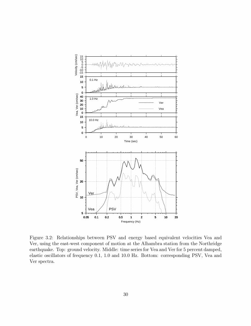
Let Vea and Ver be the maximum values of (2Ea/m)1/2 and (2Er/m)1/2, respectively. The
energy-based equivalent velocities Vea and Ver are asymptotic to the peak ground velocity for high
and low oscillator frequencies, respectively. Vea and Ver are nearly equivalent for oscillator
frequencies within the band of appreciable PSV response, corresponding to that part of the Fourier
spectrum of the ground acceleration with significant amplitudes. They diverge outside that
frequency band. At oscillator frequencies low compared to the dominant frequencies of the groundacceleration, Vea approaches zero, whereas Ver is asymptotic to the maximum ground velocity. At
high oscillator frequencies, Ver approaches zero, whereas Vea is asymptotic to the maximum
ground velocity. Regardless of oscillator frequency, Ea = Er if both are evaluated at the end of the
ground motion episode. However, the maximum values of Ea and Er, and the parameter Vea of
interest here, do not generally occur at the end of the ground motion episode. For example, in thecase of high frequency oscillators, Vea occurs near the time of the maximum ground velocity, and
is larger than Ver.
Figure 3.2 illustrates the relationship between the energy parameters Vea, Ver and the PSV
spectrum.

24
3.3 Regression Analysis
The following regression model (Boore et al., 1993) is fitted to the PSV and Vea data sets, and
to the peak ground acceleration (PGA) and velocity (PGV) data.
Log10 Y = a + b(M-6) + c(M-6)2 + d log (r2 + h2)1/2 + e G1 + f G2 + ε. (3.7)
Here, Y is the response variable (the geometric mean of the two horizontal components), expressed
in units of centimeters and seconds, M is moment magnitude, r is the horizontal distance, in km, to
the nearest surface projection of the fault rupture, and G1 and G2 are indicator variables for site
classifications C and D (e.g.: G1=1 for class C sites, 0 otherwise, G2 = 1 for class D sites, 0
otherwise). The unknowns a,b,c,d,h,e,f and the variance σ2 of random error ε are determined
using the two-step regression procedure of Joyner and Boore (1993, 1994).
The normally distributed error term ε has zero mean and standard deviation σ composed of
two components, such that σ2 = σr2 + σe2. The variance σr2 is associated with the first stage
of the regression wherein the unknowns d, h, e and f are estimated, along with "amplitude factors"
for each of the earthquakes. The variance σe2 is that associated with the second stage regression
wherein the amplitude factors are regressed against magnitude. For the model of a randomly
oriented horizontal component, the response Y is the geometric mean of the two horizontal
components, and the estimate of σr2 must be increased to account for the variance associated with
choosing one of the components randomly (Boore et al., 1993).
3.3.1 Peak Acceleration, Velocity
To avoid bias due to non-triggered stations, the PGA regression model was developed
iteratively, as described by Campbell (1997). In the first step, the entire assembled data set was
used to determine a set of minimum distances at which the 16th percentile values of the model is
less than 0.02 g, corresponding to a 0.01g vertical component trigger threshold. These distances
are functions of magnitude and site condition. Next, corresponding data points at larger distances
were deleted and the regression was repeated. One iteration was sufficient to eliminate potentially
biased data points, based on the 16th percentile criterion. The remaining data (Table 3.1) were
25
then used in all further regressions of PGA, PGV, PSV and the energy-based equivalent velocityVea. Figure 3.3 plots the minimum cutoff distances as a function of magnitude and site class.
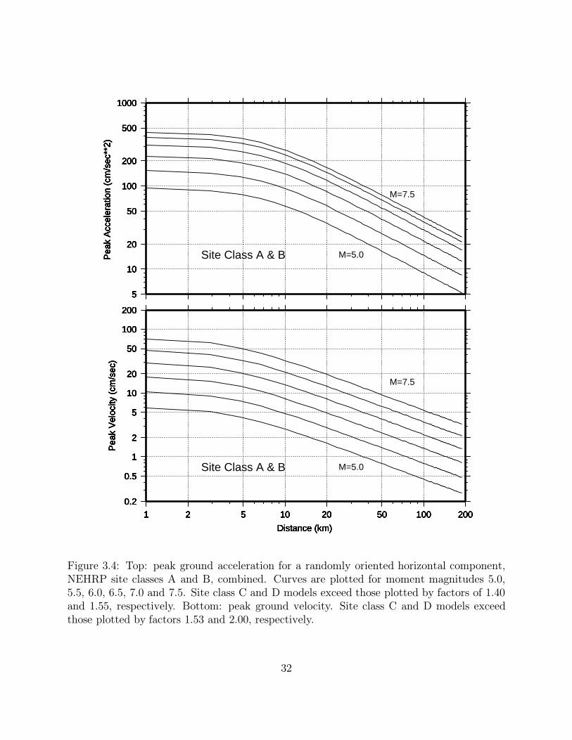
Table 3.3 lists the results of the regression analysis for peak ground acceleration (PGA) and
velocity (PGV). Figure 3.4 plots the models for the randomly oriented horizontal component, for
the combined site classes A & B, as a function of magnitude and distance. Figures 3.5 and 3.6
show the regression residuals as functions of distance and magnitude. Figure 3.4 suggests that
PGA undergoes saturation for M>6.5. Also, the effect of site classification is larger for PGV than
for PGA. Regression coefficients e and f for PGA correspond to amplification factors of 1.40 and
1.55 for site classes C and D, respectively. These amplification factors have values of 1.53 and
2.00, respectively, for PGV. Figures 3.5 and 3.6 show that Equation 3.7 does a good job overall
of fitting the PGA and PGV data, with no obvious non-normal magnitude or distance dependent
trends apparent in the residual plots. The data scatter for PGV is somewhat larger than for PGA.
3.3.2 PSV and Energy Spectra
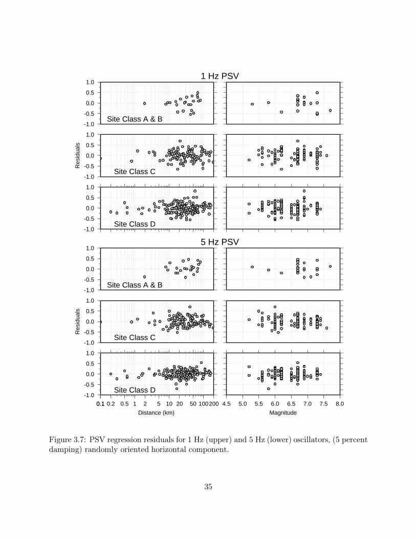
Tables 3.4 through 3.6 list regression results for PSV for 3 values of damping (2%, 5% and10% critical). Tables 3.7 through 3.9 list corresponding results for Vea. Figure 3.7 shows
residuals versus distance and magnitude for oscillator frequencies 1 Hz and 5 Hz. Figure 3.8
shows corresponding residual plots for Vea.
The residuals show no obvious magnitude or distance dependent trends, and it is apparent thatthe regression model Equation 3.7 is equally appropriate for PSV and Vea. Figures 3.7 and 3.8
are representative of results obtained for other frequency and damping values.
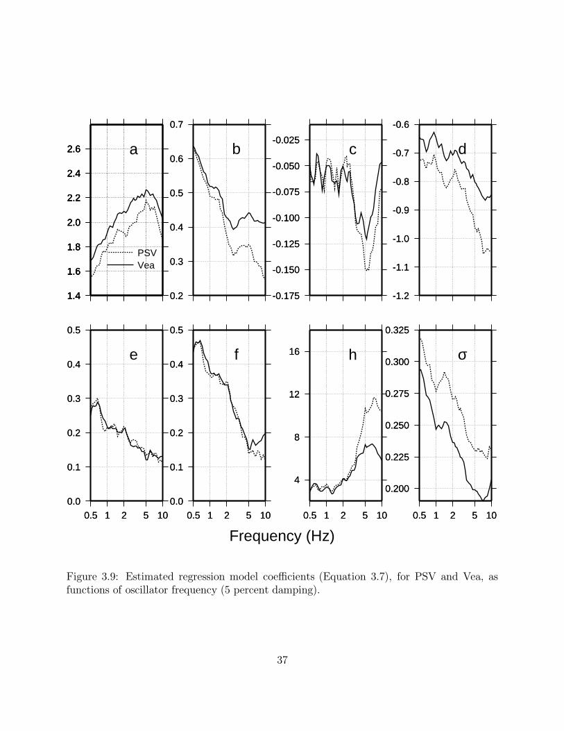
Figure 3.9 compares the regression coefficients versus frequency for Vea and PSV at 5%
damping. The linear magnitude coefficient "b" is significantly larger (more positive) for theenergy-based parameter Vea than for PSV, at the higher frequencies, indicating a stronger high-
frequency scaling of Vea with magnitude. The distance coefficient "d" is also more positive for
Vea, indicating a tendency for less distance attenuation of the parameter, compared to PSV, at all
frequencies. The parameter "h", which functions as a pseudo-focal depth term, is nearly the samefor Vea and PSV for frequencies less than about 3 Hz. At higher frequencies, h for PSV exceeds
that for Vea. The site class coefficients "e" and "f" are very similar for Vea and PSV. In both
cases, the effect of site class is most important at the lower frequencies. The effects of site class

26
are unresolved by the regression analysis at frequencies greater than 5 Hz. Finally, the standard
deviation of the regression, σ, generally decreases with increasing oscillator frequency, and isuniformly smaller for Vea than for PSV, as can be seen from a comparison of Figures 3.7 and 3.8.
The results just described are much the same for the 2% and 10% damped oscillators.
The relative magnitude and distance dependence of PSV and Vea is illustrated in Figure 3.10
which plots the ratio Vea/PSV derived from the regression models, versus distance for discrete
values of magnitude and oscillator frequency. The ratio Vea/PSV is an increasing function of
magnitude and distance, for distances greater than about 15 km. This means that Vea increases
more rapidly with increasing earthquake magnitude, and decays more slowly at larger distances.
However, the effect is strongly dependent upon oscillator frequency. The difference betweenmagnitude and distance scaling of Vea and PSV is largest at the highest oscillator frequency, and is
negligible for oscillator frequencies less than about 2 Hz.
Figure 3.11 summarizes some important differences between PSV and Vea, by plotting both
spectra for several magnitudes at 5 and 50 km distance. At low frequencies (less thatapproximately 2 Hz) Vea and PSV spectra exhibit similar magnitude scaling. At the higher
frequencies the PSV spectra exhibit near saturation for M>6.5, whereas the Vea spectra continue to
increase with increasing earthquake magnitude.
3.4 Implications for Seismic Hazard Assessment
The identification of the events, in terms of magnitude and distance, that contribute most to
seismic hazard for a given probability of exceedance has practical application. It can serve as a
guide for defining scenarios and design earthquakes for engineering problems, particularly those
involving dynamic analysis using ground motion time series. The information can be obtained by"disaggregating" the results of a seismic hazard calculation. The Vea spectrum involves the effects
of ground motion amplitude and duration, and may prove to be more useful for these types of
problems than the elastic response spectrum (e.g., PSV). In the following, we examine
differences in the results of simple hazard calculations using the two different motion parameters.
We will examine first the elemental model of a point source for earthquakes. We assume the
following recurrence model: Log n = 2.8 - 0.8 m. We assume a truncated exponential form for

27
fM(m), with lower and upper magnitude bounds at m-=5.0 and m+=7.7, and α = 0.0626
events/year.
Figure 3.12 shows the marginal density functions U'(m,r | g) for several frequencies, for two
cases: point sources at 10 and 60 km, and return periods 2500 and 500 years, respectively. As
expected from the similarity of magnitude scaling in the regression models, there is little difference
in the density functions for the low frequency oscillators (e.g., 0.5 and 1.0 Hz). However, for2.0 Hz, m ' for Vea is approximately 0.2 magnitude units larger than m ' for PSV. This difference
increases to approximately 0.6 units for the 6.7 Hz oscillator. Similar differences occur for m .
Table 3.10 summarizes the values of g, ( m ', r ') and the β-point ( m , r , ε ) for the examples shownin Figure 3.12. It is apparent that differences in magnitude scaling of Vea and PSV result in
substantial differences of the derived modal earthquake magnitudes of the U and U' densitydistributions, at higher frequencies. The modal magnitudes for Vea (either m ' or m ) are larger than
those for PSV, and tend to decrease less rapidly (i.e., vary less) with increasing oscillatorfrequency. In this example, design earthquakes based on m would, in the case of Vea, focus on
earthquakes with magnitudes in the relatively narrow range 6.81 to 7.03 for the 60 km, 2500 year
scenario, whereas if the calculations are done using PSV, a much wider range of magnitudes (6.27
to 7.08) is indicated for the frequency band 0.5 to 6.67 Hz. For the higher frequency oscillators, itis clear that the use of Vea itends to "focus" the contribution to hazard at larger magnitudes.
Another simple, but somewhat more realistic hypothetical seismic hazard model is suggested
by Figure 2.1. As was done in the example calculations of Chapter 2, we again assume two
independent sources for earthquakes, involving a "fault" (a line source along which earthquakes
occur as point sources with uniform probability), and a less active "background" source area. All
hazard model parameters are as in the example discussed previously (Equations 2.10, 2.11 and
2.12).
Using this model, for NEHRP combined site classes A&B, we calculate 500 year uniformhazard spectra for PSV and Vea, and determine corresponding values for ( m ' , r ') and ( m , r , ε ) for
each source. Table 3.11 contains the results of the calculation. Figure 3.13 shows the marginal
density functions U'(m,r | x) for five oscillator frequencies (5% damping), along with the
percentage contribution to total hazard by the "background" and "fault" sources.

28
The results of the exercise involving the background+fault model are consistent with those of
the point source models, and reinforce the observation that larger magnitude earthquakes
consistently contribute more to the seismic hazard determined using elastic input energy as the
basis for the assessment, rather than the elastic response spectrum. For the line source, the modalmagnitudes m based on Vea range from 6.73 to 7.08 for frequencies between 0.5 and 6.7 Hz,
whereas the modal magnitudes for the PSV calculation range from 6.38 to 6.98. The similarity of
results for the line source with those of the point source model is expected due to the peaked natureof the fR(r) probability density function for the line source at r=30 km. The difference between
Vea and PSV results for the background source are smaller, but still significant: m for Vea exceeds
m for PSV by approximately 0.2 to 0.3 magnitude units for frequencies greater than 1.0 to 2.0 Hz.
Here, the choice of motion parameter has a substantial impact upon the perceived source of theseismic hazard. In comparing the results of the Vea calculation with those using PSV, the
contribution by the background to total hazard at 2 Hz, 3 Hz and 6.7 Hz decreases by 10 to 20
percent, while that of the "fault" increases a corresponding amount. This has implications for theproblem of design earthquake selection. In this simple example, use of Vea puts more emphasis
upon a scenario involving a larger magnitude shock associated with the "fault" source, than would
be the case if PSV where used in the hazard calculation.

5.0
5.5
6.0
6.5
7.0
7.5
8.0
Site Class A & B
5.0
5.5
6.0
6.5
7.0
7.5
8.0
Mag
nitu
de
Site Class C
5.0
5.5
6.0
6.5
7.0
7.5
8.0
0.10.1 0.2 0.5 1 2 5 10 20 50 100 200
Distance (km)
Site Class D
Figure 3.1: Distribution of data in terms of magnitude, distance and site classification, Top:NEHRP site classes A and B, combined, n=24. Middle: site Class C, n=116. Bottom: siteclass D, n=164.
29
-15-10
-505
1015
Vel
ocity
(cm
/sec
)
0
5
10
15
0
5
10
15
0.1 Hz
010203040
Vea
, Ver
(cm
/sec
)
010203040
Ver
Vea
1.0 Hz
0
5
10
15
0
5
10
15
0 10 20 30 40 50 60
Time (sec)
10.0 Hz
5
10
20
50
PS
V, V
ea, V
er (
cm/s
ec)
0.05 0.1 0.2 0.5 1 2 5 10 20
Frequency (Hz)
PSV5
10
20
50
0.05 0.1 0.2 0.5 1 2 5 10 20
Vea5
10
20
50
0.05 0.1 0.2 0.5 1 2 5 10 20
Ver
Figure 3.2: Relationships between PSV and energy based equivalent velocities Vea andVer, using the east-west component of motion at the Alhambra station from the Northridgeearthquake. Top: ground velocity. Middle: time series for Vea and Ver for 5 percent damped,elastic oscillators of frequency 0.1, 1.0 and 10.0 Hz. Bottom: corresponding PSV, Vea andVer spectra.
30

0
50
100
150
200
Dis
tanc
e (k
m)
5.0 5.5 6.0 6.5 7.0 7.5 8.0
Magnitude
A & B
0
50
100
150
200
Dis
tanc
e (k
m)
5.0 5.5 6.0 6.5 7.0 7.5 8.0
Magnitude
C
0
50
100
150
200
Dis
tanc
e (k
m)
5.0 5.5 6.0 6.5 7.0 7.5 8.0
Magnitude
D
Figure 3.3: Data selection cutoff distance versus magnitude and site class.
31
5
10
20
50
100
200
500
1000P
eak
Acc
eler
atio
n (c
m/s
ec**
2)
5
10
20
50
100
200
500
1000P
eak
Acc
eler
atio
n (c
m/s
ec**
2)
5
10
20
50
100
200
500
1000P
eak
Acc
eler
atio
n (c
m/s
ec**
2)
5
10
20
50
100
200
500
1000P
eak
Acc
eler
atio
n (c
m/s
ec**
2)
5
10
20
50
100
200
500
1000P
eak
Acc
eler
atio
n (c
m/s
ec**
2)
5
10
20
50
100
200
500
1000P
eak
Acc
eler
atio
n (c
m/s
ec**
2)
Site Class A & B M=5.0
M=7.5
0.2
0.5
1
2
5
10
20
50
100
200
Pea
k V
eloc
ity (
cm/s
ec)
11 2 5 10 20 50 100 200
Distance (km)
0.2
0.5
1
2
5
10
20
50
100
200
Pea
k V
eloc
ity (
cm/s
ec)
11 2 5 10 20 50 100 200
Distance (km)
0.2
0.5
1
2
5
10
20
50
100
200
Pea
k V
eloc
ity (
cm/s
ec)
11 2 5 10 20 50 100 200
Distance (km)
0.2
0.5
1
2
5
10
20
50
100
200
Pea
k V
eloc
ity (
cm/s
ec)
11 2 5 10 20 50 100 200
Distance (km)
0.2
0.5
1
2
5
10
20
50
100
200
Pea
k V
eloc
ity (
cm/s
ec)
11 2 5 10 20 50 100 200
Distance (km)
0.2
0.5
1
2
5
10
20
50
100
200
Pea
k V
eloc
ity (
cm/s
ec)
11 2 5 10 20 50 100 200
Distance (km)
Site Class A & B M=5.0
M=7.5
Figure 3.4: Top: peak ground acceleration for a randomly oriented horizontal component,NEHRP site classes A and B, combined. Curves are plotted for moment magnitudes 5.0,5.5, 6.0, 6.5, 7.0 and 7.5. Site class C and D models exceed those plotted by factors of 1.40and 1.55, respectively. Bottom: peak ground velocity. Site class C and D models exceedthose plotted by factors 1.53 and 2.00, respectively.
32

-1.0
-0.5
0.0
0.5
1.0
Site Class A & B
-1.0
-0.5
0.0
0.5
1.0
Res
idua
ls
Site Class C
-1.0
-0.5
0.0
0.5
1.0
0.10.1 0.2 0.5 1 2 5 10 20 50 100200
Distance (km)
Site Class D
4.5 5.0 5.5 6.0 6.5 7.0 7.5 8.0
Magnitude
Figure 3.5: Regression residuals for peak ground acceleration, randomly oriented horizontalcomponent.
33

-1.0
-0.5
0.0
0.5
1.0
Site Class A & B
-1.0
-0.5
0.0
0.5
1.0
Res
idua
ls
Site Class C
-1.0
-0.5
0.0
0.5
1.0
0.10.1 0.2 0.5 1 2 5 10 20 50 100200
Distance (km)
Site Class D
4.5 5.0 5.5 6.0 6.5 7.0 7.5 8.0
Magnitude
Figure 3.6: Regression residuals for peak ground velocity, randomly oriented horizontalcomponent.
34
-1.0
-0.5
0.0
0.5
1.0
Site Class A & B
1 Hz PSV
-1.0
-0.5
0.0
0.5
1.0
Res
idua
ls
Site Class C
-1.0
-0.5
0.0
0.5
1.0
Site Class D
-1.0
-0.5
0.0
0.5
1.0
Site Class A & B
5 Hz PSV
-1.0
-0.5
0.0
0.5
1.0
Res
idua
ls
Site Class C
-1.0
-0.5
0.0
0.5
1.0
0.10.1 0.2 0.5 1 2 5 10 20 50 100200
Distance (km)
Site Class D
4.5 5.0 5.5 6.0 6.5 7.0 7.5 8.0
Magnitude
Figure 3.7: PSV regression residuals for 1 Hz (upper) and 5 Hz (lower) oscillators, (5 percentdamping) randomly oriented horizontal component.
35

-1.0
-0.5
0.0
0.5
1.0
Site Class A & B
1 Hz Vea
-1.0
-0.5
0.0
0.5
1.0
Res
idua
ls
Site Class C
-1.0
-0.5
0.0
0.5
1.0
Site Class D
-1.0
-0.5
0.0
0.5
1.0
Site Class A & B
5 Hz Vea
-1.0
-0.5
0.0
0.5
1.0
Res
idua
ls
Site Class C
-1.0
-0.5
0.0
0.5
1.0
0.10.1 0.2 0.5 1 2 5 10 20 50 100200
Distance (km)
Site Class D
4.5 5.0 5.5 6.0 6.5 7.0 7.5 8.0
Magnitude
Figure 3.8: Vea regression residuals for 1 Hz (upper) and 5 Hz (lower) oscillators, (5 percentdamping) randomly oriented horizontal component.
36
1.4
1.6
1.8
2.0
2.2
2.4
2.6
1.4
1.6
1.8
2.0
2.2
2.4
2.6
a
1.4
1.6
1.8
2.0
2.2
2.4
2.6
Vea
1.4
1.6
1.8
2.0
2.2
2.4
2.6
PSV
0.2
0.3
0.4
0.5
0.6
0.7
0.2
0.3
0.4
0.5
0.6
0.7
b
-0.175
-0.150
-0.125
-0.100
-0.075
-0.050
-0.025
-0.175
-0.150
-0.125
-0.100
-0.075
-0.050
-0.025
c
-1.2
-1.1
-1.0
-0.9
-0.8
-0.7
-0.6
-1.2
-1.1
-1.0
-0.9
-0.8
-0.7
-0.6
d
0.0
0.1
0.2
0.3
0.4
0.5
0.5 1 2 5 10
0.0
0.1
0.2
0.3
0.4
0.5
0.5 1 2 5 10
e
0.0
0.1
0.2
0.3
0.4
0.5
0.5 1 2 5 10
0.0
0.1
0.2
0.3
0.4
0.5
0.5 1 2 5 10
f
Frequency (Hz)
4
8
12
16
0.5 1 2 5 10
4
8
12
16
0.5 1 2 5 10
h
0.200
0.225
0.250
0.275
0.300
0.325
0.5 1 2 5 10
σ
0.200
0.225
0.250
0.275
0.300
0.325
0.5 1 2 5 10
Figure 3.9: Estimated regression model coefficients (Equation 3.7), for PSV and Vea, asfunctions of oscillator frequency (5 percent damping).
37

1.0
1.5
2.0
2.5
3.0
3.5
4.0
4.5
5.0
Vea
/PS
V
0 20 40 60 80 100
1.0
1.5
2.0
2.5
3.0
3.5
4.0
4.5
5.0
Vea
/PS
V
0 20 40 60 80 100
1.0
1.5
2.0
2.5
3.0
3.5
4.0
4.5
5.0
Vea
/PS
V
0 20 40 60 80 100
M=5.5
0 20 40 60 80 100
Distance
0 20 40 60 80 100
Distance
0 20 40 60 80 100
Distance
0 20 40 60 80 100
Distance
0 20 40 60 80 100
Distance
0 20 40 60 80 100
Distance
1 Hz
2 Hz
5 Hz
M=6.5
0 20 40 60 80 100
M=7.5
0 20 40 60 80 100
0 20 40 60 80 100
Figure 3.10: The ratio Vea/PSV versus distance for M=5.5 (left), M=6.5 (center) and M=7.5(right). Results for 3 different oscillator frequencies are shown, for 5 percent damping and arandomly oriented horizontal component, NEHRP site class A and B, combined.
38

0.2
0.5
1
2
5
10
20
50
100
200
PS
V (
cm/s
ec)
0.2
0.5
1
2
5
10
20
50
100
200
PS
V (
cm/s
ec)
0.2
0.5
1
2
5
10
20
50
100
200
PS
V (
cm/s
ec)
0.2
0.5
1
2
5
10
20
50
100
200
PS
V (
cm/s
ec)
0.2
0.5
1
2
5
10
20
50
100
200
PS
V (
cm/s
ec)
0.2
0.5
1
2
5
10
20
50
100
200
PS
V (
cm/s
ec)
Site Class A & B
M=5.0
M=7.5
5 km
0.2
0.5
1
2
5
10
20
50
100
200
Vea
(cm
/sec
)
0.2 0.5 1 2 5 10
Frequency (Hz)
0.2
0.5
1
2
5
10
20
50
100
200
Vea
(cm
/sec
)
0.2 0.5 1 2 5 10
Frequency (Hz)
0.2
0.5
1
2
5
10
20
50
100
200
Vea
(cm
/sec
)
0.2 0.5 1 2 5 10
Frequency (Hz)
0.2
0.5
1
2
5
10
20
50
100
200
Vea
(cm
/sec
)
0.2 0.5 1 2 5 10
Frequency (Hz)
0.2
0.5
1
2
5
10
20
50
100
200
Vea
(cm
/sec
)
0.2 0.5 1 2 5 10
Frequency (Hz)
0.2
0.5
1
2
5
10
20
50
100
200
Vea
(cm
/sec
)
0.2 0.5 1 2 5 10
Frequency (Hz)
M=5.0
M=7.5
5 km
M=5.0
M=7.5
50 km
0.2 0.5 1 2 5 10
Frequency (Hz)
0.2 0.5 1 2 5 10
Frequency (Hz)
0.2 0.5 1 2 5 10
Frequency (Hz)
0.2 0.5 1 2 5 10
Frequency (Hz)
0.2 0.5 1 2 5 10
Frequency (Hz)
0.2 0.5 1 2 5 10
Frequency (Hz)
M=5.0
M=7.5
50 km
Figure 3.11: PSV (upper) and Vea (lower) spectra for site class A and B, combined. Spectraare for 5 percent damping, and a randomly oriented horizontal component, for 5 and 50 kmdistance.
39
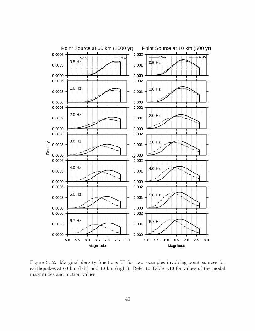
0.0000
0.0003
0.0006
0.0000
0.0003
0.0006
0.5 Hz
0.0000
0.0003
0.0006Vea
0.0000
0.0003
0.0006PSV
Point Source at 60 km (2500 yr)
0.0000
0.0003
0.0006
0.0000
0.0003
0.0006
1.0 Hz
0.0000
0.0003
0.0006
0.0000
0.0003
0.0006
2.0 Hz
0.0000
0.0003
0.0006
0.0000
0.0003
0.0006
3.0 Hz
0.0000
0.0003
0.0006
0.0000
0.0003
0.0006
4.0 Hz
Den
sity
0.0000
0.0003
0.0006
0.0000
0.0003
0.0006
5.0 Hz
0.0000
0.0003
0.0006
5.0 5.5 6.0 6.5 7.0 7.5 8.0
Magnitude
0.0000
0.0003
0.0006
5.0 5.5 6.0 6.5 7.0 7.5 8.0
Magnitude
6.7 Hz
0.000
0.001
0.002
0.000
0.001
0.002
0.5 Hz
0.000
0.001
0.002Vea
0.000
0.001
0.002PSV
Point Source at 10 km (500 yr)
0.000
0.001
0.002
0.000
0.001
0.002
1.0 Hz
0.000
0.001
0.002
0.000
0.001
0.002
2.0 Hz
0.000
0.001
0.002
0.000
0.001
0.002
3.0 Hz
0.000
0.001
0.002
0.000
0.001
0.002
4.0 Hz
¥
0.000
0.001
0.002
0.000
0.001
0.002
5.0 Hz
0.000
0.001
0.002
5.0 5.5 6.0 6.5 7.0 7.5 8.0
Magnitude
0.000
0.001
0.002
5.0 5.5 6.0 6.5 7.0 7.5 8.0
Magnitude
6.7 Hz
Figure 3.12: Marginal density functions U’ for two examples involving point sources forearthquakes at 60 km (left) and 10 km (right). Refer to Table 3.10 for values of the modalmagnitudes and motion values.
40

020
4060
Distance (Km) 5.05.5
6.06.5
7.07.5
Magnitude0.0
002
0.0
004
Densi
ty
0.0
002
0.0
004
Densi
ty 0.5 Hz
PSVContribution to Hazard: 500 yr Return Period
7.4
6.5
9:91
020
4060
Distance (Km) 5.05.5
6.06.5
7.07.5
Magnitude
0.0
002
0.0
004
Densi
ty
0.0
002
0.0
004
Densi
ty 1 Hz
7.2
6.4
17:83
020
4060
Distance (Km) 5.05.5
6.06.5
7.07.5
Magnitude
0.0
002
0.0
004
Densi
ty
0.0
002
0.0
004
Densi
ty 2 Hz
6.9
5.9
31:69
020
4060
Distance (Km) 5.05.5
6.06.5
7.07.5
Magnitude
0.0
002
0.0
004
Densi
ty
0.0
002
0.0
004
Densi
ty 3 Hz6.5
5.8
41:59
020
4060
Distance (Km) 5.05.5
6.06.5
7.07.5
Magnitude
0.0
002
0.0
004
Densi
ty
0.0
002
0.0
004
Densi
ty 6.7 Hz6.4
5.9
49:51
020
4060
Distance (Km) 5.05.5
6.06.5
7.07.5
Magnitude
0.0
002
0.0
004
0.0
002
0.0
004
0.5 Hz
Vea 7.4
6.5
6:94
020
4060
Distance (Km) 5.05.5
6.06.5
7.07.5
Magnitude
0.0
002
0.0
004
0.0
002
0.0
004
1 Hz
7.4
6.5
11:89
020
4060
Distance (Km) 5.05.5
6.06.5
7.07.5
Magnitude
0.0
002
0.0
004
0.0
002
0.0
004
2 Hz
7.1
6.3
21:79
020
4060
Distance (Km) 5.05.5
6.06.5
7.07.5
Magnitude
0.0
002
0.0
004
0.0
002
0.0
004
3 Hz
6.9
6.2
28:72
020
4060
Distance (Km) 5.05.5
6.06.5
7.07.5
Magnitude
0.0
002
0.0
004
0.0
002
0.0
004
6.7 Hz
6.9
6.2
31:69
Figure 3.13: Marginal density functions U’ for the example calculation in the text. Themodal magnitudes are indicated for each source, as are the relative contributions, in percentof the total hazard, of each source. The calculations are for a 500 year return period, andcombined A and B site class. Refer to Table 3.11 for values of the marginal and joint modalevents.
41

42
Table 3.1
Strong Motion Recordings Used in Regression Analysis
Earthquake Site Name Site Number* Az1 Az2 Dist (km) Lat. N Lon. W Class
Imperial Valley El Centro #9 (ct 117) 180 270 12.0 32.795 115.549 cMay 19, 1940M=7.0
Kern County Taft Lincoln sch (ct 95) 21 111 42.0 35.150 119.450 bJuly 21, 1952 Santa Barbara CH (ct 283) 42 132 85.0 34.424 119.701 bM=7.4 Cal Tech Athena. (ct 475) 180 270 109.0 34.139 118.121 b
Hollywood St. Bld. (ct 135) 180 90 107.0 34.083 118.333 c
Daly City Golden Gate Park (ct 077) 10 100 8.0 37.667 122.483 aMar. 22, 1957M=5.3
Parkfield Cholame Shandon #2 (ct 13) 65 --- 6.6 35.731 120.286 cJune 28, 1966 Cholame Shandon #5 (ct 14) 355 85 9.3 35.700 120.328 cM=6.1 Cholame Shandon #8 (ct 15) 50 320 13.0 35.671 120.360 c
Cholame Shandon #12 (ct 16) 50 320 17.3 35.636 120.403 bCholame Shandon Tmblor #2 (ct 97) 295 205 16.1 35.752 120.264 b
Borrego Mtn. El Centro Array #9 (ct 117) 90 270 45.0 32.794 115.54 cApril 9, 1968M=6.6
San Fernando Caltech Athenaeum (ct 475) 0 90 25.7 34.139 118.121 bFeb. 9, 1971 Lake Hughes Sta. 4 (ct 126) 111 201 19.6 34.642 118.480 cM=6.6 Lake Hughes Sta. 12 (ct 128) 21 249 17.0 34.572 118.560 b
Wrightwood (ct 290) 25 115 60.7 34.361 117.633 b
Sitka Sitka magnetic observatory (2714) 180 90 45.0 57.060 135.320 aJuly 30, 1972M=7.7
Managua ESSO Refinery ---- 180 90 5.0 12.145 86.322 cDec. 23, 1972M=6.2
Hollister San Juan Buatista --- 237 33 10.0 36.860 121.540 cNov. 28, 1974 Hollister City Hall annex (usgs 1575) 181 271 19.0 36.851 121.402 cM=5.2 Gilroy -Gavilan College (cdmg 47379) 247 157 22.0 36.973 121.572 b
St. Elias Icy Bay, Gulf Timber Co. (2734) 180 90 25.4 59.968 141.643 bFeb. 28, 1979M=7.6
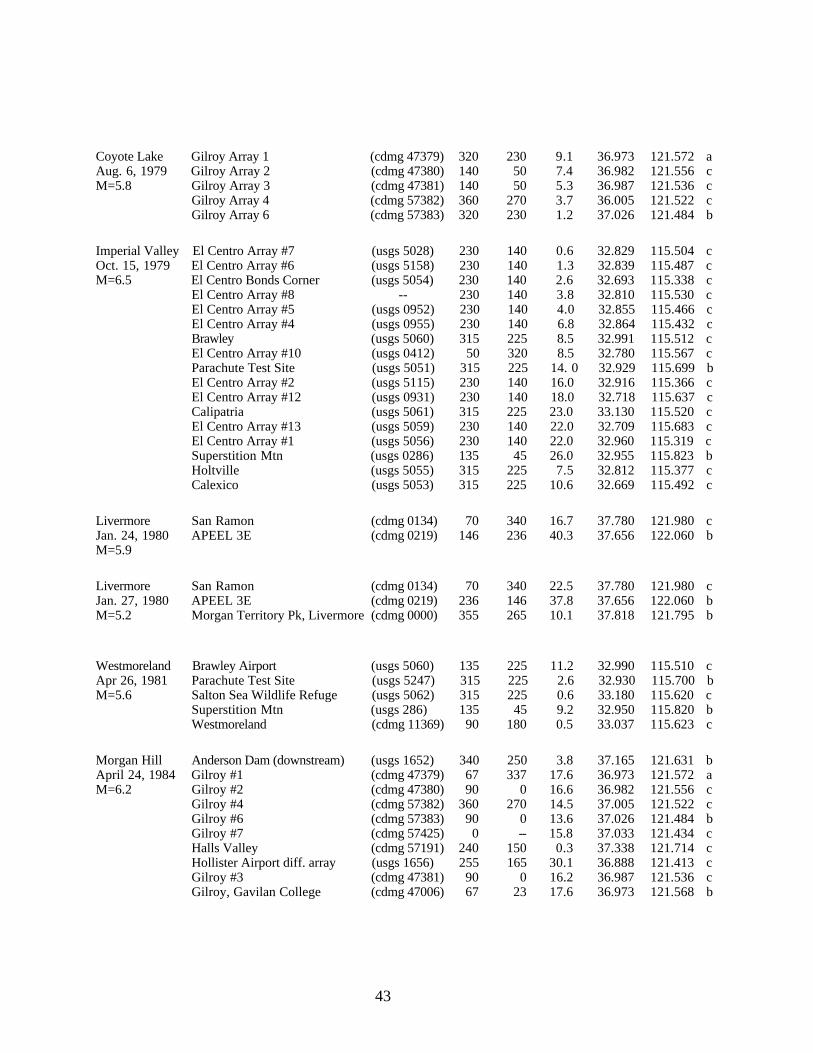
43
Coyote Lake Gilroy Array 1 (cdmg 47379) 320 230 9.1 36.973 121.572 aAug. 6, 1979 Gilroy Array 2 (cdmg 47380) 140 50 7.4 36.982 121.556 cM=5.8 Gilroy Array 3 (cdmg 47381) 140 50 5.3 36.987 121.536 c
Gilroy Array 4 (cdmg 57382) 360 270 3.7 36.005 121.522 cGilroy Array 6 (cdmg 57383) 320 230 1.2 37.026 121.484 b
Imperial Valley El Centro Array #7 (usgs 5028) 230 140 0.6 32.829 115.504 cOct. 15, 1979 El Centro Array #6 (usgs 5158) 230 140 1.3 32.839 115.487 cM=6.5 El Centro Bonds Corner (usgs 5054) 230 140 2.6 32.693 115.338 c
El Centro Array #8 -- 230 140 3.8 32.810 115.530 cEl Centro Array #5 (usgs 0952) 230 140 4.0 32.855 115.466 cEl Centro Array #4 (usgs 0955) 230 140 6.8 32.864 115.432 cBrawley (usgs 5060) 315 225 8.5 32.991 115.512 cEl Centro Array #10 (usgs 0412) 50 320 8.5 32.780 115.567 cParachute Test Site (usgs 5051) 315 225 14. 0 32.929 115.699 bEl Centro Array #2 (usgs 5115) 230 140 16.0 32.916 115.366 cEl Centro Array #12 (usgs 0931) 230 140 18.0 32.718 115.637 cCalipatria (usgs 5061) 315 225 23.0 33.130 115.520 cEl Centro Array #13 (usgs 5059) 230 140 22.0 32.709 115.683 cEl Centro Array #1 (usgs 5056) 230 140 22.0 32.960 115.319 cSuperstition Mtn (usgs 0286) 135 45 26.0 32.955 115.823 bHoltville (usgs 5055) 315 225 7.5 32.812 115.377 cCalexico (usgs 5053) 315 225 10.6 32.669 115.492 c
Livermore San Ramon (cdmg 0134) 70 340 16.7 37.780 121.980 cJan. 24, 1980 APEEL 3E (cdmg 0219) 146 236 40.3 37.656 122.060 bM=5.9
Livermore San Ramon (cdmg 0134) 70 340 22.5 37.780 121.980 cJan. 27, 1980 APEEL 3E (cdmg 0219) 236 146 37.8 37.656 122.060 bM=5.2 Morgan Territory Pk, Livermore (cdmg 0000) 355 265 10.1 37.818 121.795 b
Westmoreland Brawley Airport (usgs 5060) 135 225 11.2 32.990 115.510 cApr 26, 1981 Parachute Test Site (usgs 5247) 315 225 2.6 32.930 115.700 bM=5.6 Salton Sea Wildlife Refuge (usgs 5062) 315 225 0.6 33.180 115.620 c
Superstition Mtn (usgs 286) 135 45 9.2 32.950 115.820 bWestmoreland (cdmg 11369) 90 180 0.5 33.037 115.623 c
Morgan Hill Anderson Dam (downstream) (usgs 1652) 340 250 3.8 37.165 121.631 bApril 24, 1984 Gilroy #1 (cdmg 47379) 67 337 17.6 36.973 121.572 aM=6.2 Gilroy #2 (cdmg 47380) 90 0 16.6 36.982 121.556 c
Gilroy #4 (cdmg 57382) 360 270 14.5 37.005 121.522 cGilroy #6 (cdmg 57383) 90 0 13.6 37.026 121.484 bGilroy #7 (cdmg 57425) 0 -- 15.8 37.033 121.434 cHalls Valley (cdmg 57191) 240 150 0.3 37.338 121.714 cHollister Airport diff. array (usgs 1656) 255 165 30.1 36.888 121.413 cGilroy #3 (cdmg 47381) 90 0 16.2 36.987 121.536 cGilroy, Gavilan College (cdmg 47006) 67 23 17.6 36.973 121.568 b
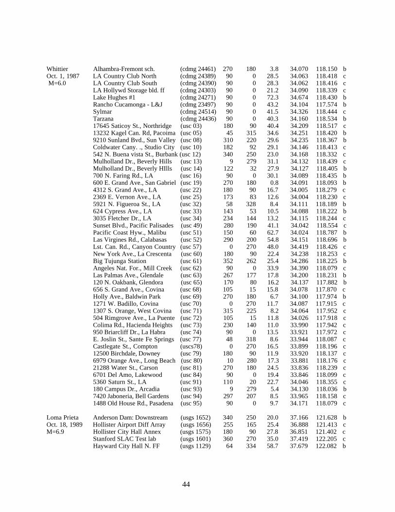
44
Whittier Alhambra-Fremont sch. (cdmg 24461) 270 180 3.8 34.070 118.150 bOct. 1, 1987 LA Country Club North (cdmg 24389) 90 0 28.5 34.063 118.418 c M=6.0 LA Country Club South (cdmg 24390) 90 0 28.3 34.062 118.416 c
LA Hollywd Storage bld. ff (cdmg 24303) 90 0 21.2 34.090 118.339 c Lake Hughes #1 (cdmg 24271) 90 0 72.3 34.674 118.430 b
Rancho Cucamonga - L&J (cdmg 23497) 90 0 43.2 34.104 117.574 bSylmar (cdmg 24514) 90 0 41.5 34.326 118.444 cTarzana (cdmg 24436) 90 0 40.3 34.160 118.534 b17645 Saticoy St., Northridge (usc 03) 180 90 40.4 34.209 118.517 c13232 Kagel Can. Rd, Pacoima (usc 05) 45 315 34.6 34.251 118.420 b9210 Sunland Bvd., Sun Valley (usc 08) 310 220 29.6 34.235 118.367 bColdwater Cany. ., Studio City (usc 10) 182 92 29.1 34.146 118.413 c542 N. Buena vista St., Burbank (usc 12) 340 250 23.0 34.168 118.332 cMulholland Dr., Beverly Hills (usc 13) 9 279 31.1 34.132 118.439 cMulholland Dr., Beverly HIlls (usc 14) 122 32 27.9 34.127 118.405 b700 N. Faring Rd., LA (usc 16) 90 0 30.1 34.089 118.435 b600 E. Grand Ave., San Gabriel (usc 19) 270 180 0.8 34.091 118.093 b4312 S. Grand Ave., LA (usc 22) 180 90 16.7 34.005 118.279 c2369 E. Vernon Ave., LA (usc 25) 173 83 12.6 34.004 118.230 c5921 N. Figueroa St., LA (usc 32) 58 328 8.4 34.111 118.189 b624 Cypress Ave., LA (usc 33) 143 53 10.5 34.088 118.222 b3035 Fletcher Dr., LA (usc 34) 234 144 13.2 34.115 118.244 cSunset Blvd., Pacific Palisades (usc 49) 280 190 41.1 34.042 118.554 cPacific Coast Hyw., Malibu (usc 51) 150 60 62.7 34.024 118.787 bLas Virgines Rd., Calabasas (usc 52) 290 200 54.8 34.151 118.696 bLst. Can. Rd., Canyon Country (usc 57) 0 270 48.0 34.419 118.426 cNew York Ave., La Crescenta (usc 60) 180 90 22.4 34.238 118.253 cBig Tujunga Station (usc 61) 352 262 25.4 34.286 118.225 bAngeles Nat. For., Mill Creek (usc 62) 90 0 33.9 34.390 118.079 cLas Palmas Ave., Glendale (usc 63) 267 177 17.8 34.200 118.231 b120 N. Oakbank, Glendora (usc 65) 170 80 16.2 34.137 117.882 b656 S. Grand Ave., Covina (usc 68) 105 15 15.8 34.078 117.870 cHolly Ave., Baldwin Park (usc 69) 270 180 6.7 34.100 117.974 b1271 W. Badillo, Covina (usc 70) 0 270 11.7 34.087 117.915 c1307 S. Orange, West Covina (usc 71) 315 225 8.2 34.064 117.952 c504 Rimgrove Ave., La Puente (usc 72) 105 15 11.8 34.026 117.918 cColima Rd., Hacienda Heights (usc 73) 230 140 11.0 33.990 117.942 c950 Briarcliff Dr., La Habra (usc 74) 90 0 13.5 33.921 117.972 cE. Joslin St., Sante Fe Springs (usc 77) 48 318 8.6 33.944 118.087 cCastlegate St., Compton (uscs78) 0 270 16.5 33.899 118.196 c12500 Birchdale, Downey (usc 79) 180 90 11.9 33.920 118.137 c6979 Orange Ave., Long Beach (usc 80) 10 280 17.3 33.881 118.176 c21288 Water St., Carson (usc 81) 270 180 24.5 33.836 118.239 c6701 Del Amo, Lakewood (usc 84) 90 0 19.4 33.846 118.099 c5360 Saturn St., LA (usc 91) 110 20 22.7 34.046 118.355 c180 Campus Dr., Arcadia (usc 93) 9 279 5.4 34.130 118.036 b7420 Jaboneria, Bell Gardens (usc 94) 297 207 8.5 33.965 118.158 c1488 Old House Rd., Pasadena (usc 95) 90 0 9.7 34.171 118.079 c
Loma Prieta Anderson Dam: Downstream (usgs 1652) 340 250 20.0 37.166 121.628 bOct. 18, 1989 Hollister Airport Diff Array (usgs 1656) 255 165 25.4 36.888 121.413 cM=6.9 Hollister City Hall Annex (usgs 1575) 180 90 27.8 36.851 121.402 c Stanford SLAC Test lab (usgs 1601) 360 270 35.0 37.419 122.205 c
Hayward City Hall N. FF (usgs 1129) 64 334 58.7 37.679 122.082 b

45
APEEL station 9 (usgs 1161) 227 137 46.4 37.478 122.321 bBear Valley sta. 5 (usgs 1474) 310 220 53.7 36.673 121.195 bBear Valley sta. 10 (usgs 1479) 310 220 67.3 36.532 121.143 c
Bear Valley sta. 12 (usgs 1481) 310 220 50.9 36.658 121.249 cCalaveras Res. South gnd. (usgs 1687) 180 90 36.1 37.452 121.807 bCherry Flat Reservoir (usgs 1696) 360 270 32.5 37.396 121.756 aDublin Fire Station (usgs 1689) 360 270 61.6 37.709 121.932 c
Hollister Sago Vault (usgs 1032) 360 270 29.9 36.765 121.446 a Sunol Fire Station (usgs 1688) 180 90 49.9 37.597 121.880 b Agnew (cdmg 57066) 90 0 27.0 37.397 121.952 c Gilroy # 1 (cdmg 47379) 90 0 10.5 36.973 121.572 a
Monterey city hall (cdmg 47377) 90 0 42.7 36.597 121.897 aSan Fran. Sierra Point (cdmg 58539) 205 115 67.6 37.674 122.388 aCorralitos (cdmg 57007) 90 0 0.1 37.046 121.803 b
Gilroy #1 Gavilan College (cdmg 47006) 67 337 10.9 36.973 121.568 bSaratoga (cdmg 58065) 90 0 11.7 37.255 122.031 b
Santa Cruz (cdmg 58135) 90 0 12.5 37.001 122.060 bSan Jose: Santa Teresa Hills (cdmg 57563) 225 315 13.2 37.210 121.803 bGilroy #6 (cdmg 57383) 90 0 19.9 37.026 121.484 b
SAGO south (cdmg 47189) 351 261 34.1 36.753 121.396 bWoodside (cdmg 58127) 90 0 38.7 37.429 122.258 bHayward BART FF (cdmg 58498) 310 220 57.7 37.670 122.086 bCapitola (cdmg 47125) 90 0 8.6 36.974 121.952 cGilroy #2 (cdmg 47380) 90 0 12.1 36.982 121.556 cGilroy #3 (cdmg 47381) 90 0 14.0 36.987 121.536 cGilroy #4 (cdmg 57382) 90 0 15.8 37.005 121.522 cGilroy #7 (cdmg 57425) 90 0 24.3 37.033 121.434 cHalls Valley (cdmg 57191) 90 0 29.3 37.338 121.714 c
Salinas (cdmg 47179) 250 160 31.4 36.671 121.642 c Fremont (cdmg 57064) 90 0 42.4 37.535 121.929 c
San Fran. Airport (cdmg 58223) 90 0 63.2 37.622 122.398 c
Sierra Madre 17645 Saticoy St., Northridge (usc 03) 180 90 44.0 34.209 118.517 cJune 28, 1991 600 E. Grand Ave., San Gabriel (usc 19) 270 180 17.7 34.091 118.093 bM=5.6 3035 Fletcher Dr., LA (usc 34) 234 144 23.8 34.115 118.244 c
Canoga Park (usc 53) 196 106 52.1 34.212 118.606 cLst. Can. Rd., Canyon Country (usc 57) 0 270 39.9 34.419 118.426 cNew York Ave., La Crescenta (usc 60) 180 90 19.6 34.238 118.254 cBig Tujunga Station (usc 61) 352 262 17.3 34.286 118.225 bLas Palmas Ave., Glendale (usc 63) 267 177 18.4 34.200 118.231 b120 N. Oakbank, Glendora (usc 65) 170 80 14.8 34.137 117.883 b11338 Fariview Ave., El Monte (usc 66) 185 95 16.7 34.093 118.019 c237 Mel Canyon Rd., Duarte (usc 67) 180 90 11.6 34.150 117.939 bHolly Ave., Baldwin Park (usc 69) 270 180 16.1 34.100 117.974 b1271 W. Badillo, Covina (usc 70) 0 270 18.9 34.087 117.915 c1307 S. Orange, West Covina (usc 71) 315 225 20.4 34.064 117.952 cE. Joslin St., Sante Fe Springs (usc 77) 48 318 33.5 33.944 118.087 c180 Campus Dr., Arcadia (usc 93) 9 279 12.6 34.130 118.036 b7420 Jaboneria, Bell Gardens (usc 94) 310 220 32.8 33.965 118.158 c855 Arcadia Ave., Arcadia (usc 99) 262 172 13.1 34.127 118.059 c
Petrolia Ferndale Fire Sta (usgs 1023) 360 270 10.0 40.576 124.262 cApril 25, 1992 Loleta Fire Sta (usgs 1586) 360 270 17.6 40.644 124.219 bM=7.1 Centerville Beach (usgs 1585) 360 270 9.8 40.563 124.348 b
College of Redwood (usgs 1582) 360 270 23.9 40.699 124.200 b

46
South Bay school (usgs 1581) 360 270 27.8 40.735 124.207 cFortuna Fire Sta (usgs 1583) 360 270 14.6 40.599 124.154 bBunker Hill FAA (usgs 1584) 360 270 1.9 40.498 124.294 a
Landers Twentynine Palms (cdmg 22161) 90 0 41.9 34.021 116.009 aJune 28, 1992 Silent Valley (cdmg 12206) 90 0 51.3 33.851 116.852 aM=7.3 Joshua Tree (cdmg 22170) 90 0 11.3 34.131 116.314 b
Desert hot Springs (cdmg 12149) 90 0 22.5 33.962 116.509 b Barstow (cdmg 23559) 90 0 37.7 34.887 117.047 b Fort irwin (cdmg 24577) 90 0 65.0 35.268 116.684 b Yermo (cdmg 22074) 90 0 26.3 34.903 116.823 c Palm Springs (cdmg 12025) 90 0 36.7 33.829 116.501 c
Indio (cdmg 12026) 90 0 54.9 33.717 116.156 cAmboy (cdmg 21081) 90 0 68.3 34.560 115.743 aBaker (cdmg 32075) 140 50 88.3 35.272 116.066 bBoron (cdmg 33083) 90 0 92.4 35.002 117.650 bHemet (cdmg 12331) 90 0 69.1 33.729 116.979 cPuerta La Cruz (cdmg 12168) 90 0 95.0 33.324 116.683 bRiverside Airport (cdmg 13123) 270 180 96.2 33.951 117.446 bSan Bernadino E & H (cdmg 23542) 90 180 79.9 34.065 117.292 cN. Palm Sprngs fs (usgs 5295) 180 90 27.7 33.924 116.543 bWhitewater Canyon (usgs 5072) 270 180 27.6 33.989 116.655 aMorongo Valley (usgs 5071) 135 45 17.7 34.048 116.577 bForest Falls (usgs 5075) 300 210 45.4 34.088 116.919 bIndio Jackson rd (usgs 5294) 180 90 49.6 33.747 116.214 cFun Valley (usgs 5069) 135 45 25.8 33.930 116.390 bThousand Palms (usgs 5068) 135 45 37.7 33.820 116.400 cEuclid st., Fountain Valley (usc 02) 22 292 144.2 33.719 117.938 cRoscoe Blvd., Sun Valley (usc 06) 90 0 162.8 34.221 118.421 bBuena Vista St., Burbank (usc 12) 340 250 157.2 34.168 118.332 c924 W. 70th St., LA (usc 23) 0 270 163.0 33.976 118.289 c5921 N. Figueroa St., LA (usc 32) 58 328 147.8 34.111 118.189 b3036 Fletcher Dr., LA (usc 34) 234 144 152.2 34.115 118.244 cN. Las Virginies Rd., Calabasas (usc 52) 290 200 189.4 34.151 118.697 bMt. Gleason Ave., Sunland (usc 58) 260 170 150.8 34.269 118.303 bBig Tujunga Station (usc 61) 352 262 143.4 34.286 118.225 bLas Palmas Ave., Glendale (usc 63) 267 177 147.3 34.200 118.231 c120 N. Oakbank, Glendora (usc 65) 170 80 121.5 34.137 117.882 b
Colima Rd., Hacienda Heights (usc 73) 230 140 135.1 33.990 117.942 c180 Campus Dr., Arcadia (usc 93) 9 279 134.3 34.130 118.036 b
Big Bear Big Bear Lake - civic center (cdmg 22561) 270 360 10.2 34.238 116.935 bJune 28, 1992 San Bernadino E & H (cdmg 23542) 90 180 39.7 34.065 117.292 cM=6.2 N.Palm Springs FS (usgs 5295) 180 90 36.2 33.924 116.543 b
San Bernadino, Highland FS (usgs 5161) 315 225 31.3 34.136 117.213 cMorongo Valley (usgs 5071) 135 45 24.6 34.048 116.577 bFun Valley (usgs 5069) 135 45 45.7 33.930 116.390 bEuclid st., Fountain Valley (usc 02) 22 292 109.2 33.719 117.938 c120 N. Oakbank, Glendora (usc 65) 170 80 93.0 34.137 117.882 b656 S. Grand Ave., Covina (usc 68) 74 344 92.4 34.078 117.871 c1271 W. Badillo, Covina (usc 70) 0 270 96.3 34.087 117.915 c504 Rimgrove Ave., La Puente (usc 72) 105 15 97.4 34.026 117.918 cColima Rd., Hacienda Heights (usc 73) 230 140 100.2 33.990 117.942 cE. Joslin St., Santa Fe Springs (usc 77) 120 30 114.3 33.944 118.087 c200 S. Flower Ave., Brea (usc 87) 20 290 97.9 33.916 117.896 c

47
17852 Serrano Ave., Villa Park (usc 90) 0 270 94.4 33.821 117.818 b180 Campus Dr., Arcadia (usc 93) 9 279 107.2 34.130 118.036 b7420 Jaboneria, Bell Gardens (usc 94) 310 220 120.3 33.965 118.158 c
Northridge Alhambra - Fremont Sch. (cdmg 24461) 90 360 36.2 34.070 118.150 bJan. 17, 1994 Castaic Old Ridge Rt. (cdmg 24278) 90 360 20.8 34.564 118.642 bM=6.7 Century City - LACC north (cdmg 24389) 90 360 17.4 34.063 118.418 c Lake Hughes #1 fs (cdmg 24271) 90 0 36.1 34.674 118.430 b
Lake Hughes 4 (cdmg 24469) 90 0 31.9 34.650 118.478 cLake Hughes #4b (cdmg 24523) 90 0 32.0 34.650 118.477 c
Lake Hughes #9 (cdmg 24272) 90 360 25.6 34.608 118.558 aLake Hughes #12a (cdmg 24607) 90 180 21.5 34.571 118.560 b
Littlerock - Brainard Canyon (cdmg 23595) 90 180 46.7 34.486 117.980 a Long Beach - City Hall grounds (cdmg 14560) 90 360 56.0 33.768 118.196 c
LA - Hollywood stor.blg. (cdmg 24303) 90 360 20.0 34.090 118.339 c Mt. Baldy - Elem. School (cdmg 23572) 90 180 72.2 34.233 117.661 a Mt. Wilson (cdmg 24399) 90 360 36.5 34.224 118.057 a Phelan - Wilson Ranch Rd. (cdmg 23597) 90 180 86.4 34.467 117.520 b Port Hueneme - Naval Lab. (cdmg 25281) 180 90 49.8 34.145 119.206 c Rancho Cucamonga-Deer Can. (cdmg 23598) 90 180 80.8 34.169 117.579 a Rancho Cucamonga - L&J FF (cdmg 23497) 90 0 82.9 34.104 117.574 b
Rancho Palos Verdes (cdmg 14404) 90 0 50.8 33.746 118.396 aRiverside airport (cdmg 13123) 270 180 99.8 33.951 117.446 b
San Bernardino - E & H (cdmg 23542) 90 180 109.2 34.065 117.292 c Sylmar - County Hospital PL (cdmg 24514) 90 360 1.7 34.326 118.444 c Tarzana Cedar Hill Nur. A (cdmg 24436) 90 360 3.4 34.160 118.534 b Wrightwood - Jackson Flat (cdmg 23590) 90 180 65.2 34.381 117.737 a
Wrightwood - Nielson Ranch (cdmg 23573) 90 180 82.4 34.314 117.545 bWrightwood - Swarthout Valley (cdmg 23574) 90 180 72.3 34.369 117.658 b17645 Saticoy St. Northridge (usc 03) 180 90 0.2 34.209 118.517 c12001 Chalon Rd. LA (usc 15) 70 160 12.4 34.086 118.481 b700 N. Faring Rd, LA (usc 16) 0 90 14.1 34.089 118.435 b
8510 Wonderland Ave, LA (usc 17) 185 95 15.4 34.114 118.380 aWilloughby Ave. Hollywood (usc 18) 180 90 18.3 34.088 118.365 b600 E. Grand Av., San Gabriel (usc 19) 180 270 39.4 34.091 118.093 b2628 W. 15th. St., LA (usc 20) 180 90 26.1 34.045 118.298 c4312 S. Grand Ave, LA (usc 22) 180 90 30.4 34.005 118.279 c2369 E. Vernon Ave, LA (usc 25) 180 90 33.8 34.004 118.230 c624 Cypress Ave., LA (usc 33) 53 143 29.4 34.088 118.222 b3036 Fletcher Dr., LA (usc 34) 144 234 26.2 34.115 118.244 c23536 Catskill Ave., Carson (usc 40) 180 90 48.3 33.812 118.270 cRancho Palos Verdes (usc 44) 5 95 53.1 33.740 118.335 c14801 Osage Ave, Lawndale (usc 45) 182 92 36.7 33.897 118.346 cManhattan Beach (usc 46) 0 90 36.1 33.886 118.389 cCanoga Park (usc 53) 196 106 1.6 34.212 118.606 c3960 Centinela St., LA (usc 54) 155 245 22.9 34.001 118.431 cCanyon Country (usc 57) 0 270 11.4 34.419 118.426 c1250 Howard rd., Burbank (usc 59) 330 60 16.5 34.204 118.302 aNew York Ave., La Crescenta (usc 60) 180 90 18.8 34.238 118.254 cBig Tujunga Station (usc 61) 352 262 19.9 34.286 118.225 b3320 Las Palmas Ave., Glendale (usc 63) 177 267 22.3 34.200 118.231 b120 N. Oakbank, Glendora (usc 65) 80 170 54.8 34.137 117.882 bFairview Ave., El Monte (usc 66) 185 95 45.2 34.093 118.019 c237 Mel Canyon Rd., Duarte (usc 67) 90 180 49.3 34.150 117.939 b656 S. Grand Ave., Covina (usc 68) 344 74 58.1 34.078 117.871 c

48
3699 Holly Ave., Baldwin Park (usc 69) 180 270 48.5 34.100 117.974 b1271 W. Badillo, Covina (usc 70) 360 270 54.0 34.087 117.915 c
S. Orange Ave., West Covina (usc 71) 315 225 52.1 34.064 117.952 c504 Rimgrove Ave., La Puente (usc 72) 15 105 57.0 34.026 117.918 cColima Rd., Hacienda Heights (usc 73) 140 230 57.3 33.990 117.942 c
6302 S. Alta Dr. Whittier (usc 75) 0 90 48.9 34.015 118.029 bE. Joslin St., Santa Fe Springs (usc 77) 30 120 48.3 33.944 118.087 c
14637 Castlegate st., Compton (usc 78) 360 270 44.2 33.899 118.196 c21288 Water St., Carson (usc 81) 180 270 47.4 33.836 118.240 cTerminal Island (usc 82) 330 240 55.8 33.736 118.269 cHuntington Beach (usc 83) 290 200 67.9 33.727 118.044 cDel Amo Blvd., Lakewood (usc 84) 0 90 54.6 33.846 118.099 c6861 Santa Rita, Garden Grove (usc 85) 360 270 64.7 33.790 118.012 cLa Palma ave., Buena Park (usc 86) 180 90 60.0 33.847 118.018 c200 S. Flower Ave., Brea (usc 87) 20 290 64.9 33.916 117.896 c2000 W. Ball Rd., Anaheim (usc 88) 0 90 66.9 33.817 117.951 c
5360 Saturn St., LA (usc 91) 20 110 22.3 34.046 118.355 c180 Campus Dr., Arcadia (usc 93) 9 279 41.9 34.130 118.036 b7420 Jaboneria, Bell Gardens (usc 94) 310 220 41.7 33.965 118.158 c3620 S. Vermont Ave., LA (usc 96) 0 90 28.1 34.022 118.293 c855 Arcadia Ave., Arcadia (usc 99) 172 262 40.1 34.127 118.059 cGriffith Observatory (usgs 141) 360 270 21.5 34.118 118.299 aLittlerock Post Office (usgs 5030) 300 210 47.6 34.520 117.990 bPardo Dam Downstream (usgs 969) 90 360 86.7 33.890 117.641 cLong Beach VA Hospital (usgs 5106) 360 270 59.2 33.778 118.118 b
NSMP Pasadena Lab. (usgs 5296) 360 270 34.1 34.136 118.127 b
* ct: California Institute of Technology Civil Engineering Dept.usc: University of Southern California Civil Engineering Dept.cdmg: California Division of Mines and Geology Strong Motion Instrumentation Programusgs: U. S. Geological Survey National Strong Motion Program

49
Table 3.2
NEHRP* Site Class
Site Class Range of Shear Velocities
A >1500 m/s
B 760 m/s to 1500 m/s
C 360 m/s to 760 m/s
D 180 m/s to 360 m/s
E < 180 m/s
* BSSC (1994)

50
Table 3.3
Regression Coefficients for Peak Ground Acceleration and Velocity,
Randomly Oriented Horizontal Component
PGA
a b c d h e f σ3.098 0.3065 -0.07570 -0.8795 6.910 0.1452 0.1893 0.2124
PGV
a b c d h e f σ1.747 0.4481 -0.03248 -0.8075 3.992 0.1862 0.3009 0.2470
Regression coefficients refer to Equation 3.7, for the base 10 logarithm of motion, PGA in units of
cm/sec2 and PGV in units of cm/sec.

51
TABLE 3.4 PSV 2% Damping
Regression coefficients refer to Equation 3.7, for the base 10 logarithm of motion, randomlyoriented horizontal component (cm/sec)
Freq. (Hz) a b c d h e f σ 0.500 1.581 0.638 -0.037 -0.695 2.773 0.267 0.452 0.326 0.526 1.588 0.631 -0.061 -0.693 3.123 0.293 0.474 0.327 0.556 1.614 0.627 -0.070 -0.694 3.427 0.296 0.471 0.326 0.588 1.637 0.607 -0.060 -0.693 3.512 0.290 0.468 0.319 0.625 1.700 0.599 -0.059 -0.731 3.664 0.291 0.472 0.311 0.667 1.715 0.586 -0.033 -0.748 3.476 0.303 0.476 0.302 0.714 1.709 0.569 -0.039 -0.717 2.966 0.282 0.450 0.302 0.769 1.745 0.541 -0.047 -0.708 2.945 0.260 0.429 0.306 0.833 1.814 0.544 -0.070 -0.703 3.340 0.216 0.388 0.290 0.909 1.774 0.524 -0.079 -0.658 3.163 0.213 0.391 0.288 1.000 1.844 0.501 -0.045 -0.700 3.723 0.219 0.372 0.277 1.053 1.871 0.496 -0.039 -0.724 3.383 0.223 0.368 0.282 1.111 1.891 0.500 -0.043 -0.738 3.201 0.218 0.368 0.287 1.176 1.875 0.497 -0.047 -0.733 2.881 0.226 0.376 0.284 1.250 1.866 0.493 -0.060 -0.716 2.674 0.202 0.361 0.290 1.333 1.915 0.494 -0.074 -0.753 2.850 0.224 0.368 0.292 1.429 1.974 0.505 -0.082 -0.796 3.304 0.221 0.375 0.294 1.538 2.013 0.463 -0.057 -0.798 3.472 0.183 0.343 0.291 1.667 2.023 0.465 -0.087 -0.795 3.717 0.197 0.335 0.292 1.818 1.973 0.406 -0.065 -0.741 3.512 0.195 0.340 0.279 2.000 2.001 0.390 -0.057 -0.768 4.388 0.224 0.352 0.269 2.083 1.985 0.380 -0.053 -0.757 4.137 0.219 0.343 0.271 2.174 1.958 0.364 -0.051 -0.733 3.963 0.213 0.337 0.274 2.273 1.986 0.368 -0.053 -0.742 3.952 0.188 0.307 0.278 2.381 2.023 0.367 -0.069 -0.761 4.186 0.187 0.287 0.274 2.500 2.045 0.333 -0.043 -0.777 4.538 0.177 0.283 0.268 2.632 2.099 0.321 -0.043 -0.804 5.036 0.158 0.256 0.262 2.778 2.096 0.338 -0.063 -0.814 5.274 0.182 0.266 0.266 2.941 2.122 0.341 -0.080 -0.814 5.361 0.165 0.235 0.262 3.125 2.101 0.349 -0.090 -0.809 5.413 0.166 0.235 0.262 3.333 2.083 0.358 -0.116 -0.796 5.859 0.171 0.237 0.255 3.571 2.204 0.370 -0.131 -0.867 7.914 0.153 0.198 0.246 3.846 2.160 0.359 -0.123 -0.858 8.085 0.154 0.186 0.243 4.167 2.219 0.362 -0.121 -0.906 8.782 0.143 0.170 0.243 4.545 2.193 0.350 -0.129 -0.895 9.549 0.151 0.165 0.238 5.000 2.325 0.370 -0.163 -0.962 11.380 0.117 0.116 0.238 5.263 2.271 0.363 -0.166 -0.953 10.400 0.125 0.130 0.238 5.556 2.275 0.335 -0.155 -0.975 10.590 0.132 0.130 0.241 5.882 2.200 0.318 -0.156 -0.953 10.870 0.155 0.145 0.243 6.250 2.313 0.303 -0.140 -1.029 12.470 0.130 0.126 0.241 6.667 2.314 0.310 -0.150 -1.052 12.850 0.123 0.121 0.239 7.143 2.325 0.301 -0.134 -1.111 12.850 0.147 0.139 0.243 7.692 2.265 0.299 -0.124 -1.098 12.920 0.124 0.117 0.240 8.333 2.185 0.308 -0.128 -1.085 11.860 0.098 0.101 0.234 9.091 2.096 0.252 -0.079 -1.092 11.400 0.112 0.113 0.25210.00 2.061 0.254 -0.090 -1.096 11.570 0.091 0.087 0.247

52
TABLE 3.5PSV 5% Damping
Regression coefficients refer to Equation 3.7, for the base 10 logarithm of motion, randomlyoriented horizontal component (cm/sec)
Freq. (Hz) a b c d h e f σ 0.500 1.547 0.627 -0.046 -0.729 2.929 0.275 0.449 0.316 0.526 1.563 0.621 -0.066 -0.724 3.145 0.279 0.451 0.318 0.556 1.572 0.609 -0.065 -0.722 3.302 0.287 0.456 0.315 0.588 1.593 0.597 -0.065 -0.722 3.400 0.288 0.459 0.310 0.625 1.634 0.588 -0.063 -0.744 3.543 0.294 0.464 0.304 0.667 1.648 0.575 -0.048 -0.755 3.390 0.300 0.463 0.299 0.714 1.654 0.554 -0.046 -0.733 3.005 0.276 0.433 0.297 0.769 1.713 0.542 -0.055 -0.739 3.121 0.243 0.404 0.297 0.833 1.767 0.530 -0.061 -0.739 3.401 0.211 0.380 0.285 0.909 1.750 0.516 -0.074 -0.706 3.302 0.204 0.374 0.283 1.000 1.789 0.490 -0.047 -0.730 3.561 0.216 0.368 0.277 1.053 1.822 0.489 -0.043 -0.753 3.420 0.213 0.360 0.279 1.111 1.834 0.487 -0.043 -0.765 3.182 0.211 0.361 0.283 1.176 1.830 0.486 -0.045 -0.771 2.983 0.222 0.371 0.284 1.250 1.830 0.481 -0.054 -0.768 2.914 0.217 0.368 0.285 1.333 1.869 0.480 -0.062 -0.796 3.087 0.225 0.370 0.287 1.429 1.904 0.482 -0.072 -0.812 3.367 0.214 0.363 0.292 1.538 1.939 0.454 -0.052 -0.823 3.503 0.189 0.344 0.288 1.667 1.930 0.442 -0.072 -0.810 3.562 0.200 0.341 0.286 1.818 1.923 0.406 -0.061 -0.792 3.850 0.204 0.342 0.277 2.000 1.914 0.376 -0.049 -0.787 4.116 0.217 0.350 0.270 2.083 1.898 0.362 -0.046 -0.774 3.955 0.214 0.344 0.271 2.174 1.885 0.350 -0.042 -0.759 3.942 0.204 0.332 0.271 2.273 1.894 0.344 -0.041 -0.761 3.999 0.191 0.315 0.272 2.381 1.929 0.344 -0.051 -0.779 4.208 0.181 0.296 0.270 2.500 1.964 0.329 -0.048 -0.799 4.545 0.173 0.283 0.264 2.632 1.972 0.315 -0.048 -0.807 4.767 0.171 0.278 0.262 2.778 1.981 0.324 -0.059 -0.818 4.948 0.179 0.274 0.264 2.941 1.998 0.322 -0.066 -0.826 5.236 0.178 0.262 0.260 3.125 1.997 0.335 -0.085 -0.824 5.409 0.177 0.249 0.256 3.333 1.998 0.340 -0.105 -0.824 5.854 0.177 0.240 0.248 3.571 2.060 0.344 -0.111 -0.865 7.022 0.164 0.211 0.242 3.846 2.082 0.346 -0.114 -0.885 7.589 0.156 0.187 0.237 4.167 2.090 0.347 -0.115 -0.906 8.303 0.157 0.188 0.236 4.545 2.101 0.341 -0.127 -0.915 9.229 0.152 0.175 0.232 5.000 2.181 0.350 -0.149 -0.962 10.670 0.132 0.138 0.230 5.263 2.153 0.345 -0.151 -0.964 10.270 0.139 0.144 0.229 5.556 2.146 0.334 -0.150 -0.976 10.260 0.139 0.143 0.230 5.882 2.102 0.319 -0.151 -0.967 10.450 0.148 0.149 0.232 6.250 2.115 0.301 -0.133 -0.990 10.790 0.136 0.137 0.229 6.667 2.108 0.300 -0.133 -1.010 11.050 0.130 0.130 0.230 7.143 2.121 0.297 -0.126 -1.053 11.670 0.141 0.146 0.228 7.692 2.057 0.285 -0.109 -1.047 11.570 0.138 0.144 0.225 8.333 1.986 0.284 -0.106 -1.033 10.850 0.114 0.123 0.224 9.091 1.915 0.254 -0.075 -1.044 10.540 0.120 0.135 0.23310.000 1.857 0.248 -0.071 -1.044 10.430 0.112 0.121 0.230

53
TABLE 3.6PSV 10% Damping
Regression coefficients refer to Equation 3.7, for the base 10 logarithm of motion, randomlyoriented horizontal component (cm/sec)
Freq. (Hz) a b c d h e f σ 0.500 1.488 0.612 -0.053 -0.739 3.006 0.271 0.439 0.309 0.526 1.509 0.605 -0.062 -0.742 3.142 0.276 0.440 0.308 0.556 1.526 0.601 -0.067 -0.743 3.227 0.277 0.439 0.307 0.588 1.546 0.590 -0.067 -0.746 3.324 0.280 0.441 0.303 0.625 1.569 0.581 -0.065 -0.756 3.389 0.284 0.447 0.300 0.667 1.581 0.564 -0.056 -0.757 3.346 0.285 0.444 0.297 0.714 1.602 0.544 -0.051 -0.754 3.173 0.269 0.425 0.295 0.769 1.653 0.534 -0.053 -0.757 3.233 0.237 0.396 0.291 0.833 1.698 0.524 -0.058 -0.759 3.391 0.211 0.375 0.285 0.909 1.703 0.506 -0.054 -0.747 3.370 0.201 0.368 0.283 1.000 1.719 0.484 -0.042 -0.753 3.433 0.209 0.365 0.279 1.053 1.739 0.479 -0.041 -0.765 3.381 0.208 0.361 0.280 1.111 1.759 0.473 -0.039 -0.781 3.259 0.212 0.363 0.281 1.176 1.768 0.471 -0.043 -0.791 3.134 0.215 0.366 0.281 1.250 1.773 0.472 -0.054 -0.797 3.134 0.221 0.370 0.282 1.333 1.797 0.470 -0.059 -0.811 3.261 0.221 0.366 0.284 1.429 1.822 0.463 -0.059 -0.819 3.384 0.209 0.355 0.287 1.538 1.838 0.438 -0.045 -0.824 3.469 0.198 0.347 0.284 1.667 1.840 0.422 -0.051 -0.819 3.573 0.197 0.341 0.284 1.818 1.838 0.400 -0.056 -0.806 3.870 0.203 0.341 0.276 2.000 1.827 0.365 -0.044 -0.793 3.919 0.204 0.336 0.270 2.083 1.818 0.352 -0.041 -0.787 3.891 0.202 0.333 0.270 2.174 1.820 0.345 -0.040 -0.786 3.933 0.195 0.324 0.268 2.273 1.828 0.340 -0.041 -0.789 4.013 0.188 0.315 0.267 2.381 1.847 0.333 -0.042 -0.799 4.198 0.182 0.304 0.266 2.500 1.861 0.325 -0.043 -0.808 4.433 0.178 0.296 0.262 2.632 1.862 0.315 -0.043 -0.814 4.547 0.178 0.292 0.262 2.778 1.865 0.308 -0.045 -0.821 4.716 0.183 0.289 0.261 2.941 1.882 0.312 -0.060 -0.828 5.076 0.181 0.275 0.256 3.125 1.894 0.321 -0.075 -0.833 5.419 0.182 0.258 0.252 3.333 1.910 0.326 -0.088 -0.845 5.814 0.179 0.243 0.245 3.571 1.945 0.332 -0.094 -0.870 6.477 0.166 0.218 0.240 3.846 1.954 0.338 -0.105 -0.882 6.968 0.160 0.202 0.236 4.167 1.960 0.337 -0.110 -0.896 7.619 0.161 0.198 0.232 4.545 1.980 0.336 -0.122 -0.909 8.460 0.147 0.177 0.226 5.000 1.999 0.335 -0.133 -0.931 9.285 0.141 0.158 0.223 5.263 1.997 0.338 -0.140 -0.941 9.477 0.145 0.157 0.221 5.556 1.991 0.334 -0.143 -0.950 9.512 0.142 0.154 0.221 5.882 1.964 0.324 -0.141 -0.950 9.492 0.141 0.152 0.222 6.250 1.954 0.308 -0.129 -0.961 9.630 0.135 0.146 0.222 6.667 1.934 0.301 -0.123 -0.972 9.669 0.132 0.143 0.222 7.143 1.916 0.296 -0.117 -0.988 10.060 0.137 0.151 0.220 7.692 1.860 0.290 -0.108 -0.984 9.992 0.138 0.155 0.218 8.333 1.818 0.286 -0.102 -0.985 9.791 0.125 0.143 0.217 9.091 1.760 0.272 -0.086 -0.994 9.648 0.130 0.151 0.21910.000 1.692 0.258 -0.071 -0.990 9.442 0.126 0.146 0.215
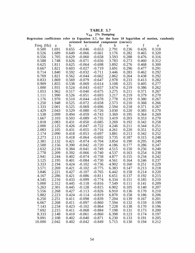
54
TABLE 3.7Vea 2% Damping
Regression coefficients refer to Equation 3.7, for the base 10 logarithm of motion, randomlyoriented horizontal component (cm/sec)
Freq. (Hz) a b c d h e f σ 0.500 1.691 0.655 -0.046 -0.653 2.791 0.236 0.426 0.318 0.526 1.689 0.649 -0.066 -0.661 3.176 0.282 0.465 0.320 0.556 1.705 0.629 -0.060 -0.658 3.593 0.288 0.476 0.316 0.588 1.748 0.626 -0.071 -0.656 3.783 0.273 0.460 0.312 0.625 1.811 0.625 -0.064 -0.698 3.892 0.276 0.468 0.300 0.667 1.821 0.603 -0.027 -0.719 3.691 0.296 0.477 0.291 0.714 1.840 0.592 -0.032 -0.711 3.446 0.283 0.462 0.292 0.769 1.821 0.562 -0.044 -0.662 2.862 0.264 0.438 0.292 0.833 1.869 0.569 -0.079 -0.647 2.978 0.233 0.413 0.282 0.909 1.855 0.538 -0.069 -0.614 3.108 0.225 0.405 0.277 1.000 1.931 0.524 -0.043 -0.657 3.674 0.219 0.386 0.262 1.053 1.962 0.517 -0.040 -0.675 3.275 0.211 0.371 0.267 1.111 1.990 0.526 -0.051 -0.693 3.217 0.219 0.379 0.270 1.176 1.970 0.510 -0.044 -0.678 2.778 0.219 0.380 0.267 1.250 1.948 0.525 -0.072 -0.658 2.573 0.210 0.368 0.266 1.333 2.001 0.525 -0.069 -0.696 2.594 0.218 0.371 0.267 1.429 2.043 0.529 -0.080 -0.726 3.030 0.220 0.385 0.270 1.538 2.099 0.494 -0.059 -0.743 3.369 0.195 0.364 0.269 1.667 2.103 0.503 -0.089 -0.735 3.419 0.203 0.353 0.270 1.818 2.083 0.431 -0.050 -0.685 3.269 0.192 0.342 0.258 2.000 2.125 0.426 -0.047 -0.722 4.246 0.211 0.344 0.251 2.083 2.105 0.431 -0.055 -0.716 4.261 0.220 0.351 0.252 2.174 2.090 0.418 -0.053 -0.697 3.881 0.213 0.342 0.252 2.273 2.113 0.418 -0.064 -0.692 3.735 0.187 0.315 0.248 2.381 2.132 0.421 -0.074 -0.704 3.854 0.190 0.295 0.249 2.500 2.156 0.390 -0.042 -0.720 4.186 0.177 0.286 0.247 2.632 2.218 0.384 -0.041 -0.749 4.515 0.150 0.256 0.240 2.778 2.209 0.392 -0.066 -0.740 4.537 0.163 0.254 0.238 2.941 2.244 0.402 -0.074 -0.758 4.877 0.155 0.234 0.242 3.125 2.195 0.401 -0.084 -0.730 4.561 0.164 0.246 0.237 3.333 2.194 0.424 -0.102 -0.736 4.902 0.160 0.251 0.229 3.571 2.269 0.421 -0.102 -0.775 6.383 0.147 0.213 0.218 3.846 2.221 0.427 -0.107 -0.765 6.442 0.158 0.214 0.220 4.167 2.286 0.421 -0.086 -0.811 6.651 0.137 0.192 0.215 4.545 2.216 0.433 -0.099 -0.774 6.334 0.151 0.185 0.210 5.000 2.312 0.445 -0.118 -0.816 7.549 0.111 0.141 0.209 5.263 2.301 0.445 -0.128 -0.815 6.902 0.105 0.140 0.207 5.556 2.268 0.427 -0.113 -0.826 6.910 0.136 0.170 0.210 5.882 2.223 0.424 -0.114 -0.819 6.870 0.158 0.186 0.206 6.250 2.251 0.411 -0.098 -0.839 7.204 0.139 0.167 0.201 6.667 2.268 0.411 -0.097 -0.860 7.594 0.132 0.159 0.199 7.143 2.234 0.423 -0.102 -0.864 7.228 0.138 0.170 0.196 7.692 2.215 0.411 -0.068 -0.884 7.198 0.131 0.173 0.200 8.333 2.148 0.410 -0.061 -0.860 6.398 0.123 0.174 0.197 9.091 2.108 0.402 -0.040 -0.871 6.230 0.133 0.191 0.20510.000 2.042 0.402 -0.042 -0.849 5.715 0.130 0.194 0.212

55
TABLE 3.8Vea 5% Damping
Regression coefficients refer to Equation 3.7, for the base 10 logarithm of motion, randomlyoriented horizontal component (cm/sec)
Freq. (Hz) a b c d h e f σ 0.500 1.686 0.637 -0.050 -0.646 2.873 0.250 0.435 0.293 0.526 1.698 0.630 -0.059 -0.651 3.175 0.272 0.454 0.294 0.556 1.715 0.618 -0.062 -0.651 3.474 0.279 0.464 0.290 0.588 1.747 0.613 -0.068 -0.655 3.622 0.277 0.462 0.287 0.625 1.785 0.606 -0.057 -0.677 3.653 0.278 0.464 0.280 0.667 1.808 0.591 -0.039 -0.696 3.570 0.289 0.469 0.273 0.714 1.824 0.577 -0.041 -0.687 3.307 0.278 0.453 0.272 0.769 1.824 0.561 -0.055 -0.653 2.921 0.260 0.432 0.269 0.833 1.855 0.554 -0.073 -0.642 2.961 0.242 0.416 0.262 0.909 1.862 0.528 -0.061 -0.627 3.161 0.234 0.407 0.255 1.000 1.915 0.520 -0.050 -0.648 3.330 0.218 0.381 0.247 1.053 1.947 0.519 -0.050 -0.667 3.240 0.213 0.372 0.249 1.111 1.971 0.517 -0.050 -0.682 3.163 0.215 0.373 0.250 1.176 1.962 0.513 -0.053 -0.675 2.897 0.217 0.374 0.248 1.250 1.960 0.516 -0.064 -0.669 2.704 0.212 0.369 0.247 1.333 1.996 0.514 -0.065 -0.694 2.764 0.212 0.368 0.249 1.429 2.029 0.506 -0.066 -0.713 3.055 0.211 0.372 0.253 1.538 2.069 0.490 -0.065 -0.726 3.324 0.200 0.361 0.252 1.667 2.077 0.483 -0.078 -0.718 3.439 0.202 0.350 0.249 1.818 2.074 0.439 -0.054 -0.694 3.502 0.199 0.339 0.241 2.000 2.091 0.427 -0.050 -0.707 4.134 0.211 0.340 0.236 2.083 2.081 0.426 -0.055 -0.700 4.119 0.212 0.339 0.236 2.174 2.080 0.421 -0.058 -0.692 3.985 0.204 0.328 0.235 2.273 2.093 0.416 -0.063 -0.690 3.937 0.192 0.310 0.233 2.381 2.107 0.412 -0.065 -0.696 3.988 0.187 0.295 0.232 2.500 2.131 0.399 -0.056 -0.710 4.215 0.178 0.283 0.230 2.632 2.160 0.393 -0.056 -0.721 4.398 0.162 0.263 0.227 2.778 2.175 0.397 -0.068 -0.728 4.561 0.162 0.252 0.225 2.941 2.194 0.400 -0.077 -0.737 4.868 0.159 0.241 0.224 3.125 2.180 0.405 -0.087 -0.729 4.868 0.162 0.242 0.221 3.333 2.182 0.420 -0.099 -0.735 5.170 0.161 0.241 0.215 3.571 2.213 0.425 -0.106 -0.754 6.042 0.154 0.219 0.207 3.846 2.204 0.426 -0.105 -0.761 6.330 0.157 0.212 0.205 4.167 2.233 0.425 -0.095 -0.787 6.468 0.144 0.195 0.203 4.545 2.210 0.433 -0.102 -0.777 6.522 0.145 0.181 0.199 5.000 2.262 0.442 -0.117 -0.803 7.261 0.122 0.153 0.199 5.263 2.257 0.440 -0.121 -0.807 7.026 0.120 0.152 0.198 5.556 2.240 0.431 -0.115 -0.815 7.070 0.134 0.166 0.198 5.882 2.222 0.424 -0.109 -0.823 7.155 0.148 0.178 0.196 6.250 2.225 0.417 -0.099 -0.836 7.297 0.142 0.172 0.193 6.667 2.228 0.417 -0.097 -0.848 7.368 0.134 0.164 0.191 7.143 2.203 0.419 -0.091 -0.855 7.212 0.134 0.169 0.190 7.692 2.176 0.416 -0.072 -0.866 6.935 0.130 0.174 0.193 8.333 2.123 0.413 -0.060 -0.855 6.425 0.125 0.178 0.194 9.091 2.079 0.412 -0.049 -0.857 6.184 0.132 0.190 0.20010.000 2.027 0.413 -0.047 -0.846 5.804 0.132 0.197 0.207

56
TABLE 3.9Vea 10% Damping
Regression coefficients refer to Equation 3.7, for the base 10 logarithm of motion, randomlyoriented horizontal component (cm/sec)
Freq. (Hz) a b c d h e f σ 0.500 1.712 0.610 -0.048 -0.643 3.040 0.256 0.436 0.269 0.526 1.727 0.605 -0.053 -0.646 3.219 0.265 0.445 0.268 0.556 1.742 0.598 -0.057 -0.648 3.384 0.272 0.451 0.266 0.588 1.764 0.592 -0.058 -0.653 3.468 0.275 0.453 0.264 0.625 1.790 0.584 -0.053 -0.663 3.481 0.275 0.453 0.260 0.667 1.813 0.574 -0.047 -0.672 3.419 0.275 0.450 0.256 0.714 1.831 0.562 -0.048 -0.666 3.263 0.267 0.438 0.254 0.769 1.843 0.549 -0.057 -0.651 3.055 0.255 0.424 0.250 0.833 1.862 0.538 -0.064 -0.640 3.052 0.243 0.411 0.245 0.909 1.883 0.521 -0.057 -0.637 3.189 0.234 0.399 0.240 1.000 1.921 0.512 -0.052 -0.650 3.272 0.222 0.380 0.235 1.053 1.944 0.510 -0.052 -0.661 3.239 0.217 0.372 0.235 1.111 1.962 0.507 -0.052 -0.670 3.160 0.215 0.369 0.235 1.176 1.970 0.504 -0.055 -0.673 3.049 0.214 0.366 0.234 1.250 1.981 0.502 -0.058 -0.678 2.972 0.212 0.363 0.234 1.333 2.003 0.498 -0.060 -0.691 3.015 0.210 0.362 0.235 1.429 2.031 0.490 -0.062 -0.704 3.192 0.208 0.360 0.238 1.538 2.058 0.479 -0.064 -0.712 3.408 0.203 0.353 0.237 1.667 2.070 0.465 -0.067 -0.709 3.555 0.202 0.344 0.235 1.818 2.076 0.440 -0.057 -0.701 3.761 0.203 0.336 0.229 2.000 2.083 0.427 -0.055 -0.702 4.109 0.205 0.330 0.226 2.083 2.084 0.423 -0.057 -0.699 4.154 0.203 0.325 0.224 2.174 2.085 0.419 -0.060 -0.695 4.132 0.199 0.316 0.223 2.273 2.090 0.415 -0.063 -0.693 4.112 0.193 0.305 0.222 2.381 2.100 0.409 -0.064 -0.696 4.159 0.187 0.293 0.220 2.500 2.116 0.403 -0.063 -0.702 4.286 0.179 0.280 0.218 2.632 2.134 0.399 -0.065 -0.710 4.430 0.169 0.266 0.216 2.778 2.151 0.401 -0.071 -0.718 4.618 0.165 0.254 0.215 2.941 2.163 0.404 -0.079 -0.725 4.855 0.162 0.245 0.213 3.125 2.168 0.409 -0.087 -0.729 5.079 0.162 0.239 0.210 3.333 2.172 0.418 -0.097 -0.734 5.357 0.161 0.233 0.206 3.571 2.185 0.422 -0.102 -0.745 5.848 0.156 0.220 0.200 3.846 2.193 0.424 -0.102 -0.757 6.185 0.152 0.208 0.197 4.167 2.201 0.427 -0.101 -0.770 6.384 0.145 0.195 0.195 4.545 2.206 0.431 -0.105 -0.778 6.624 0.140 0.181 0.192 5.000 2.227 0.436 -0.112 -0.796 7.049 0.130 0.164 0.191 5.263 2.228 0.435 -0.114 -0.804 7.092 0.129 0.164 0.191 5.556 2.220 0.431 -0.111 -0.812 7.117 0.135 0.168 0.190 5.882 2.209 0.426 -0.106 -0.820 7.172 0.141 0.174 0.189 6.250 2.200 0.422 -0.100 -0.827 7.175 0.140 0.173 0.188 6.667 2.189 0.421 -0.095 -0.835 7.140 0.137 0.172 0.187 7.143 2.170 0.419 -0.087 -0.843 7.004 0.135 0.174 0.187 7.692 2.142 0.419 -0.075 -0.849 6.745 0.132 0.178 0.189 8.333 2.103 0.417 -0.064 -0.847 6.399 0.129 0.183 0.192 9.091 2.059 0.416 -0.054 -0.845 6.064 0.131 0.191 0.19710.000 2.013 0.419 -0.050 -0.839 5.746 0.132 0.199 0.204

57
TABLE 3.10
Modal Events for the Point Source Example
PSV VeaP(G>g) = 1/2,500, 60 km
Freq. g m ' m εεεε g m ' m εεεε 0.5 16.7 7.46 7.08 1.12 30.6 7.46 7.03 1.20
1.0 19.0 7.30 7.03 1.24 34.1 7.46 6.97 1.28
2.0 15.8 7.03 6.70 1.68 31.8 7.30 7.03 1.24
3.0 13.8 6.70 6.54 1.80 29.8 7.03 6.86 1.40
4.0 10.8 6.59 6.50 1.80 25.5 7.03 6.86 1.40
5.0 9.9 6.49 6.43 1.80 24.8 6.97 6.81 1.44
6.7 6.6 6.38 6.27 1.96 18.5 7.03 6.92 1.32
P(G>g) = 1/500, 10 km
Freq. g m ' m εεεε g m ' m εεεε 0.5 24.9 6.86 6.49 1.00 40.0 6.86 6.54 0.88
1.0 33.5 6.70 6.38 1.16 52.6 6.86 6.54 0.88
2.0 34.0 6.54 6.22 1.36 59.1 6.76 6.32 1.24
3.0 32.7 6.32 6.11 1.44 61.0 6.59 6.27 1.28
4.0 27.1 6.27 6.16 1.32 55.1 6.65 6.43 1.00
5.0 24.8 6.27 6.16 1.28 54.2 6.65 6.32 1.16
6.7 17.8 6.16 6.00 1.48 43.6 6.65 6.43 1.00

58
TABLE 3.11
Modal Events for the Example of Combined Background and Line Source
Background
PSV VeaFreq. g ( m ', r ' ) ( m , r , εεεε ) g ( m ', r ' ) ( m , r , εεεε )
0.5 24.5 (6.48, 6.5) (6.43, 10.5, 1.08) 43.0 (6.48,6.5) (6.48, 10.5, 1.12)
1.0 27.9 (6.43, 6.5) (6.23, 8.5, 0.92) 47.2 (6.48, 7.5) (6.43, 11.5, 1.00)
2.0 25.0 (5.92, 5.5) (5.58, 5.5, 1.16) 46.1 (6.28, 6.5) (5.93, 7.5, 1.12)
3.0 22.8 (5.73, 5.5) (5.63, 7.5, 1.16) 44.8 (6.24, 6.5) (5.83, 7.5, 1.08)
6.7 12.0 (5.93, 9.5) (5.73, 10.5, 1.16) 28.8 (6.23, 8.5) (6.03, 9.5, 0.72)
Line Source
Freq. g ( m ', r ' ) ( m , r , εεεε ) g ( m ', r ' ) ( m , r , εεεε )0.5 24.5 (7.38, 30.5) (6.98, 30.5, 1.16) 43.0 (7.38, 30.5) (7.08, 30.5, 0.96)
1.0 27.9 (7.28, 30.5) (6.98, 30.5, 1.12) 47.2 (7.28, 30.5) (6.93, 30.5, 1.16)
2.0 25.0 (6.93, 30.5) (6.73, 30.5, 1.52) 46.1 (7.13, 30.5) (6.93, 30.5, 1.16)
3.0 22.8 (6.48, 30.5) (6.48, 30.5, 1.76) 44.8 (6.88, 30.5) (6.73, 30.5, 1.40)
6.7 12.0 (6.43, 30.5) (6.38, 30.5, 1.76) 28.8 (6.93, 30.5) (6.78, 30.5, 1.24)

59
Chapter 4: Results and Conclusions
The solutions of many earthquake engineering problems involve dynamic analyses using
ground-motion time series. The time series, or design earthquake, should be selected to reflect the
characteristics of potential ground-motion at a specific site. Important characteristics include
amplitude of motion, frequency content and duration of shaking, all of which are highly dependent
upon the magnitude and distance of the earthquake. In most cases, a complete assessment of the
seismic hazard must take into account the possible occurrence of earthquakes covering a range of
magnitudes, and occurring at several possible distances from a given site.
The design earthquake selection problem is fundamentally probabilistic. A rational and
objective apporach to the solution can involve disaggregation of a formal probabilistic model of the
seismic hazard. The disaggregation can identify the most likely earthquake scenario(s), in terms of
magnitude and distance, that contribute to hazard, for any specified return period. An ensemble of
time series for different harmonic oscillators can be selected on the basis of the modal earthquakes
derived from the analysis. This gives a useful time-domain realization of the seismic hazard, to the
extent that important characteristics of the time series are correlated with the basis variable used in
the analysis. A limitation may arise because most currently available motion prediction models are
essentially independent of duration, and modal events based on PSHA disaggregation using peak
elastic response as the basis variable for the analysis may not represent the optimal characterization
of the hazard.
The elastic input energy spectrum is an attractive alternative to the elastic response spectrum for
these types of analyses. The input energy combines the elements of amplitude and duration into a
single parameter description of the ground motion that can be readily incorporated into standard
PSHA methodology. This use of the elastic input-energy spectrum was examined, using strong
motion data from Western North America. Regression modeling using consistent processing
procedures for the absolute input energy equivalent velocity Vea, and the elastic response PSV in
the frequency range 0.5 to 10 Hz shows that the two parameters can be successfully fit with
identical functional forms. The variance of Vea is uniformly less than that of PSV, indicating that
Vea can be predicted with slightly less uncertainty, as a function of magnitude, distance and site
classification. The dependence of Vea and PSV upon NEHRP site classification (BSSC, 1994) is
virtually identical. The effects of site class are important at frequencies less than a few Hertz. The

60
regression modeling does not resolve significant effects due to site class at frequencies greater than
approximately 5 Hz. These results are illustrated in Figures 3.7 through 3.9.
The elastic input energy offers a potential advantage over the elastic response spectrum in that it
reflects, by integration, the effect of ground motion duration. This is evident in the regression
models by a stronger magnitude scaling of Vea, compared to PSV, for oscillator frequencies
greater than approximately 2 Hz (Figures 3.9 through 3.11). The implication for probabilistic
hazard analysis is that if the hazard is assessed on the basis of Vea, the hazard posed by the larger
magnitude earthquakes contributes more to the total hazard, than would be the case if the
assessment where done on the basis of the elastic response spectrum. Disaggregation of simple,
fairly general, seismic hazard models using Vea indicates that the modal magnitudes for the higher
frequency oscillators tend to be larger, and vary less with oscillator frequency, than those derived
using PSV (Figures 3.12 and 3.13). Insofar as the elastic input-energy may be a better parameter
for quantifying the damage potential of ground motion, its use in probabilistic seismic hazard
analysis could provide an improved means for selecting earthquake scenarios and establishing
design earthquakes for many types of engineering analyses.

61
Bibliography
Abrahamson, N. A. and K. M. Shedlock (1997). Some comparisons between recent ground-
motion relations, Seismological Research Letters, 68, 9-23.
Bazzurro, P. and C. A. Cornell (1998). On disaggregation of seismic hazard, submitted to Bull.
Seism. Soc. Am., 1998.
Bender, B. (1984). Seismic hazard estimation using a finite-fault rupture model, Bull. Seism. Soc.
Am. 74, 1899-1923.
Bernreuter, D. L., J. B. Savy, R. W. Mensing and J. C. Chen (1989). Seismic Hazard
Characterization of 69 Nuclear Power Plant Sites East of the Rocky Mountains. U. S.
Nuclear Regulatory Commission, NUREG/CR-5250.
Boore, D. M., W. B. Joyner, and T. E. Fumal (1997). Equations for estimating horizontal
response spectra and peak acceleration from western North American earthquakes: a
summary of recent work, Seismological Research Letters, 88, no. 1, 128-153.
Boore, D. M., W. B. Joyner, and T. E. Fumal (1994). Estimation of response spectra and peak
accelerations from western North American earthquakes: An interim report, Part 2, U.S.
Geol. Survey Open-File Report, 94-127, 40 pp.
Boore, D. M., W. B. Joyner, and T. E. Fumal (1993). Estimation of response spectra and peak
accelerations from western North American earthquakes: An interim report, U.S. Geol.
Survey Open-File Report, 93-509, 72 pp.
BSSC (1994). NEHRP recommended provisions for seismic regulations for new buildings, Part 1
- Provisions, FEMA 222A, Federal Emergency Management Agency, 290 pp.
Campbell, K. W. (1997). Empirical near-source attenuation relationships for horizontal and
vertical components of peak ground acceleration, peak ground velocity, and pseudo-
absolute acceleration response spectra, Seismological Research Letters, 68, 154-179.
Chapman, M. C. (1995) A probabilistic approach to ground-motion selection for engineering
design, Bull. Seism. Soc. Am., 85, 937-942.
Cockerham, R. S., and J. P. Eaton (1987). The earthquake and its aftershocks, April 24 through
September 30, 1984, in The Morgan Hill, California Earthquake of April 24, 1984, U. S.,
Geological Survey Bulletin 1639, 15-28.
Coppersmith, K. J. and R. R. Youngs (1986) Capturing uncertainty in probabilistic seismic hazard
assessments within intraplate tectonic environments, Proceedings of the Third U. S.
National Conference on Earthquake Engineering, Charleston, SC, 1, 301-312.
Cornell, C. A. (1968). Engineering seismic risk analysis, Bull. Seism. Soc. Am., 58, 1583-1606.

62
Cramer C. H. and M. D. Petersen (1996). Predominant seismic source distance and magnitude
maps for Los Angeles, Orange and Ventura Counties, California, Bull. Seism. Soc. Am.,
86, 1645-1649.
Frankel, A., C. Mueller, T. Barnhard, D. Perkins E. V. Leyendecker, N. Dickman, S. Hanson
and M. Hopper (1996). National Seismic-Hazard Maps: Documentation June 1996, U. S.
Geological Survey Open-File Report 96-532, Denver, CO.
Gutenberg, B., and C. F. Richter (1954). Seismicity of the Earth, Princeton University Press,
2nd ed., pp. 16-25.
Harmsen, S. C. (1997). Determination of site amplification in the Los Angeles urban area from
inversion of strong-motion records, Bull. Seism. Soc. Am., 87, 866-887.
Hauksson, E., (1994). The 1991 Sierra Madre earthquake sequence in southern California:
seismological and tectonic analysis, Bull. Seism. Soc. Am., 84, 1058-1074.
Joyner, W. B. and D. M. Boore (1993). Methods for regression analysis of strong-motion data,
Bull. Seism. Soc. Am., 83, 469-487.
Joyner, W. B. and D. M. Boore (1994). Errata, Bull. Seism. Soc. Am., 84, 955-956.
Joyner, W. B. and D. M. Boore (1982). Prediction of earthquake response spectra, U. S. Geol.
Surv. Open File Report 82-977.
Lawson, R. S., (1996) Site Dependent Inelastic Seismic Demands , Ph.D. dissertation,
Department of Civil Engineering, Stanford University, Stanford, CA, 224 p.
McGuire, R. K. (1995). Probabilistic seismic hazard analysis and design earthquakes: Closing the
loop, Bull. Seism. Soc. Am., 85, 1275-1284.
McGuire, R. K. and K. M. Shedlock (1981). Statistical uncertainties in seismic hazard evaluations
in the United States, Bull. Seism. Soc. Am., 71, 1287-1308.
Milne, W. G. and D. H. Weichert (1986) Seismic ground-motion computations at low
probabilities, Can. J. Civ. Eng. 13, 595-599.
National Research Council (1988). Proababilistic Seismic Hazard Assessment, National
Academy Press, Washington, D.C.
Nigam, N. C. and P. C. Jennings (1969). Calculation of response spectra from strong-motion
earthquake records, Bull. Seism. Soc. Am., 59, 909-922.
Reiter, L. (1990). Earthquake Hazard Analysis: Issues and Insights, Columbia Univ. Press,
New York.
Sharp, R. V., M. J. Rymer and J. J. Lienkaemper (1986). Surface displacement on the Imperial
and Superstition Hill faults triggered by the Westmoreland, California earthquake of 26
April 1981, Bull. Seism. Soc. Am., 76, 949-965.
63
Stepp, J. C., W. J. Silva, R. K. McGuire and R. T. Sewell (1993). Determination of earthquake
design loads for a high level nuclear waste repository facility, in Proc., 4th DOE Natural
Phen. Haz. Mitig. Conf., Vol. 2, Atlanta, GA, 651-657.
Woo, G. (1996). Kernel estimation methods for seismic hazard area source modeling, Bull.
Seism. Soc. Am., 86, 353-362.
Working Group on California Earthquake Probabilities (1995). Seismic hazards in southern
California: Probable earthquakes, 1994-2024, Bull. Seism. Soc. Am., 85, 379-439.
Yeats, R. S., K. Sieh and C. R. Allen (1997) The Geology of Earthquakes, Oxford Univ. Press,
New York, 568 p.
Youngs, R. R. and K. J. Coppersmith (1985) Implications of fault slip rates and earthquake
recurrence models to probabilistic seismic hazard estimates, Bull. Seism. Soc. Am., 75,
939-964.
Uang, C.-M. and V. V. Bertero (1990). Evaluation of seismic energy in structures, Earthquake
Engineering and Structural Dynamics, 19, 77-90.
Wald, D. J. and T. H. Heaton (1994). Spatial and temporal distribution of slip for the 1992
Landers, California, earthquake, Bull. Seism. Soc. Am., 84, 668-691.
Wald, D. J., T. H. Heaton and K. W. Hudnut (1996). The slip history of the 1994 Northridge,
California, earthquake determined from strong-motion, teleseismic, GPS, and leveling
data, Bull. Seism. Soc., Am., 86, no. 1B, 49-70.
Wessel, P., and W.H.F. Smith (1991). Free software helps map and display data, EOS Trans.
Amer. Geophys. U., 72, 441, 445-446.

64
Vita
Martin C. Chapman
165 Greenway Drive
Christiansburg, VA, 24073
Education:
B.S., Geophysics, Virginia Polytechnic Institute and State University, Blacksburg VA, 1977.
M.S., Geophysics, Virginia Polytechnic Institute and State University, Blacksburg VA, 1979.
Ph.D., Geophysics, Virginia Polytechnic Institute and State University, Blacksburg VA, 1998.
Professional Experience:
Geophysicist, Law Engineering Testing Company, Marietta GA, (1979-1984).
Research Associate Dept. Geological Sciences, Virginia Polytechnic Institute and State
University, Blacksburg, VA, (1984-Present).


![Monetary Policy and Real Estate Prices: A Disaggregated ... · PDF fileReal Estate Prices: A Disaggregated Analysis for Switzerland ... Dupor [2005] analyzes in ... A Disaggregated](https://img.pdfslide.us/doc/110x75/5a79a5d87f8b9ae1468d0da8/monetary-policy-and-real-estate-prices-a-disaggregated-estate-prices-a-disaggregated.jpg)