DISAGGREGATE WEALTH AND AGGREGATE CONSUMPTION: AN

INVESTIGATION OF EMPIRICAL RELATIONSHIPS FOR THE G7

Joseph P. Byrne and E. Philip Davis1

1st Version: January 2001

This Version: October 11th 2001

Abstract: To date, testing for wealth effects in consumption has mainly used aggregate wealth definitions,

and/or is on a single-country basis. This study breaks new ground by analysing disaggregated wealth in

consumption functions for G7 countries. Contrary to other empirical work, illiquid financial wealth, (securities,

pensions and mortgage debt), tends to be a more significant long-run determinant of consumption than liquid

financial wealth. We suggest that this pattern reflects a shift from liquidity constrained to life cycle behaviour

following financial liberalisation. Results were robust in SURE analysis, tested in a nested manner, using

varying definition of liquid assets and using non-property income instead of personal disposable income. Wald

tests indicate similar long-run behaviour for all EU countries including the UK.

Keywords: consumers’ expenditure; disaggregate household wealth; SURE; G7.

JEL Classification: E21; F15.

Words: 11532

1 Joseph Byrne is an economist at the National Institute of Economic and Social Research, 2 Dean Trench Street, Smith Square, London, SW1P 3HE, e-mail jbyrne@niesr.ac.uk while E Philip Davis is Professor of Economics and Finance, Brunel University, Uxbridge, Middlesex, UB8 3PH and a Visiting Fellow at NIESR. E-mails, philip.davis@brunel.ac.uk and e_philip_davis@msn.com The authors wish to thank Paul Ashworth, Ray Barrell, Nigel Pain and Martin Weale for helpful comments on earlier drafts. All errors or omissions are the responsibility of the authors.

2

1. Introduction

Amongst the numerous studies of consumer expenditure,2 the issue of the existence

and size of wealth effects in the consumption function has come to the fore strongly in recent

years. This is partly a consequence of the strength of consumption and low level of savings in

the United States in the late 1990s (see inter alia Ludvigsen and Steindel, 1999, Poterba,

2000, and IMF, 2000), which is often thought to be linked to rising share prices and resultant

wealth effects.3 A major fall in equity prices could conversely lead to a sharp fall in

consumption with wider effects on the macroeconomy. Equally, strong shifts in asset prices,

as in Scandinavia and the UK in the late 1980s and early 1990s, may have amplified the

business cycle partly via wealth effects on consumption, linked to credit expansion (Berg and

Bergstrom, 1995, and Davis, 1995). Similar arguments may apply to the current weakness of

consumption in Japan.

In more detail, wealth effects on consumption generally are coming increasingly to the

fore, firstly owing to macroeconomic trends. The ratio of wealth to income and consumption

is rising in the major industrial economies, suggesting that the ability to draw on wealth to

maintain consumption is increasing (see Charts 8-14 discussed in Section 3). But there are

also reasons for interest in disaggregated wealth, such as the aforementioned recent pattern of

negative saving in the US accompanying rapid consumption growth. In terms of

macroeconomic policy, the link from wealth to consumption gives a reason for interest in the

effect of asset prices on the aggregate economy. Hence the possible need for monetary policy

makers to focus on asset prices as well as consumer prices (Gertler et al., 1998, and

Woodford, 1994).4 The case is strengthened by the role of asset prices in “credit cycles” in the

late 1980s. An attempt at disaggregation can cast further light on these issues by highlighting

2 See Muellbauer and Lattimore (1995) for a comprehensive survey of empirical work on consumption. 3 In the US between 1994 and 1997 alone, the value of household sector equity holdings doubled. 4 See also the Federal Reserve Bank of Kansas City’s (1999) symposium on asset prices and monetary policy at

Jackson Hole and Stock and Watson (2001).

3

which asset prices are most relevant for consumption. There could also be light cast on

whether households react to the variance as well as the mean level of asset prices and

resultant values of their assets (i.e. whether they react strongly to increased risk).

Financial liberalisation may lead to changes in wealth effects. Free availability of

credit may reduce the importance of income as a determinant of consumption. Borrowing may

develop a strong independent, and at times even positive, effect on consumption, which may

not be consistent with conventional consumption functions, which assume a negative sign for

borrowing in the construction of net wealth. In this context, the effect of debt on consumption

might also differ according to the level of gearing and the stage of the business cycle, being

favourable to consumption at low levels of borrowing, but negative when there is high gearing

and a downturn in the economy. Or, as suggested by De Bondt (1999), there may be effects

on consumption operating via the “credit channel” and the cost of external finance, which will

in turn relate to the gearing of the household sector. Meanwhile, the rise in home ownership

offers a sizeable asset to an increasing number of households, against which the value of

which they may borrow at relatively low cost compared to unsecured consumer credit.

However, if such borrowing becomes sizeable, there may be repercussions (negative equity)

when house prices fall, which may dampen consumption while households correct their

balance sheets, to a degree in excess of that expected from prior relationships.

The institutionalisation of saving, and in particular the growing share of household

wealth held in the form of life insurance and pension funds (Davis and Steil 2001), raises the

question of whether the relative illiquidity of such wealth may give it a weaker wealth effect

than directly held and liquid wealth. On the other hand, the decreasing elements of insurance

(e.g. in the shift from defined benefit to defined contribution pension funds) which would

otherwise insulate the beneficiary from asset price changes, could increase the wealth effect

from this source. Linking to this, the ageing of the population is helping to drive an increased

accumulation of wealth, independent of other motives for saving. There is an interest in how

4

consumption will evolve as population ageing and related accumulation of assets proceeds.

Possibly the time horizon over which consumers expect to de-cumulate their asset holdings

may vary, which in turn might affect the size of the wealth effects.

A number of recent studies have as a consequence of these developments investigated

the properties of total net wealth as a determinant of consumption. However, rather fewer

studies have sought to disaggregate wealth and assess whether rises in sub-components of

wealth have differential effects on consumption. And even those that do attempt this are rarely

undertaken on a comparative, cross-country basis or with sectoral balance sheet data as

opposed to proxies using asset prices. This paper hence seeks to break new ground by

presenting and comparing data and estimates of the relation between components of personal

or household sector wealth and consumers’ expenditure for the US, UK, Germany, France,

Italy, Japan and Canada. We basically employ a backward looking specification for aggregate

consumption where the long-run relationship between consumption, income and wealth is

estimated within an error correction model. We then seek to disaggregate the existing long-

run wealth terms within our established short-run model. We consequently test whether the

typical imposition of an equivalent long-run elasticity for the components of wealth is

consistent with the data. Differences in the impact of the components of wealth have been

found by a few papers studying US consumption. For example, Brayton and Tinsley (1996)

find that the marginal propensity to consume out of stock market wealth is less than half that

out of other types of wealth. We examine whether this kind of result stands up for other G7

countries and in doing so we can compare similarities of the major European countries.

The paper is structured as follows. In Section Two we illustrate the data currently

available for the G7 countries, showing major contrasts and common trends within the

balance sheet of the household sector. In the third section we briefly note the theoretical

background which could justify inclusion of wealth in a consumption function, and

implications of its disaggregation; the section also looks at recent empirical work on wealth

5

effects in consumption, which including extant work disaggregating wealth (usually on a

single country basis). The fourth section presents our own results. In the conclusion we seek

to draw out some underlying features and policy implications of these outturns.

2. Patterns of Wealth Holding in the G7

Whereas the points highlighted in the introduction apply to individual G-7 countries,

there are very marked differences in patterns of wealth holding across the G7, with in

particular a much lower level of equity and institutional holdings in Continental Europe than

in the English speaking countries. This could affect the responsiveness of consumption to

wealth via (i) similar coefficients on the components of wealth, but different size of the asset

components within the portfolio and/or (ii) different coefficients as well as different portfolio

composition. It is important to test for the relative importance of these effects via a

disaggregated wealth study, such as the work presented here, so as to calibrate correctly

wealth effects. Besides being relevant across groups of countries, any remaining differences

in wealth effects within Continental Europe will render more complex the task of the ECB to

conduct monetary policy. In this context, it is worth noting that EMU is widely seen as

leading to an increase in the relative importance of securities markets and institutional

investors (Davis, 1999).

We now go on to outline patterns in the data in more detail. Charts 1-7 present trends

in the composition of gross financial wealth in the G7. These are drawn from the National

Flow of Funds Balance Sheet tables prepared by the National Central Banks of France,

Germany, Italy, Japan and the US and by the National Statistical Offices in the UK and

Canada. There are a number of important differences in the time series behaviour of this data.

In particular, Canada, the UK and US show a higher proportion of institutional saving, while

liquid asset holdings tend to be lower. Over time this trend has grown in strength, with a sharp

decline in the share of liquid assets in the US from 25% up to the end of the 1980s down to

6

12% now. Over the same period equity holdings have risen from 15% to over 30% while long

term institutional saving has also risen from 23% to over 30%. In the UK, liquid asset

holdings have fallen from 40% of the portfolio in the early 1980s to 20% now, while life and

pension fund saving rose from 30% to over 50%, and equities from 15% to over 20%. In

Canada the shifts are less dramatic, but there is a rise in the share of life insurance and

pension funds from 30% to 40%, offset by falls in direct holdings of equities and bonds.

Underlying the decline in liquidity, besides relatively higher returns on capital uncertain

assets, is financial liberalisation, which has reduced the need for precautionary liquid asset

holdings.

On the other hand, differences between the Anglo Saxon countries and Continental

Europe should not be exaggerated, as there is some degree of convergence, which depending

on the coefficients in the consumption function could also imply a convergence of behaviour.

In particular, the share of liquid assets in France and Italy, which in the 1970s was over 60%

of gross personal sector financial assets, has now more than halved in response to rising

equity5 and institutional investment (in France) and rising equity and bond holdings (in Italy).

This pattern is also present in a muted form for Germany, where bond holdings have

increased relatively strongly. Japan is an exception in that liquidity has retained its

dominance, accounting for around 60% of portfolios in 1966 and 1998. Whereas convergence

had been apparent till 1990, the securities market crises of the 1990s have evidently driven

households back to low risk assets. Even the rise in life insurance and pension funds’ share

reached a plateau in the early 1990s.

It is also useful to consider patterns of aggregate wealth as a proportion of personal

disposable income (pdi). As shown in charts 8-14 there is a common pattern across all seven

countries of a rise in gross wealth relative to pdi, and a generally more muted rise in debt/pdi

ratios. Corresponding to these patterns, there has also been an increase in net wealth/pdi.

5 For France and Italy, data for equity include equity in non-corporate business, which is not included elsewhere.

7

The levels of the gross wealth ratio differ between around 5 for the US and UK and

around 3 for Continental Europe, Canada and Japan. While this no doubt partly relates to

differences in measurement, it may also link to the funded pension systems in the Anglo

Saxon countries shown in the wealth data, where a larger part of wealth of households in

France, Germany, Italy and Japan is in the form of implicit social security wealth. Meanwhile,

debt/pdi ratios are around 1 in Canada, the US, UK, Japan and Germany, while in France they

are around 0.6 and 0.3 in Italy. This partly reflects a cultural aversion to debt in Italy as well

as more recent financial liberalisation. In France debt ratio stood at around 0.8 in the late

1980s, and declined during the period of recession and falling asset prices of the early 1990s.

The German ratio may be exaggerated by inclusion of construction company liabilities along

with mortgage debt in the so-called “housing sector” of the financial accounts. A notable

feature of the UK in the 1990s is that the debt/pdi ratio has been flat after having risen sharply

in the 1980s mortgage-lending boom. In Japan the data include debt of unincorporated

businesses, which is sizeable.

3. Literature Review

3.1 Theoretical Background

We estimate benchmark consumption functions based on the Life Cycle Hypothesis

(LCH) of Ando and Modigliani (1963) as derived in Deaton (1992). In the LCH, planned

aggregate consumption ( *tC ) is a function of total resources. Total resources are the sum of

human wealth ( tH ) and net financial wealth ( 1−tW ). Therefore planned consumption can

consequently be expressed as

( )1*

−+= ttt WHmC (1)

where m is the marginal propensity to consume out of total resources on average across the

population. There are two difficulties with estimating equation (1) directly. First, planned

consumption does not always equal actual consumption owing inter alia to lags in adjustment,

8

which suggest using an error correction approach. Secondly, human wealth is unobservable

and typically proxied by some function of current labour income (i.e. tt kYH =~ ).

Consequently, we can derive the following, where tC is actual consumption and tC~ is target

consumption (equivalent to planned consumption but based on a specification using the

human wealth proxy, tH~ ):

ttt CC ε+=~ (2)

( ) tttt WHmC ε++= −1~ (3)

tttt bWaYC ε++= −1 (4)

Further modifications are warranted to estimate this specification of the consumption

function. As suggested by Campbell and Deaton (1989), income in levels is unlikely to be

difference stationary. In particular, the first difference of the level of income does not display

constant variance: earlier increases in the level of income, in any reasonable sample of data,

are likely to be substantially less than increases later in the sample. This non-constant

variance would mean our short run error correction model for consumption would have non-

stationary dynamics and the long-run relationship for consumption would potentially be

spurious, given that not all of our variables are difference stationary. Consequently we adopt a

logarithmic approximation for equation (4) to ensure that income, in natural logs, is difference

stationary and hence that our long-run relationship can be non-spurious. The logarithmic

approximation to equation (4) is as follows

( ) ( ) ( ) tttt WYcC ξβα +++= −10 lnlnln (5)

This is the approach adopted in recent work by Ludvigson and Steindel (1999), Davis and

Palumbo (2001), Lettau, Ludvigson and Barczi (2001) and Lettau and Ludvigson

(2001a,b,c,d). See also Campbell and Deaton (1989), Campbell and Mankiw (1991) and

Nelson (1987) for a fur ther discussion on logarithmic approximations of the aggregate life

cycle consumption function in equation (4).

9

A short run model which has a loglinear approximation of equation (4) as a

cointegrating vector can be derived from the work by Davidson, Hendry, Srba and Yeo

(1978). This approach nests consumption within an error correction term and allows for a

significant role for current income. Hendry von Ungern-Sternberg (1981) extended this paper

by including a measure of net wealth as an integral control mechanism. They derived a

consumption function from a utility maximisation problem with a quadratic loss function

thus:

[ ] [ ] [ ] [ ][ ]∗−

∗−−

∗∗ −−−−+−+−= 1142

132

22

1 2 ttttttttttt ccccccccwwq λλλλ (6)

An asterisk indicates the long run equilibrium level of consumption and wealth and all lower

case variables are in natural logs. The first two terms represent deviations of planned wealth

and consumption from target, the third term is adjustment costs and the fourth is a slippage

term. This solves to an error correction model of the form

( ) ( )11311210 −−−− −+−+∆+=∆ tttttt ywcyyc θθθθ (7)

Equation (7) can be reparameterised to produce a short run equation of the form

( )111110 −−− −−+∆+=∆ ttttt wycyc βαγθθ (8)

It should be noted that specification (8) incorporates equation (4) but wealth, income and

consumption are contemporaneously cointegrated. Below we estimate equation (8) as our

benchmark consumption function after including additional data-determined short run

dynamics.

The derivation above assumes that non-human wealth is homogeneous. However, this

is not the case either in terms of liquidity or capital certainty, which may suggest that the

effects of its sub-components on consumption may vary. Moreover, the household sector is

not homogeneous, for example in terms of (i) total wealth of households and (ii) stage of the

life cycle. Both of these may affect the portfolio composition of the household and its

response to changes in the components of wealth.

10

In this context, a priori, it is plausible that in a liquidity-constrained situation, net

liquid assets will strongly affect consumption, as well as disposable income. In such a

situation (i.e. where credit is not readily available), the liquidity of an asset is the key aspect

of its substitutability for consumer goods, and hence less liquid assets such as equities and life

and pension claims, will have a smaller effect on consumption than liquidity. Moreover, the

key component of net liquidity will be (gross) liquid assets rather than indebtedness,6 since

the latter is constrained ex hypothesi. (A similar argument holds for the income effect on

consumption, which will be large for liquidity constrained consumers.)

However, when liquidity constraints ease, both the importance of liquid assets and of

disposable income may well decline. The former will be less important than total wealth,

which indicates resources available over the life cycle for consumption, against which the

household may borrow. Whether there will be differences in the view taken by the household

in respect of types of wealth (and hence their weight in the consumption decision) is less clear

a priori, for the following reasons.

On the one hand, liquid assets will remain by definition a closer substitute for

consumption than illiquid ones, and especially contractual saving such as life and pension

fund claims. Also illiquid assets may be concentrated in fewer hands than liquid ones

(although this is less the case when there is a funded pension system). On the other hand, if

households tend to shift to a greater proportion of illiquid wealth as their overall wealth

increases and liquidity constraints ease (because they are willing to take higher risk on part of

the portfolio in exchange for higher return), the valuation of such illiquid wealth could come

to the fore as an indicator of consumption. Moreover, rises in debt as liquidity constraints ease

may also lead to a reduction in the measured effect of liquidity (since a rise in borrowing to

finance consumption gives a “negative wealth effect”). Meanwhile, disposable income will

6 Net liquid assets are typically defined to include total household debt as a negative variable (as it is a liability).

11

become at most an indicator of human wealth for life cycle purposes. It is the relative

importance of these arguments that this article seeks to test.

The above discussion has implications for the income variable used in consumption

function estimation. The conventional approach is to include real personal disposable income

in the consumption function. However, if wealth is to be included in the consumption

function, to avoid the risk of double counting it may be appropriate for one to omit property

income from the income variable, and use post tax income from employment and self

employment plus current grants minus social security contributions (see the discussion in

Muellbauer and Lattimore 1995). We evaluate both variables in our work reported in Section

4.

12

3.2 Aggregate Wealth

We now go on to assess recent empirical work on wealth and consumption, beginning

with specifications that do not disaggregate wealth. The inclusion of only liquid assets was the

typical practice in a number of early consumption functions following Hendry and von

Ungern Sternberg (1981) and earlier work such as Townend (1978) for the Bank of England

(see the survey in Davis, 1984). Income is in some of these studies adjusted for inflation

losses on net liquid assets (as part of interest payments, which enter personal disposable

income, are implicitly capital repayments). Alternatively, it has been popular to incorporate an

inflation variable which is a proxy for the capital loss on nominally denominated wealth in

periods of inflation (see Davidson et al. 1978, and recent expositions of the approach in

Pesaran et al., 1999, and Carruth et al., 1999).

This practice of focusing on nominal- fixed, liquid wealth was partly a consequence of

data limitations for illiquid wealth, but also expressed a view that liquid assets were in a sense

closer substitutes for consumption than illiquid wealth such as shares and pension wealth.

Liquid assets might be especially relevant when there are constraints on borrowing, and

indeed later practice has tended to use wider wealth aggregates, sometimes also including

housing wealth as well as financial wealth. Brodin and Nymoen (1992) show that financial

deregulation effects are well captured in Norway by the wealth variable.

According to Boone et al. (1998), Starr-McCluer (1998) and Brayton and Tinsley

(1996) studies of the US find that the MPC out of Net Wealth is between 1% and 7%. There is

no strong evidence of any wealth effect for France according to Bonner and Dubois (1995)

and Grunspan and Sicsic (1997), although Carruth (1999) finds evidence for a wealth effect

using an inflation proxy. Rossi and Visco (1995) find for Italy that the marginal propensity to

consume out of net wealth is equal to 3.5%. Generally, the literature finds weaker wealth

effects in Continental Europe and Japan than in the US, the UK and Canada.

13

Decisions about the construction of a wealth variable are dependent upon issues like

liquidity and intergenerational aggregation and lessons can be drawn from this literature when

examining disaggregate wealth. Liquidity considerations may suggest that different assets

have different weights in an aggregate measure. An increase in housing wealth for current

homeowners represents a decrease in future income for prospective homeowners. Muellbauer

and Lattimore (1995) find that house prices have a dual effect implied by theory: a positive

wealth effect (which depends on the degree of liquidity of housing) and a negative real price

effect. These effects may be different for different countries. Home ownership levels in

Europe range from 66% in the United Kingdom and 54% in France to 38% in Germany (see

Boone et al., 1998). The importance of housing wealth in the consumption function is

possibly a function of the level of home ownership. Housing wealth is not the only point of

contention with regards the impact of wealth’s components on consumption. For example,

stock market wealth is concentrated amongst the very wealthy who may have a relatively low

propensity to consume as wealth rises. Finally, Carroll (1994) demonstrates that on average

the level of consumption is closely related to current income and liquid assets rather than

measures of human wealth, suggesting that non-marketable wealth may not be particularly

related to consumption.

3.3 Disaggregated Wealth

One early study of disaggregate wealth by Pesaran and Evans (1984) suggested it was

insufficient to include solely capital gains and losses from liquid wealth in the consumption

function. They consequently developed a specification that also incorporates illiquid assets.

Estimating in terms of saving, they find superior results with their approach to that of

competing alternatives, with capital gains and losses being highly significant in explaining the

savings ratio, based on annual UK data between 1953-1981.

Recent work on disaggregation has included Boone et al. (1998), also explicitly

consider the effect of stock market wealth on consumption. They estimate a consumption

14

function for the US using financial wealth, which is based on the following linear

approximation to the equilibrium relationship in logarithmic form

cyt = a + ß(smwy)t + ?(nsmwy)t + other determinants

(9)

Where cyt is the consumption to income ratio (hence there is implicit imposition of

homogeneity), smwyt is the stock market wealth to income ratio and nsmwyt is non-stock

market wealth to income ratio (all variables are in logs). Stock market wealth consists of

corporate equities (held directly and those in close-end funds) plus mutual fund shares and life

insurance reserves. Due to difficulties obtaining reliable data for G7 countries other than the

US, Boone et al. (1998) use share prices to proxy capital gains and losses. The US marginal

propensity to consume is then re-scaled by the share of equities in disposable income for each

of the other countries. In their long-run specification for consumption the authors also

incorporate the real interest rate, the inflation rate and the unemployment rate as the other

determinants of the consumption income ratio. The real interest rate is included to take

account of substitution effects, the inflation rate to take account of uncertainty and real

depreciation of non- indexed financial assets, and thirdly the unemployment rate is included to

measure uncertainty surrounding the future stream of income. They incorporate the long-run

cointegrating relationship in a dynamic error correction model. Using the OECD macromodel

INTERLINK, they find significant real effects from a fall in G7 stock markets. For example

for the US a ten percent fall in stock market prices reduces consumption by 0.75 per cent after

allowing for indirect equity holdings, for the UK and Canada 0.45 and other G7 countries less

than 0.2.

Ludvigson and Steindel (1999) have also conducted a recent study of consumption in

the US where they differentiate between stock market wealth and non-stock market wealth.

Total wealth is household net wealth in billions of current dollars. Stock market wealth

includes direct household holdings, mutual fund holdings, holdings of private and public

15

pension plans, personal trusts and insurance companies. Using a loglinear specification to

avoid heteroskedasticity, they find evidence of similar impact from non-stock market wealth

and stock market wealth, for a sample period that runs from 1953Q1 to 1997Q4 (the elasticity

is approximately 0.04 for both effects) although they report some instability. However, the

estimated stock market effect is sensitive to the sample period chosen and there is some

evidence of instability from a likelihood ratio test. For a sample period that contains only ten

years of their most recent data the authors find a diminished stock market wealth effect

(elasticity is 0.21) and a negative elasticity on non-stock market wealth.

We have drawn attention to some of the issues involved when deciding the appropriate

definition of non-human wealth. Church et al. (1994) and Ogawa et al. (1996) emphasise that

we should differentiate according to the degree of liquidity. The US model of the FRB

emphasises the difference between (1) transfer wealth, (2) property wealth, (3) corporate

equity, and (4) other net financial and tangible asset wealth. (see Brayton and Tinsley, 1996).

The marginal propensity to consume out of stock market wealth is half of what the MPC is

out of other components of net wealth.

Regarding pension funds these are often considered as illiquid assets with a tenuous

effect on consumption. Nevertheless, Poterba and Samwick (1995) suggest that the

consumption patterns of those with pension plans exhibits a higher degree of correlation with

the stock market than those without. Equally, according to Starr-McCleur (1998) the

correlation between equity prices and aggregate activity has not been due to any direct stock

market effect. She uses survey data of US households and finds that any effect of the stock

market on saving and consumption behaviour arises primarily through retirement saving in

the form of mutual funds and retirement accounts. The rising trend of pension plan ownership

in the US and elsewhere would imply that it is pertinent to include pension funds in stock

market wealth when modelling consumption.

16

Housing is a form of wealth, not included in our work in this paper, partly for data

reasons; some researchers on individual countries have sought to include it in consumption

functions. Berg and Bergstrom (1995) disaggregate wealth as housing and net financial wealth

in an error correction model for Swedish consumption. Household debt is an important

determinant of short run behaviour, suggesting credit rationing. Additiona lly, financial wealth

is crucial in explaining long-run consumption while housing wealth is often found to be

insignificant.

A number of researchers associated with John Muellbauer find a negative effect from

house prices to consumption, generally in a specification which also includes the disaggregate

stock of assets. For example, Murata (1994) finds a negative effect of land prices for Japan.

The asset disaggregation is imposed as a 2/1 ratio between the weight imposed on liquid and

illiquid assets. Lattimore (1993) finds a negative effect from house prices for Australia, while

in Muellbauer and Murphy (1994) estimates using UK regional consumption data also show

this effect. Kennedy and Anderson (1994) find evidence of mixed effects from house price

increases upon consumption, for a range of OECD countries.

Note that virtually all of the results outlined above utilise real personal (or household)

disposable income as the income variable and not, as suggested in Section 3, non-property

income excluding rent, interest and dividend receipts. The main exception are the Muellbauer

studies which calculated the latter, and some of the early work on inflation and liquid assets,

which adjusted income for the inflation losses on net liquid assets.

17

4. Results

4.1 Baseline Estimates Using Aggregate Wealth

In the light of the above, we constructed a data set using the flow of funds data

illustrated in Section 2 (liquidity, bonds, shares, life/pension funds and debt) and standard

macroeconomic variables (consumption, Ct, and real personal disposable income, Yt).7 We

assume that the logged variables are I(1) or difference stationary. This is consistent with the

Augmented Dickey Fuller test results included in the Appendix (Table A1.1). Only the non-

property income series (for four countries) provide consistent evidence against difference-

stationarity.

Our econometric approach involved testing various breakdowns of wealth in the

context of “baseline” consumption specifications. The baseline consumption estimates for the

G7 are given in Table 4.1. The regressions are estimated by non- linear least squares and the

sample period is 1972Q2 to 1998Q4 for all countries to allow direct comparison. In the

presence of non-stationary data we avoid using a static regression approach by utilising a

dynamic error correction approach (as advocated by Banerjee et al., 1993, and Maddala and

Kim, 1998, see also the discussion in Section 3.1). Consequently the estimated models feature

a common error-correction formulation, with the long run having terms in real personal

disposable income and real net wealth, as follows

( ) ktijtitttt YCWYCC −−−−− ∆+∆+−−+=∆ lnlnlnlnlnln 1211110 γγββαα (10)

Summing up the results as shown in Table 4.1, whereas there are a variety of significant

dynamic terms and dummy variables, overall there is a reasonable degree of similarity in the

specifications for the G7 countries. All error correction terms ( 1α ) are significant at the 5%

level (apart from that for Italy, which was only significant at the 10% level) and of a

reasonable size. The wealth term in the long-run relationship for France was not found to be

7 All data series are quarterly. The quarterly wealth time series for Germany, France, Italy and Canada is

interpolated annual data using changes in broad money for liquid and changes in equity prices for illiquid assets.

This is the approach suggested by Chow and Lin (1971).

18

Table 4.1 G7 Baseline Consumption Equations

US UK Germany France Italy Canada Japan

a0 0.035 (1.0)

-0.028 (0.3)

0.036 (1.0)

-0.005 (0.1)

-0.088 (0.7)

0.056 (0.5)

a1*lnCt-1 -0.157 (3.3)

-0.147 (3.5)

-0.258 (4.7)

-0.097 (3.3)

-0.060 (2.7)

-0.267 (4.7)

-0.147 (2.9)

ß1*lnYt-1 0.847 (15.3)

0.862 (10.4)

0.852 (15.8)

0.805 (4.0)

0.992 (5.3)

0.790 (15.8)

0.828 (31.1)

ß2*lnWt-1 0.113 (4.3)

0.133 (3.9)

0.089 (3.3)

0.163 (2.3)

0.095 (2.2)

0.160 (8.0)

0.136 (6.2)

?1*?lnYt 0.322 (5.8)

0.264 (5.5)

0.838 (22.1)

0.140 (2.2)

0.459 (3.3)

0.224 (5.2)

?2*?lnYt-1 0.187 (3.8)

?3*?lnCt-1 -0.254 (2.9)

0.392 (5.3)

?4*?lnCt-2 0.186 (2.7)

?4*?lnCt-3 0.204 (3.5)

?4*?lnCt-4 -0.214 (2.5)

Wald Test p-value H0: ß1 + ß2 =1 0.197 0.931 0.033 0.826 0.555 0.183 0.000

2R 0.59 0.62 0.87 0.34 0.67 0.47 0.68

SE 0.005 0.007 0.007 0.007 0.004 0.007 0.007 SC-LM ?2(4) 5.5 5.1 2.8 5.7 4.6 7.9 4.1 Norm ?2(2) 4.2 4.1 3.5 0.5 1.7 2.1 0.1 Het ?2(1) 1.9 0.1 0.2 2.1 2.2 0.1 0.9

Notes: Sample period is 1972Q2 to 1998Q4. In this table the wealth term is constructed by adding the various components of wealth and then taking the natural logarithm of the aggregate term. Japan does not have a constant in its estimated equation due to non-convergence with a constant. Dynamic terms are deleted where insignificant at the 10% level.

significant in the first instance (the former may be considered as consistent with the evidence

from Bonner and Dubois, 1995, and Grunspan and Sicsic, 1997) but has a t-statistic which is

greater than one. The wealth terms are significant for the US, UK, Germany, Italy,

Canada and Japan and vary in size between 0.09 and 0.17. All income terms are significant at

the 10% level and vary in size between 0.77 and 0.99. Tests for homogeneity are accepted in

most cases. All error-diagnostics8 are statistically acceptable in Table 4.1 apart from one test

of the twenty-one applied, Italian heteroscedasticity. 9 One point raised by Ludvigson and

8 Tests include Godfrey’s test of residual serial correlation (SC-LM ?2(4)), the Jarque-Bera normality test (Norm

?2(1)) and a LM test for heteroscedasticity (Het ?2(1)). See Pesaran and Pesaran (1997) for further details. 9 The following dummy variables were included. For the US equation DUS1 = 1 in 1980Q2 and 1981Q4; DUS2 = 1 in

1973Q2 and 1974Q4; DUS3 = 1 in 1973Q4; and DUS4 = 1 in 1973Q3. The UK: DUK1 = 1 in 1979Q2 and -1 in 1979Q3;

19

Steindel (1999) is that results such as these may be dependent upon the sample period chosen.

Interestingly, and in contrast to the results shown below for a sample period excluding the

1990s, there is an increase in the size of the wealth effect for the US from 0.071 to 0.100 after

we include the mid 1990s in our sample period in Table 4.1.

( )( ) ( ) ( ) ( ) ( ) ( )6.57.29.21.204.38.0

ln*367.0ln*206.0ln*071.0ln*900.0ln*203.0028.0ln 2111

=

∆+∆+−−−=∆ −−−−

t

YCWYCC tttttt

1972Q2 to 1992Q4 2R = 0.62, S.E. = 0.005, SC-LM ?2 (4)=2.7, Norm ?2 (2) = 0.8, Het ?2 (1) = 1.6

This implies that not only have asset holdings become much more sizeable for

American consumers in the 1990s, as shown in Chart 8, but also the response of consumption

to a given percentage increase in them has also risen. This is in contrast to Ludvigson and

Steindel (1999) who report a significant wealth effect from a sample of forty-four years since

1953 but a relatively small and insignificant wealth effect when they have a sample period

which consists of predominantly the 1990s. As pointed out by Poterba (2000), this latter result

may be driven by the small span of data that these authors use in this case (their sample

begins in 1986Q1 and ends in 1997Q4). We tested the residuals for the US equation from

Table 4.1 using Andrews’ (1993) Supremum Wald (SupW) test and Andrews and Ploberger’s

(1994) Exponential Wald (ExpW) tests for a single structural break. Using bootstrapped

critical values from Hansen (2000) we could not reject the null of stability at the 5% level,

although there was some evidence of instability at the 10% level.

DUK2 = 1 in 1980Q4 and -1 in 1981Q1; DUK3 = 1 between 1990Q2 and 1998Q4; DUK4 = 1 in 1980Q2. Germany DGE1 =

1 in 1990Q1; DGE2 = 1 in 1978Q2; DGE3 = 1 in 1979Q2; DGE4 = 1 in 1979Q1. France DFR1 = 1 in 1974Q4; DFR2 = 1 in

1984Q4; DFR3 = 1 from 1992Q1 and 1998Q4. Canada DCN1 = 1 in 1982Q1; DCN2 = 1 in 1974Q4; DCN3 = 1 from

1981Q2 to 1986Q2; DCN4 = 1 from 1972Q2 to 1979Q1; DCN5 = 1 from 1996Q1 to 1998Q4. Japan DJP1 = 1 in 1974Q1;

(b) DJP2 = 1 in 1997Q2.

20

4.2 Disaggregated Wealth Results

The next step in our investigation involved direct disaggregation of the long-run

wealth term into sub-components, while allowing free estimation of the long run effects of

these variables. We initially attempted a full disaggregation with six wealth terms similar to

that discussed in Section 4. But here we faced problems in terms of the non- linear estimation,

with lack of convergence or implausible coefficients. This was to be expected since the data

are unlikely to be able easily to distinguish separate effects from six categories of asset and

liability. This led us to estimate using a simpler disaggregation of wealth. We sought to

distinguish between net liquid assets (liquidity less bank lending excluding mortgage debt)

and net illiquid assets (shares, bonds, life and pension funds less mortgage debt). We

contend that mortgages, being long term (10-25 years in maturity) are much more

appropriately included with illiquid than liquid instruments, although we acknowledge that

this is not current practice in some countries (such as the UK). In the case of Germany there

was a problem with this approach since the estimate of mortgage debt exceeded

Table 4.2.1 Consumption Functions with Disaggregated Wealth

US UK Germany France Italy Canada Japan

a1*lnCt-1 -0.166 (3.2)

-0.119 (2.5)

-0.319 (4.9)

-0.130 (4.0)

-0.042 (2.0)

-0.265 (4.5)

-0.126 (2.6)

ß1*lnYt-1 0.928 (16.2)

0.950 (7.1)

0.856 (19.0)

1.044 (8.3)

0.896 (2.0)

0.787 (15.4)

0.887 (20.2)

ß2*lnW[LQ],t -1 -0.022 (0.8)

-0.065 (0.5)

0.051 (1.1)

0.026 (0.3)

0.103 (0.7)

0.025 (2.2)

-0.015 (0.2)

ß3*lnW[ILQ],t -1 0.058 (2.9)

0.111 (2.4)

0.051 (2.0)

0.025 (2.6)

0.031 (1.4)

0.136 (6.9)

0.108 (3.2)

ß4*lnW[MO],t -1 0.008 (0.2)

2R 0.59 0.62 0.86 0.34 0.66 0.47 0.69

SE 0.005 0.007 0.007 0.007 0.004 0.007 0.007 SC-LM ?2(4) 4.4 5.4 1.5 5.2 5.0 8.2 4.1 Norm. ?2(2) 3.5 4.0 3.8 0.3 1.3 2.4 0.1 Het. ?2(1) 2.3 0.1 0.1 3.1 2.7 0.0 1.1

Notes: Sample period is 1972Q2 to 1998Q4. The wealth terms are ß2*lnW[LQ],t -1 which comprises liquid assets less bank borrowing, ß3*lnW[ILQ],t -1 which is illiquid assets less mortgage debt except for Germany and ß4*lnW[MO],t-1 in the case of Germany is solely mortgage debt.

21

illiquid assets: this necessitated a further disaggregation of German wealth to include a

separate variable for mortgage debt.

As is normal practice, we construct liquid and illiquid wealth by adding the

components and then logging the variables. This implies that the coefficients on the sub-

aggregates should not bear a direct relationship to the coefficients on the aggregate wealth

terms contained in Table 4.1. Despite this caveat the coefficients will nevertheless give us a

strong indication of the relative importance of the components of wealth. An alternative

method of restricting the coefficients on the logged components on wealth was tried and did

not provide qualitatively different results. Note that these results are not nested in the results

for aggregate wealth in Table 4.1 – we assess nested results in Section 4.4 below.

Summarising the disaggregated results, there is a broad pattern of larger and more

significant coefficients for illiquid than liquid assets, except for Italy where both are

insignificant. In France the coefficient on illiquid assets is small but significant. The estimated

long-run elasticity on illiquid assets vary from 0.03 to 0.16, with the US being at the low end.

Note that Table 4.2.1 exc ludes the dynamic and dummy coefficients to avoid repetition. One

possible distinction is between Canada, the US, UK and Germany on the one hand and France

and Italy on the other, since credit rationing for the household sector has probably been

prevalent more recently for the latter countries, whereas financial liberalisation took place

quite early in our sample for the former. Hence, there are stronger “life cycle” effects for the

predominantly English speaking countries, while the Continental Europeans are more

“liquidity constrained”. Additionally we could be picking up the difference between equity

behaviour in continental Europe and Anglo-Saxon countries with the relative size of these

countries’ coefficients on illiquid wealth, ß3. Germany may appear to be somewhat of an

outlier; we discuss this further below.

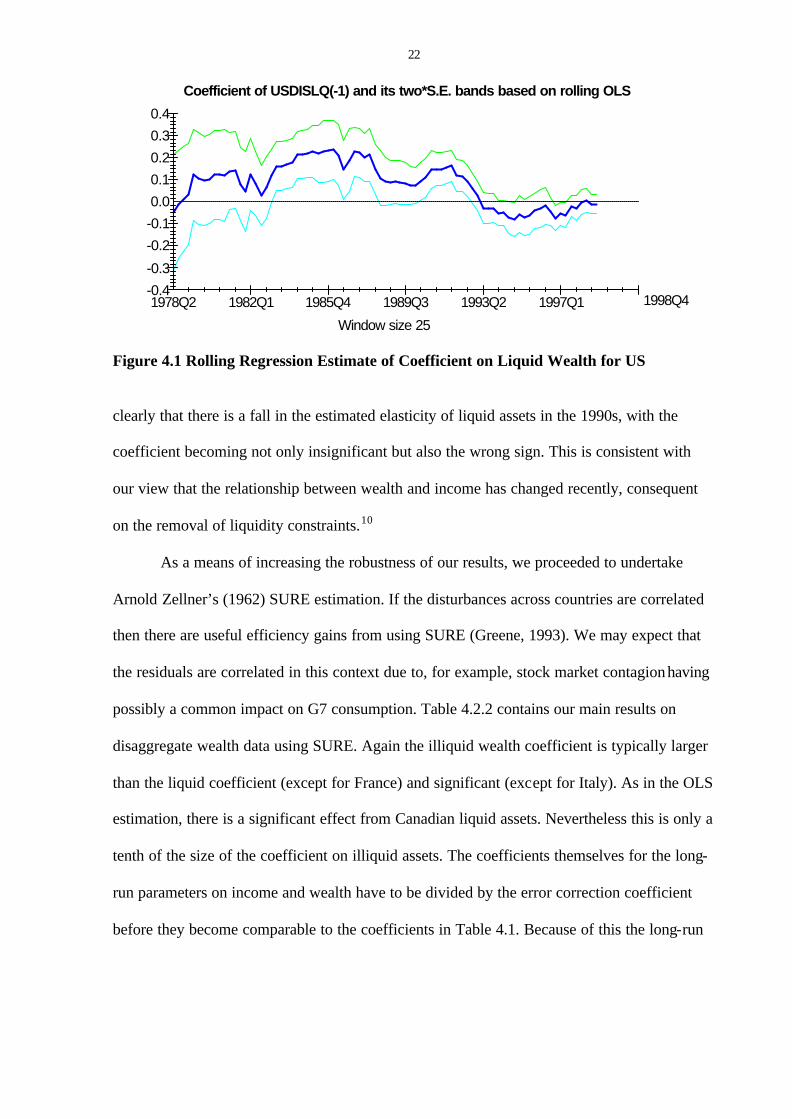
Instability in the parameter estimates is highlighted once again in Figure 4.1, where we

plot the rolling regression estimate of the US coefficient on liquid wealth. We can see quite

22

Coefficient of USDISLQ(-1) and its two*S.E. bands based on rolling OLS

Window size 25

-0.1

-0.2

-0.3

-0.4

0.0

0.1

0.2

0.3

0.4

1978Q2 1982Q1 1985Q4 1989Q3 1993Q2 1997Q1 1998Q4

Figure 4.1 Rolling Regression Estimate of Coefficient on Liquid Wealth for US

clearly that there is a fall in the estimated elasticity of liquid assets in the 1990s, with the

coefficient becoming not only insignificant but also the wrong sign. This is consistent with

our view that the relationship between wealth and income has changed recently, consequent

on the removal of liquidity constraints.10

As a means of increasing the robustness of our results, we proceeded to undertake

Arnold Zellner’s (1962) SURE estimation. If the disturbances across countries are correlated

then there are useful efficiency gains from using SURE (Greene, 1993). We may expect that

the residuals are correlated in this context due to, for example, stock market contagion having

possibly a common impact on G7 consumption. Table 4.2.2 contains our main results on

disaggregate wealth data using SURE. Again the illiquid wealth coefficient is typically larger

than the liquid coefficient (except for France) and significant (except for Italy). As in the OLS

estimation, there is a significant effect from Canadian liquid assets. Nevertheless this is only a

tenth of the size of the coefficient on illiquid assets. The coefficients themselves for the long-

run parameters on income and wealth have to be divided by the error correction coefficient

before they become comparable to the coefficients in Table 4.1. Because of this the long-run

23

Table 4.2.2 SURE Estimation Results with Disaggregate Wealth

US UK Germany France Italy Canada Japan

a1*lnCt-1 -0.169 (3.6)

-0.121 (2.8)

-0.343 (5.6)

-0.135 (4.4)

-0.052 (2.5)

-0.271 (5.1)

-0.117 (2.5)

ß1*lnYt-1 0.158 (3.2)

0.113 (2.9)

0.298 (5.1)

0.143 (3.4)

0.051 (1.5)

0.217 (4.4)

0.104 (2.8)

ß2*lnW[LQ],t -1 -0.004 (1.0)

-0.003 (0.3)

0.015 (1.1)

0.001 (0.0)

0.004 (0.7)

0.008 (2.6)

-0.002 (0.3)

ß3*lnW[ILQ],t -1 0.009 (3.3)

0.011 (3.5)

0.016 (2.3)

0.003 (3.1)

0.002 (2.0)

0.035 (5.9)

0.012 (2.6)

ß4*lnW[MO],t -1 -0.001 (0.1)

2R 0.58 0.65 0.87 0.33 0.66 0.46 0.69

SE 0.005 0.007 0.006 0.006 0.004 0.007 0.007 DW 2.0 1.9 2.1 2.0 2.2 2.3 2.0

Het. ?2(1) 1.8 0.1 0.0 2.6 2.5 0.1 1.0 Notes: Sample period is 1972Q2 to 1998Q4. The wealth terms are ß2*lnW[LQ],t -1 which comprises liquid assets less bank borrowing, ß3*lnW[ILQ],t-1 which is illiquid assets less mortgage debt except for Germany and ß4*lnW[MO],t -1 in the case of Germany is solely mortgage debt. To make our SURE and single equation results comparable it is necessary to divide the long-run coefficients (ßi) by the error correction term (a1). Table 4.2.3 Wald Tests for Equivalence of G7 Coefficients

Income Liquid Wealth Illiquid Wealth Test

Statistic p-value Test

Statistic p-value Test

Statistic p-value

US = UK

-0.003 [.979] -0.002 [.985] 0.040 [.328]

UK= Germany

-0.063 [.621] 0.070 [.546] -0.048 [.264]

Germany = France

0.195 [.096] -0.044 [.604] -0.022 [.349]

France = Italy

-0.084 [.808] 0.075 [.587] 0.007 [.741]

Italy = Canada

-0.181 [.584] -0.045 [.709] 0.097 [.000]

Canada = Japan

0.096 [.149] -0.049 [.457] -0.023 [.527]

Joint Test Statistic ?2(18) = 61.179 p-value = 0.000

coefficients as displayed in Table 4.2.2 should not be compared across countries without a

further transformation.

We went on to conduct formal tests to examine the equivalence of coefficients across

countries. To do so it is necessary to divide the long-run relations by the coefficient on the

10 The estimated coefficient in Figure 4.1 should be divided by the estimated US error correction term in Table

4.2.1 to allow the results to be directly comparable.

24

error correction term. We can then implement joint Wald Tests using n individual results,

which are distributed as a ?2(n) statistics under the null of homogeneity. In particular, the test

undertaken is of equivalence to the US results.

Overall, in Table 4.2.3, the joint test statistic that the US long run coefficients are

equal to those of the other G7 members is strongly rejected. Nevertheless there is quite a

considerable similarity amongst our countries’ coefficients as the large majority of probability

values accept the null of homogeneity of coefficients across countries. Indeed, all liquid

wealth statistics are equivalent across countries which suggest that not only are liquid assets

unimportant as a component of wealth’s impact on consumption but they are equally

unimportant across countries. We then tested the joint hypothesis that the coefficients on

illiquid wealth were homogenous and this was accepted at the 5% significance level with a

test statistic of ?2 (5) = 10.317 [P-value = 0.068], although we excluded Canada since it

appears to be an outlier in this part of the analysis. Additionally we tested whether this group

of countries’ estimated liquid wealth coefficients could be restricted to zero and this was

accepted with a test statistic of ?2 (6) = 2.75687 [P-value = 0.839]. This supports our major

hypothesis.

It is also interesting to test whether there is similar behaviour for the UK and, as it

stands at the moment, the three other G7 countries with a single monetary authority. We do so

by comparing Germany, UK, France and Italy and the results are given in Table 4.2.4.

Table 4.2.4 Wald Tests for Equivalence of European Coefficients

Income Liquid Wealth Illiquid Wealth Test

Statistic p-value Test

Statistic p-value Test

Statistic p-value

UK= Germany

-0.063 [.621] 0.070 [.546] -0.048 [.264]

Germany = France

0.194 [.096] -0.044 [.604] 0.022 [.349]

France = Italy

-0.084 [.808] 0.075 [.587] 0.007 [.741]

Joint Test Statistic ?2(9) = 8.225 p-value = 0.511 Notes: The individual tests examine the equivalence of income, liquid and illiquid wealth coefficients of our four European countries. The estimation method is SURE and sample 1972Q2 to 1998Q4

25

Individually and overall we find that the null of homogeneity is accepted for our four

countries.

We also considered the long-run elasticity of household equity holdings on their own.

We have non-stock market wealth (NSW) and stock market wealth (SW) separated in our

long run specification. The results for the US only are given below:

( )( ) ( ) ( ) ( ) ( ) ( ) ( )2.56.53.27.18.47.27.1

ln*306.0ln*179.0ln031.0ln*151.0ln*731.0ln*138.0095.0ln 21111

=

∆+∆+−−−−=∆ −−−−−

t

YCSWNSWYCC ttttttt

1972Q2 to 1998Q4 2R = 0.59, SE = 0.005, SC-LM ?2 (4)=6.7, Norm ?2 (2) = 4.0, Het ?2 (1) = 1.6

Share ownership on its own is significant in the long-run, with a long-run elasticity of 0.031.

This estimated coefficient is slightly smaller than the coefficient on the combined variable of

share ownership, life assurance and pension minus mortgage debt – which has an elasticity of

0.151. These result support the argument made above that despite their illiquidity, long term

institutional forms of saving may have a strong effect on consumption. 11

4.3 Nested Specification of Disaggregate Wealth

It should be noted that the simple disaggregation approach that we have taken earlier

is not nested within our benchmark equations estimated in Table 4.1. To check that our results

are not the result of a non-nested disaggregation of our long-run relationship, we produce a

disaggregation that has a separate term for illiquid assets and also one plus the ratio of liquid

to illiquid wealth. Algebraically,

( )1,21,11 lnln −−− += ttt WWW ( ))/1(*ln 1,21,11,2 −−− += ttt WWW (11)

This subsequently allows us to embed our nested long-run equation within our dynamic short

run equations.

( ) ktijtitttttt YCWWWYCC −−−−−−− ∆+∆++−−−+=∆ lnln)/1ln(lnlnlnln 1,21,131,2211110 γγβββαα

11 We also considered how sensitive our results were to the definition of bond holdings as illiquid assets. For

Germany it was found that once we defined them as liquid assets the illiquid assets component became

insignificant whereas the liquid component became significant. Italy was also found to have an insignificant

liquid asset component once we change the definition of bonds. For the other countries we do not find the results

26

Table 4.3.1 Consumption Functions with Nested Disaggregate Wealth

US UK Germany France Italy Canada Japan

a1*lnCt-1 -0.151 (3.2)

-0.142 (2.5)

-0.320 (5.1)

-0.115 (3.3)

-0.086 (3.6)

-0.269 (4.6)

-0.136 (2.7)

ß1*lnYt-1 0.787 (8.2)

0.874 (9.4)

0.855 (20.0)

0.939 (5.0)

0.860 (5.5)

0.790 (15.8)

0.874 (17.1)

ß2*lnW2,t -1 0.174 (2.2)

0.118 (2.2)

0.053 (2.1)

0.093 (1.2)

0.193 (3.6)

0.161 (7.9)

0.104 (2.7)

ß3*ln(1+W1,t -1/W2,t -1) 0.276 (1.5)

0.081 (0.4)

0.056 (1.2)

0.079 (0.9)

0.268 (3.3)

0.168 (2.4)

0.007 (0.1)

ß4*ln(WGE3,t -1) 0.013 (0.3)

Wald Test p-values H0:ß 2 = ß3 0.372 0.733 0.950 0.282 0.009 0.911 0.185 H0:ß 1 + ß2 =1, ß 2 = ß3 0.368 0.940 0.004 0.559 0.002 0.410 0.000

2R 0.60 0.66 0.87 0.34 0.69 0.47 0.69 SE 0.005 0.007 0.007 0.007 0.004 0.007 0.007

LM–SC ?2(4) 6.3 5.3 1.5 5.2 5.0 7.9 3.9 Norm ?2(2) 3.4 4.2 3.8 0.5 1.3 1.9 0.1 Het ?2(1) 1.7 0.1 0.1 3.2 3.2 0.1 1.0

Notes: Sample period is 1972Q2 to 1998Q4. The wealth terms are W2,t -1 which is illiquid assets less mortgage debt except for Germany and W1,t -1 comprises liquid assets less bank borrowing. In the case of Germany, we have separate terms for illiquid wealth excluding mortgage debt, liquid wealth and a third disaggregate wealth term ß4*ln(WGE3,t -1) = ß4*ln((1/W1,t -1) + (1/W2,t -1) - mortgage debt/W1,t -1*W2,t -1). We can then test whether the coefficients β2 and β3 are equivalent. Particularly if β3 is

insignificant while β2 is significant, we can be satisfied that a significant coefficient on

illiquid wealth in the above estimates is a reflection of the data and not merely our approach

to disaggregation. We find evidence of a significant effect from illiquid wealth while the

implicit effect from liquid wealth is zero for the US, Japan and the UK, which replicates our

previous results. The German result is more than likely a result of bond holding which are, in

this table, included as illiquid assets. The French results suggest there is no effect from either

component of wealth when separated in a nested specification. Italy and Canada suggest an

important role for both kinds of wealth holdings.

Given our previous results we also test for stability of the regression residuals using

the Andrews’ (1993) SupW and Andrews and Ploberger’s (1994) ExpW tests. For the US we

change by any quantitative and qualitative amount. These results are available included in an earlier version of

27

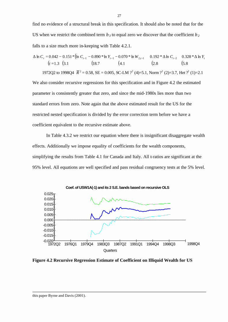
find no evidence of a structural break in this specification. It should also be noted that for the

US when we restrict the combined term β3 to equal zero we discover that the coefficient β2

falls to a size much more in-keeping with Table 4.2.1.

( )( ) ( ) ( ) ( ) ( ) ( )8.58.21.47.181.33.1

ln*328.0ln*192.0ln*070.0ln*890.0ln*151.0042.0ln 21,211

=

∆+∆+−−−=∆ −−−−

t

YCWYCC tttttt

1972Q2 to 1998Q4 2R = 0.58, SE = 0.005, SC-LM ?2 (4)=5.1, Norm ?2 (2)=3.7, Het ?2 (1)=2.1 We also consider recursive regressions for this specification and in Figure 4.2 the estimated

parameter is consistently greater that zero, and since the mid-1980s lies more than two

standard errors from zero. Note again that the above estimated result for the US for the

restricted nested specification is divided by the error correction term before we have a

coefficient equivalent to the recursive estimate above.

In Table 4.3.2 we restrict our equation where there is insignificant disaggregate wealth

effects. Additionally we impose equality of coefficients for the wealth components,

simplifying the results from Table 4.1 for Canada and Italy. All t-ratios are significant at the

95% level. All equations are well specified and pass residual congruency tests at the 5% level.

Coef. of USW1A(-1) and its 2 S.E. bands based on recursive OLS

Quarters

-0.005-0.010-0.015-0.020

0.0000.0050.0100.0150.0200.025

1972Q2 1976Q1 1979Q4 1983Q3 1987Q2 1991Q1 1994Q4 1998Q3 1998Q4

Figure 4.2 Recursive Regression Estimate of Coefficient on Illiquid Wealth for US

this paper Byrne and Davis (2001).

28

Table 4.3.2 Consumption Functions with Nested Disaggregate Wealth

US UK Germany France Italy Canada Japan

a1*lnCt-1 -0.152 (3.2)

-0.134 (3.4)

-0.283 (5.0)

-0.133 (4.2)

-0.060 (2.7)

-0.267 (4.7)

-0.134 (3.6)

ß1*lnYt-1 0.890 (18.7)

0.900 (10.8)

0.865 (19.9)

1.072 (12.8)

0.992 (5.3)

0.790 (15.8)

0.877 (49.9)

ß2*lnW2,t -1 0.070 (2.2)

0.094 (3.4)

0.068 (3.8)

0.023 (3.1)

0.101 (6.5)

ß4*lnWt-1 0.095 (2.2)

0.160 (8.0)

Wald Test p-values H0: ß2 = ß3 0.210 0.927 0.012 0.235 0.555 0.183 0.000

2R 0.60 0.65 0.87 0.34 0.67 0.47 0.69 SE 0.005 0.007 0.007 0.007 0.004 0.007 0.007

LM–SC ?2(4) 6.3 5.6 1.6 5.1 4.6 7.9 3.9 Norm ?2(2) 3.4 4.1 3.8 0.3 1.7 1.9 0.1 Het ?2(1) 1.7 0.1 0.2 3.6 2.2 0.1 1.0

Notes: Sample period is 1972Q2 to 1998Q4. The wealth terms are W2,t -1 which is illiquid assets less mortgage debt except for Germany. In the case of Germany, we have illiquid wealth excluding mortgage debt. Wt-1 comprises net total liquid and illiquid assets. P-values less than 0.05 reject the null for the Wald tests. T-statistics are in parenthesis and where bold are significant at the 95% level.

4.4 Real Non-Property Income

In this section we utilise non-property income (NPYt) in our short and long-run

relationship for consumption instead of real personal disposable income. As noted, real

personal disposable income incorporates some of the components of wealth and hence we

may be including those components twice in our linear regression results. Using data from the

OECD Outlook database NPYt has been constructed by the following definition.

[ ] [ ]( )[ ] tttttttttt

ttt YRHTRPHTRRHEEETWSSSTYHTRPHTRRH

EEET

WSSSNPY −+−−+

= *** (12)

The main components of non-property income are Compensation of Employees

(WSSSt) and Total Transfers Received by Households (TRRHt) minus Direct Taxes (TYHt).

WSSSt is adjusted for the ratio of Total Employment (ETt) to Total Dependent Employment

(EEt) to allow for the income of the self employed. We also remove Total Transfers Paid by

Households (TRPHt) from TRRHt. YRHt is the current receipts of households. We then deflate

29

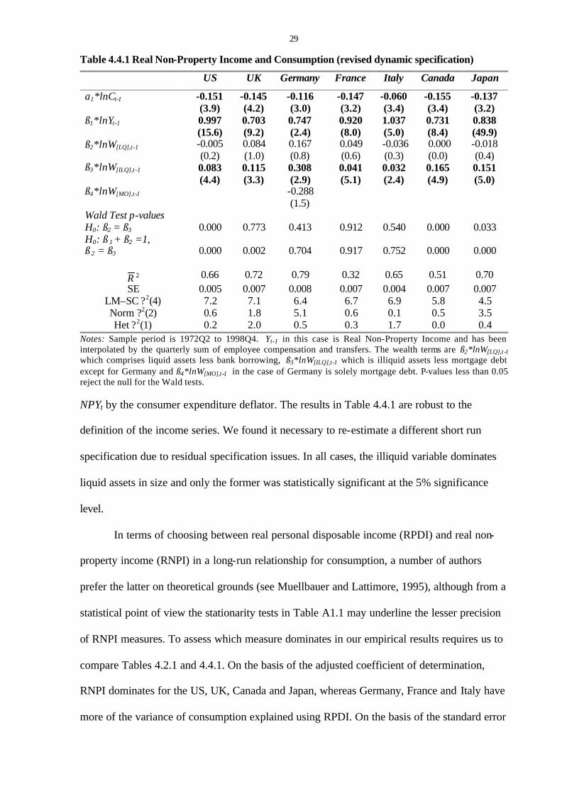
Table 4.4.1 Real Non-Property Income and Consumption (revised dynamic specification)

US UK Germany France Italy Canada Japan

a1*lnCt-1 -0.151 (3.9)

-0.145 (4.2)

-0.116 (3.0)

-0.147 (3.2)

-0.060 (3.4)

-0.155 (3.4)

-0.137 (3.2)

ß1*lnYt-1 0.997 (15.6)

0.703 (9.2)

0.747 (2.4)

0.920 (8.0)

1.037 (5.0)

0.731 (8.4)

0.838 (49.9)

ß2*lnW[LQ],t -1 -0.005 (0.2)

0.084 (1.0)

0.167 (0.8)

0.049 (0.6)

-0.036 (0.3)

0.000 (0.0)

-0.018 (0.4)

ß3*lnW[ILQ],t -1 0.083 (4.4)

0.115 (3.3)

0.308 (2.9)

0.041 (5.1)

0.032 (2.4)

0.165 (4.9)

0.151 (5.0)

ß4*lnW[MO],t -1 -0.288 (1.5)

Wald Test p-values H0: ß2 = ß3 0.000 0.773 0.413 0.912 0.540 0.000 0.033 H0: ß 1 + ß2 =1, ß 2 = ß3

0.000

0.002

0.704

0.917

0.752

0.000

0.000

2R 0.66 0.72 0.79 0.32 0.65 0.51 0.70

SE 0.005 0.007 0.008 0.007 0.004 0.007 0.007 LM–SC ?2(4) 7.2 7.1 6.4 6.7 6.9 5.8 4.5 Norm ?2(2) 0.6 1.8 5.1 0.6 0.1 0.5 3.5 Het ?2(1) 0.2 2.0 0.5 0.3 1.7 0.0 0.4

Notes: Sample period is 1972Q2 to 1998Q4. Yt-1 in this case is Real Non-Property Income and has been interpolated by the quarterly sum of employee compensation and transfers. The wealth terms are ß2*lnW[LQ],t -1 which comprises liquid assets less bank borrowing, ß3*lnW[ILQ],t -1 which is illiquid assets less mortgage debt except for Germany and ß4*lnW[MO],t-1 in the case of Germany is solely mortgage debt. P-values less than 0.05 reject the null for the Wald tests. NPYt by the consumer expenditure deflator. The results in Table 4.4.1 are robust to the

definition of the income series. We found it necessary to re-estimate a different short run

specification due to residual specification issues. In all cases, the illiquid variable dominates

liquid assets in size and only the former was statistically significant at the 5% significance

level.

In terms of choosing between real personal disposable income (RPDI) and real non-

property income (RNPI) in a long-run relationship for consumption, a number of authors

prefer the latter on theoretical grounds (see Muellbauer and Lattimore, 1995), although from a

statistical point of view the stationarity tests in Table A1.1 may underline the lesser precision

of RNPI measures. To assess which measure dominates in our empirical results requires us to

compare Tables 4.2.1 and 4.4.1. On the basis of the adjusted coefficient of determination,

RNPI dominates for the US, UK, Canada and Japan, whereas Germany, France and Italy have

more of the variance of consumption explained using RPDI. On the basis of the standard error

30

of the residuals there is little to differentiate the two approaches. Hence we do not find

sufficient consistent evidence in favour of either measure of income to make a strong

generalisation across countries on the basis of these econometric estimates. Nevertheless the

fact our result regarding the different effects of different measures of wealth stand up across

our two measures of income underlines the robustness of this, our principal result.

4.5 Summary of Results

We seek to bring together the results for our estimated consumption functions with

disaggregated wealth in Table 4.6.1. In this table we only include those terms which are

significant at 90% and above. The summarised results below clearly illustrate that the illiquid

wealth term is dominant in most of the specifications, with the liquid wealth term typically

being insignificant. These results were replicated with SURE analysis in Tables 4.2.2 and

4.3.2. When we use Non-Property Income in our specification, illiquid assets again dominate.

Table 4.6.1 Consumption and Disaggregate Wealth - Summary

US UK Germany France Italy Canada Japan

Total Wealth

0.11 0.13 0.09 0.16 0.1 0.16 0.14

MPC from Total Wealth

0.06 0.02 0.02 0.03 0.02 0.04 0.01

Liquid Insig Insig Insig Insig Insig 0.03 Insig

Illiquid 0.06 0.11 0.05 0.03 Insig 0.14 0.11

DisaggregateWealth

Bonds Illiquid Mort. Insig

Liquid Insig Insig Insig Insig 0.10 0.16 Insig

Illiquid 0.07 0.09 0.07 Insig 0.10 0.16 0.10

Nested Disaggregate

Wealth – Bonds Illiquid Mort. Insig

Liquid Insig Insig Insig Insig Insig Insig Insig

Illiquid 0.08 0.12 0.31 0.04 0.03 0.17 0.15

Disaggregate Wealth –

Bonds Illiquid And NPY Mort. Insig

Notes: “Insig” where the variable coefficient is insignificant at the 10% level. MPC is the Marginal Propensity to Consume out of aggregate wealth and is calculated by multiplying the elasticity of total wealth by the ratio of consumption to wealth over the entire sample period. Mort. is mortgage holdings and is separated out for German and French illiquid assets where it dominates the other components. NPY is Non-Property Income.

31

5. Calibrating the Impact of a Fall in Share Prices

In order to assess the differences between the basic and disaggregated estimates in

current terms, we sought to estimate the likely long term impact on consumption of a 25% fall

in share prices, given the latest balance sheet observation (which varies from 1998 for

Germany and Italy to 2000 for the UK and US). Of course, this is a highly simplified

comparison, which ignores feedback elsewhere from the economy. In order to do this, it is

necessary to estimate the impact of a share price fall not only via directly held equities but

also in terms of the impact on life insurance and pension fund claims. The latter needs to

allow for the fact that only a part of portfolios are typically in the form of equity, and also for

the fact that there are guarantee elements in some of the related financial claims (e.g. defined

benefit pension claims). We used the rough approximation that these effects would entail 50%

of a fall in equity prices affecting life and pension claims in the US, UK and Canada, while in

Germany, France, Italy and Japan it is 25%. Having made this approximation, one can

calculate the effect of a 25% fall in share prices on net financial wealth (for the basic model

calibration set out in Table 4.1) and on net illiquid wealth (in the disaggregated model

calibration set out in Table 4.2.1). The results are reported in Tables 5.1 and 5.2.

Table 5.1 Calibrating the effect of a 25% fall in Share Price – Coefficients and Weights

Coefficient on net wealth (basic

equation)

Coefficient on net illiquid wealth

(disaggregated equation)

Equity/net wealth

Equity/net illiquid wealth

US 0.11 0.06 0.59 0.85 UK 0.13 0.11 0.63 0.79

Germany 0.09 0.05 0.26 0.30 Japan 0.14 0.11 0.21 0.56 France 0.16 0.03 0.60 0.84

Italy 0.10 0.00 (insig) 0.45 0.60 Canada 0.16 0.14 0.93 1.08 Japan 0.14 0.11 0.21 0.56

32

Table 5.2 Calibrating effects of a 25% fall in Share Price – effects on Wealth and Consumption

Effect of 25% equity price fall on net

wealth

Effect of 25% equity price fall on net

illiquid wealth

Effect of 25% equity price fall on consumption

(basic equation)

Effect of 25% equity price fall on consumption

(disaggregated equation) US -0.15 -0.21 -0.017 -0.012 UK -0.16 -0.20 -0.021 -0.022

Germany -0.07 -0.08 -0.006 -0.004 France -0.15 -0.21 -0.024 -0.004

Italy -0.11 -0.15 -0.011 0.000 Canada -0.23 -0.27 -0.037 -0.037 Japan -0.05 -0.14 -0.007 -0.015

As shown in the first two columns of Table 5.1, the coefficient on wealth in the

aggregated equation is higher than that on illiquid wealth in the disaggregated equation in all

cases. In the cases of France and Italy the differences are substantial. As regards the estimated

proportion of wealth which is affected by equity price falls, shown in the third and fourth

columns of Table 5.1, these are often quite sizeable, reflecting the fact that the denominator is

net of loans or mortgages. In Canada, the estimated ratio for equity-related assets to net

financial wealth is close to 1, while illiquid wealth ratios are close to 1 for all countries except

Japan, Germany and Italy. Moving to Table 5.2, the effect of a fall of 25% in share prices is

correspondingly more sizeable for the countries with substantial equity holdings. Finally

multiplying the percent change in wealth by the coefficient gives the change in consumption.

As shown in the last two columns of Table 5.2, the effect is estimated to be largest in Canada,

at 3.7% for both estimates; German results are also consistent at around 0.5%. Elsewhere the

UK and Japan have a higher consumption response with the disaggregated estimate than the

basic equation (2.2% and 1.5% compared to 2.1% and 0.7%, respectively). For other countries

the disaggregated estimate is smaller, at 1.2% for the US (compared to 1.7% for the basic

equation), and 2.4% and 1.0% for France and Italy for their benchmark compared with around

0.4% and 0.0% for the disaggregate equation.

We also calculated the effects of a fall in share prices using the estimates with non-

property income set out in Table 4.6 (not illustrated in the tables above). These in general

gave slightly higher estimates of the effect on consumption of a share price fall. The effect in

33

the US for example is -1.8%, in Canada it is 4.5% and in Japan, 2.1%. For Italy the coefficient

becomes significant with an estimated effect of -0.5%.

6. Conclusion

While they are by no means unequivocal, there is considerable evidence from the

results presented in this paper that the terms on the different sub-components of financial

wealth differ significantly, thus implying that the aggregation of wealth in a typical

consumption function is inappropriate. Furthermore, there is evidence that illiquid wealth

dominates the effect of conventional liquid assets. The different effects from the components

of wealth may be seen as justified in the context of a liberalised financial system, where

consumption is focused on life cycle considerations and lifetime wealth is held increasingly in

securities and institutional investment. In contrast, liquid assets are held largely for

transactions purposes and changes in their volume are less strongly related to consumption.

The robustness of the result to different definitions of liquid and illiquid assets, within a

nested framework and with use of non property income as an income variable strengthens the

results for illiquid wealth.

One implication of the results is that the conventional studies of wealth effects on

consumption are biased as estimates of the likely response of the household sector to falls in

equity prices. This could be of particular relevance for the United States in the short-term, and

also in the longer term for a wider range of countries as financial market liberalisation

proceeds, securities markets develop and portfolios resemble those of the US to a greater

degree. Moreover, the process of ageing, which is already underway, is also driving portfolios

towards holding more illiquid assets.

34

References

Ando, A. and Modigliani, F. (1963). The Life Cycle Hypothesis of Saving: Aggregate

Implications and Tests, American Economic Review, Vol. 103, pp. 55-84.

Andrews, D.W.K. (1993). Tests for Parameter Instability and Structural Change with

Unknown Change Point, Econometrica, Vol. 61, pp. 821-856.

Andrews, D.W.K. and Ploberger, W. (1994). Optimal Tests When a Nuisance Parameter is

Present Only Under the Alternative, Econometrica, Vol. 62, pp. 1383-1414.

Banerjee, A., Dolado, J.J., Galbraith, J.W. and Hendry, D.F. (1993). Cointegration, Error

Correction and the Econometric Analysis of Non-Stationary Data, Oxford University Press,

Oxford.

Bank of England (2000). Economic Models at the Bank of England: September 2000 update,

Bank of England, London.

Berg, L. and Bergstrom, R. (1995). Housing and Financial Wealth, Financial Deregulation

and Consumption – the Swedish Case, Scandinavian Journal of Economics, Vol. 97, pp. 421-

439.

Bonner, X. and Dubois, E. (1995). Peut-on Comprendre la Hausse Imprevue du Taux

D’Epargne des Menages Depuis 1990? Economie et Previsions No. 121. Ministere de

l’Economie, Direction de la Prevision.

Boone, L., Giorno, C. and Richardson, P. (1998). Stock Market Fluctuations and

Consumption Behaviour: Some Recent Evidence, OECD Working Paper No. 208.

Brayton, F. and Tinsley, P. (1996). A Guide to FRB/US – A Macroeconomic Model of the

Federal Reserve Board, Finance and Economics Discussion Paper No. 1996-42, Board of

Governors of the Federal Reserve System.

Brodin, P.A. and Nymoen, R. (1992). Wealth Effects and Exogeneity: The Norwegian

Consumption Function 1966(1)-1989(4), Oxford Bulletin of Economics and Statistics, Vol.

54, pp. 431-49.

35

Byrne, J.P. and Davis, E.P. (2001) Disaggregate Wealth and Aggregate Consumption: An

Investigation of Empirical Relationships for the G7, NIESR Discussion Paper No. 130.

Campbell, J.Y. and Deaton, A. (1989). Why is Consumption So Smooth? Review of Economic

Studies, Vol. 56, pp. 357-373.

Campbell, J.Y. (1996). Understanding Risk and Return, Journal of Political Economy, Vol.

104, pp. 298-345

Campbell, J.Y. and Mankiw, G. (1989). Consumption, Income and Interest Rates,

Reinterpreting the Time Series Evidence, in Blanchard, O. J. and Fischer, S. (eds.), NBER

Macroeconomics Annual, MIT, Cambridge.

Campbell, J.Y. and Mankiw, G. (1991). The Response of Consumption to Income, European

Economic Review, Vol. 35, pp. 723-767.

Carroll, C. (1994). How Does Future Income Affect Current Consumption? Quarterly Journal

of Economics, Vol. 109, pp. 111-147.

Carruth, A., Gibson, H. and Tsakalotos, E. (1999). Are Aggregate Consumption Relationships

Similar Across the European Union? Regional Studies, Vol. 33, pp. 17-26.

Chow, G. and Lin, A. (1971). Best Linear Unbiased Interpolation, Distribution and

Extrapolation of Time Series by Related Series, Review of Economics and Statistics, Vol. 53,

pp. 372-375.

Church, K.B., Smith, P.N. and Wallis, K.F. (1994). Econometric Evaluation of Consumers

Expenditure Equations, Oxford Review of Economic Policy, Vol. 10, pp. 71-85.

Davidson J., Hendry, D., Srba, F. and Yeo, S. (1978). Economic Modelling of the Aggregate

Time Series Relationship Between Consumers’ Expenditure and Income in the United

Kingdom, Economic Journal, Vol. 88, pp. 661-692.

Davis, E.P. (1984). The Consumption Function in Macroeconomic Models: A Comparative

Study, Applied Economics, Vol. 16, pp. 799-838.

36

Davis, E.P. (1995). Financial Fragility in the Early 1990s, What Can Be Learnt from

International Experience? Special Paper No. 76, LSE Financial Markets Group.

Davis, E.P. (1999). Institutionalisation and EMU: Implications for European Financial

Markets, International Finance, Vol. 2, pp. 33-61.

Davis, E P. and Steil, B. (2001). Institutional Investors, MIT Press.

Davis, M .A. and Palumbo, M.G. (2001). A Primer on the Economics and Time Series

Econometrics of Wealth Effects, Finance and Economics Discussion Paper, Federal Reserve

Board Washington.

Deaton, A. (1992). Understanding Consumption, Oxford University Press, Oxford.

De Bondt, G.J. (1999). Credit Channels in Europe – a Cross Country Investigation, Banca

Nazionale del Lavoro Quarterly Review, Vol. 52, pp. 295-326.

Dynan, K., Skinner, J. and Zeldes, S.P. (2000). Do the Rich Save More? NBER Working

Paper No. 7906.

Federal Reserve Bank of Kansas City (1999). New Challenges for Monetary Policy, Jackson

Hole, Wyoming. http://www.kc.frb.org/Publicat/sympos/1999/sym99prg.htm

Gali, J. (1990). Finite Horizons, Life-Cycle Savings and Time Series Evidence on

Consumption, Journal of Monetary Economics, Vol. 26, pp. 433-52.

Gertler, M., Goodfriend, M. , Issing, O. and Spaventa, L. (1998). Asset Prices and Monetary

Policy: Four Views, BIS/CEPR, Basle.

Grunspan, T. and Sicsic, P. (1997). Les Effets de Richesse, Conseil National du Credit et du

Titre, Rapport Annuel, pp. 187-192.

Hansen, B.E. (2000). Testing for Structural Change in Conditional Models, Journal of

Econometrics, Vol. 97, pp. 93-115.

Hendry, D. and von Ungern Sternberg, T. (1981). Liquidity and Inflation Effects on

Consumers’ Expenditure, in Deaton, A. (ed.), Essays in the Theory and Measurement of

Consumer Behaviour, Cambridge University Press, Cambridge.

37

IMF (2000). World Economic Outlook, Spring, International Monetary Fund, Washington

DC.

Kennedy, N. and Anderson, P. (1994). Household Saving and Real Housing Prices: An

International Perspective, B.I.S. Working Paper No. 20.

Lattimore, R. (1993). Consumption and Saving in Australia, Oxford D. Phil thesis.

Lettau, M., Ludvigson, S. and Barczi, N. (2001). A Primer on the Economics and Times

Series Econometrics of Wealth Effects, mimeo, Federal Reserve Bank of New York.

Lettau, M. and Ludvigson, S. (2001a). Consumption, Aggregate Wealth and Expected Stock

Returns, Journal of Finance, Vol. 56, pp. 815-849.

Lettau, M. and Ludvigson, S. (2001b). Resurrecting the, (C)CAPM: A Cross-Sectional Test

When Risk Premia are Time-varying, Journal of Political Economy forthcoming.

Lettau, M. and Ludvigson, S. (2001c). Time varying risk premia and the cost of capital: An

alternative implication of the Q Theory of Investment, Unpublished paper, Federal Reserve

Bank of New York.

Lettau, M. and Ludvigson, S. (2001d). Understanding Trend and Cycle in Asset Values,

mimeo, Federal Reserve Bank of New York.

Ludvigson, S. and Steindel, C. (1999). How Important is the Stock Market Effect on

Consumption? Economic Policy Review, Federal Reserve Bank of New York, July.

Maddala, G.S. and Kim, I-M. (1998). Unit Roots, Cointegration and Structural Change,

Cambridge University Press, Cambridge.

Muellbauer, J. and Lattimore, R. (1995). The Consumption Function, In M.H. Pesaran and M.

Wickens, (eds.), Handbook of Applied Econometrics: Macroeconomics, Blackwell, Oxford.

Muellbauer, J. and Murphy, A. (1994). Explaining Regional Consumption in the UK, mimeo,

Nuffield College, Oxford.

Murata, K. (1994). The Consumption Function in Japan, Oxford M. Phil. Thesis.

38

Nelson, C.R. (1987). A Reappraisal of Recent Tests of the Permanent Income Hypothesis,

Journal of Political Economy, Vol. 95, pp. 641-646.

Ogawa, K., Kitasaka, S., Yamaoka, H. and Iwata, Y. (1996). An Empirical Re-evaluation of

Wealth Effect in Japanese Household Behaviour, Japan and the World Economy, Vol. 8, pp.

423-442.

Pesaran, M.H. and Evans, R.A. (1984). Inflation, Capital Gains and UK Personal Savings:

1953-57, Economic Journal, Vol. 94, pp. 237-57.

Pesaran, M.H. and Pesaran, B. (1997). Microfit 4.0, Oxford University Press, Oxford.

Pesaran, M.H., Shin, Y. and Smith, R.P. (1999). Pooled Mean Group Estimation of Dynamic

Heterogeneous Panels, Journal of the American Statistical Association, Vol. 94, pp. 621-634

Poterba, J. (2000). Stock Market Wealth and Consumption, Journal of Economic

Perspectives, Vol. 14, pp. 99-118.

Poterba, J. and Samwick, A. (1995). Stock Ownership Patterns, Stock Market Fluctuations

and Consumption, Brookings Papers on Economic Activity 2, pp. 295-357.

Starr-McCluer, M. (1999). Stock Market Wealth and Consumer Spending, mimeo, Federal

Reserve Board of Governors.

Stock, J.H. and Watson, M.W. (2001). Forecasting Output and Inflation: The Role of Asset

Prices, http://ksghome.harvard.edu/~.JStock.Academic.Ksg/papers.htm

Townend, J. C. (1978). Modelling UK Consumption, Bank of England Quarterly Bulletin.

Woodford, M. (1994). Non-Standard Indicators for Monetary Policy, in N. Gregory Mankiw,

(ed.), Monetary Policy, University of Chicago Press, Chicago, pp. 99-115.

Zellner, A. (1962). An Efficient Method of Estimating Seemingly Unrelated Regressions and

Tests for Aggregation Bias, Journal of American Statistical Association, Vol. 57, pp. 348-68.

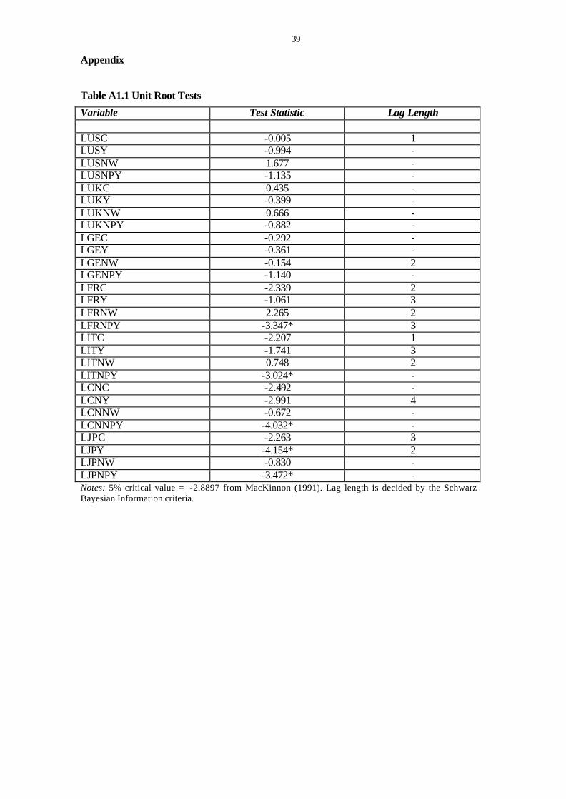
39

Appendix

Table A1.1 Unit Root Tests

Variable Test Statistic Lag Length

LUSC -0.005 1 LUSY -0.994 - LUSNW 1.677 - LUSNPY -1.135 - LUKC 0.435 - LUKY -0.399 - LUKNW 0.666 - LUKNPY -0.882 - LGEC -0.292 - LGEY -0.361 - LGENW -0.154 2 LGENPY -1.140 - LFRC -2.339 2 LFRY -1.061 3 LFRNW 2.265 2 LFRNPY -3.347* 3 LITC -2.207 1 LITY -1.741 3 LITNW 0.748 2 LITNPY -3.024* - LCNC -2.492 - LCNY -2.991 4 LCNNW -0.672 - LCNNPY -4.032* - LJPC -2.263 3 LJPY -4.154* 2 LJPNW -0.830 - LJPNPY -3.472* - Notes: 5% critical value = -2.8897 from MacKinnon (1991). Lag length is decided by the Schwarz Bayesian Information criteria.

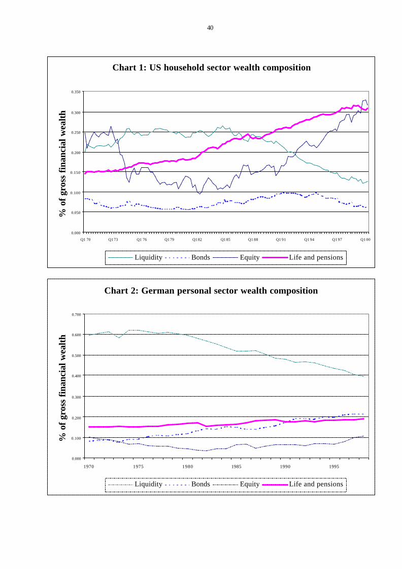
40

Chart 1: US household sector wealth composition

0.000

0.050

0.100

0.150

0.200

0.250

0.300

0.350

Q1 70 Q1 73 Q1 76 Q1 79 Q1 82 Q1 85 Q1 88 Q1 91 Q1 94 Q1 97 Q1 00

% o

f gro

ss fi

nanc

ial w

ealth

Liquidity Bonds Equity Life and pensions

Chart 2: German personal sector wealth composition

0.000

0.100

0.200

0.300

0.400

0.500

0.600

0.700

1970 1975 1980 1985 1990 1995

% o

f gro

ss fi

nanc

ial w

ealth

Liquidity Bonds Equity Life and pensions

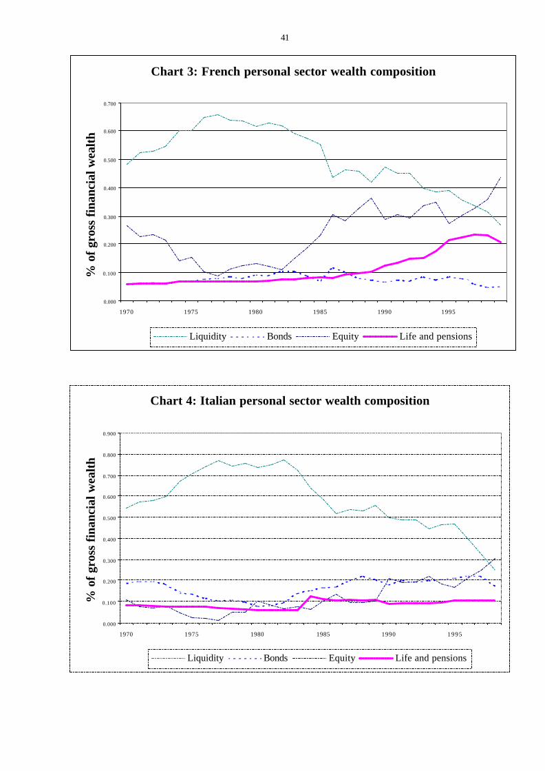
41

Chart 3: French personal sector wealth composition

0.000

0.100

0.200

0.300

0.400

0.500

0.600

0.700

1970 1975 1980 1985 1990 1995

% o

f gro

ss fi

nanc

ial w

ealth

Liquidity Bonds Equity Life and pensions

Chart 4: Italian personal sector wealth composition

0.000

0.100

0.200

0.300

0.400

0.500

0.600

0.700

0.800

0.900

1970 1975 1980 1985 1990 1995

% o

f gro

ss fi

nanc

ial w

ealth

Liquidity Bonds Equity Life and pensions

42

Chart 5: UK personal sector wealth composition

0.000

0.100

0.200

0.300

0.400

0.500

0.600

Q1 70 Q1 73 Q1 76 Q1 79 Q1 82 Q1 85 Q1 88 Q1 91 Q1 94 Q1 97 Q1 00

% o

f gro

ss fi

nanc

ial w

ealth

Liquidity Bonds Equity Life and pensions

Chart 6: Canadian household sector wealth composition

0.00

0.05

0.10

0.15

0.20

0.25

0.30

0.35

0.40

0.45

1970Q1 1973Q1 1976Q1 1979Q1 1982Q1 1985Q1 1988Q1 1991Q1 1994Q1 1997Q1

% o

f gro

ss fi

nanc

ial w

ealth

Liquidity Bonds Equity Life and pensions

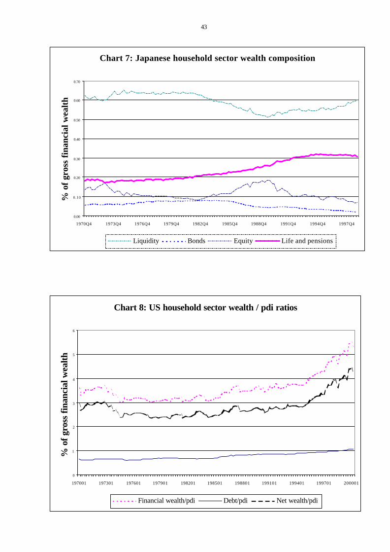
43

Chart 8: US household sector wealth / pdi ratios

0

1

2

3

4

5

6

197001 197301 197601 197901 198201 198501 198801 199101 199401 199701 200001

% o

f gro

ss fi

nanc

ial w

ealth

Financial wealth/pdi Debt/pdi Net wealth/pdi

Chart 7: Japanese household sector wealth composition

0.00

0.10

0.20

0.30

0.40

0.50

0.60

0.70

1970Q4 1973Q4 1976Q4 1979Q4 1982Q4 1985Q4 1988Q4 1991Q4 1994Q4 1997Q4

% o

f gr

oss

fina

ncia

l wea

lth

Liquidity Bonds Equity Life and pensions

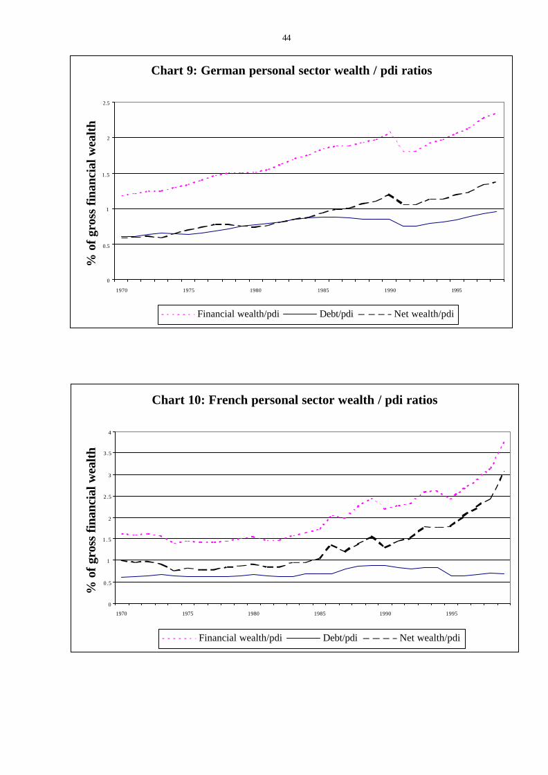
44

Chart 10: French personal sector wealth / pdi ratios

0

0.5

1

1 . 5

2

2.5

3

3.5

4

1970 1975 1980 1985 1990 1995

% o

f gro

ss fi

nanc

ial w

ealth

Financial wealth/pdi Debt/pdi Net wealth/pdi

Chart 9: German personal sector wealth / pdi ratios

0

0.5

1

1.5

2

2.5

1970 1975 1980 1985 1990 1995

% o

f gro

ss fi

nanc

ial w

ealth

Financial wealth/pdi Debt/pdi Net wealth/pdi

45

Chart 11: Italian personal sector wealth / pdi ratios

0

0.5

1

1 . 5

2

2.5

3

3.5

1970 1975 1980 1985 1990 1995

% o

f gro

ss fi

nanc

ial w

ealt

h

Financial wealth/pdi Debt/pdi Net wealth/pdi

Chart 12: UK personal sector wealth / pdi ratios

0

1

2

3

4

5

6

Q1 70 Q1 73 Q1 76 Q1 79 Q1 82 Q1 85 Q1 88 Q1 91 Q1 94 Q1 97 Q1 00

% o

f gro

ss fi

nanc

ial w

ealt

h

Financial wealth/pdi Debt/pdi Net wealth/pdi

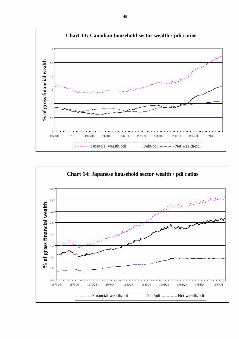
46

Chart 14: Japanese household sector wealth / pdi ratios

0.00

0.50

1.00

1.50

2.00

2.50

3.00

3.50

4.00

1970Q4 1973Q4 1976Q4 1979Q4 1982Q4 1985Q4 1988Q4 1991Q4 1994Q4 1997Q4

% o

f gro

ss fi

nanc

ial w

ealth

Financial wealth/pdi Debt/pdi Net wealth/pdi

Chart 13: Canadian household sector wealth / pdi ratios

0

0 . 5

1

1 . 5

2

2 . 5

3

1970Q1 1973Q1 1976Q1 1979Q1 1982Q1 1985Q1 1988Q1 1991Q1 1994Q1 1997Q1

% o

f gro

ss fi

nanc

ial w

ealt

h

Financial wealth/pdi Debt/pdi Net wealth/pdi