NASATechnical NASA-TP-25_8_98C_00035S8Paper2518

October 1985

A Method for DeterminingAcoustic-Liner Admittancein Ducts With Sheared Flowin Two Cross-Sectional

Directions

Willie R. Watson

fil/A

https://ntrs.nasa.gov/search.jsp?R=19860003588 2018-07-09T06:02:41+00:00Z

NASA 3 1176 01358 4876 _

TechnicalPaper2518

1985

A Method for DeterminingAcoustic-Liner Admittancein Ducts With Sheared Flowin Two Cross-SectionalDirections

Willie R. Watson

Langley ResearchCenterHampton, Virginia

National Aeronauhcsand Space Administration

Scientific and TechnicalInformation Branch

i

ii

SYMBOLS

[A] stiffnessmatricesfor discretizedfinite-elementregion

[A],[B] upper triangular matrices

[Aq],[Bq] element stiffness and mass matrix, respectively, for element q

a width of rectangular element

aI,j'al,J'complex matrix coefficients

bI,j'bI,j J

[B] mass matrices for discretized finite-element region

b height of rectangular element

c ambient speed of sound

E residual error

F acoustic pressure function for impedance tube

F£,M£ respective value of pressure eigenfunction and mean-flow profile at node £

fl,f2 one-dimensional shape functions

H,L height and width, respectively, of impedance tube

K free-space wave number

K dimensional axial propagation constantx

Kx dimensionless axial propagation constant

£ node number

M mean-flow profile

M centerline Mach numbero

m cross-mode order

n integer I or 2 denoting particle velocity or particle displacement,respectively

NY,NZ total number of elements in y- and z-direction, respectively

N£ two-dimensional shape function

SPL sound pressure level

P acoustic pressure

iii

t time

x,y,z Cartesian coordinates

xi,Yi,ZI Cartesian coordinate values at node I

81,B2,B3,84 acoustic admittances of wall lining

8m acoustic admittance

n,_ dimensionless local coordinate system for element

eigenvalue for cross-mode order, mm

{_} global vector of unknowns

{_q} vector of unknown nodal values for element q

angular frequency

Subscripts:

I,J,m integers

Superscript:

tr vector transpose

Mathematical notation:

[ ] matrix

{} vector

det I I determinate of matrix

iv

INTRODUCTION

The reduction of high intensity noise radiating from jet engine aircraft hasbeen the subject of continuous investigation for the past two decades. At the pres-ent time, mathematical models for predicting the noise radiated from these enginesare well developed (ref. 1). However, these prediction models cannot be used withconfidence to predict noise levels radiating from a jet engine in a realistic flowenvironment. Before this confidence can be achieved, it is necessary to obtain accu-rate determinations of the physical parameters, which are input to the predictionmodels. The two critical input parameters are the source input and the admittance ofthe sound-absorbing material. This paper addresses the determination of the latterof these two important input parameters.

Experiments with sound-absorbing materials in the presence of flow indicatesignificant differences in acoustic performance as the mean-flow Mach number is var-ied (ref. 2). This necessitates that sound-absorbing properties of acoustic materi-als be evaluated experimentally in flow. To account for the effects of the meanflow, a test sample of the acoustic-lining material is normally installed in agrazing-flow impedance tube with a controlled aeroacoustic environment. In such agrazing-flow impedance tube, usually rectangular in cross section, the acoustic mate-rial is aligned so that the sound and mean-flow graze over its surface in a mannersimulating an engine environment. In principle, the acoustic admittance can bedetermined by direct measurements of normal particle velocity and pressure sinceacoustic admittance is the ratio of normal particle velocity to pressure at the wallsurface. However, measurements of normal velocity in the presence of grazing floware not reliable. Instead, an indirect measurement approach (ref. 3) has been usedwhich makes use of changes in the wave field caused by the introduction of the testsample in the hard-walled impedance tube. These measurements are then used to calcu-late the acoustic admittance.

Analytical methods for directly determining acoustic admittances from pressuremeasurements taken in a grazing-flow impedance tube have progressed slowly.Armstrong, Beckemeyer, and Olsen (ref. 2) developed a method that is restricted tothin boundary-layer flows with shear in one cross-sectional direction of the tube.This method used an asymptotic expansion to derive a boundary condition that isapplicable at the boundaries of the uniform region in which an exact solution ispossible. Mungur and Gladwell (ref. 3) developed a method that is applicable to moregeneral boundary layers, including cases where the boundary layer spans the _ntiretube. This method is based upon a Runge-Kutta integration across the boundary layerand is restricted to grazing flows with shear in a single cross-sectional direction.Watson (ref. 4) developed a finite-element method for calculating acoustic admit-tances from acoustic pressure data in a grazing-flow impedance tube with one-dimensional shear.

The methods presented in references 2, 3, and 4 are restricted to infinitelylong test samples with mean shear in a single cross-sectional direction of an imped-ance tube. However, grazing-flow duct facilities commonly employ ducts with a rela-tively small rectangular cross section in which the grazing flow possesses shear inboth cross-sectional directions of the impedance tube, such as the flow impedancetest laboratory at the Langley Research Center. Thus, the present effort was moti-

vated by the need to account for the more realistic flow environment with shear inboth cross-sectional directions of laboratory flow-impedance tubes.

This paper describes a method for determining the admittance of an acousticmaterial in a grazing-flow impedance tube in which the grazing flow is assumed topossess shear in both cross-sectional directions. The analysis is restricted tosound fields which are dominated by a single propagating mode. The method is devel-oped explicitly for rectangular ducts, although the approach is applicable to otherduct geometries as well. Experimental input data needed include an estimate of theaxial propagation constant, the two-dimensional mean-flow profile, and acoustic pres-sures parallel to the treated wall of the impedance tube. From these experimentallydetermined characteristics of the aeroacoustic field, the admittance can be calcu-lated. In this paper, the unknown admittance value is obtained by solving an eigen-value problem. This eigenvalue problem results from the application of the finite-element method to the partial differential equation and boundary conditions governingthe acoustic field.

The paper is divided into four sections. The first section presents the gov-erning partial differential equation and boundary conditions. In the second section,a finite-element scheme is applied to obtain the solution to this problem. Thefinite-element method leads to an eigenvalue problem which requires a special schemeto obtain its solution. This eigenvalue solution scheme is developed in the thirdsection of this paper. Finally, the paper closes with a discussion of someapplications.

MATHEMATICAL FORMULATION

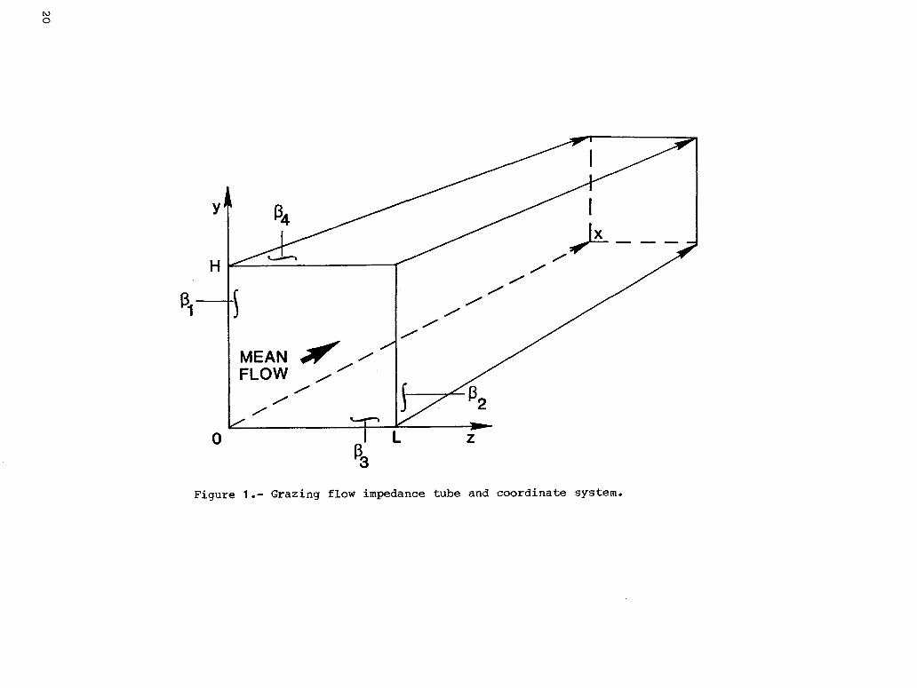
Figure 1 depicts the cross-sectional geometry of the grazing-flow impedance-tubetest section and its coordinate system. All four walls of the tube are lined withacoustic treatment and are assumed infinite in extent. The mathematical developmentassumes that the mean flow in the test section is axial and fully developed, so thatflow gradients exist only in the y- and z-direction.

The solution of the wave equation for harmonic time dependence in the presenceof shear can be written in the form:

-i(KxX- t)P(X,y,z,t) = F(y,z)e (I)

where _ is the axial propagation constant. The following elliptic partial differ-ential equation for the pressure function F(y,z) is obtained (refo 5):

Ecyz(i xl[Fyy+Fzz]+2£x[MyFy.MzFz]

where

In equation (2), the function M = M(y,z) is the mean flow profile, Kx is thedimensionless axial propagation constant in the impedance tube, and K is the free-space wave number (e/C)o

The physical boundary conditions associated with equation (2) require eithercontinuity of particle displacement or continuity of normal particle velocity alongthe four walls of the impedance tube (ref. I). These boundary conditions can beexpressed in the form:

Fz(y,0) = -iK8111 - M(y,0)Kx]n F(y,0) (3)

Fz(y,L) = iK8211 - M(y,L)Kx] n F(y,L) (4)

Fy(0,z) = -iK8311 - M(0,Z)Kx]n F(0,z) (5)

Fy(H,z) = iK8411 - M(H,Z)Kx]n F(H,z) (6)

where 81, 82, 83, and 84 are the specific acoustic admittances of the acousti-cally lined walls. (See fig. I.) Continuity of acoustic particle displacement atthe lined walls are obtained by setting the integer n to 2, whereas continuity ofacoustic particle velocity is obtained by setting n to I. It is instructive tonote that realistic mean-flow profiles satisfy the condition of no slip at the bound-aries rendering a zero mean flow there. Thus, for realistic mean flows, both formsof the boundary condition coalesce to the same expression at each wall. However,since some unrealistic mean velocity profiles are used in this paper in order tocheck with former works, n will be carried throughout the analysis as a parameter.

Equations (2) through (6) constitute a boundary value problem for the acoustic

pressure function F(y,z). The axial propagation constant Kx, free-space wave num-ber K, mean-flow profile M(y,z), boundary condition order n, and wall-lining

admittances 81, 82, and 83 are assumed specified and are treated as known. Thehomogeneity of equations (2) through (6) then allows the determination of the func-

tion F(y,z) and unknown acoustic admittance 84.

Upon obtaining the value of the necessary parameters, the boundary value problemposed by equations (2) through (6) can be solved to obtain the function F(y,z) and

unknown admittance 84. However, equation (2) is a partial differential equationwith variable coefficients and its solution can be put in terms of known functionsonly for some special cases of the two-dimensional sheared flow, M(y,z). However,these cases cannot generally be achieved in the laboratory and are not useful forgeneral application. Thus, the admittance and pressure eigenfunction F(y,z) must

be determined numerically for mean flows of practical interest. A numerical methodfor finding these solutions is described in the following section.

NUMERICAL SOLUTION TECHNIQUE

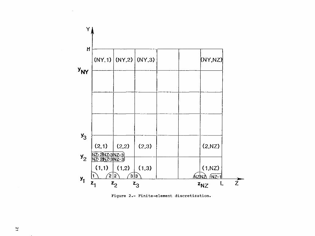
Two principal decisions in the adoption of a numerical technique were the use ofa Galerkin finite-element method and use of linear shape functions to approximate thepressure function and mean-flow profile. The discretization mesh is shown in fig-ure 2. The cross-sectional area of the impedance tube has been divided into NYand NZ elements in the y- and z-direction, respectively. A typical element (I,J)

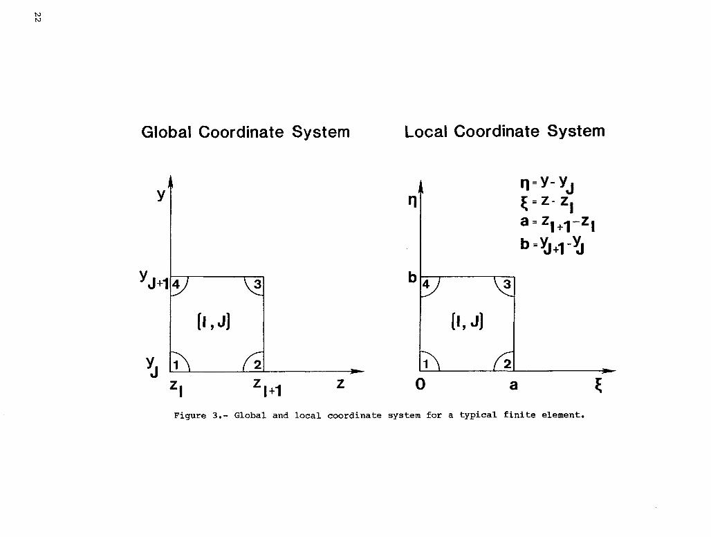
has length (zi+I - zI) and (YJ+I - YJ) in the z- and y-direction, respectively. Inorder to generalize and also simplify the formulation, it is convenient to define alocal coordinate system for each element. This local coordinate system, shown infigure 3, also facilitates the integration which is required to obtain the elementequation.

In order to develop the element equations for a typical element (I,J), the pres-sure function F(_,_) and mean-flow profile M(n,_) are expressed in a form whichensures continuity of these functions both within the element and also along lineswhich are common between any two of the elements. In a typical element, these func-tions are approximated by linear interpolation functions of the form

F(n,_) = N£(n,_) F£ (£ = 1 to 4) (7)

M(_,_) = N£(_,_) M£ (£ = I to 4) (8)

in which repeated subscripts are to be summed over, F and M are the values ofthe functions F(_,_) and M(n,_) at node £ of the£element,£and

NI = f1(_'b) f1(_'a) (9)

N2 = f1(_'b) f2(_,a) (10)

N3 = f2(n,b) f2(_,a) (11)

N4 = f2(n,b) fl(_,a) (12)

f1(n'b) = 1 - _--b (13)

4

f2(n,b) = n_-b (14)

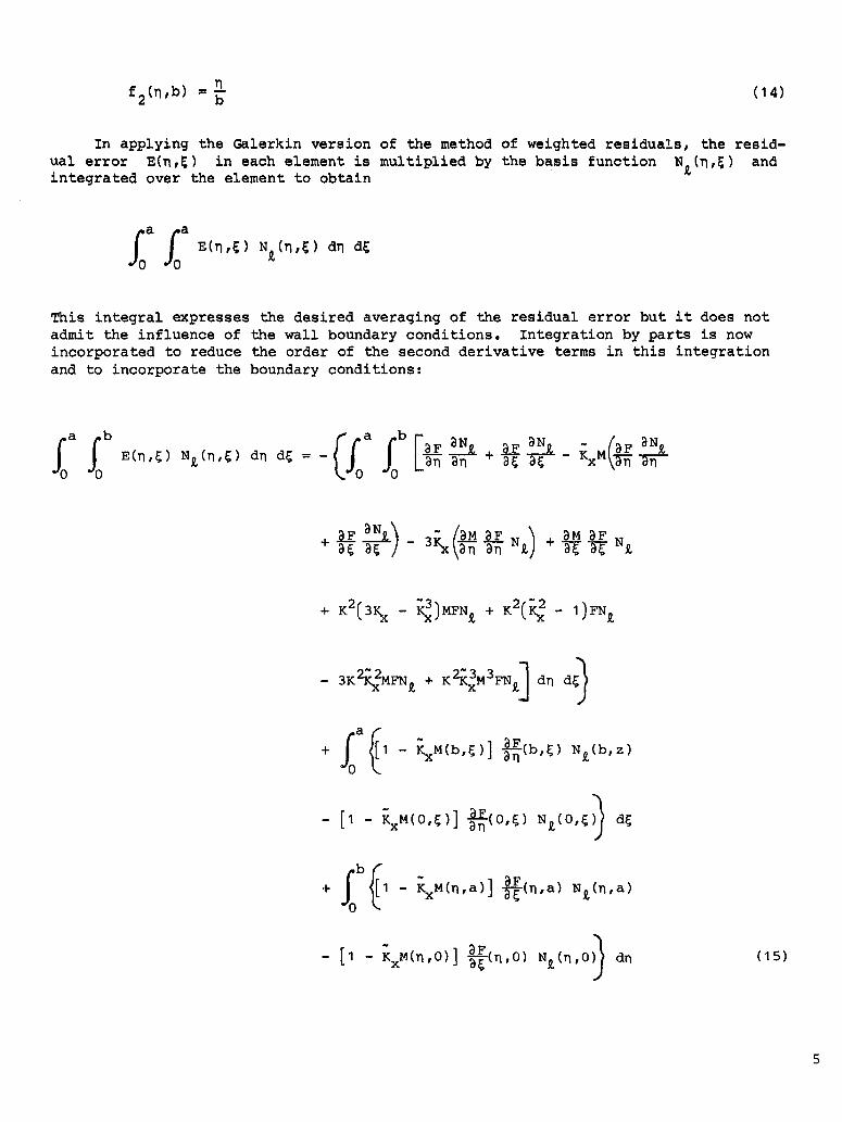
In applying the Galerkinversionof the method of weightedresiduals,the resid-

ual error E(n,_) in each elementis multipliedby the basis function N£(_,_) andintegratedover the elementto obtain

foa foa E(n,_)NA(n,_)dn dE

This integralexpressesthe desired averagingof the residualerror but it does notadmit the influenceof the wall boundaryconditions. Integrationby parts is nowincorporatedto reduce the order of the second derivativeterms in this integrationand to incorporatethe boundaryconditions:

a ob (f0a _0b [T_x" \'a-ffnag-

a(+fo , - _.x>,<b,_>]_<b,_>N_<b,:>

- [i - _,..(o,_)]£(o,_),_<o,_>}_

+ SO I - KxM(n,a)]_(n,a) N£(_,a)

- [i 7_x.(,_,o)] _F )1- _(a,0) N£(n,0 dn (15))

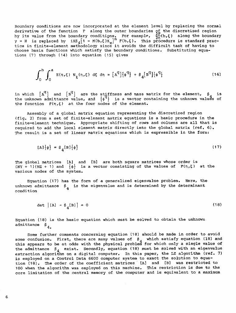
Boundary conditions are now incorporated at the element level by replacing the normalderivative of the function F along the outer boundaries Qf the discretized regionby its value from the boundary conditions. For example, _-F-F(b,_)along the boundary~ n _y = H is replaced by iK8411 - M(b,_)Kx] F(b,_). This procedure is standard prac-tice in finite-element methodology since it avoids the difficult task of having tochoose basis functions which satisfy the boundary conditions. Substituting equa-tions (7) through (14) into equation (15) gives

b a

in which [Aq] and [Bq] are the stiffness and mass matrix for the element, 8- is

the unknown admittance value, and {#q} is a vector containing the unknown values ofthe function F(D,_) at the four nodes of the element.

Assembly of a global matrix equation representing the discretized region(fig. 2) from a set of finite-element matrix equations is a basic procedure in thefinite-element technique. Appropriate shifting of rows and columns are all that isrequired to add the local element matrix directly into the global matrix (ref. 6).The result is a set of linear matrix equations which is expressible in the form:

EAI{ }=84tB { } (17)

The global matrices [A] and [B] are both square matrices whose order is(NY + I)(NZ + 1) and {#} is a vector consisting of the values of F(n,_) at thevarious nodes of the system.

Equation (17) has the form of a generalized eigenvalue problem. Here, the

unknown admittance 84 is the eigenvalue and is determined by the determinantcondition

det I[A] - 84[B]I = 0 (18)

Equation (18) is the basic equation which must be solved to obtain the unknownadmittance 84.

Some further comments concerning equation (18) should be made in order to avoid

some confusion. First, there are many values of 84 which satisfy equation (18) andthis appears to be at odds with the physical problem for which only a single value of

the admittance 84 exist. Secondly, equation (18) must be solved with an eigenvalueextraction algorithm on a digital computer. In this paper, the LZ algorithm (ref. 7)is employed on a Control Data 6600 computer system to exact the solution to equa-tion (18). The order of the coefficient matrices [A] and [B] was restricted to100 when the algorithm was employed on this machine. This restriction is due to thecore limitation of the central memory of the computer and is equivalent to a maximum

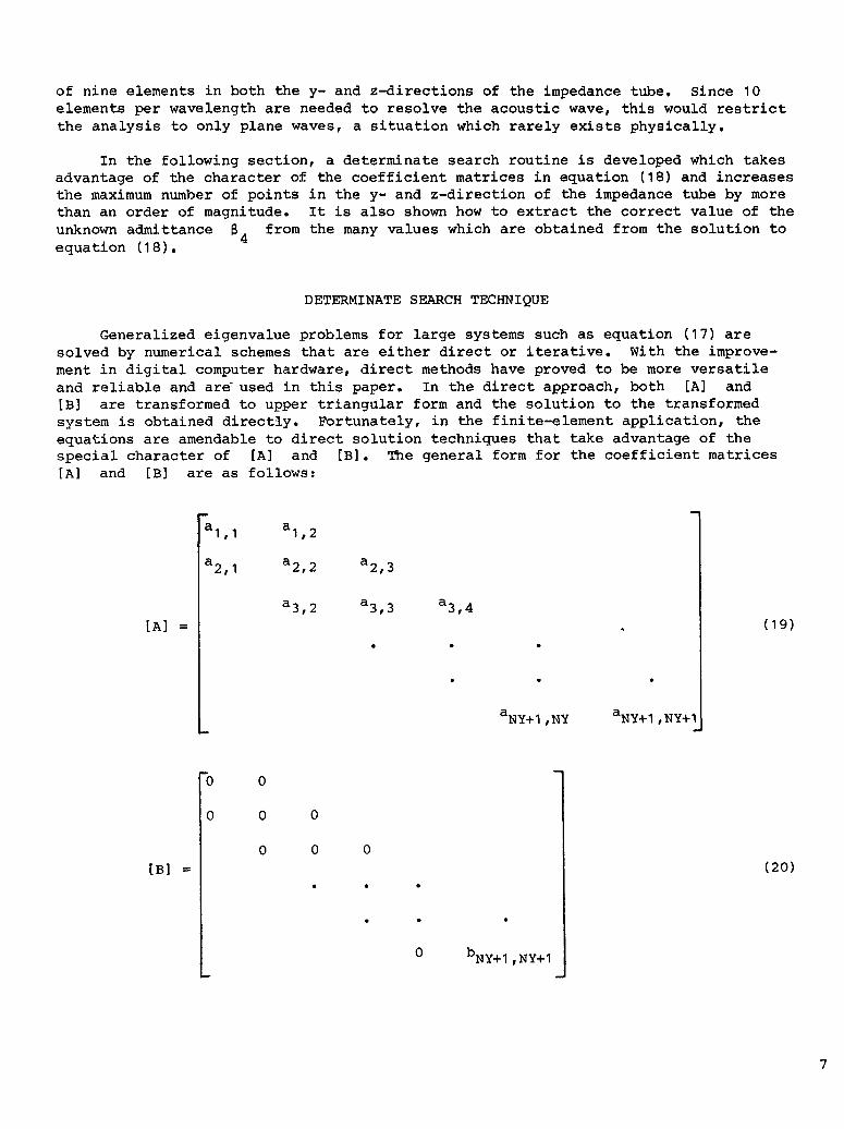
of nine elements in both the y- and z-directions of the impedance tube. Since 10elements per wavelength are needed to resolve the acoustic wave, this would restrictthe analysis to only plane waves, a situation which rarely exists physically•

In the following section, a determinate search routine is developed which takesadvantage of the character of the coefficient matrices in equation (18) and increasesthe maximum number of points in the y- and z-direction of the impedance tube by morethan an order of magnitude• It is also shown how to extract the correct value of the

unknown admittance 84 from the many values which are obtained from the solution toequation (18)•

DETERMINATE SEARCH TECHNIQUE

Generalized eigenvalue problems for large systems such as equation (17) aresolved by numerical schemes that are either direct or iterative. With the improve-ment in digital computer hardware, direct methods have proved to be more versatileand reliable and are used in this paper• In the direct approach, both [A] and[B] are transformed to upper triangular form and the solution to the transformedsystem is obtained directly. Fortunately, in the finite-element application, theequations are amendable to direct solution techniques that take advantage of thespecial character of [A] and [B]. The general form for the coefficient matrices[A] and [B] are as follows:

Jm

al 1 al, ,2

a2,1 a2,2 a2,3

a3,2 a3,3 a3,4[A] = , (19)

I aNY+I ,NY aNY+I ,NY+_

I

"0 0

0 0 0

0 0 0

[B] = (20)

0 bNY+I ,NY+I

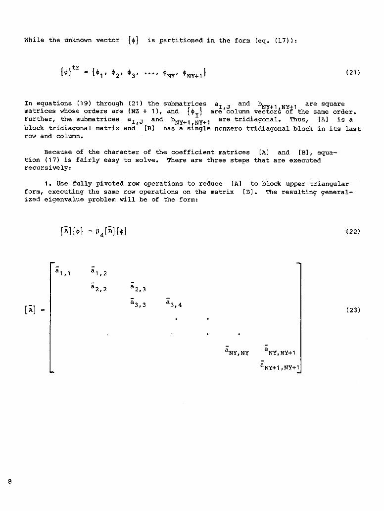
While the unknown vector {_} is partitioned in the form (eq. (17)):

{_}tr = {_1' _2' _3' •'•' #NY' @NY+I} (21)

In equations (19) through (21) the submatrices ai,J and b_v_ _v_1 are squarematrices whose orders are (NZ + I), and {_i} are column ve_t_o£_"6f'thesame order•Further, the submatrices aI,J and bNY+1,NY+I are tridiagonal. Thus, [A] is ablock tridiagonal matrix and [B] has a single nonzero tridiagonal block in its lastrow and column•

Because of the character of the coefficient matrices [A] and [B], equa-tion (17) is fairly easy to solve• There are three steps that are executedrecursively:

I. Use fully pivoted row operations to reduce [A] to block upper triangularform, executing the same row operations on the matrix [B]. The resulting general-ized eigenvalue problem will be of the form:

= (22)

P

11,_ 11,2

a'2,2 a2,3

a3,3 a3,4= (23)

aNY, Ny aNY, NY+I

aNY+I,NY+I

8

-0 0

0 0

0 0

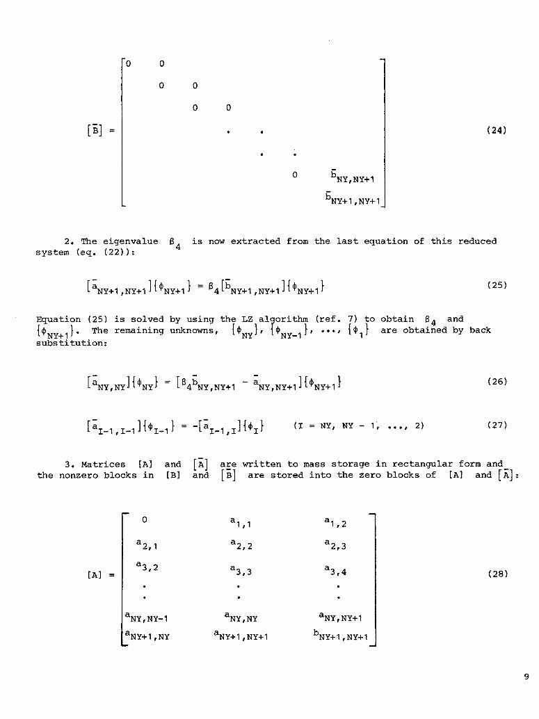
[_]_ . . (24)

m

0 bNY,Ny+ 1m

bNY+I,NY+I

2. The eigenvalue 84 is now extracted from the last equation of this reducedsystem (eq• (22)):

[aNY+I ,NY+I]{CNY+I} = 84 [bNy+I,NY+I]{CNY+1} (25)

Equation (25) is solved by using the LZ algorithm (ref. 7) to obtain 84 and

{_NY+1 }. The remaining unknowns, {_Ny }, {_NY_l }, •.., {41} are obtained by backsubs titution:

[aNY,Ny]{_Ny } = [84bNY,Ny+ 1 - aNY,NY+1]{_NY+l } (26)

[a__i,__i]{__I}=m[a__1,_]{._}(_:NY,_Y-I,...,2_ (27)

3. Matrices [A] and [A] are written to mass storage in rectangular form andthe nonzero blocks in [B] and [B] are stored into the zero blocks of [A] and [A]:

D

0 al,I al,2

a2,1 a2,2 a2,3

a3'2 a3,4 (28)[A] = a3'3

• • •

aNY,NY-1 aNY,NY aNY,NY+I

aNY+I,NY aNY+I,NY+I bNY+I,NY+Ip

9

bNy, NY+I al ,I al ,2

a2,1 a2,2 a2,3

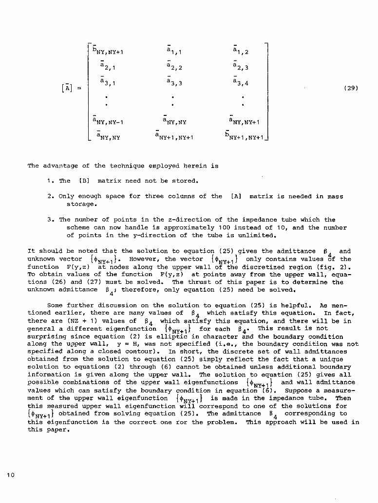
[i] = a3'I a3'3 a3'4 (29)

• • •

aNy, NY- 1 aNy, N g aNy, NY+ I

aNy, NY aNy+ 1, NY+ 1 bNy+ 1, NY+ 1 _

The advantage of the technique employed herein is

1. The [B] matrix need not be stored.

2. Only enough space for three columns of the [A] matrix is needed in massstorage•

3. The number of points in the z-direction of the impedance tube which thescheme can now handle is approximately 100 instead of 10, and the numberof points in the y-direction of the tube is unlimited.

It should be noted that the solution to equation (25) gives the admittance 8 and

unknown vector {_NY+I}" However, the vector {_NY+I} only contains values _f thefunction F(y,z) at nodes along the upper wall of the discretized region (fig. 2).To obtain values of the function F(y,z) at points away from the upper wall, equa-tions (26) and (27) must be solved. The thrust of this paper is to determine the

unknown admittance 84; therefore, only equation (25) need be solved•

Some further discussion on the solution to equation (25) is helpful. As men-

tioned earlier, there are many values of 84 which satisfy this equation. In fact,there are (NZ + I) values of 84 which satisfy this equation, and there will be in

different eigenfunction {#NY+I} for each 84• This result is notgeneral a

surprising since equation (2) is elliptic in character and the boundary conditionalong the upper wall, y = H, was not specified (i.e., the boundary condition was notspecified along a closed contour). In short, the discrete set of wall admittancesobtained from the solution to equation (25) simply reflect the fact that a uniquesolution to equations (2) through (6) cannot be obtained unless additional boundaryinformation is given along the upper wall. The solution to equation (25) gives all

possible combinations of the upper wall eigenfunctions {#NY+I} and wall admittancevalues which can satisfy the boundary condition in equation (6). Suppose a measure-

ment of the upper wall eigenfunction {_NY+I} is made in the impedance tube. Thenthis measured upper wall eigenfunction will correspond to one of the solutions for

{#NY+I} obtained from solving equation (25). The admittance 84 corresponding tothis eigenfunction is the correct one for the problem• This approach will be used inthis paper.

10

RESULTS AND DISCUSSION

In order to verify the numerical technique, results from the method are comparedboth with exact solutions that can be obtained for a uniform mean-flow profile andwith results of reference 4 for cases involving shear in the y-direction only. Next,results are presented for some cases in which the flow possesses shear in both the y-and z-direction of the tube. Results are restricted to a square duct for whichH = L = I foot, K = I (radians per foot), with 50 elements in the y- andz-directions of the tube (NY = NZ = 50). Further, continuity of particle velocity isemployed as the boundary condition and the bottom and side walls of the tube are con-

sidered rigid (81 = 82 = 83 = 0.0 + 0.0i). The choice of this particular combinationof parameters was felt to be sufficient to obtain confidence in the numericaltechnique.

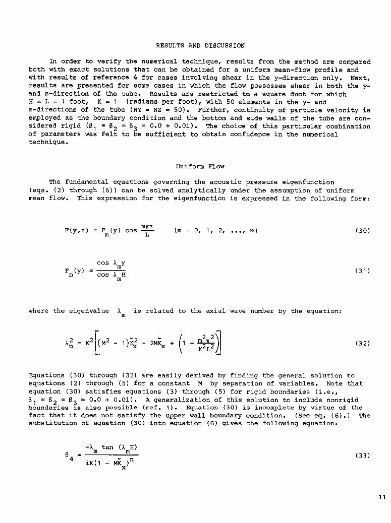
Uniform Flow

The fundamental equations governing the acoustic pressure eigenfunction(eqs. (2) through (6)) can be solved analytically under the assumption of uniformmean flow. This expression for the eigenfunction is expressed in the following form:

m_zF(y,z) = F (y) cos- (m = 0, 1, 2, ..., _) (30)m L

cos ImyF (y) = (31)m cos I Hm

where the eigenvalue 1 is related to the axial wave number by the equation:m

Equations (30) through (32) are easily derived by finding the general solution toequations (2) through (5) for a constant M by separation of variables. Note thatequation (30) satisfies equations (3) through (5) for rigid boundaries (i.e.,

81 = 82 = 83 = 0.0 + 0.0i). A generalization of this solution to include nonrigidboundaries is also possible (ref. I). Equation (30) is incomplete by virtue of thefact that it does not satisfy the upper wall boundary condition. (See eq. (6).) Thesubstitution of equation (30) into equation (6) gives the following equation:

-I tan (I H)

84 = m m (33)iK(1 - MK )nx

11

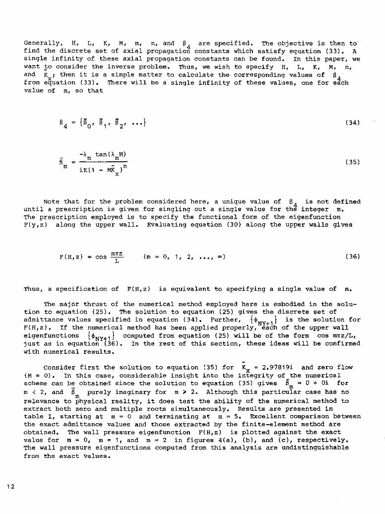
Generally, H, L, K, M, m, n, and 84 are specified. The objective is then tofind the discrete set of axial propagation constants which satisfy equation (33). Asingle infinity of these axial propagation constants can be found. In this paper, wewant to consider the inverse problem. Thus, we wish to specify H, L, K, M, n,

and Kx; then it is a simple matter to calculate the corresponding values of 84from equation (33). There will be a single infinity of these values, one for eachvalue of m, so that

84-- } (34)

-Im tan(ImH)= ¢35)m im(1 - MK )n

x

Note that for the problem considered here, a unique value of 8A is not definedsntil a prescription is given for singling out a single value for th_ integer m.The prescription employed is to specify the functional form of the eigenfunctionF(y,z) along the upper wall. Evaluating equation (30) along the upper walls gives

F(H,z) = cos m_____z (m = 0, I, 2, ..., _) (36)L

Thus, a specification of F(H,z) is equivalent to specifying a single value of m.

The major thrust of the numerical method employed here is embodied in the solu-tion to equation (25). The solution to equation (25) gives the discrete set of

admittance values specified in equation (34). Further, {@NY+1} is the solution forF(H,z). If the numerical method has been applied properly, each of the upper wall

eigenfunctions {@NY+I} computed from equation (25) will be of the form cos m_z/L,just as in equation (36). In the rest of this section, these ideas will be confirmedwith numerical results.

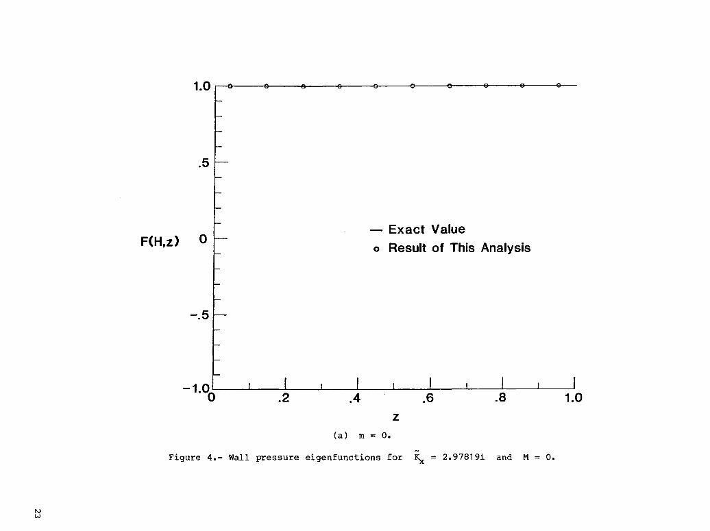
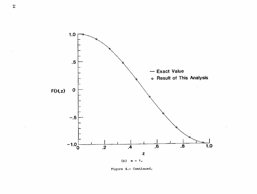
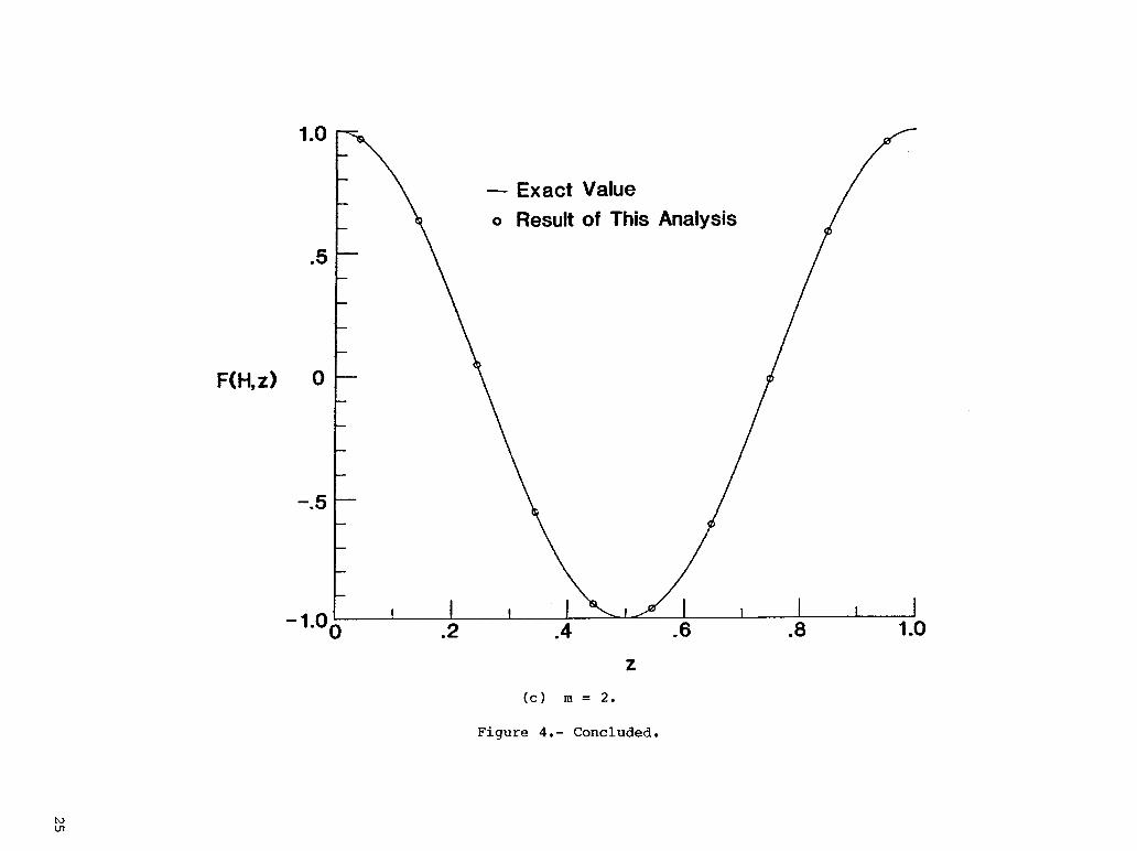
Consider first the solution to equation (35) for Kx = 2.97819i and zero flow(M = 0). In this case, considerable insight into the integrity of the numericalscheme can be obtained since the solution to equation (35) gives 8 = 0 + 0i formm < 2, and 8 purely imaginary for m ) 2. Although this particular case has nomrelevance to physical reality, it does test the ability of the numerical method toextract both zero and multiple roots simultaneously. Results are presented intable I, starting at m = 0 and terminating at m = 5. Excellent comparison betweenthe exact admittance values and those extracted by the finite-element method areobtained. The wall pressure eigenfunction F(H,z) is plotted against the exactvalue for m = 0, m = 1, and m = 2 in figures 4(a), (b), and (c), respectively.The wall pressure eigenfunctions computed from this analysis are undistinguishablefrom the exact values.

12

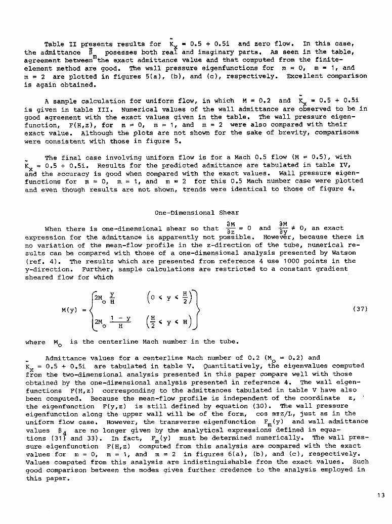
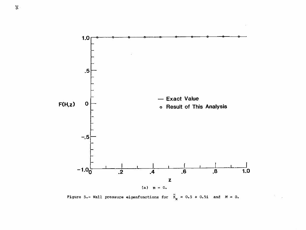
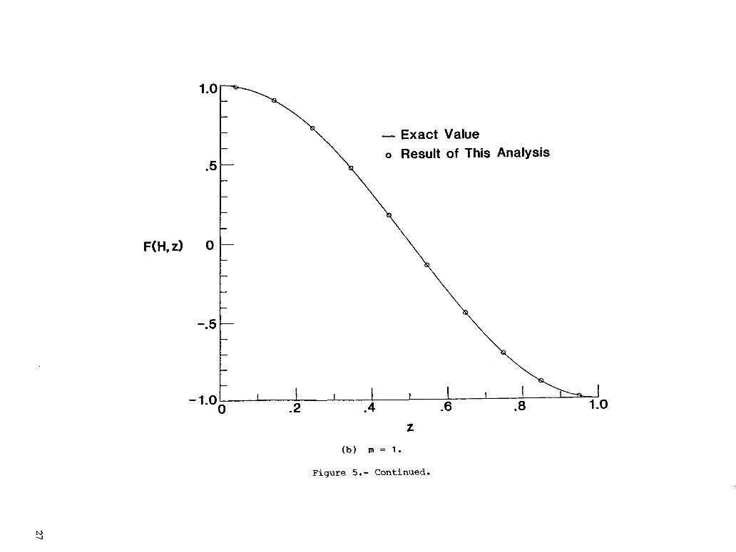
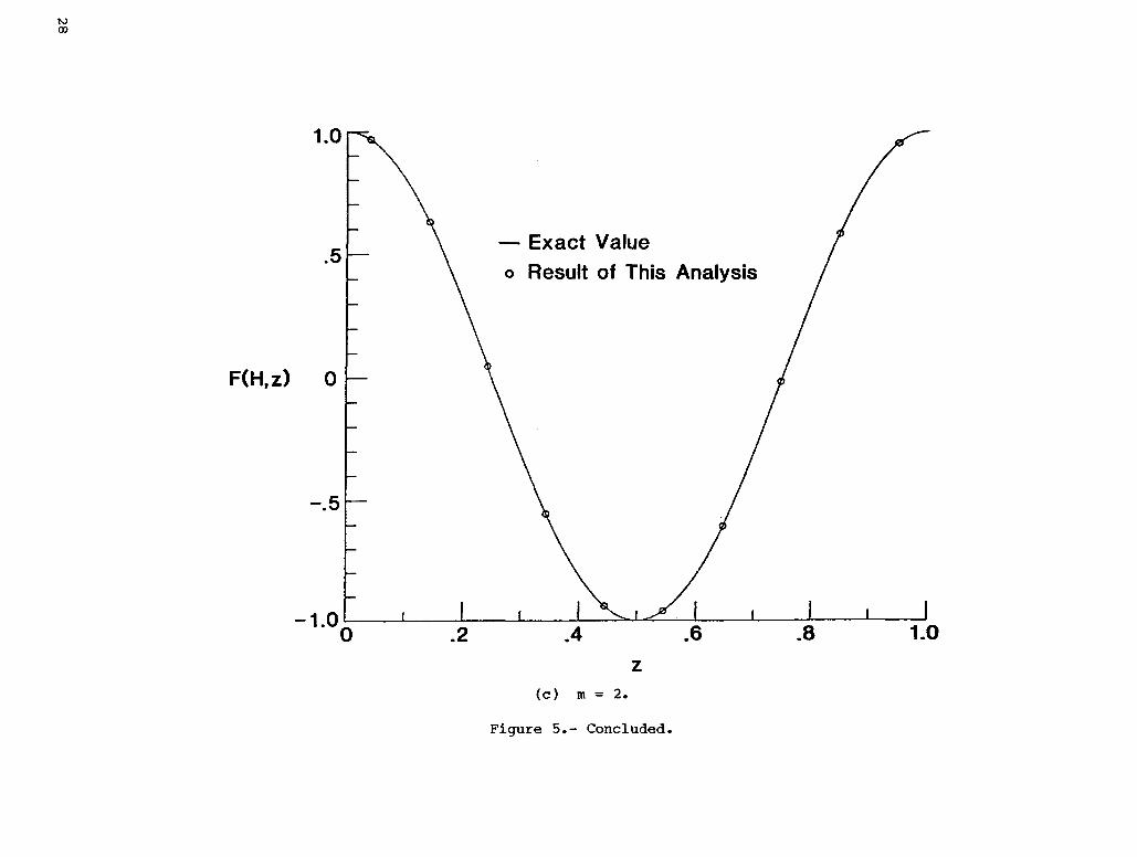
Table II presents results for Kx = 0.5 + 0.5i and zero flow. In this case,the admittance _ posesses both real and imaginary parts. As seen in the table,magreement between the exact admlttance value and that computed from the finite-element method are good. The wall pressure eigenfunctions for m = 0, m = I, andm = 2 are plotted in figures 5(a), (b), and (c), respectively. Excellent comparisonis again obtained.

A sample calculation for uniform flow, in which M = 0.2 and Kx = 0.5 + 0.5iis given in table III. Numerical values of the wall admittance are observed to be ingood agreement with the exact values given in the table. The wall pressure eigen-function, F(H,z), for m = 0, m = I, and m = 2 were also compared with theirexact value. Although the plots are not shown for the sake of brevity, comparisonswere consistent with those in figure 5.

The final case involving uniform flow is for a Mach 0.5 flow (M = 0.5), with

Kx = 0.5 + 0.5i. Results for the predicted admittance are tabulated in table IV,and the accuracy is good when compared with the exact values. Wall pressure eigen-functions for m = 0, m = I, and m = 2 for this 0.5 Mach number case were plottedand even though results are not shown, trends were identical to those of figure 4.

0ne-Dimensional Shear

8M _MWhen there is one-dimensional shear so that _ = 0 and -_7_# 0, an exact

expression for the admittance is apparently not possible. However, because there isno variation of the mean-flow profile in the z-direction of the tube, numerical re-sults can be compared with those of a one-dimensional analysis presented by Watson(ref. 4). The results which are presented from reference 4 use 1000 points in they-direction. Further, sample calculations are restricted to a constant gradientsheared flow for which

where Mo is the centerline Mach number in the tube.

Admittance values for a centerline Mach number of 0.2 (Mo = 0.2) and

Kx = 0.5 + 0.5i are tabulated in table V. Quantitatively, the eigenvalues computedfrom the two-dimensional analysis presented in this paper compare well with thoseobtained by the one-dimensional analysis presented in reference 4. The wall eigen-functions F(H,z) corresponding to the admittances tabulated in table V have alsobeen computed. Because the mean-flow profile is independent of the coordinate z,the eigenfunction F(y,z) is still defined by equation (30). The wall pressureeigenfunction along the upper wall will be of the form, cos m_z/L, just as in the

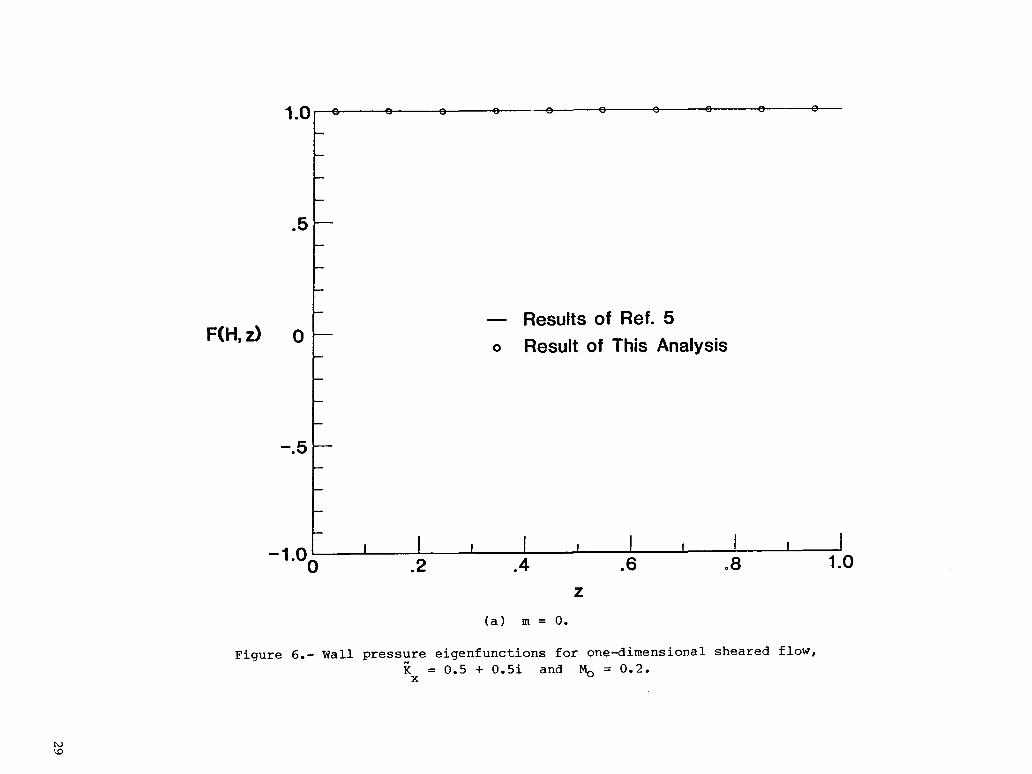
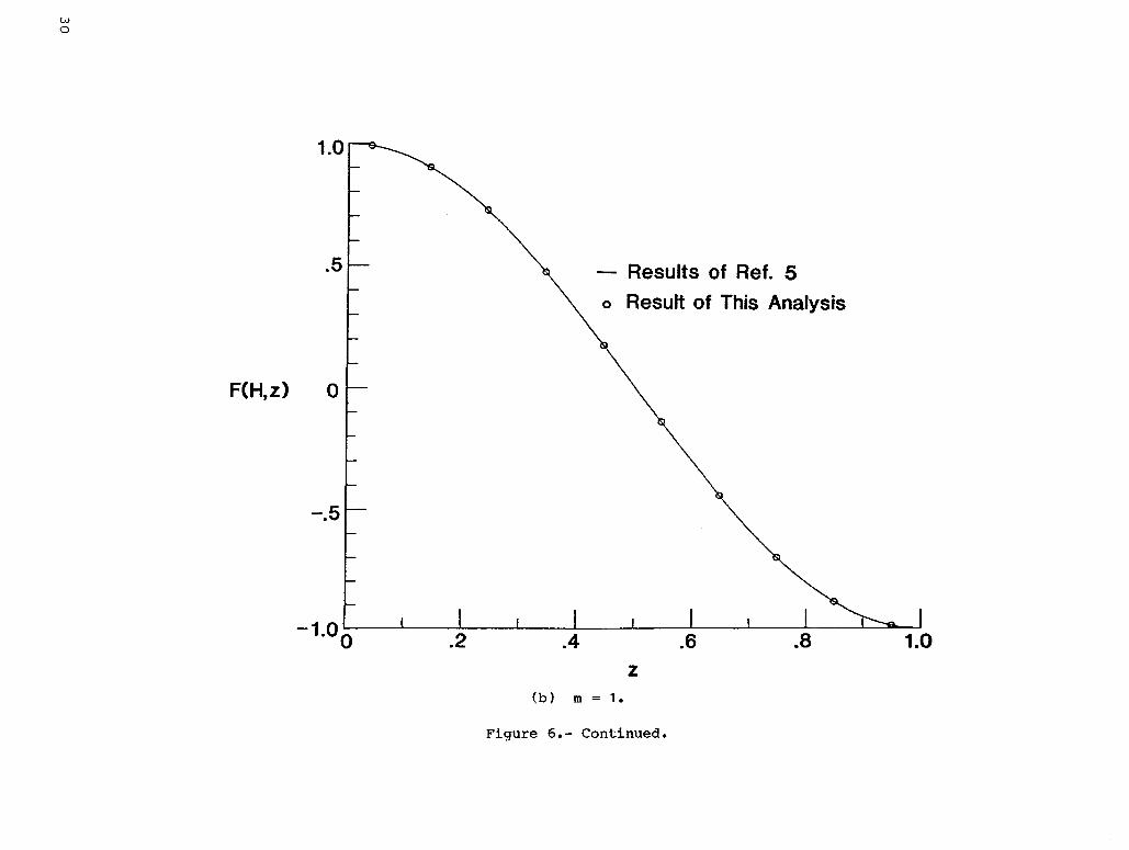
uniform flow case. However, the transverse eigenfunction Fm(Y) and wall admittancevalues 84 are no longer given by the analytical expressions defined in equa-tions (31) and 33). In fact, Fm(Y) must be determined numerically. The wall pres-sure eigenfunction F(H,z) computed from this analysis are compared with the exactvalues for m = 0, m = 1, and m = 2 in figures 6(a), (b), and (c), respectively.Values computed from this analysis are indistinguishable from the exact values. Suchgood comparison between the modes gives further credence to the analysis employed inthis paper.

13

The final sample calculation is for M = 0.5 and Kx = 0.5 + 0.5i. Admittancecalculations are given in table VI. Note that for this reasonably high centerlineMach number, the admittance values computed from this analysis compare well withthose computed from reference 4. The wall pressure eigenfunction, F(H,z), form = 0, m = I, and m = 2 were consistent with those in figure 6.

Two-Dimensional Shear

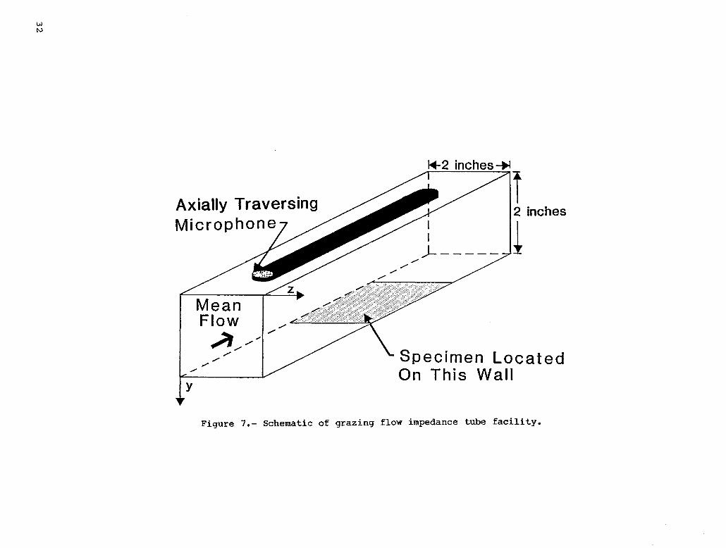
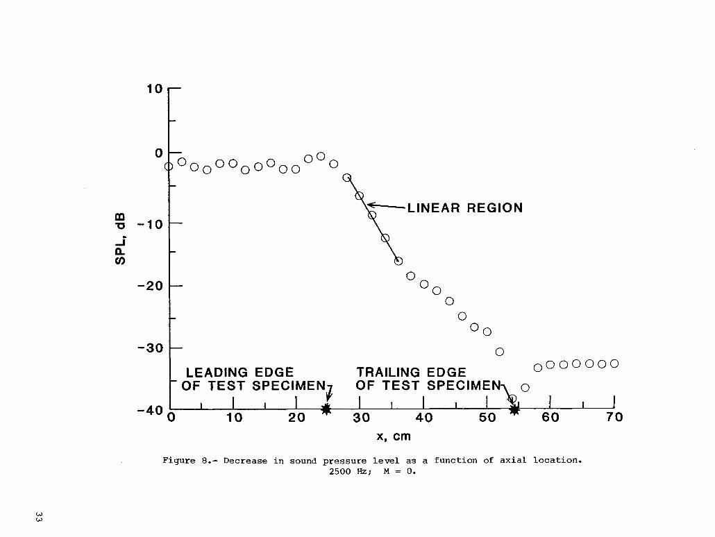
Results are now presented for a flow containing gradients in both cross-sectional directions of an impedance tube. In this final example, a demonstration ofhow data taken from a two-dimensional sheared flow experiment are used in conjunctionwith the analysis presented here to determine the admittance of a test specimen isgiven. The experimental data were obtained in the flow impedance test laboratory atthe Langley Research Center.

A sketch of the grazing flow impedance tube is shown in figure 7. The tube is2 inches square, so that H = L = 2 inches, and the data were obtained at 2500 hertz.Note that the origin of the coordinate system is chosen in the upper left-hand cornerof the tube, so that the test specimen is located on the upper wall when referencedto this origin. Data obtained from the axially transversing microphone establish theattenuation and phase rate characteristics along the length of the test specimen.Attenuation and phase rate data are translated directly into an axial propagationconstant (ref. 2).

A plot of sound pressure level (SPL) in decibels as a function of axial distanceat 2500 Hz and M = 0 is shown in figure 8. The leading and trailing edge of thetest specimen is denoted by an asterisk on the X-axis. It is of interest to notethat the slope of the curve in figure 8 at axial position x gives the attenuationrate at the position. Further, the curve is linear in regions which are dominated bya single propagating mode. The standing wave patterns in the vicinity of the leadingand trailing edge of the specimen indicate the presence of reflections and higherorder mode contamination. The analysis presented in this paper is not applicable inthese regions because of the presence of multiple modes in the acoustic field. How-ever, the curve is clearly linear for values of x between 27 and 35 centimeters.It is this linear portion of the curve that was used to obtain the attenuation rate.Although the curve is not shown, phase rate data show trends similar to that in fig-ure 8 with the linear portion of the curve covering a much wider range of valuesof x.

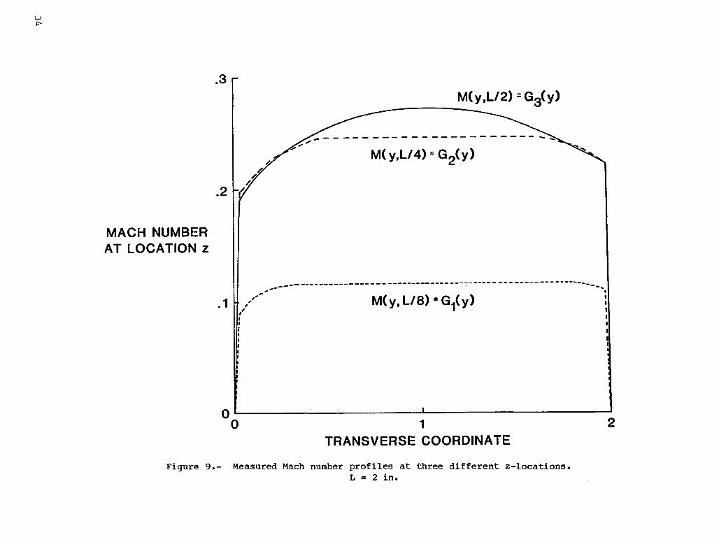
The mean-flow profile in the tube was obtained by aerodynamic measurements, atthe 350 points in the cross section. The node points for the finite elements werechosen at points in the domain where mean flow measurements were taken (i.e., NZ = 9and NY = 34). Figure 9 gives a graphical representation of the flow profile mea-sured in the tube as a function of the coordinate y, at z = I, I/2, and I/4 inch.Note that the functional form of the mean-flow profile changes at each of the threez stations so that this profile is not independent of the coordinate z as in theprevious section. Further, the centerline Mach number of this profile was determined

to be approximately 0.3 (MO = 0.3).

A sample calculation is shown in table VII for no flow, uniform flow, a flowwith one-dimensional shear, and the measured flow. The admittance given in the tablecorresponds to the admittance of the mode which is closest to a plane wave. The flowwith one-dimensional shear was constructed by using the profile at z = L/2 in fig-

ure 9 (i.eo, M(y,z) = G3(Y)), whereas the uniform flow value was chosen as the

)average value of G3(Y) .e., M = G3(Y) dy . Results show that uniform flow

calculations agree better with results for one-dimensional shear than the no-flowcalculation. Further, the uniform flow profile with the particle displacementcontinuity (n = 2) as the boundary condition, agrees better with the one-dimensionalshear results than the particle velocity boundary condition (n = I). Note that theuniform flow and one-dimensional sheared flow admittance value differ only moderatelyfrom the zero flow value. In contrast the imaginary part of the admittance calcu-lated by using the measured profile, differs significantly from that calculated fromthe profile with only one-dimensional shear. Such results suggest that for flowsover acoustically lined panels, the flow has a significant effect on the acousticproperties of the liner. The reader is reminded however, that this result would beinvalidated if the measured value of the wall pressure eigenfunction F(H,z) did notcoincide with that calculated from the two-dimensional sheared flow analysis.Unfortunately, measurements of the upper wall eigenfunction were not available andcould not be compared with values computed from this analysis.

CONCLUDING REMARKS

A method has been developed for calculating the acoustic admittance of a testspecimen located within the wall of a grazing flow impedance tube with flow gradientsin both cross-sectional directions. The method, developed and tested for rectangulartubes, may be extended to other geometries as well. In this approach, the unknownadmittance value is assumed constant and is obtained by solving an eigenvalue prob-lem. This eigenvalue problem results from the application of the finite-elementmethod to the partial differential equation and boundary conditions governing theacoustic field. A major effort has been devoted toward the solution to this eigen-value problem, which requires a special scheme to obtain the eigenvalues.

Admittance values determined from the method were compared with exact solutionsobtained for a constant mean-flow profile and with results of NASA Technical Paper2310 for cases involving shear in a single cross-sectional direction. Excellentcomparisons were obtained giving credibility to the scheme. Results have been givenfor the first time in which the flow is represented realistically with gradients inboth cross-sectional directions. Limited results obtained for a test specimeninstalled in the wall of the flow impedance test laboratory at the Langley ResearchCenter suggest that grazing flows can have a significant impact on the acousticadmittance.

NASA Langley Research CenterHampton, VA 23665-5225August 23, 1985

15

REFERENCES

I. Kraft, Robert Eugene: Theory an_ Measurement of Acoustic Wave Propagation inMulti-Segmented Rectangular Flow Ducts. Ph.D. Diss., Univ. of Cincinnati, 1976.

2. Armstrong, D. L.; Beckemeyer, R. J.; and Olsen, R. F.: Impedance Measurements ofAcoustic Duct Liners With Grazing Flow. Boeing paper presented at 87th Meetingof the Acoustical Society of America (New York, New York), Apr. 1974.

3. Mungur, P.; and Gladwell, G. M. L.: Acoustic Wave Propagation in a Sheared FluidContained in a Duct. J. Sound & Vib.; vol. 9, no. I, Jan. 1969, pp. 28-48.

4. Watson, Willie R: A New Method for Determining Acoustic-Liner Admittance in aRectangular Duct With Grazing Flow From Experimental Data. NASA TP-2310, 1984.

5. Unruh, J. F.; and Eversman, W.: The Transmission of Sound in an AcousticallyTreated Rectangular Duct With Boundary Layer. J. Sound & Vib., vol. 25, no. 3,Dec. 1972, pp. 371-382.

6. Desai, Chandrakant S.; and Abel, John F.: Introduction to the Finite ElementMethod - A Numerical Method for Engineering Analysis. Van Nostrand ReinholdCo., c.1972.

7. Kaufman, Linda: Algorithm 496 - The LZ Algorithm to Solve the Generalized Eigen-value Problem for Complex Matrices [F2]. ACM Trans. Math. Software, vol. I,no. 3, Sept. 1975, pp. 271-281.

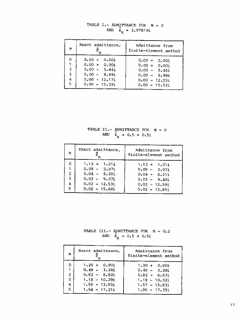
TABLE I.- ADMITTANCE FOR M = 0

AND K = 2. 97819ix

Exact admittance, Admittance from

m _m finite-element method

0 0.00 + 0.00i 0.00 + 0.00i

I 0.00 + 0.00i 0.00 + 0.00i

2 0.00 - 5.44i 0.00 - 5.45i

3 0.00 - 8.89i 0.00 - 8.98i

4 0.00 - 12.17i 0.00 - 12.23i

5 0.00 - 15.39i 0.00 - 15.52i

TABLE II.- ADMITTANCE FOR M = 0

AND K = 0.5 + 0.5ix

Exact admittance, Admittance from

m _ finite-element methodm

0 1.13 + 1.21i 1.13 + 1.21iI 0.09 - 2.97i 0.09 - 2.97i2 0.04 - 6.20i 0.04 - 6.21i3 0.03 - 9.37i 0.03 - 9.40i4 0.02 - 12.53i 0.02 - 12.59i5 0.02 - 15.68i 0.02 - 15.81i

TABLE III.- ADMITTANCE FOR M = 0.2

AND Kx = 0.5 + 0.5i

Exact admittance, Admittance fromm _ finite-element methodm

0 1.20 + 0.90i 1.20 + 0.90i1 0.49 - 3.28i 0.49 - 3.28i2 0.82 - 6.82i 0.82 - 6.83i3 1.18- I0.29i 1.19- I0.32i4 1.56 - 13.95i 1.57 - 13.83i5 1.94 - 17.21i 1.95 - 17.35i

17

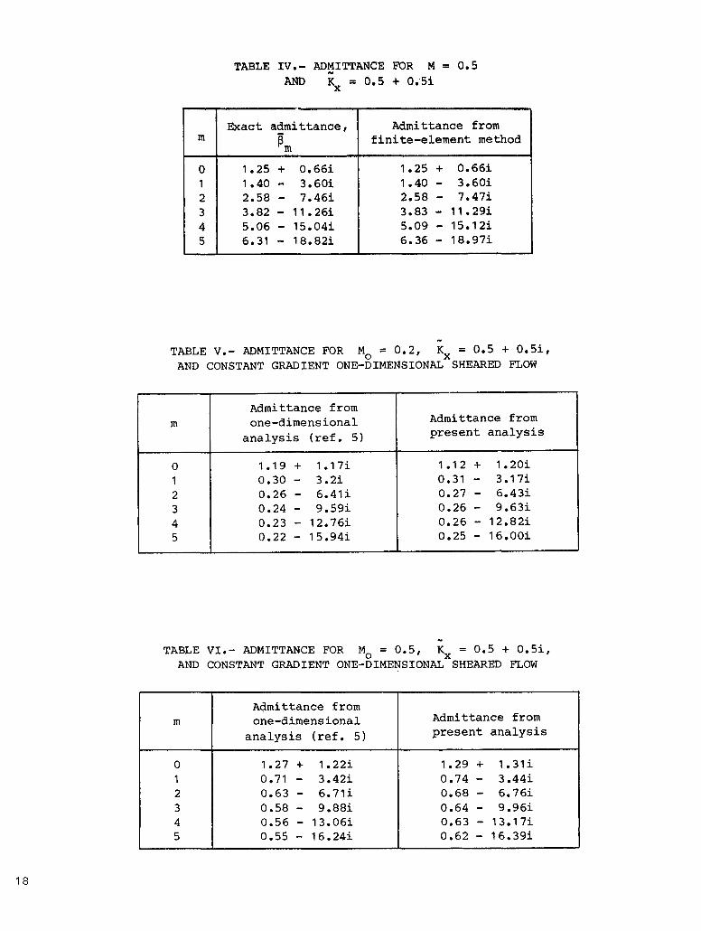
TABLE IV,- ADMITTANCE FOR M = 0.5

AND Kx = 0.5 + 0.5i

Exact admittance, Admittance from

m _m finite-element method

0 1.25 + 0.66i 1.25 + 0.66iI 1.40 - 3.60i 1.40 - 3.60i2 2.58 - 7.46i 2.58 - 7.47i3 3.82 - 11.26i 3.83 - 11.29i4 5.06 - 15.04i 5.09 - 15.12i5 6.31 - 18.82i 6.36 - 18.97i

TABLE V.- ADMITTANCE FOR Mo = 0.2, Kx = 0.5 + 0.5i,AND CONSTANT GRADIENT ONE-DIMENSIONAL SHEARED FLOW

Admittance fromm one-dimensional Admittance from

analysis (ref. 5) present analysis

0 1.19 + 1.17i 1.12 + 1.20i1 0.30 - 3.2i 0.31 - 3.17i2 0.26 - 6.41i 0.27 - 6.43i3 0.24 - 9.59i 0.26 - 9.63i4 0.23 - 12.76i 0.26 - 12.82i5 0.22 - 15.94i 0.25 - 16.00i

TABLE VI.- ADMITTANCE FOR Mo = 0.5, Kx = 0.5 + 0.5i,AND CONSTANT GRADIENT ONE-DIMENSIONAL SHEARED FLOW

Admittance fromm one-dimensional Admittance from

analysis (ref. 5) present analysis

0 1.27 + 1.22i 1.29 + 1.31iI 0.71 - 3.42i 0.74 - 3.44i2 0.63 - 6.71i 0.68 - 6.76i3 0.58 - 9.88i 0.64 - 9.96i4 0.56 - 13.06i 0.63 - 13.17i5 0.55 - 16.24i 0.62 - 16.39i

18

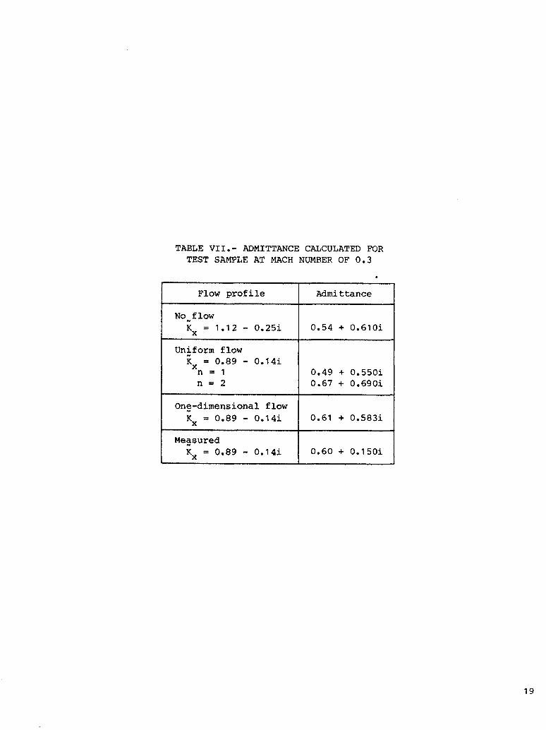
TABLE VII.- ADMITTANCE CALCULATED FORTEST SAMPLE AT MACH NUMBER OF 0.3

Flow profile Admittance

No flow

Kx = 1.12 - 0.25i 0.54 + 0.610i

Uniform flowK = 0.89 - 0.14ixn = I 0.49 + 0.550in = 2 0.67 + 0.690i

On£-dimensional flow

Kx = 0.89 - 0.14i 0.61 + 0.583i

Measured

K_ = 0,89 - 0.14i 0.60 + 0.150ii

19

o

Figure I.- Grazing flow impedance tube and coordinate system.

Y

I-t

(NY,1) (NY,2) (NY,3) [NY,NZ_

YNY

(2,1) (2,2) (2,3) (2,NZ)

Y2 _z+311',iz+3J

(1,1) (1,2) (1,3) (1,NZ)

zI z2 z3 zNZ L Z

Figure 2.- Finite-element discretization.

t_

Global Coordinate System Local Coordinate System

q=Y-YjY q _=z-z I

a= Zl+l-Z Ib =YJ+I-5

YJ.l ._ _ b_

z I Zl+1 z 0 a _-

Figure 3.- Global and local coordinate system for a typical finite element.

.0 0 0 C C 0 0 0 0 0 0

.5 --

-- Exact ValueF(H,z) 0 --_ o Result of This Analysis

_e5

-1.n, , ! , I , I , I , i-o .2 .4 .6 .8 1.0Z

(a) m = 0.

Figure 4.- Wall pressure eigenfunctions for Kx = 2.97819i and M = 0.

5Ot_

h3

1.0

.5

-- Exact Value

F(H,z) 0 t of This Analysis

--.5

-10 110• 0 .2 .4 • • -Z

(b) m = I.

Figure 4.- Continued.

1.0

-- Exact Value

o Resultof This Analysis

.5

FIll, z) 0 --N

_u5

m

, ! t I I , I , I-1"00 .2 .4 .6 .8 1.0

Z

(C) m = 2.

Figure 4.- Concluded.

hJU1

t_o_

I O ^ "_ ^ _ 0 " 0 _, _,u

.5

- N Exact ValueF(H,z) 0 -- o Result of This Analysis

m

_1.06 v I v I I ! t ! ! l.2 .4 .6 .8 1.0Z

(a) m = O.

Figure 5.- Wall pressure eigenfunctions for _ = 0.5 + 0.5i and M = 0.

1"Ok -__ m Exact Value_[ _ o Result of This Analysis

FIN, z)

--.5

-1 o Io• 0 .2 .4 . . -Z

(b) m = 1.

Figure 5.- Continued.

h_-J

boCO

1.0

.5 -- Exact Valueo Result of This Anal "

F(H,z) 0

_e5 --

_1.00 _ I , t I I I.2 .4 .6 .8 1.0Z

(c) m = 2.

Figure 5.- Concluded.

.0 _ "_ 0 0 0 0 O. 0 0 0

.5

- -- Results of Ref. 5F(H,z) 0 -- o Result of This Analysis

m

m=5

m

m

_1.00 ! ! , I , I q I w i.2 .4 .6 .8 1.0Z

(a) m = 0.

Figure 6.- Wall pressure eigenfunctions for one-dimensional sheared flow,K = 0.5 + 0.5i and Mo = 0.2.x

bo%O

L_0

1.0

.5 -- Results of Ref. 5

F(H,z) 0 is Analysis

q I w I i I I-1"00 .2 .4 .6 .8 1.0

Z

(b) m = 1.

Figure 6.- Continued.

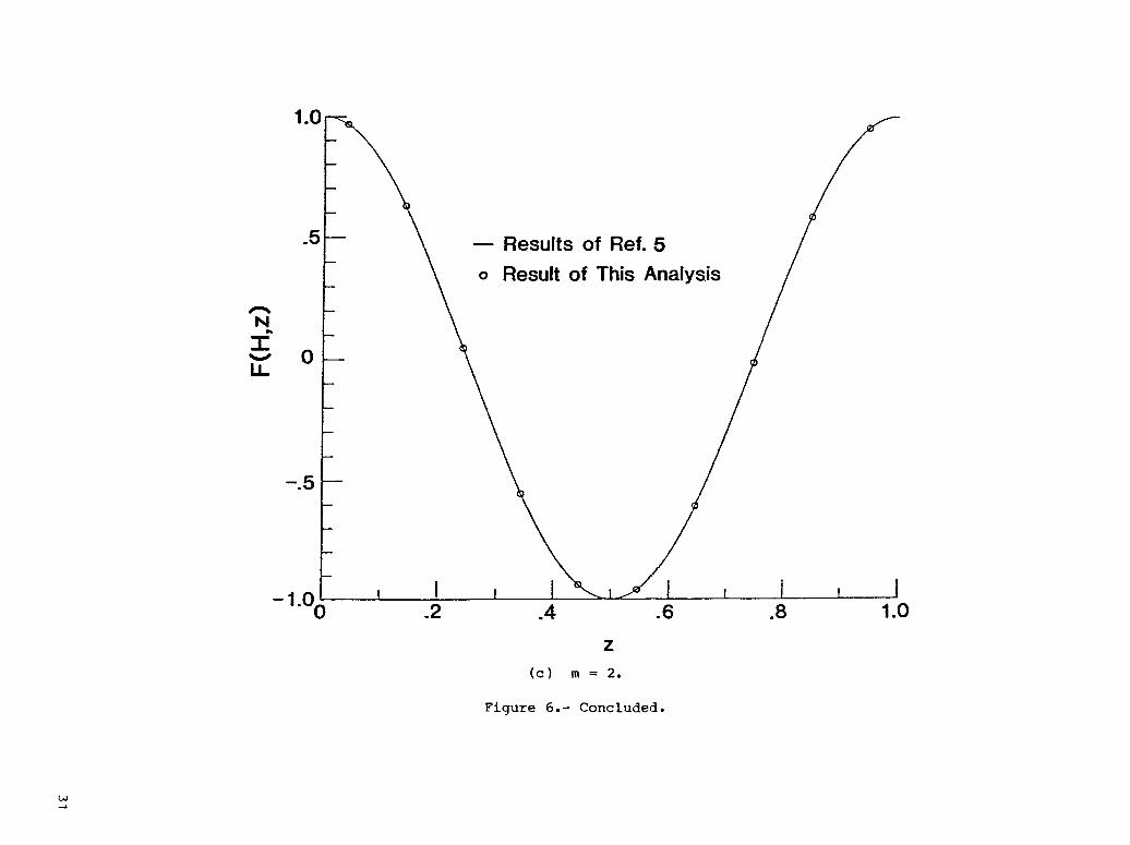
1.0 •

.5- _ -- Results of Ref. 5

N-r"

0LL

m

_1.Oo , I , I "%..,.J I , I , I.2 .4 .6 .8 1.0

Z

(C) m = 2.

Figure 6.- Concluded.

L_

L,Ot_

Figure 7.- Schematic of grazing flow impedance tube facility.

10--

O m oOOooOOooOoo o

LINEAR REGIONrn"o -10 --J

O-20 -- 0 0

0- 0

0 o

-30 -- o

LEADING EDGE TRAILING EDGE oO O O O OO

- ,OF TE T SPECIMEN.-/ F TEST SPECl, !

' ' _0 "_ '410'5 I 610 70-40 0 10 30 0

X, cm

Figure 8.- Decrease in sound pressure level as a function of axial location.2500 Hz; M = 0.

L_%0

%o

3-

M(y,L/2) =G3(Y)

_/"- Mly,L/4) =G2(Y )

MACH NUMBERAT LOCATION z

.1 ,'° M(y,L/8) =Gl(Y)f

I

00 1 2TRANSVERSE COORDINATE

Figure 9.- Measured Mach number profiles at three different z-locations.L = 2 in.

L.O

1. Re_rt No. 2. GovernmentAccmion No. 3, Recipieflt't CatalogNo.

NASA TP- 25184. Title and Subtitle 5. Report Date

A Method for Determining Acoustic-Liner Admittance October 1985

in Ducts With Sheared Flow in Two Cross-Sectional 6. PerformingOrganizationCodeDirections 505-31-33-13

7, Author(s) 8. Performing Organization Report No.

Willie R. Watson L-15997

10. Work LJnitNo.

9. PerformingOrganizationName andAddress

NASA Langley Research Center 11 ContractorGrantNo.Hampton, VA 23665-5225

13. Type of Report and PeriodCovered

12 S_onsoringAgencyNameandAddress Technical Paper

National Aeronautics and Space Administration 14.SponsoringAgencyCodeWashington, DC 20546-0001

15. Supplementary Notes

,, ,,,,

16. Abstract

A method is developed for determining the acoustic admittance of a test liner in-stalled in the wall of a grazing flow impedance tube. The mean flow is permittedflow gradients in both cross-sectional directions of the tube. The unknown admit-tance value is obtained by solving an eigenvalue problem. This eigenvalue problemresults from the application of the finite-element method to the partial differentialequation and boundary conditions governing the acoustic field. The credibility ofthe method is established by comparing results with exact solutions obtained for aconstant mean-flow profile and with previous results for cases involving shear inonly one cross-sectional direction. Excellent comparisons were obtained in bothcases. The analysis has been used in conjunction with a limited amount of experimen-tal data and shows that the flow must be accurately modeled in order to determine theacoustic-liner properties.

i

17. Key Words(Suggest_ by Author(s)) 18. Distributi_ S_tement

Duct acoustics Unclassified - UnlimitedAcoustic impedanceSuppressionSound-absorbing materials

Subject Category 71

19, Security _auif.(ofthisre_rt) 20. SecurityClauif.(ofthi$ _) 21. No. of Pages 22. _ice

36 Unclassified Unclassified 37 A03

,-3o5 ForsalebytheNationalTechnicalInf_mationService,Springfield,Virginia22161

NationalAeronauticsandSpaceAdministrationCodeNIT-3 3 1176 01358 4876 BULKRATE- _ ° POSTAGE & FEES PAID

NASA Washington,DCWashington,D.C. PermitNo. G-2720546-0001

Official BusinessPenalty to, Private Use, S300

If Undeliverable 1$8(SectionPOSTMASTER

Postal Manual) Do Not Return