Directional virtual backbone based data aggregation scheme

RESEARCH ARTICLE

Directional virtual backbone based data

aggregation scheme for Wireless Visual

Sensor Networks

Jing Zhang1*, Shi-jian Liu1, Pei-Wei Tsai2, Fu-min Zou1, Xiao-rong Ji1

1 School of Information Science and Engineering, Fujian University of Technology, and Fujian Provincial Key

Laboratory of Big Data Mining and Applications, Fuzhou, China, 2 Department of Computer Science and

Software Engineering, Swinburne University of Technology, Hawthorn, Australia

* [email protected]

Abstract

Data gathering is a fundamental task in Wireless Visual Sensor Networks (WVSNs). Fea-

tures of directional antennas and the visual data make WVSNs more complex than the con-

ventional Wireless Sensor Network (WSN). The virtual backbone is a technique, which is

capable of constructing clusters. The version associating with the aggregation operation is

also referred to as the virtual backbone tree. In most of the existing literature, the main focus

is on the efficiency brought by the construction of clusters that the existing methods neglect

local-balance problems in general. To fill up this gap, Directional Virtual Backbone based

Data Aggregation Scheme (DVBDAS) for the WVSNs is proposed in this paper. In addition,

a measurement called the energy consumption density is proposed for evaluating the ade-

quacy of results in the cluster-based construction problems. Moreover, the directional virtual

backbone construction scheme is proposed by considering the local-balanced factor. Fur-

thermore, the associated network coding mechanism is utilized to construct DVBDAS.

Finally, both the theoretical analysis of the proposed DVBDAS and the simulations are given

for evaluating the performance. The experimental results prove that the proposed DVBDAS

achieves higher performance in terms of both the energy preservation and the network life-

time extension than the existing methods.

Introduction

Wireless Sensor Networks (WSNs) consist of geographically distributed sensors that commu-

nicate with each other over wireless channels. A particular branch, which is equipped with the

visual sensors for capturing target events through the video acquisition, called the Wireless

Visual Sensor Network (WVSN) delivers the digital visual information via the wireless chan-

nels to the control unit further data analysis and decision making [1]. The WVSNs have a wide

range of applications, such as visual security surveillance and visual wildlife monitoring [2].

The energy consumption pattern of the WVSN is very different from the conventional WSN.

The reason is that the transmitted information in the conventional WSN are relatively small

PLOS ONE | https://doi.org/10.1371/journal.pone.0196705 May 15, 2018 1 / 27

a1111111111

a1111111111

a1111111111

a1111111111

a1111111111

OPENACCESS

Citation: Zhang J, Liu S-j, Tsai P-W, Zou F-m, Ji X-

r (2018) Directional virtual backbone based data

aggregation scheme for Wireless Visual Sensor

Networks. PLoS ONE 13(5): e0196705. https://doi.

org/10.1371/journal.pone.0196705

Editor: Lixiang Li, Beijing University of Posts and

Telecommunications, CHINA

Received: November 9, 2017

Accepted: April 18, 2018

Published: May 15, 2018

Copyright: © 2018 Zhang et al. This is an open

access article distributed under the terms of the

Creative Commons Attribution License, which

permits unrestricted use, distribution, and

reproduction in any medium, provided the original

author and source are credited.

Data Availability Statement: All relevant data are

within the paper and its Supporting Information

files.

Funding: Dr. Jing Zhang received support from the

Natural Science Foundation of Fujian Province of

China (2017J05098) and (JK2017029), the

Education Department of Fujian Province science

and technology project (JAT160328), and the

Education Department of Fujian Province science

and technology project (JZ160461). The URLs of

the project is as follows: http://xmgl.fjkjt.gov.cn/p_

itemsearch.pr.pr_iteminfo_public_index.do?I_

https://doi.org/10.1371/journal.pone.0196705

http://crossmark.crossref.org/dialog/?doi=10.1371/journal.pone.0196705&domain=pdf&date_stamp=2018-05-15








http://creativecommons.org/licenses/by/4.0/

http://xmgl.fjkjt.gov.cn/p_itemsearch.pr.pr_iteminfo_public_index.do?I_ITEMID=73203&I_ITEMTYPEID=4


because it is generally digit data collected by the sensors with a single value or a few set of val-

ues. However, in the WVSN, the transmitted data is the video sequence, which is still much

larger than the digit data even after the compression. Thus, the energy consumption of the

WVSN is much larger than the conventional WSN [3]. In addition, the origin of inventing the

WSN system is to create a wireless sensing and data transmission system under extreme envi-

ronments such as the war zone, the large area of wasteland, or the disaster scene. The sensors

are designed as disposable modules composed of a battery, a sensor unit, and a communica-

tion unit. It means that replacing or recharging the battery is impractical and sometimes

impossible. Hence, designing the efficient data transmission protocols and routing algorithms

are critical problems for the WVSNs to reduce the energy consumption in most applications.

In order the reduce the energy consumption caused by the data transmission, most of the

WVSNs utilize the directional antenna to gain the equivalent transmission ability to the omni-

directional antenna but with lower energy consumption. With the directional sensors, a sensor

node can sense partial sectors of a disk, which is centered at itself with the adjustable antenna

[4]. The directional antenna [5] has a number of advantages over the omnidirectional antenna.

By focusing energy only in the intended direction, the directional antenna is capable to

increase the potential for spatial reuse and can provide longer transmission/reception distance

than the omnidirectional antenna with the same amount of power consumption. The partially

switched on sectors of a disk by the directional sensor node limits the toward direction of data

forwarding but also reduces both the energy consumption for transmitting the data and the

interference with other nodes. Different from the omnidirectional sensors, the discrete target

coverage in the directional sensor network environment is determined by both the location

and the orientation of the sensors. Thus, the complexity of routing and system optimization is

significantly increased in the directional sensor networks such as the WVSNs. Since the char-

acteristics of the directional sensor network and the omnidirectional sensor network is differ-

ent, many existing methods used in the omnidirectional sensor network environments are not

adaptable for using in the directional sensor network environments [6–9]. The need of intelli-

gent schemes for capturing, processing, and transmitting visual data with the WVSNs with the

resource-limited environment is undeniable. Answering to the need mentioned above, a

Directional Virtual Backbone based Data Aggregation Scheme (DVBDAS) is proposed in this

paper for solving the energy consumption optimization problem in the WVSNs. Our proposed

scheme is capable to minimize the energy consumption but maximize the network lifetime by

combining the clustering algorithm, the directional virtual backbone construction algorithm,

and the network coding mechanism. The main contributions of this paper are listed as follows:

(1) A scheme called Directional Virtual Backbone based Data Aggregation Scheme

(DVBDAS) for minimizing the power consumption and maximizing the network lifetime in

the Wireless Visual Sensor Networks is proposed. The proposed scheme contains three proce-

dures: the cluster construction, the directional virtual backboard generation, and the network

coding mechanism deployment. In the DVBDAS structure, each cluster collects data from its

own cluster. The cluster head forwards the collected data to the sink node through the route

constructed by the virtual backbone data aggregation tree.

(2) A novel measurement called the energy consumption density (Dec) is defined in this

paper for determining the cluster heads of all clusters by considering the load balance in the

clusters. The defined Dec provides answers to the crucial adapted cluster construction problem.

(3) An associated network coding and the directional control directional virtual backbone

construction algorithm is proposed in this paper for building the energy preservation data

aggregation tree in the WVSNs.

The rest of this paper is organized as follows: the related works of the topology control

based data aggregation is briefly reviewed in section 2. Models and assumptions are defined in

Directional virtual backbone based data aggregation scheme for WVSN


ITEMID=73203&I_ITEMTYPEID=4. The funders

had no role in study design, data collection and

analysis, decision to publish, or preparation of the

manuscript.

Competing interests: The authors have declared

that no competing interests exist.



section 3. The proposed Directional Virtual Backbone based Data Aggregation Scheme is

described in Section 4. The theoretical analysis and the simulation results are discussed in Sec-

tion 5 and Section 6, respectively. Finally, the conclusion is made in Section 7.

Related works

Topology control is a key issue, which must be addressed in WSNs. Several researchers have

invested their thoughts and came up with many solutions to handle the topology control prob-

lem. However, the topology control method for the WVSNs is still vacant. In this section, sev-

eral clustering-based topology control methods for WSNs are briefly reviewed. Although the

WVSNs environment is different from the general WSNs, some similar concepts and princi-

ples can still be referable. The existing clustering-based topology control methods are divided

into two categories based on the antenna types: the first one is the omnidirectional clustering,

and the other one is the directional-antenna clustering. Details of these categories are given as

follows.

Omnidirectional-antenna category

The cluster-based topology control, which divides the network into several clusters, is known

as one of the most efficient methods of the energy preservation in WSNs [10–19]. All sensors

within a cluster only transmit data to their Cluster Head (CH), but the CHs in different clus-

ters forward the aggregated data to the sink node. There are numerous well-known clustering

protocols for WSNs been proposed. For example, Heinzelman et al. [10] propose the Low

Energy Adaptive Clustering Hierarchy (LEACH) protocol, which is the first famous and effi-

cient hierarchical routing protocol. In this protocol, CHs are selected in a fully distributed

manner. LEACH-C is another routing protocol [11] following a centralized approach to select

the CH using the base station and the location information of each sensor node. Younis and

Fahamy propose a Hybrid Energy-Efficient Distributed clustering (HEED) protocol [12] in

2004. However, the process of choosing the CHs in HEED is operated in an iterative way. A

new matrix that reflects the residual energy is fed as the reference data in HEED. Once the

cluster members receiving multiple announcements with different CHs, the CH with the high-

est residual energy in the matrix is selected. Nayak and Devulapalli use a fuzzy inference

engine to elect a super-CH (SCH) [13]. The SCH is selected among all CHs, of which can only

send the information to the mobile base station, by choosing suitable fuzzy descriptors. Hos-

seini and Kahaei propose a cluster-based wireless sensor network massive multiple-input/mul-

tiple-output system [14], which is based on the Neyman-Pearson detection method. In their

proposed method, sensors are divided into k clusters. In every cluster, a closed-form optimal

solution is derived from the gain of each sensor. Marappan and Rodrigues propose an impor-

tant parameter in the research area related to the design of routing protocols for Wireless Sen-

sor Networks [15] in 2016. Javed presents an improved version of the LEACH protocol [16] in

2016. He utilizes the dynamic programming based intra cluster optimization technique with

the Ant Colony Optimization, Voronoi Tessellation at inter clusters for energy efficient cluster

head connection with the base station, and efficient coverage planning, respectively, to boost

the performance of the LEACH protocol. Moreover, Liaqat et al. present a distance-based and

low-energy adaptive clustering (DISCPLN) protocol [17] to streamline the green issue of effi-

cient energy utilization in WSNs.

All cluster-based protocols mentioned above focus on the CHs selection. The discussion on

the load balance is generally ignored in these methods and thus the lifetime of the CH with the

highest load die much earlier than others and thus the lifetime of the whole network is shrunk.

The overall power consumption of the system in the omnidirectional-antenna category is




generally greater than those in the directional-antenna category because it requires larger

energy to provide same transmission power in the omnidirectional range than in the partial

sectors of a disk.

Directional-antenna category

The virtual backbone construction technique can be found in the existing literature for finding

the CHs. For instance, Imon et al. propose an efficient algorithm called the Randomized

Switching for Maximizing Lifetime (RaSMaLai) [20] aiming at extending the lifetime of WSNs

through load balancing. In their method, RaSMaLai randomly switches parts of the sensor

nodes from their original paths to other paths with a lower load in the given data collection

tree. Through several iterative cycles, the total power consumption drops along the found opti-

mal paths. Kim et al. present a concept called the Average Backbone Path Length (ABPL) [21]

in 2009. The ABPL utilizes the graph to describe the average routing path length and thus the

path finding problem is equivalent to finding the minimum cost path in a graph. To avoid the

energy being consumed on the unnecessary directions, Yang et al. define a Directional Con-

nected Dominating Set (DCDS) [22] in the network composed of the directional antennas.

Instead of focusing on the regular CDS-based visual backbone construction, DCDS focuses on

selecting the sectors switched on forming a directional virtual backbone. The redundant

energy consumption on the unnecessary directions can be removed because the antennas on

the unnecessary directions will not be activated in the directional virtual backbone. On the

other hand, Ding et al. propose the concept of the MOC-CDS [23], which is an algorithm con-

siders the shortest path in the network. However, the constraints for composing the

MOC-CDS tree is very strict and thus the CDS size is generally increased, greatly. To overcome

this problem, Ding et al. propose another method called Virtual Backbone (αMinimum rOut-

ing Cost Directional VB α-MOC-DVB) [24] in 2012. The MOC-DVB is capable to provide

efficient broadcasting and routing abilities, which are the frequently used operations in the

WSNs. Based on the knowledge of several classic distributed CDS approximation algorithm

and the connected dominating set, Li et al. propose a new distributed CDS algorithm that con-

sidering the weight [25]. Zhang et al. put forward a directional neighbor discovery mechanism

based on the model of optimization [26] in 2016. This mechanism adopts the Markov chain to

model the random back-off state when beam aligns and the request frame is in transmit. A full

bright view of the improvement is given in Table 1.

Based on the truth revealed in the existing literature, it is known that the directional-

antenna network is more efficient than the omnidirectional-antenna network in term of

energy preservation. In addition, the load balance factor is nearly all off the list of the consider-

ation in the existing literature. This paper aims to create a directional virtual backbone con-

struction algorithm, which considers the load balance for the directional-antenna network of

the WVSNs.

Problem statement and assumptions

The energy consumption minimization for the data collection in WVSNs is an NP-complete

problem. To come up with the solution, the aim of this paper is to establish the corresponding

scheme for the WVSNs with the clustering operation and the network coding mechanism. To

construct the directional virtual backbone, both the load balance and the characteristic of the

directional antenna are taken into the consideration. In this section, the definitions and

assumptions for the proposed scheme including models of the directional antenna, the net-

work, and the energy consumption are given as follows.




Directional antenna model

There are numerous directional antenna models for the wireless network can be found in the

existing literature [27]. In this paper, the directional antenna is presented as a circular sector

with the angle θ and the radius equals to the transmission/reception range r. The directional

antenna model is shown in Fig 1. The directional antenna gain is within the specific angle θ,

which is the beam-width of the antenna. The gain outside the beam-width is assumed to be

zero. It is defined that xi can transmit a packet to xj, but xk cannot receive the packet since it is

outside of the beam-width of xi. It is generally well-known that modeling a real directional

antenna is complex, the directional antenna pattern consists of a main-lobe which is the direc-

tion of the maximum radiation/reception and several smaller back-lobes arising due to ineffi-

ciencies in the antenna design. As shown in Fig 1, the transmission/reception range may be

Table 1. Clustering algorithms.

Publication Algorithm Antenna Type

2000[10] LEACH Omnidirectional

2002[11] LEACH-C Omnidirectional

2004[12] HEED Omnidirectional

2016[13] SCH Omnidirectional

2016[14] NP-based Omnidirectional

2016[15] routing protocol Omnidirectional

2016[16] improved-LEACH Omnidirectional

2016[17] DISCPLN Omnidirectional

2015[20] RasMaLai Directional

2009[21] ABPL Directional

2008[22] DCDS Directional

2010[23] MOC-CDS Directional

2012[24] α-MOC-CDS Directional

2010[25] weight-based Directional

2016[26] optimization Directional

https://doi.org/10.1371/journal.pone.0196705.t001

Fig 1. Directional antenna model.

https://doi.org/10.1371/journal.pone.0196705.g001



https://doi.org/10.1371/journal.pone.0196705.t001



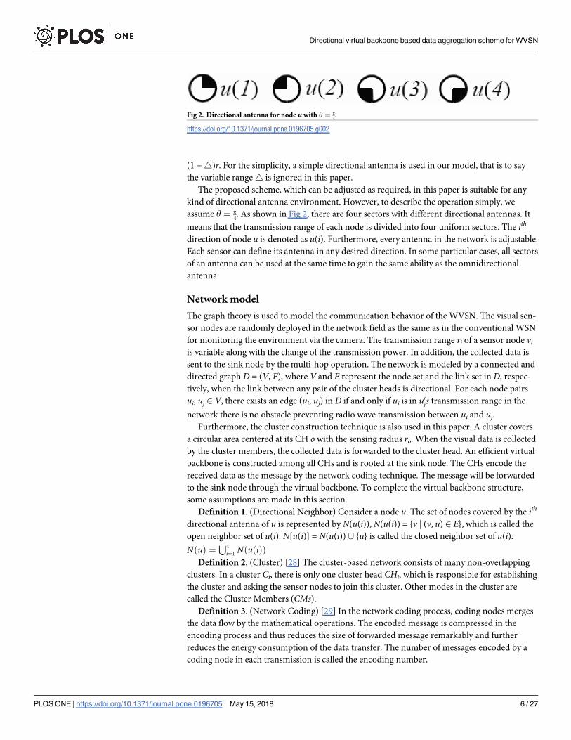
(1 +4)r. For the simplicity, a simple directional antenna is used in our model, that is to say

the variable range4 is ignored in this paper.

The proposed scheme, which can be adjusted as required, in this paper is suitable for any

kind of directional antenna environment. However, to describe the operation simply, we

assume y ¼ p

4. As shown in Fig 2, there are four sectors with different directional antennas. It

means that the transmission range of each node is divided into four uniform sectors. The ith

direction of node u is denoted as u(i). Furthermore, every antenna in the network is adjustable.

Each sensor can define its antenna in any desired direction. In some particular cases, all sectors

of an antenna can be used at the same time to gain the same ability as the omnidirectional

antenna.

Network model

The graph theory is used to model the communication behavior of the WVSN. The visual sen-

sor nodes are randomly deployed in the network field as the same as in the conventional WSN

for monitoring the environment via the camera. The transmission range ri of a sensor node viis variable along with the change of the transmission power. In addition, the collected data is

sent to the sink node by the multi-hop operation. The network is modeled by a connected and

directed graph D = (V, E), where V and E represent the node set and the link set in D, respec-

tively, when the link between any pair of the cluster heads is directional. For each node pairs

ui, uj 2 V, there exists an edge (ui, uj) in D if and only if ui is in u0js transmission range in the

network there is no obstacle preventing radio wave transmission between ui and uj.

Furthermore, the cluster construction technique is also used in this paper. A cluster covers

a circular area centered at its CH o with the sensing radius ro. When the visual data is collected

by the cluster members, the collected data is forwarded to the cluster head. An efficient virtual

backbone is constructed among all CHs and is rooted at the sink node. The CHs encode the

received data as the message by the network coding technique. The message will be forwarded

to the sink node through the virtual backbone. To complete the virtual backbone structure,

some assumptions are made in this section.

Definition 1. (Directional Neighbor) Consider a node u. The set of nodes covered by the ith

directional antenna of u is represented by N(u(i)), N(u(i)) = {v j (v, u) 2 E}, which is called the

open neighbor set of u(i). N[u(i)] = N(u(i)) [ {u} is called the closed neighbor set of u(i).NðuÞ ¼

S4

i¼1NðuðiÞÞ

Definition 2. (Cluster) [28] The cluster-based network consists of many non-overlapping

clusters. In a cluster Ci, there is only one cluster head CHi, which is responsible for establishing

the cluster and asking the sensor nodes to join this cluster. Other modes in the cluster are

called the Cluster Members (CMs).Definition 3. (Network Coding) [29] In the network coding process, coding nodes merges

the data flow by the mathematical operations. The encoded message is compressed in the

encoding process and thus reduces the size of forwarded message remarkably and further

reduces the energy consumption of the data transfer. The number of messages encoded by a

coding node in each transmission is called the encoding number.

Fig 2. Directional antenna for node u with y ¼ p

4.






In this paper, the CHs are all equipped with the ability to be the coding nodes. Since the CH

is taking the responsibility of collecting data of its cluster and encoding the received data

before transmission, the energy consumption of the CH is naturally larger than the ordinary

nodes. The energy consumption model is introduced in the next subsection.

Energy consumption model

The energy consumption is directly related to the size of the transmitted packet k and the

transmission distance d between the transmitter and the receiver nodes. We use the multi-path

fading channel models as in [10, 30], which are shown in the Formulas (1) and (2):

ETxðk; dÞ ¼ Eelec � kþ Efs � k � d2ðd < dtrÞ ð1Þ

ETxðk; dÞ ¼ Eelec � kþ Emp � k � d4ðd � dtrÞ ð2Þ

where Eelec(nJ/bit) is the electronics energy, Efs(pJ/bit/m2) and Emp(pJ/bit/m2) are the energy

amplifier coefficients that depends on the distance to the receiver, and dtr is a distance thresh-

old between the transmitter.

The consumed energy for receiving a packet can be formulated by Formula (3):

ERx ¼ Eelec � k ð3Þ

Definition 4. (Data Generation Rate) The data generation rate Rgi is defined as the amount

of data generated by sensor vi in a data collection round.

Definition 5. (Data Reception Rate) The data reception rate RrCHi

of CHi is defined as the

amount of data CHi receives from its children in a data collection round.

Definition 6. (Transmission Rate) The transmission rate RtCHi

of CHi is the amount of data

transmitted by the cluster head CHi in a data collection round as well.

Definition 7. (Energy Loss Rate) The energy loss rate of the cluster head CHi is given by:

ECHi¼ Rt

CHiETx þ Rr

CHiERx: ð4Þ

Definition 8. (Energy Consumption Density) The energy consumption density DeCHiis a

metric for the load balance, which is the rate between the intra-cluster energy consumption

ECHiand the area of the region the cluster head covered SCHi

.

Definition 9. (Node lifetime) The load LCHiof a cluster head CHi is defined as the ratio of

ECHito the energy it maintains EMCHi

. The lifetime of a cluster head is given by:

TCHi¼ EMCHi

=ECHi¼ 1=LCHi

: ð5Þ

Definition 10. (Network Lifetime) The lifetime of a network is defined as the lifetime of the

virtual backbone lifetime time TVB, which is the minimum lifetime of all nodes in VB. For-

mally,

TVB ¼ minfTCHijCHi 2 VBg: ð6Þ

Network coding and clustering-based data aggregation scheme

Clustering and network coding is essential to remove the redundancy and reduce the size of

the data. In the proposed Directional Virtual Backbone based Data Aggregation Scheme

(DVBDAS) for the WVSNs, the CHs collect data from their own clusters and encode the data




into message packets before forwarding the packets to the sink node via the virtual backbone

data aggregation tree. The DVBDAS is composed of three procedures:

(1) Cluster construction: Through the cluster construction process, the whole network cov-

erage area can be treated as the union of sets composed of clusters.

(2) Directional virtual backboard construction: Constructing an efficient directional virtual

backbone for transmitting the visual data back to the sink node.

(3) Network coding by the CHs.

Cluster construction

The cluster construction aims to the whole network coverage area into several clusters. It can

be divided into 4 steps: the network configuration, the cluster centroid initialization, the load

balance-based CH selection, and the CH update.

Step 1 (Network Configuration): Since multi-hop strategy is used in the data forwarding

mechanism, the energy consumption of CHs nearby the sink node would be higher than the

others because more packets need to be forwarded by them. In order to balance the regional

energy consumption, the regional autonomy method is used in this algorithm. Every region

has a CH selection probability, that is to say sensors in this region become a CH with probabil-

ity pi, which is determined by the distance to the sink node and the network density.

Once sensor nodes are deployed in the network field, they have the information about their

relative coordinates. Driven by a hand-shake mechanism, the sensor node sends packet con-

taining its sensing range ri, the sensor ID, the union set of the neighborhoods N(ui), and the

directional antenna to the Sink Dirs in the network as the “hello message” to its neighbors at

the beginning. The hello message is defined as:

hello message ¼ fri; ID;NðuiÞ;Dirsg: ð7Þ

Step 2 (Cluster Centroid Initialization): To initialize the clustering algorithm, sensor

nodes from the candidate list are randomly selected to be the initial CHs. A sensor node, of

which the current energy Ei is equal to or greater than a predefined threshold ETH is eligible to

be selected as the CH. Thus, all sensor nodes can be classified into two possible cases listed as

follows.

Case 1: (Ei< ETh): The current energy level of the sensor node is lower than the threshold

and thus it can not be selected as the CH. The node is marked as a normal node and is

excluded from the candidate list.

Case 2: (Ei� ETh): The sensor node has sufficient energy and it is collected in the candidate

list. The probability of choosing this sensor node to be the CH is denoted by pi. If a node is

selected to be the CH, it broadcasts a packet called “candidate message” to the others with the

content of the Maintained Energy EMi, a union set of its neighborhoods N(ui), and its ID. The

candidate message can be defined by Formula (8):

CH candidate message ¼ fEi;NðuiÞ; IDg: ð8Þ

Step 3 (Load balance-based CHs Selection): In the previous step, the CHs are initially

selected based on the energy levels. To optimize the selected CHs, the load balance needs to be

taken into account for selecting the CHs because the ideal case is that the energy consumption

of all CHs can be unified. According to Definition 7, the energy consumption of a CH with its

members are physically located far away from it could be higher than a CH with more mem-

bers but located nearby it. It implies that considering only the density of the cluster member is

not sufficient. Thus, we define the energy consumption density Dec to present the rate between

the intra-cluster energy consumption and the region the cluster head covered defined in




Definition 8 and use it as the factor for the consideration. The load of CHs would be more bal-

anced when Dec is involved in the decision. The optimal number of the CHs is defined as fol-

lows:

Nopt ¼ a1

1

Decþ a2EMi þ a3

NðuiÞ

Sarea: ð9Þ

where Nopt denotes the optimal number of the CHs, α1, α2 and α3 (α1 + α2 + α3 = 1) are the

influence factors that can be put with different weights based on the needs.

The Nopt is emphasized by the fact that the energy consumption is well distributed over the

clusters. Nopt is higher when the remained energy of the CH is higher. If there is a neighbor

node v whose optimal number is higher than u, then v will be selected as a cluster head and the

CH message will be broadcasted by it.

The sensor node is merged into a cluster once it receives the CH candidate message. If a

node receives more than one CH candidate message (such as that the node v’s neighbor CH

Nch[v]> 1), it is merged into the cluster, of which the CH is physically the nearest to it. In

order to estimate the efficiency of the algorithm, a data aggregation level network based load

balance factor is assumed. In the data aggregation application, “funneling effect” may be

appeared in the several-to-one data flow network. It means that the load of nodes nearby the

sink node is greater than the others. Hence, the distance between the sink node and the CH is

used as the weight of the original load. The weighted load is defined as Li = li × di. Assume

there are n CHs, of which the weighted loads are denoted by L1, L2, . . ., Ln and all weighted

loads are greater than 0. Since the data aggregation is a constant, we have L1 + L2 + . . . +

Ln = C, where C is the data aggregation constant. According to the in-equation theory, there is

s ¼ðPn

i¼1LiÞ

2

nPn

i¼1L2

i

� 1; ð10Þ

where σ is the load balance factor denoting the load balance level. The load balance is much

greater when σ is approaching to 1. Especially, when L1 = L2 = . . . = Ln, the left side of the in-

equation will achieve the maximum value. In other words, the load balance is achieved. Based

on these three steps, the cluster construction algorithm is shown in Algorithm 1.

Algorithm 1: Cluster Construction

1 with probability pi, each node broadcasts hello message = {ri, ID, N(ui), Dirs};2 if (Ei � ETh) then3 who wants to become a candidate cluster head will broadcasts the‘candidate cluster head’ message: CH candidata message = {Ei, N(ui),ID};4 end5 its neighbor whose optimal number Nopt is higher than the candidatecluster head, it will be the cluster head;6 broadcasts the ‘cluster head’ message;7 calculates the load balance factor;8 if (σ < TRσ) then9 cluster head reselect;10 end11 those who receive the cluster head broadcast message can decided tobe the cluster head’s cluster member;




An example is shown in Figs 3 and 4. Fig 3 shows an original network, visual sensors are

disposed in the area interested. In this example, the interested area is a rectangle. The sink

node is in the front of the rectangle. After step 2 (lines 1-4 in Algorithm 1.), each sensor is

assigned to a specific CH. However, the cluster’s size may exert an effect on the energy con-

sumption and the load. A cluster, of which includes more cluster members or the distances

between cluster members to the CH is greater, may endure heaver load than others with less

cluster members or with more compact cluster structure. Thus, an adapted cluster construc-

tion is given (lines 5-10 in Algorithm 1). After applying Algorithm 1, the clusters are con-

structed as shown in Fig 4.

Step 4 (CH Update): When a CH dies in a cluster, it does not mean that this cluster is use-

less. To balance the energy consumption inside the network, the role of the CH is shifting

among all sensor nodes in the same cluster. The CH reselection will be applied in the cluster

Fig 3. An origin wireless visual sensor network.






when the CH find its energy is not enough for maintaining the cluster. The algorithm is similar

to the Algorithm 1. The sensor node, which has not been selected to be the CH for a long

period has greater chance to be selected as the replacement of the CH. The network lifetime is

defined in Formula (11):

T ¼ minfTCijCi is a clusterg: ð11Þ

Directional virtual backboard construction

After the clusters are constructed, the visual data should be transmitted to the sink node by a

directional virtual backbone. This section will introduce how to construct an efficient direc-

tional virtual backbone between CHs and the sink node. In the omnidirectional antenna

Fig 4. Cluster construction and cluster head selection.






environment, sending signals to some directions are unnecessary because there is no receivers

on those sectors, which is shown in Fig 5(a). In order to avoid the energy consumption on the

unnecessary directions, the directional antennal shown in Fig 5(b) can be used to achieve the

goal. By transmitting packets to only the necessary sectors, the WVSN shown in Fig 5(c) can

preserve more energy in the transformation progress because the antennas on the unused

directions can be turned off.

Algorithm 2: Directional virtual backboard construction

1 Each CH searches open the directional antenna ni, which is toward thedirection of the sink node;2 if (CHi’s radius ri � rtr and there is one neighbor CHj exist) then3 add this link into the edge E(i ! j);4 end5 else6 if (one CHi’s radius ri � rtr and there is no neighbor CH exist)then7 expend the radius energy until find one neighbor CH;8 end9 else10 while (k < = 4) do11 {close directional antenna ni;12 open the nj = ++ni(mod 4) directional antenna;13 operate steps 2-8;14 record the founded parents CHj(nj);}15 end16 end17 end18 compare each d(CHi, CHj(nj)});19 record dmin(j) = min{d(CHi, CHj(nj)})} j = 1, 2, 3, 4; then CHj isCHi’s parents CH;

The constructed directional virtual backbone looks like a directional tree. The sink node is

the root of the directional virtual backbone tree T at level 0. In the tree, nodes CHi and CHj are

siblings when they share the same parents. The set of children of CHi is denoted by Childi.

There can be different paths from a cluster head CHi to the root in different data collection

trees of GCH. Algorithm 2 describes the directional virtual backboard construction algorithm

Fig 5. The omni-antenna graph and direction antenna graph.






in detail. The CHs should find their parents CHs toward the direction of the sink node within

the radius (lines 1-8 in Algorithm 2). If CH parents selection is fall in this direction, the subop-

timum directional antenna will be selected by opening the directional antennas in turn (lines

10-15 in Algorithm 2). The directional to the sink node and nearest CH (lines 18-19 in Algo-

rithm 2) will be chosen as the parents.

An example is shown in Figs 6 (by direction antenna) and Fig 7 (by omni-antenna). It is

easy to find that about 15

36direction antennas (where 15 is the number of the used directional

antennas, and the total number of directional antennas is 9 × 4) are used comparing to the vir-

tual backboard construction by omnidirectional antenna. Without special circumstances, Fig 8

shows another situation, where the sink is in the center. It is easy to find that only 22 direction

antennas are used (total number of directional antennas is 15 × 4), almost 60% CH’s energy

can be safety comparing to virtual backboard construction by omnidirectional antenna.

Fig 6. Directional virtual backboard construction.






Network coding

The WVSN’s natural property of easy packet loss, which makes it a challenge to transmit infor-

mation. Network coding is an efficient solution. There are many kinds of network coding algo-

rithms, the random linear network coding and decoding algorithms [29, 31] will be used in

this paper. Each source node sends out a data packet of length n0 symbols. We consider a set of

packets u1; u2; :::; uK 2 F1�n0q . A coded packet is formed by [gx], where x ¼

PKk¼1

gkuk is a linear

combination of the data packets and g = [g1, g2, . . ., gK] is the global encoding vector for that

packet. At the sink, N packets are received, which can be represented by Formulas (12)

Fig 7. Virtual backboard construction by omni-antenna.






and (13):

X ¼

x1

:::xK

2

664

3

775

T

¼ GU 2 FK�n0q ð12Þ

U ¼

u1

:::uK

2

664

3

775

T

;G ¼

g1

:::gK

2

664

3

775

T

2 FK�Kq ð13Þ

Fig 8. Sink in the center.






The network coding algorithm is applied at coding nodes. In this scheme, the cluster heads

are defined as the coding nodes. The network encoding algorithm is described in Algorithm 3.

All the necessary linear operations are performed over the finite field F28 (lines 9-12 in Algo-

rithm 3). The cluster head codes the messages, which are received from its cluster members,

into one coded packet. Before this coding progress, the cluster head will judge the data’s

repeatability (lines 3-7 in Algorithm 3). Repetitive messages will be discarded.

Algorithm 3: network encoding algorithm

1 set a random counting down time t;2 if (some messages are received) then3 check whether there are same message;4 if (there are some similar message) then5 only chose one message from them;6 set en = number of messages;7 end8 end9 for (j = 1;j < = en;j++) do10 Select en coefficients Ci, i = 1, 2, . . ., en from GF(28) randomly;11 generates new encoded packets by encoding the en data messages Digiven by X ¼

Peni¼1

CiDi;12 broadcast the encoded packets X;13 end

The decoding progress starts when the CH receives the encoded packets. If the decoding

progress is unsuccessful, some packets need to be retransmitted. Let RP refers to the number

of encoded packets the considered node need to send out. RP = en − rank(Cn), each node

sends out a RP of encoded packets. We call it the negative ACK message. Nodes receiving less

than en packets can send out NACK message to some particular neighbors to retrieve missing

data that they need. The nodes that have received NACK message send out RP encoded pack-

ets. This improved encoding algorithm with NACK is described as follows.

Algorithm 4: network decoding algorithm

1 set RP = en − rank(Cn);2 if (RP > 0) then3 require another S encoded packets;4 sent S NACKs to the child CH;5 end6 Restart the countdown t;7 receive the packets;8 decoding the packets;

When the decoding node receives the encoded packets from cluster heads in the upstream,

the countdown will begin. If the received packet can be successfully decoded in t time slots, the

information is combined with their own information, and then forward to the next layer. If

the decoding is unsuccessful, the coding node needs to calculate the value of RP and send the

RP NACKs to the child CH and restart the countdown when receiving the encoded packet,

next time. If it can be decoded within t times, then the encoding packages will be forward to

the next layer. Otherwise goto this step till the encoding packet can be decoded successful. If

the encoding node receives the NACK from the next layer cluster head, execution the next

stage. The network decoding algorithm is described in Algorithm 4.




Theoretical analysis

The performances of our scheme will be studied in this section. Derived in Theorem 1, the

energy consumption of the proposed method is lower than other methods. The boundary of

the network lifetime is given in Theorems 2 and 3.

Theorem 1: The energy consumption by the scheme is about N � ð1 � paverÞ �ð

d 1

pavere � 1

� �� a2

2p�N�paver� Efs þ Eelec

� �þ N � paver � ðriÞ

2� Efs � kþ Eelec � kÞ � pdi, which is

smaller than other omni-directional antennal scheme.

Proof: Assume the average transmit radius rave is:

rave ¼a

ffiffiffiffiffiffiffiffiffiffiffiffiffiffiffiffiffiffiffiN � paverpp : ð14Þ

where a is the length of the network area, N is the number of total sensor planted in the net-

work, paver is the average probability of the cluster head selection.

Assume CHi is a cluster head whose average radius is ri, and ρ(CHi) is the sensor node dis-

tribution density function for the cluster form by node CHi, then the expectation of the dis-

tance between cluster member and cluster head can be calculated as:

Eðd2ðn; jÞÞ ¼Z Z

CHi

� ðx2 þ y2Þ � rðCHiÞd areaðCHiÞ

¼

Z 2p

0

Z rave

0

r3 Npaver

a2drdy

¼a

2pNpaver

ð15Þ

This density function is in the trend of the uniform distribution, which is approximately

equal toNpavera2 .

The transmit and the receive energy consumption is presented in Formulas (1–3). The total

energy consumption is contained by two aspects, the intra-cluster energy consumption and

the inter-clusters energy consumption. According to the density function and the consump-

tion model, then the energy consumption of the intra-cluster can be calculated as:

Eðj; nÞ ¼XNeðCHiÞ

j¼1

d2ðj; nÞ � Efs þ NeðnÞ � Eelec ð16Þ

where, Ne(CHi) is the number of the cluster head CHi’s neighbors. If the nodes are uniformly

distributed in the cluster, the expectation of the energy consumption of the intra-cluster is:

Eðj; nÞ ¼ N � ð1 � paverÞ �1

paver

� �

� 1

� �

�a2

2pNpaver� Efs þ Eelec

� � ð17Þ

The expectation distance between the CHs and the sink node is:

EðdðCHi; sinkÞÞ ¼Z a

2

� a2

Z a2

� a2

ffiffiffiffiffiffiffiffiffiffiffiffiffiffix2 þ y2

p� r2ðnÞdxdy

¼R a

2

� a2

ffiffiffiffiffiffiffiffiffiffiffiffiffiffix2 þ y2

p�

1

a2dxdy ¼ 0:3825a

ð18Þ




where ρ(CHi) is the cluster heads distribution density. Assume the nodes are uniform distribu-

tion in the a × a area. Then the expectation energy consumption by the CHs is:

Eðn; sÞ ¼ N � paver � ½ðriÞ2� Efs � kþ Eelec � k� ð19Þ

If not use multi-hop routing, the expectation energy consumption by the CHs is:

Eðn; sÞ ¼ N � paver � ½ð0:3825aÞ2 � Efs � kþ Eelec � k� ð20Þ

which is more than our scheme. Then the total energy consumption is:

ðN � ð1 � paverÞ �1

paver

� �

� 1

� �

�� a2

2p � N � paver� Efs

þ Eelec

�þ N � paver � ðriÞ

2� Efs � kþ Eelec � kÞ � pdi:

ð21Þ

where pdi is the directional probability.

Theorem 2: If VBi is an optimally balanced virtual backbone tree, its lifetime t(VBi) is the

lifetime of the WVSNs.

Proof: Assume that VBi is an optimally balanced virtual backbone tree and some non-opti-

mal tree VBj provides the maximum lifetime. According to Formula (7), let VBj be σj-balanced

and VBi be σi-balanced, where σi� σj. Let CHx lie on the balanced virtual backbone tree VBi

and who has the largest load. According to Definition 10, the network lifetime is t(VBi) = t(CHx). Since CHx has the least lifetime in VBi, the load LCHx

of CHx is the maximum along the

virtual backbone tree VBi.

Also, let CHy have the largest load in VBj. Similarly, we have t(VBi) = t(CHy). By definition,

LCHy= σj, LCHx

= σi. In more balanced virtual backbone tree, each CH’s load is more equivalent,

and thus there is LCHx> LCHy

and σi� σj. Hence, VBi provides the maximum lifetime for the

network.

Theorem 3. Based on the DVBDAS scheme, the upper bound network lifetime is:

maxT ¼E0

RtCHi

ETx þ RrCHi

ERx� Npaver: ð22Þ

Proof: The virtual backbone tree VBi is active in the interval ½Pi� 1

j¼0tj;Pi

j¼0tj�, the whole net-

work will die when the energy of one cluster’member are all exhausted. According to

Formula (11), the lifetime of a schedule is defined as T = min{TCi|Ci is the cluster}.

Assume that E0 is the initial energy for each node. According to Formulas (1–5), the lifetime

of u can be expressed as:

tu ¼E0

RtCHi

ETx þ RrCHi

ERx: ð23Þ

Assume that paver is the average probability for selecting the CH at each location. The size of

the cluster is given as Npaver. The lifetime can be presented as:

maxT ¼E0

RtCHi

ETx þ RrCHi

ERx� Npaver: ð24Þ




Simulation

In this section, we will compare our DVBDAS scheme with the normal routing algorithm

without clustering and the scheme based on the cluster with omnidirectional antennas. The

data generation rate Rgi of every node is calculated in a sensing and reporting cycle. In order to

simulate the reality in the real-world scenario, we assume that the probability rate pi ¼ Rgi is

depended by the area, which fits in a multi-peak Gaussian Distribution. It can be described by

Formula (25), which is constructed in our previous work [32]. The simulation results are pre-

sented with the average values.

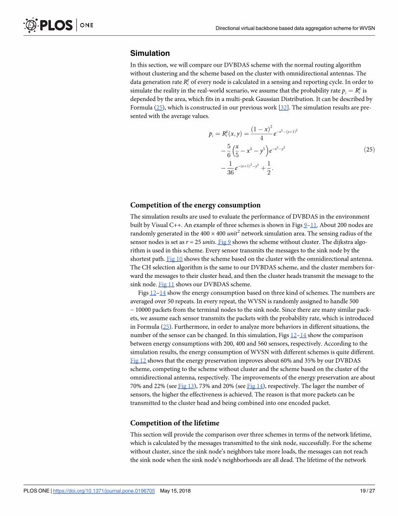
pi ¼ Rgi ðx; yÞ ¼

ð1 � xÞ2

4e� x2 � ðyþ1Þ2

�5

6

x5� x3 � y5

� �e� x2 � y2

�1

36e� ðxþ1Þ2 � y2

þ1

2:

ð25Þ

Competition of the energy consumption

The simulation results are used to evaluate the performance of DVBDAS in the environment

built by Visual C++. An example of three schemes is shown in Figs 9–11. About 200 nodes are

randomly generated in the 400 × 400 unit2 network simulation area. The sensing radius of the

sensor nodes is set as r = 25 units. Fig 9 shows the scheme without cluster. The dijkstra algo-

rithm is used in this scheme. Every sensor transmits the messages to the sink node by the

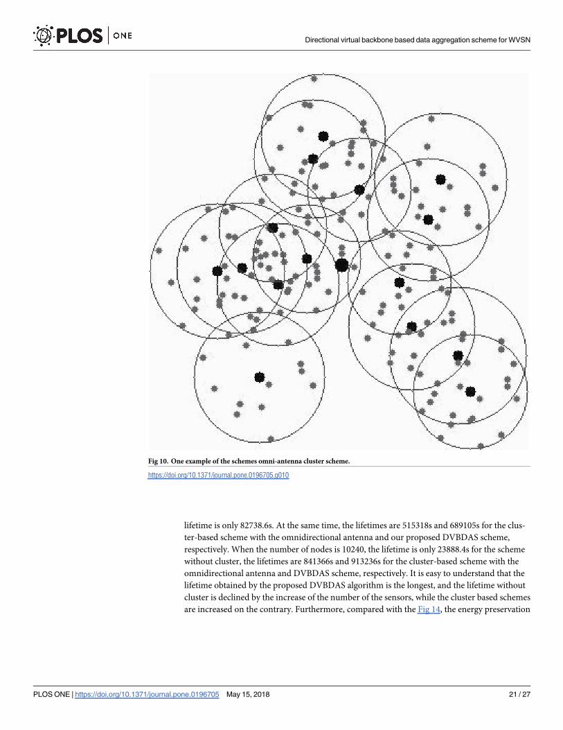
shortest path. Fig 10 shows the scheme based on the cluster with the omnidirectional antenna.

The CH selection algorithm is the same to our DVBDAS scheme, and the cluster members for-

ward the messages to their cluster head, and then the cluster heads transmit the message to the

sink node. Fig 11 shows our DVBDAS scheme.

Figs 12–14 show the energy consumption based on three kind of schemes. The numbers are

averaged over 50 repeats. In every repeat, the WVSN is randomly assigned to handle 500

− 10000 packets from the terminal nodes to the sink node. Since there are many similar pack-

ets, we assume each sensor transmits the packets with the probability rate, which is introduced

in Formula (25). Furthermore, in order to analyze more behaviors in different situations, the

number of the sensor can be changed. In this simulation, Figs 12–14 show the comparison

between energy consumptions with 200, 400 and 560 sensors, respectively. According to the

simulation results, the energy consumption of WVSN with different schemes is quite different.

Fig 12 shows that the energy preservation improves about 60% and 35% by our DVBDAS

scheme, competing to the scheme without cluster and the scheme based on the cluster of the

omnidirectional antenna, respectively. The improvements of the energy preservation are about

70% and 22% (see Fig 13), 73% and 20% (see Fig 14), respectively. The lager the number of

sensors, the higher the effectiveness is achieved. The reason is that more packets can be

transmitted to the cluster head and being combined into one encoded packet.

Competition of the lifetime

This section will provide the comparison over three schemes in terms of the network lifetime,

which is calculated by the messages transmitted to the sink node, successfully. For the scheme

without cluster, since the sink node’s neighbors take more loads, the messages can not reach

the sink node when the sink node’s neighborhoods are all dead. The lifetime of the network




ends when all neighbors of the sink node are dead. The lifetime of the cluster based scheme

ends when there is no CH can be selected in a cluster for transmitting the messages.

Sensors are also deployed in a 400�400 unit2 area. The sensing range is fixed to 25. The

transmit range is adjustable. The initial node battery capacity is 2500 mAh, the transmission

power is 60mW, the receiving power is 45mW. The number of nodes is risen from 2730 to

10240. Fig 15 shows the lifetime of different schemes in such case. The lifetime obtained by the

scheme without cluster is the shortest. For example, when the number of nodes is 2730, the

Fig 9. One example of the schemes without cluster.






lifetime is only 82738.6s. At the same time, the lifetimes are 515318s and 689105s for the clus-

ter-based scheme with the omnidirectional antenna and our proposed DVBDAS scheme,

respectively. When the number of nodes is 10240, the lifetime is only 23888.4s for the scheme

without cluster, the lifetimes are 841366s and 913236s for the cluster-based scheme with the

omnidirectional antenna and DVBDAS scheme, respectively. It is easy to understand that the

lifetime obtained by the proposed DVBDAS algorithm is the longest, and the lifetime without

cluster is declined by the increase of the number of the sensors, while the cluster based schemes

are increased on the contrary. Furthermore, compared with the Fig 14, the energy preservation

Fig 10. One example of the schemes omni-antenna cluster scheme.






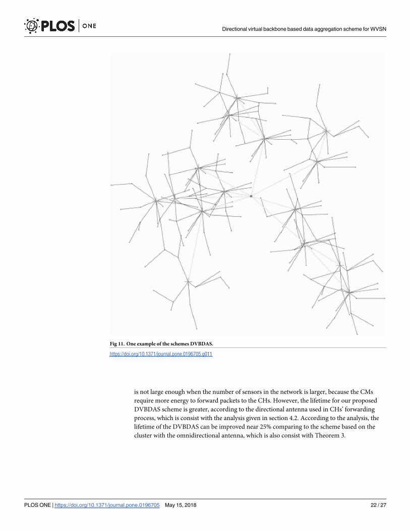
is not large enough when the number of sensors in the network is larger, because the CMs

require more energy to forward packets to the CHs. However, the lifetime for our proposed

DVBDAS scheme is greater, according to the directional antenna used in CHs’ forwarding

process, which is consist with the analysis given in section 4.2. According to the analysis, the

lifetime of the DVBDAS can be improved near 25% comparing to the scheme based on the

cluster with the omnidirectional antenna, which is also consist with Theorem 3.

Fig 11. One example of the schemes DVBDAS.






Fig 12. Comparison for energy consumption in 200 sensors.











Fig 15. The comparison of lifetime.







Conclusion

Data gathering is a fundamental task in WVSNs. Directional antennas have a number of

advantages over omnidirectional antennas. By focusing energy only in the intended direction,

directional antenna can increase the potential for spatial reuse and can provide longer trans-

mission/reception ranges by consuming the same amount of energy. The feature of the direc-

tional antennas and the visual data make WVSNs more complex. Therefore, in this paper, we

focus on constructing a Directional Virtual Backbone based Data Aggregation Scheme

(DVBDAS), which can obtain the minimum energy consumption and maximum network life-

time by combining the cluster algorithm, the directional virtual backbone construction algo-

rithm and the network coding mechanism. Finally, the performances of our proposed

DVBDAS are studied by the theoretical analysis and the simulations. The results indicate that

the energy consumption by the proposed DVBDAS is smaller than other schemes but the net-

work lifetime is longer than others.

Tracking the moving target is considered as one of the important applications in WVSNs.

To the best of our knowledge, improving the tracking quality and extending the network life-

span are two main objects for the target tracking, which are usually contradictory due to lim-

ited energy of sensor nodes in WVSNs. However, the lifetime and the tracking quality also are

two contradictory issues. In the future, we will focus on finding the balance of these two signif-

icate problems.

Supporting information

S1 Fig. One example of the schemes without cluster.

(PDF)

S2 Fig. One example of the schemes without cluster omni-antenna cluster scheme.

(PDF)

S3 Fig. One example of the schemes without cluster DVBDAS.

(PDF)

S1 File. Data. Relevant data underlying the findings described in manuscript.

(ZIP)

Author Contributions

Conceptualization: Jing Zhang.

Data curation: Jing Zhang, Shi-jian Liu, Fu-min Zou, Xiao-rong Ji.

Formal analysis: Jing Zhang, Pei-Wei Tsai.

Funding acquisition: Jing Zhang.

Investigation: Jing Zhang.

Methodology: Jing Zhang.

Project administration: Jing Zhang.

Resources: Jing Zhang.

Software: Jing Zhang.

Supervision: Jing Zhang.



http://www.plosone.org/article/fetchSingleRepresentation.action?uri=info:doi/10.1371/journal.pone.0196705.s001





Validation: Jing Zhang.

Visualization: Jing Zhang.

Writing – original draft: Jing Zhang.

Writing – review & editing: Shi-jian Liu, Fu-min Zou, Xiao-rong Ji.

References1. Li C, Zou J, Xiong H, and Chen CW. Joint coding/routing optimization for distributed video sources in

wireless visual sensor networks. IEEE Transactions on Circuits and Systems for Video Technology.

2011; 21(2): 141–155. https://doi.org/10.1109/TCSVT.2011.2105596

2. Zhou Z, Wu QJ, Huang F, and Sun X. Fast and accurate near-duplicate image elimination for visual sen-

sor networks. International Journal of Distributed Sensor Networks. 2017; 13(2): 1–12. https://doi.org/

10.1177/1550147717694172

3. Vlad T, Dmitri M, Yevgeni K, Ioan T, and Jaakko A. Energy Efficient Wireless Sensor Networks Using

Linear-Programming Optimization of the Communication Schedule. Journal of communications and

networks. 2015; 17(2): 184–197 https://doi.org/10.1109/JCN.2015.000032

4. Kim YH, Han YH, Jeong YS, and Park DS. Lifetime maximization considering target coverage and con-

nectivity in directional image/video sensor networks. Journal of Supercomputing. 2013; 65(1): 365–

382. https://doi.org/10.1007/s11227-011-0646-9

5. Ramanathan R, Redi J, Santivanez C, Wiggins D, and Polit S. Ad hoc networking with directional anten-

nas: a complete system solution. IEEE Journal on Selected Areas in Communications. 2005; 23(3):

496–506. https://doi.org/10.1109/JSAC.2004.842556

6. Ma H, Liu Y. On coverage problems of directional sensor networks. In: The first int conf on mobile ad-

hoc and sensor networks. 2005: 721–731.

7. Rahimi M, Baer R, Iroezi O, Garcia J, Warrior J, Estrin D, Srivastava M. Cyclops: in situ image sensing

and interpretation in wireless sensor networks. In: Proc ACM conf embedded networked sensor sys-

tems. 2005.

8. Peng H, Tian Y, Kurths J, Li L, Yang Y, and Wang D. Secure and energy-efficient data transmission sys-

tem based on chaotic compressive sensing in body-to-body networks. IEEE Transactions on Biomedi-

cal Circuits and Systems. 2017; 11(3): 558–573. https://doi.org/10.1109/TBCAS.2017.2665659 PMID:

28489549

9. Yang Y, Peng H, Li L, and Niu X. General theory of security and a study case in internet of things. IEEE

Internet of Things Journal. 2017; 4(2):592–600. https://doi.org/10.1109/JIOT.2016.2597150

10. Heinzelman WR, Chandrakasan A, and Balakrishnan H. Energy-Efficient Communication Protocol for

Wireless Microsensor Networks. Hawaii International Conference on System Sciences, IEEE Computer

Society. 2000; 18: 8020.

11. Heinzelman WB, Chandrakasan AP, Balakrishnan H. An applicationspecific protocol architecture for

wireless microsensor networks. IEEE Transactions on Wireless Communication. 2002; 1(4): 660–670.

https://doi.org/10.1109/TWC.2002.804190

12. Younis O, Fahamy S. Distributed clustering in Ad-Hoc sensor networks: A hybrid, energy-efficient

approach. in Proc. IEEE INFOCOM. 2004; 1: 629–640.

13. Nayak P, and Devulapalli A. A Fuzzy Logic-Based Clustering Algorithm for WSN to Extend the Network

Lifetime. IEEE SENSORS JOURNAL. 2016; 16(1): 137–144. https://doi.org/10.1109/JSEN.2015.

2472970

14. Hosseini SM, and Kahaei MH. Target detection in cluster based wsn with massive mimo systems. Elec-

tronics Letters. 2016; 53(1): 50–52. https://doi.org/10.1049/el.2016.2563

15. Marappan P, and Rodrigues P. An energy efficient routing protocol for correlated data using cl-leach in

wsn. Wireless Networks. 2016; 22(4): 1–9. https://doi.org/10.1007/s11276-015-1063-4

16. Javed MU. Optimization of leach topology with cost effective deep belief network-hybrid event coverage

in wsn with finite resources. Communications of the Acm. 2016.

17. Liaqat M, Gani A, Anisi MH, Ab Hamid SH, Akhunzada A, and Khan MK. Distance-based and low

energy adaptive clustering protocol for wireless sensor networks. Plos One. 11(9), e0161340. https://

doi.org/10.1371/journal.pone.0161340 PMID: 27658194

18. Farman H, Javed H, Jan B, Ahmad J, Ali S, and Khalil FN. Analytical network process based optimum

cluster head selection in wireless sensor network. Plos One. 2017; 12(7), e0180848. https://doi.org/10.

1371/journal.pone.0180848 PMID: 28719616



https://doi.org/10.1109/TCSVT.2011.2105596

https://doi.org/10.1177/1550147717694172

https://doi.org/10.1177/1550147717694172

https://doi.org/10.1109/JCN.2015.000032

https://doi.org/10.1007/s11227-011-0646-9

https://doi.org/10.1109/JSAC.2004.842556

https://doi.org/10.1109/TBCAS.2017.2665659

http://www.ncbi.nlm.nih.gov/pubmed/28489549

https://doi.org/10.1109/JIOT.2016.2597150

https://doi.org/10.1109/TWC.2002.804190

https://doi.org/10.1109/JSEN.2015.2472970

https://doi.org/10.1109/JSEN.2015.2472970

https://doi.org/10.1049/el.2016.2563

https://doi.org/10.1007/s11276-015-1063-4








19. Almekhlafi ZG, Hanapi ZM, Othman M, and Zukarnain ZA. Travelling wave pulse coupled oscillator

(twpco) using a self-organizing scheme for energy-efficient wireless sensor networks. Plos One. 2017;

12(1), e0167423. https://doi.org/10.1371/journal.pone.0167423

20. Imon SKA, Khan A, Francesco MD, and Das SK. Energy-efficient randomized switching for maximizing

lifetime in tree-based wireless sensor networks. IEEE/ACM Transactions on Networking. 2015; 23(5):

1401–1415. https://doi.org/10.1109/TNET.2014.2331178

21. Kim D, Wu Y, Li Y, Zou F, and Du DZ. Constructing minimum connected dominating sets with bounded

diameters in wireless networks. IEEE Transactions on Parallel and Distributed Systems. 2009; 20(2):

147–157. https://doi.org/10.1109/TPDS.2008.74

22. Yang S, Wu J, and Dai F. Efficient directional network backbone construction in mobile ad hoc net-

works. IEEE Transactions on Parallel and Distributed Systems. 2008; 19(12): 1601–1613. https://doi.

org/10.1109/TPDS.2008.43

23. Ding L, Gao X, Wu W, Lee W, Zhu X, and Du DZ. Distributed construction of connected dominating sets

with minimum routing cost in wireless networks. In Proc. of IEEE ICDCS. 2010.

24. Ding L, Wu W, Willson J, Du H, and Lee W. Efficient virtual backbone construction with routing cost con-

straint in wireless networks using directional antennas. IEEE Transactions on Mobile Computing. 2012;

11(7): 1102–1112. https://doi.org/10.1109/TMC.2011.129

25. Li DQ, Xue WH, Wang HC, and Cau QG. A New Distributed CDS Algorithm of Ad Hoc Network Based

on Weight. International Conference on Intelligent System Design and Engineering Application. 2010;

1: 90–94. https://doi.org/10.1109/ISDEA.2010.235

26. Zhang YJ, Lei L, Zhu G, and Dong T. Distributed neighbor discovery mechanism based on analytical

modeling for ad hoc networks with directional antennas. Journal of Chinese Computer Systems. 2016.

27. Zhang G, Xu Y, Wang X, and Guizani M. Capacity of hybrid wireless networks with directional antenna

and delay constraint. IEEE Transactions on Communications. 2010; 58(7): 2097–2106. https://doi.org/

10.1109/TCOMM.2010.07.090330

28. Abusaimeh H, and Yang SH. Dynamic cluster head for lifetime efficiency in WSN. International Journal

of Automation and Computing. 2009; 6(1): 48. https://doi.org/10.1007/s11633-009-0048-0

29. Vazintari A. Network coding for overhead reduction in delay tolerant networks. Wireless Personal Com-

munications. 2013; 72(4): 2653–2671. https://doi.org/10.1007/s11277-013-1172-2

30. Bouabdallah N, Rivero-Angeles ME, Sericola B. Continuous Monitoring Using Event-Driven Reporting

for Cluster-Based Wireless Sensor Networks. IEEE Transactions on Vehicular Technology. 2009; 58

(7): 3460–3479. https://doi.org/10.1109/TVT.2009.2015330

31. Pfletschinger S, Navarro M, Ibars C. Energy-efficient data collection in WSN with network coding. IEEE

GLOBECOM Workshops. 2011: 394–398.

32. Zhang J, Xu L, Zhou S, and Ye X. A novel sleep scheduling scheme in green wireless sensor networks.

Journal of Supercomputing. 2015; 71(3): 1067–1094. https://doi.org/10.1007/s11227-014-1354-z




https://doi.org/10.1109/TNET.2014.2331178

https://doi.org/10.1109/TPDS.2008.74



https://doi.org/10.1109/TMC.2011.129

https://doi.org/10.1109/ISDEA.2010.235

https://doi.org/10.1109/TCOMM.2010.07.090330

https://doi.org/10.1109/TCOMM.2010.07.090330

https://doi.org/10.1007/s11633-009-0048-0

https://doi.org/10.1007/s11277-013-1172-2

https://doi.org/10.1109/TVT.2009.2015330

https://doi.org/10.1007/s11227-014-1354-z


Documents

Directional virtual backbone based data aggregation scheme