Directed Acyclic Graphs: An Applicationto Modeling Causal Relationships

with Worldwide Poverty Data

Gott würfelt nicht. --Albert Einstein

David A. Bessler

1

David A. BesslerTexas A&M University

Presented toJames S. McDonnell Foundation

21st Century Science Initiative“Creating Knowledge from Information”

Tarrytown, New YorkJune 3, 2003

Outline

� Poverty literature

� Causal modeling and directed graphs

� Directed graphs on poverty variables

2

� Regression, front door, and back door paths

� Summary and caution

� Directed graphs on poverty variables

Food and Agricultural Organization (FAO)of the United Nations

� FAO has the charge to understand the role offood production in poverty alleviation.

� The development literature has identified several variables as being related to poverty.

3

variables as being related to poverty.

� The causal status of many of these variables is unsettled.

� It is unethical to perform random assignment experiments to provide evidence on the causal status of these variables.

A Partial List of Literature on Causes and Effects of Poverty� Agricultural Income (Mellor 2000)

� Freedom (Sachs and Warner 1997)

4

� Income (Sen 1981)

� Income Inequality (Sen 1981)

� Child Mortality (Berhrman and Deolalikar 1988)

Literature Continued� Birth Rate (Malthus 1798; Sen 1981)

� Rural Population (Rosenweig 1988)

� Foreign Aid (World Bank 2000)

5

� Life Expectancy (Wheeler 1980)

� Illiteracy (Birdsall 1988)

� International Trade (Ricardo 1817; Bhagwati 1996)

Measures of PovertyAlternatives are Discussed in Sen:Poverty and Famines, Oxford Press, 1981.

� Economic Measures: e.g., % of Population

Living on One or Two Dollars or Less per Day

6

� Biological Measures: e.g., deficits in

calorie intake

Data Sources

World Bank Development Indicators80 Countries: % of Population Living off of One and Two Dollarsper Day or Less.

7

Heritage FoundationIndex of Economic and Political Freedom on 80 countries.

FAO (United Nations)% of Population that is Under-Nourished.

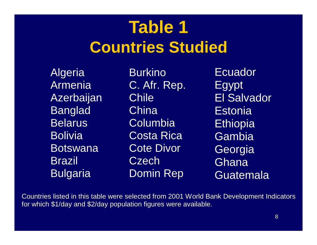
Algeria Armenia Azerbaijan Banglad Belarus

Burkino C. Afr. Rep. Chile China Columbia

Ecuador Egypt El Salvador Estonia Ethiopia

Table 1Countries Studied

8

Belarus Bolivia Botswana Brazil Bulgaria

Columbia Costa Rica Cote Divor Czech Domin Rep

Ethiopia Gambia Georgia Ghana Guatemala

Countries listed in this table were selected from 2001 World Bank Development Indicators for which $1/day and $2/day population figures were available.

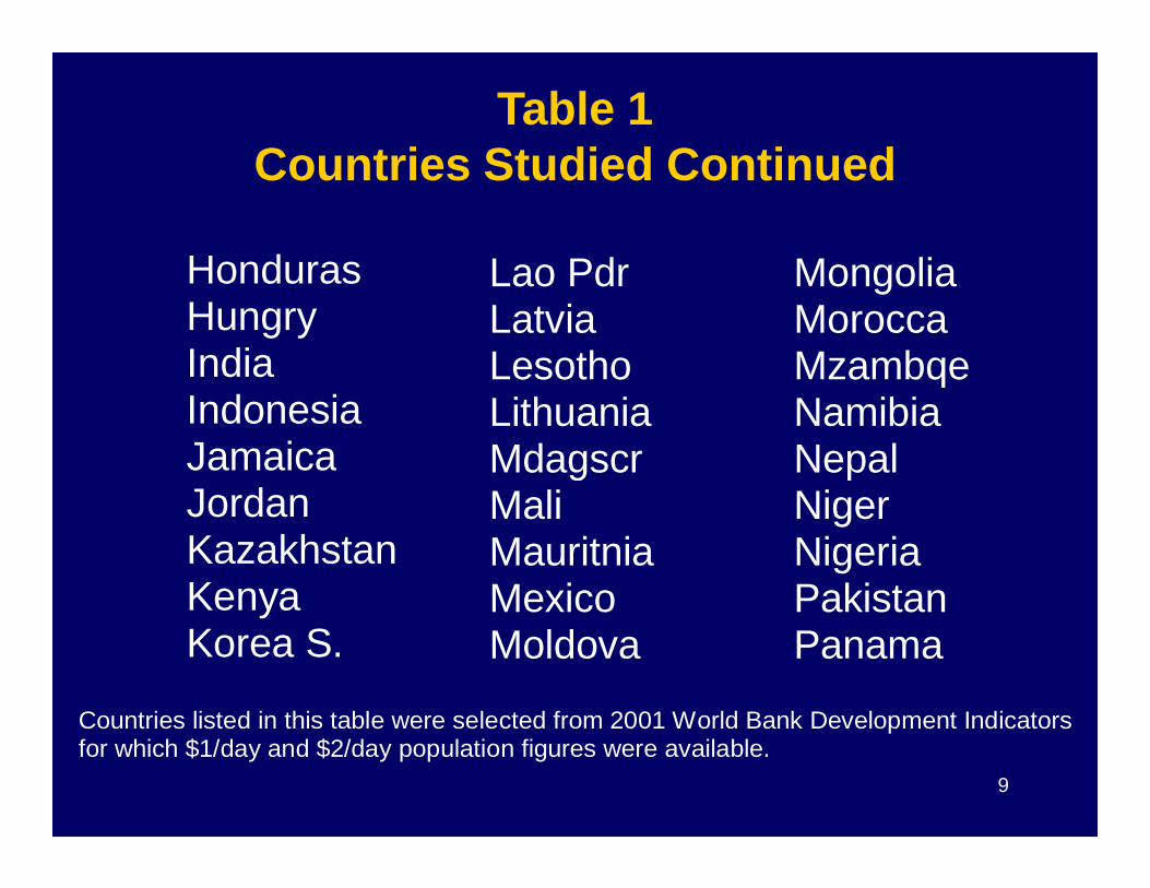
Table 1Countries Studied Continued

Honduras Hungry India Indonesia Jamaica

Lao Pdr Latvia Lesotho Lithuania Mdagscr

Mongolia Morocca Mzambqe Namibia Nepal

9

Jamaica Jordan Kazakhstan Kenya Korea S.

Mdagscr Mali Mauritnia Mexico Moldova

Nepal Niger Nigeria Pakistan Panama

Countries listed in this table were selected from 2001 World Bank Development Indicators for which $1/day and $2/day population figures were available.

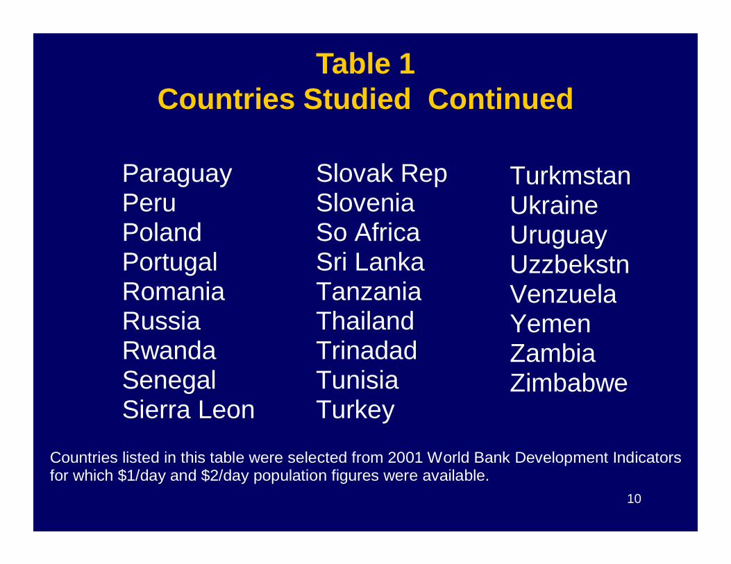
Paraguay Peru Poland Portugal Romania

Slovak Rep Slovenia So Africa Sri Lanka Tanzania

Turkmstan Ukraine Uruguay Uzzbekstn Venzuela

Table 1Countries Studied Continued

10

Romania Russia Rwanda Senegal Sierra Leon

Tanzania Thailand Trinadad Tunisia Turkey

Venzuela Yemen Zambia Zimbabwe

Countries listed in this table were selected from 2001 World Bank Development Indicators for which $1/day and $2/day population figures were available.

Inference on Causal Flows

� Oftentimes we are uncertain about whichvariables are causal in a modeling effort.

11

� Theory may tell us what our fundamentalcausal variables are in a controlled system.

� It is common that our data may not becollected in a controlled environment.

Use of Subject Matter Theory

Theory may be a good source of information about

direction of causal flow among variables. However,theory usually invokes the ceteris paribus condition

to achieve results.

12

to achieve results.

Data are often observational (non-experimental)and thus the ceteris paribus condition may nothold. We may not ever know if it holds becauseof unknown variables operating on our system.

Experimental Methods

� If we do not know the "true" system, but have an idea that one or more variables operate on that system, then experimental methods can yield appropriate results.

13

� Experimental methods work because they use randomization, random assignment of subjects to alternative treatments, to account for any additional variation associated with the unknown variables on the system.

Observational Data

In the case where no experimental control is used in the generation of our data, such data are said to be observational (non-experimental).

14

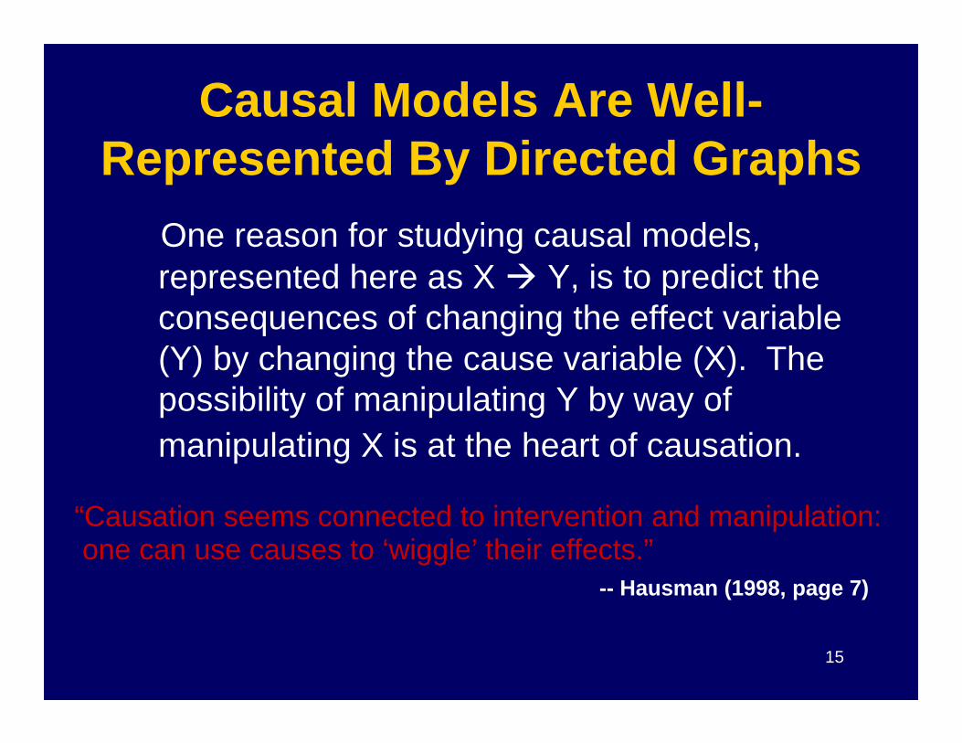
Causal Models Are Well-Represented By Directed Graphs

One reason for studying causal models, represented here as X � Y, is to predict the consequences of changing the effect variable (Y) by changing the cause variable (X). The

15

(Y) by changing the cause variable (X). The possibility of manipulating Y by way of manipulating X is at the heart of causation.

“Causation seems connected to intervention and manipulation:one can use causes to ‘wiggle’ their effects.”

-- Hausman (1998, page 7)

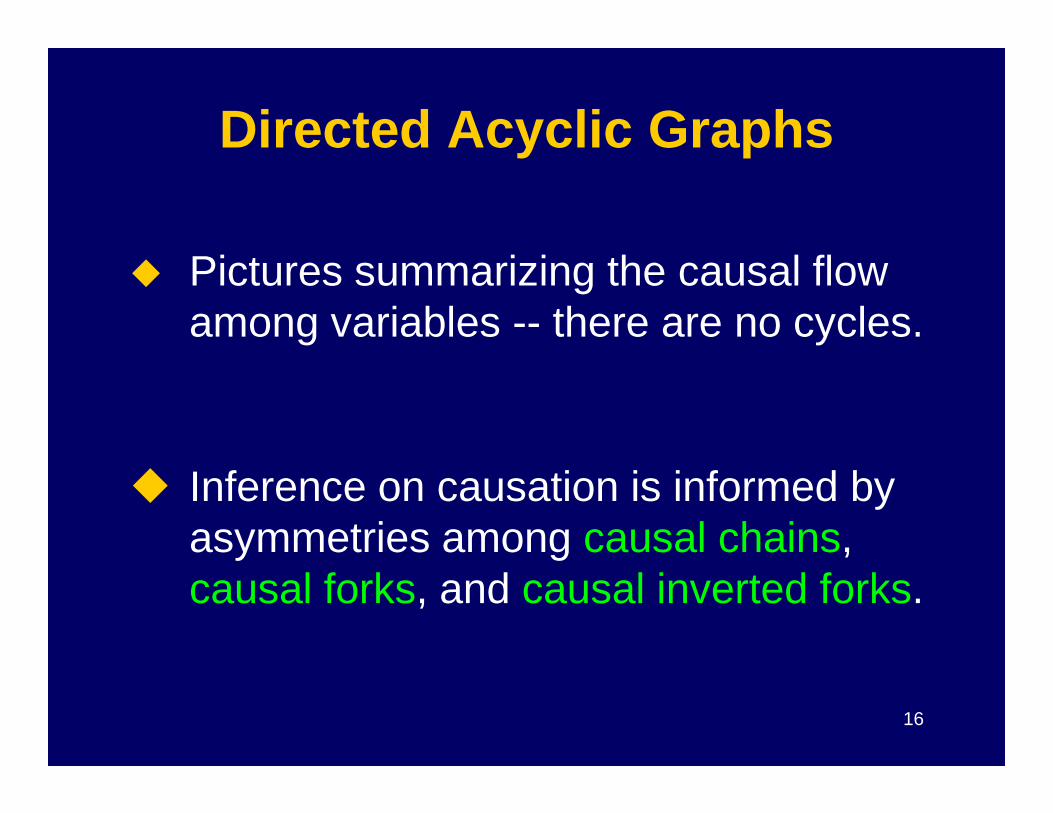
Directed Acyclic Graphs

� Pictures summarizing the causal flow among variables -- there are no cycles.

16

� Inference on causation is informed by asymmetries among causal chains, causal forks, and causal inverted forks.

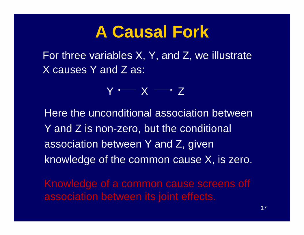
A Causal ForkFor three variables X, Y, and Z, we illustrateX causes Y and Z as:

Here the unconditional association between

X ZY

17

Here the unconditional association betweenY and Z is non-zero, but the conditionalassociation between Y and Z, givenknowledge of the common cause X, is zero.

Knowledge of a common cause screens off association between its joint effects.

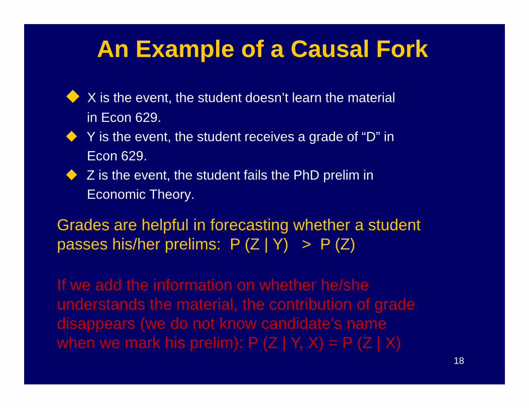
An Example of a Causal Fork

� X is the event, the student doesn’t learn the material

in Econ 629. � Y is the event, the student receives a grade of “D” in

Econ 629.� Z is the event, the student fails the PhD prelim in

Economic Theory.

18

Grades are helpful in forecasting whether a student passes his/her prelims: P (Z | Y) > P (Z)

If we add the information on whether he/she understands the material, the contribution of grade disappears (we do not know candidate’s name when we mark his prelim): P (Z | Y, X) = P (Z | X)

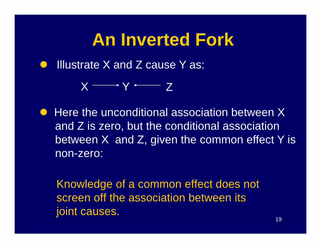
An Inverted Fork

� Here the unconditional association between Xand Z is zero, but the conditional association

� Illustrate X and Z cause Y as:

X Y Z

19

Knowledge of a common effect does not screen off the association between its joint causes.

and Z is zero, but the conditional associationbetween X and Z, given the common effect Y is non-zero:

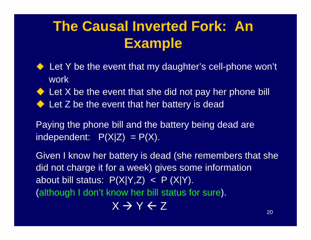
The Causal Inverted Fork: An Example

� Let Y be the event that my daughter’s cell-phone won’t work

� Let X be the event that she did not pay her phone bill� Let Z be the event that her battery is dead

Paying the phone bill and the battery being dead are

20

Paying the phone bill and the battery being dead are independent: P(X|Z) = P(X).

Given I know her battery is dead (she remembers that shedid not charge it for a week) gives some information about bill status: P(X|Y,Z) < P (X|Y).(although I don’t know her bill status for sure).

X � Y Z

The Literature on Such Causal Structures Has Been Advanced in the Last Decade Under the Label of Artificial Intelligence

� Pearl , Biometrika, 1995

� Pearl, Causality, Cambridge Press, 2000

21

� Spirtes, Glymour and Scheines, Causation,Prediction and Search, MIT Press, 2000

� Glymour and Cooper, editors, Computation, Causation and Discovery, MIT Press, 1999

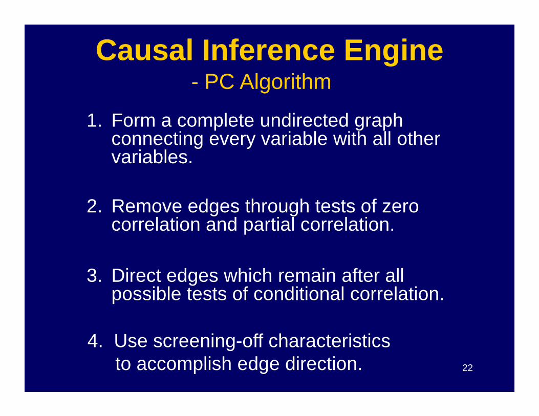
Causal Inference Engine

1. Form a complete undirected graph connecting every variable with all other variables.

2. Remove edges through tests of zero

- PC Algorithm

22

2. Remove edges through tests of zero correlation and partial correlation.

3. Direct edges which remain after all possible tests of conditional correlation.

4. Use screening-off characteristicsto accomplish edge direction.

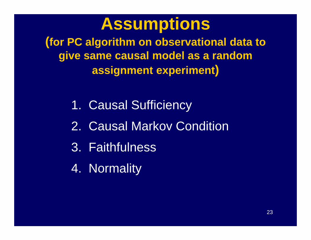
Assumptions(for PC algorithm on observational data to

give same causal model as a random assignment experiment)

1. Causal Sufficiency

2. Causal Markov Condition

23

2. Causal Markov Condition

3. Faithfulness

4. Normality

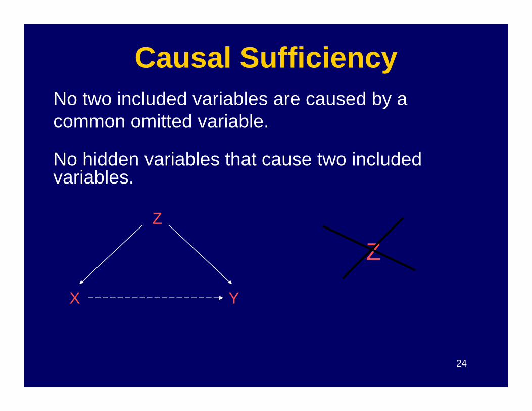
Causal SufficiencyNo two included variables are caused by acommon omitted variable.

No hidden variables that cause two included variables.

24

Z

X Y

Z

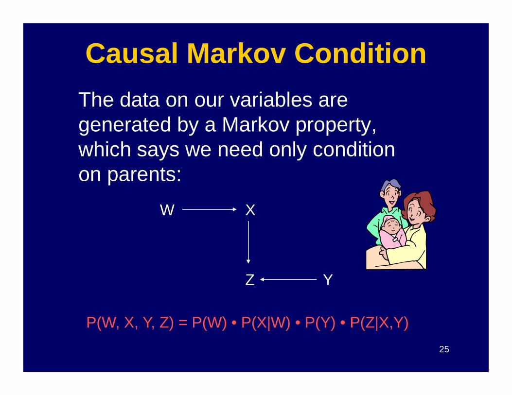
Causal Markov Condition

The data on our variables aregenerated by a Markov property,which says we need only condition on parents:

25

Z

X

Y

W

P(W, X, Y, Z) = P(W) • P(X|W) • P(Y) • P(Z|X,Y)

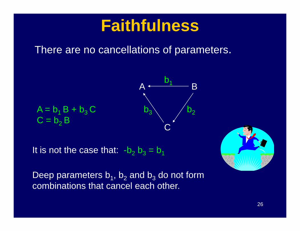
FaithfulnessThere are no cancellations of parameters.

BAb1

b2b3A = b1 B + b3 CC = b B

26

C

1 3 C = b2 B

It is not the case that: -b2 b3 = b1

Deep parameters b1, b2 and b3 do not form combinations that cancel each other.

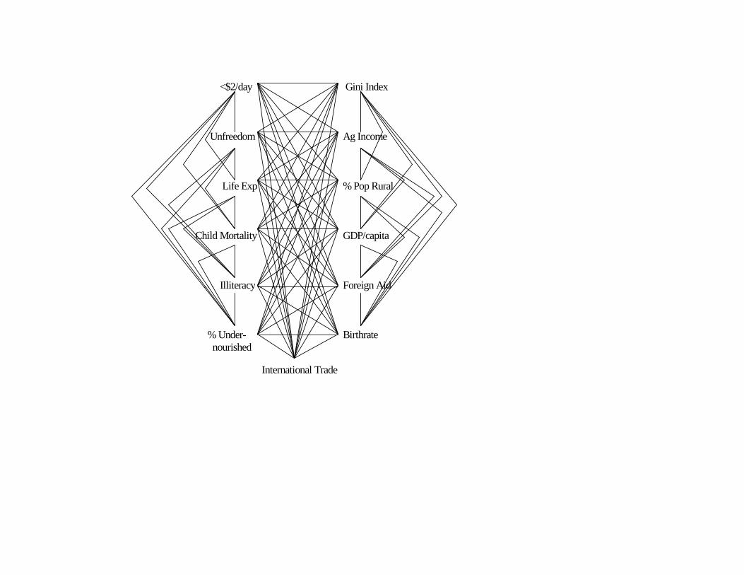
<$2/day Gini Index Unfreedom Ag Income Life Exp % Pop Rural Child Mortality GDP/capita Illiteracy Foreign Aid

27

Illiteracy Foreign Aid % Under- Birthrate nourished International Trade

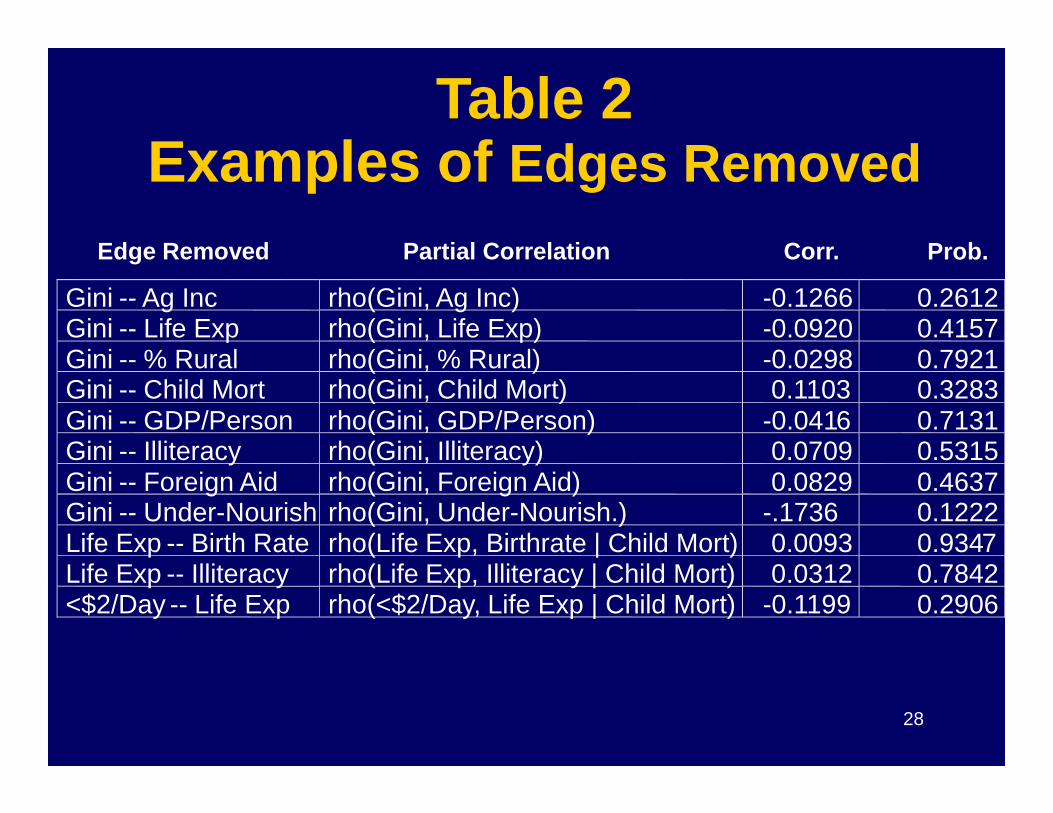
Table 2Examples of Edges Removed

Edge Removed Partial Correlation Corr. Prob.

Gini -- Ag Inc rho(Gini, Ag Inc) -0.1266 0.2612Gini -- Life Exp rho(Gini, Life Exp) -0.0920 0.4157Gini -- % Rural rho(Gini, % Rural) -0.0298 0.7921Gini -- Child Mort rho(Gini, Child Mort) 0.1103 0.3283Gini -- GDP/Person rho(Gini, GDP/Person) -0.0416 0.7131

28

Gini -- GDP/Person rho(Gini, GDP/Person) -0.0416 0.7131Gini -- Illiteracy rho(Gini, Illiteracy) 0.0709 0.5315Gini -- Foreign Aid rho(Gini, Foreign Aid) 0.0829 0.4637Gini -- Under-Nourish rho(Gini, Under-Nourish.) -.1736 0.1222Life Exp -- Birth Rate rho(Life Exp, Birthrate | Child Mort) 0.0093 0.9347Life Exp -- Illiteracy rho(Life Exp, Illiteracy | Child Mort) 0.0312 0.7842<$2/Day -- Life Exp rho(<$2/Day, Life Exp | Child Mort) -0.1199 0.2906

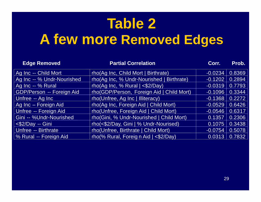
Edge Removed Partial Correlation Corr. Prob.

Table 2A few more Removed Edges

Ag Inc -- Child Mort rho(Ag Inc, Child Mort | Birthrate) -0.0234 0.8369Ag Inc -- % Undr-Nourished rho(Ag Inc, % Undr-Nourished | Birthrate) -0.1202 0.2894Ag Inc -- % Rural rho(Ag Inc, % Rural | <$2/Day) -0.0319 0.7793GDP/Person -- Foreign Aid rho(GDP/Person, Foreign Aid | Child Mort) -0.1096 0.3344Unfree -- Ag Inc rho(Unfree, Ag Inc | Illiteracy) -0.1368 0.2272

29

Unfree -- Ag Inc rho(Unfree, Ag Inc | Illiteracy) -0.1368 0.2272Ag Inc – Foreign Aid rho(Ag Inc, Foreign Aid | Child Mort) -0.0529 0.6426Unfree -- Foreign Aid rho(Unfree, Foreign Aid | Child Mort) -0.0546 0.6317Gini -- %Undr-Nourished rho(Gini, % Undr-Nourished | Child Mort) 0.1357 0.2306<$2/Day -- Gini rho(<$2/Day, Gini | % Undr-Nourised) 0.1075 0.3438Unfree -- Birthrate rho(Unfree, Birthrate | Child Mort) -0.0754 0.5078% Rural -- Foreign Aid rho(% Rural, Foreig n Aid | <$2/Day) 0.0313 0.7832

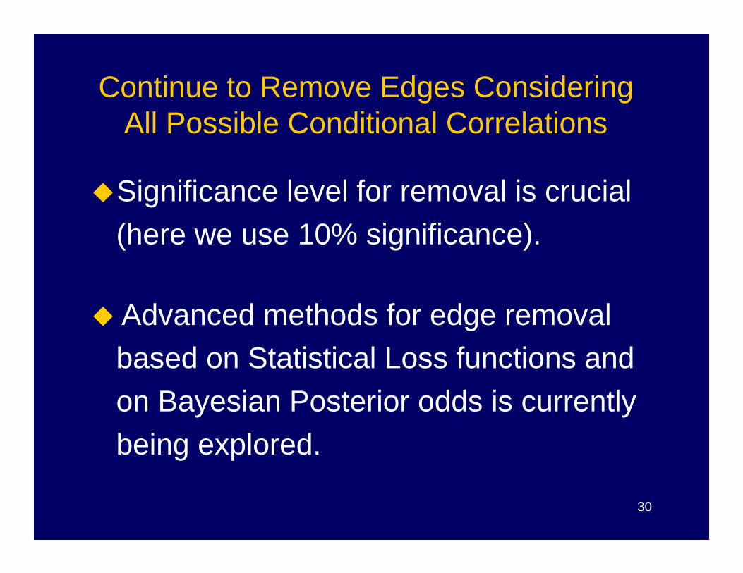
Continue to Remove Edges Considering All Possible Conditional Correlations

�Significance level for removal is crucial(here we use 10% significance).

30

� Advanced methods for edge removal based on Statistical Loss functions and on Bayesian Posterior odds is currently being explored.

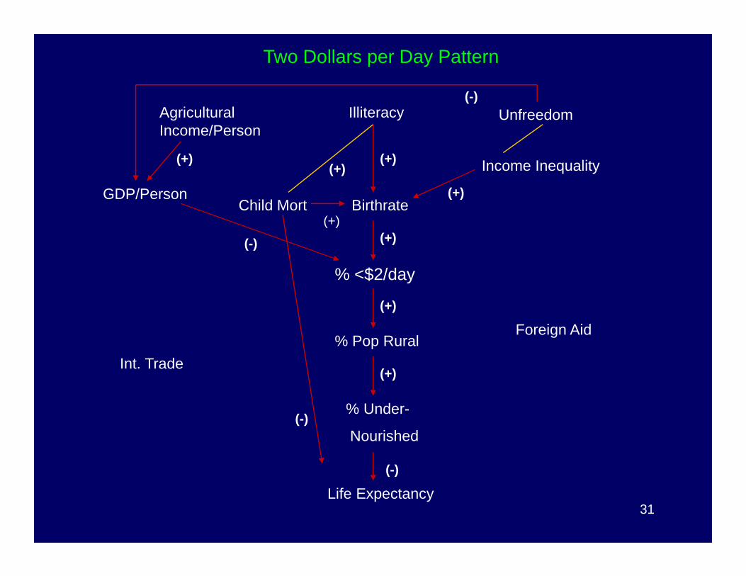
GDP/Person

Agricultural Income/Person

Illiteracy Unfreedom

Income Inequality

% <$2/day

BirthrateChild Mort(+)

(+)

(+)(+)

(+)

(-)

(-)

(+)

Two Dollars per Day Pattern

31Life Expectancy

% Under-

Nourished

% Pop RuralForeign Aid

(+)

(+)

(-)

(-)

Int. Trade

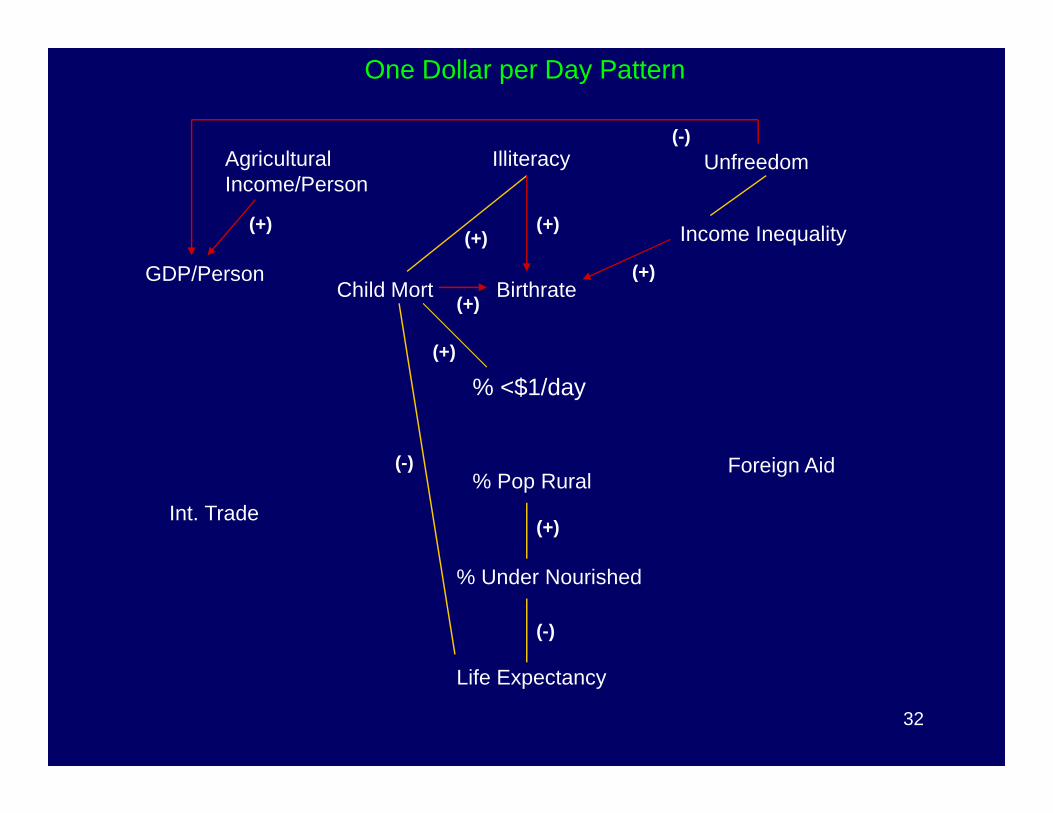
GDP/Person

Agricultural Income/Person

Illiteracy Unfreedom

Income Inequality

% <$1/day

BirthrateChild Mort(+)

(+)(+)

(+)

(-)

(+)

(+)

One Dollar per Day Pattern

32

Life Expectancy

% Under Nourished

% Pop RuralForeign Aid

(+)

(-)

Int. Trade

(-)

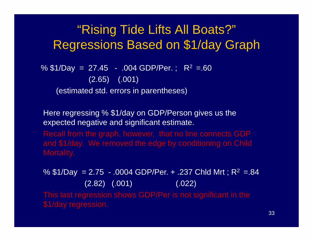
“Rising Tide Lifts All Boats?”Regressions Based on $1/day Graph

% $1/Day = 27.45 - .004 GDP/Per. ; R2 =.60(2.65) (.001)

(estimated std. errors in parentheses)

Here regressing % $1/day on GDP/Person gives us the expected negative and significant estimate.

33

expected negative and significant estimate. Recall from the graph, however, that no line connects GDP and $1/day. We removed the edge by conditioning on Child Mortality.

% $1/Day = 2.75 - .0004 GDP/Per. + .237 Chld Mrt ; R2 =.84(2.82) (.001) (.022)

This last regression shows GDP/Per is not significant in the $1/day regression.

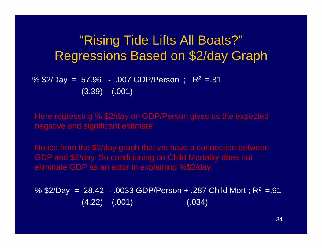
“Rising Tide Lifts All Boats?”Regressions Based on $2/day Graph

% $2/Day = 57.96 - .007 GDP/Person ; R2 =.81(3.39) (.001)

Here regressing % $2/day on GDP/Person gives us the expected negative and significant estimate!

34

negative and significant estimate!

Notice from the $2/day graph that we have a connection between GDP and $2/day. So conditioning on Child Mortality does not eliminate GDP as an actor in explaining %$2/day.

% $2/Day = 28.42 - .0033 GDP/Person + .287 Child Mort ; R2 =.91(4.22) (.001) (.034)

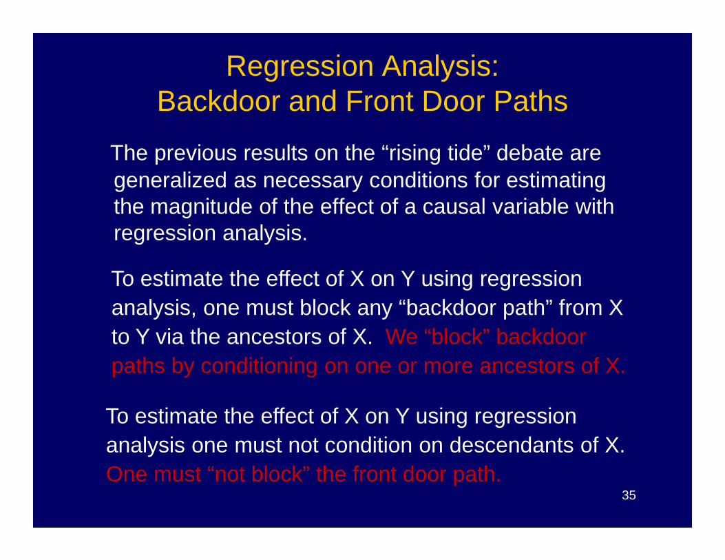
Regression Analysis: Backdoor and Front Door Paths

The previous results on the “rising tide” debate are generalized as necessary conditions for estimating the magnitude of the effect of a causal variable with regression analysis.

To estimate the effect of X on Y using regression

35

To estimate the effect of X on Y using regression analysis, one must block any “backdoor path” from X to Y via the ancestors of X. We “block” backdoor paths by conditioning on one or more ancestors of X.

To estimate the effect of X on Y using regression analysis one must not condition on descendants of X. One must “not block” the front door path.

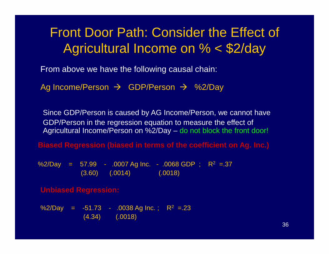
Front Door Path: Consider the Effect of Agricultural Income on % < $2/day

From above we have the following causal chain:

Ag Income/Person � GDP/Person � %2/Day

Since GDP/Person is caused by AG Income/Person, we cannot have GDP/Person in the regression equation to measure the effect of Agricultural Income/Person on %2/Day – do not block the front door!

36

Agricultural Income/Person on %2/Day – do not block the front door!

Biased Regression (biased in terms of the coefficient on Ag. Inc.)

%2/Day = 57.99 - .0007 Ag Inc. - .0068 GDP ; R2 =.37(3.60) (.0014) (.0018)

Unbiased Regression:

%2/Day = -51.73 - .0038 Ag Inc. ; R2 =.23(4.34) (.0018)

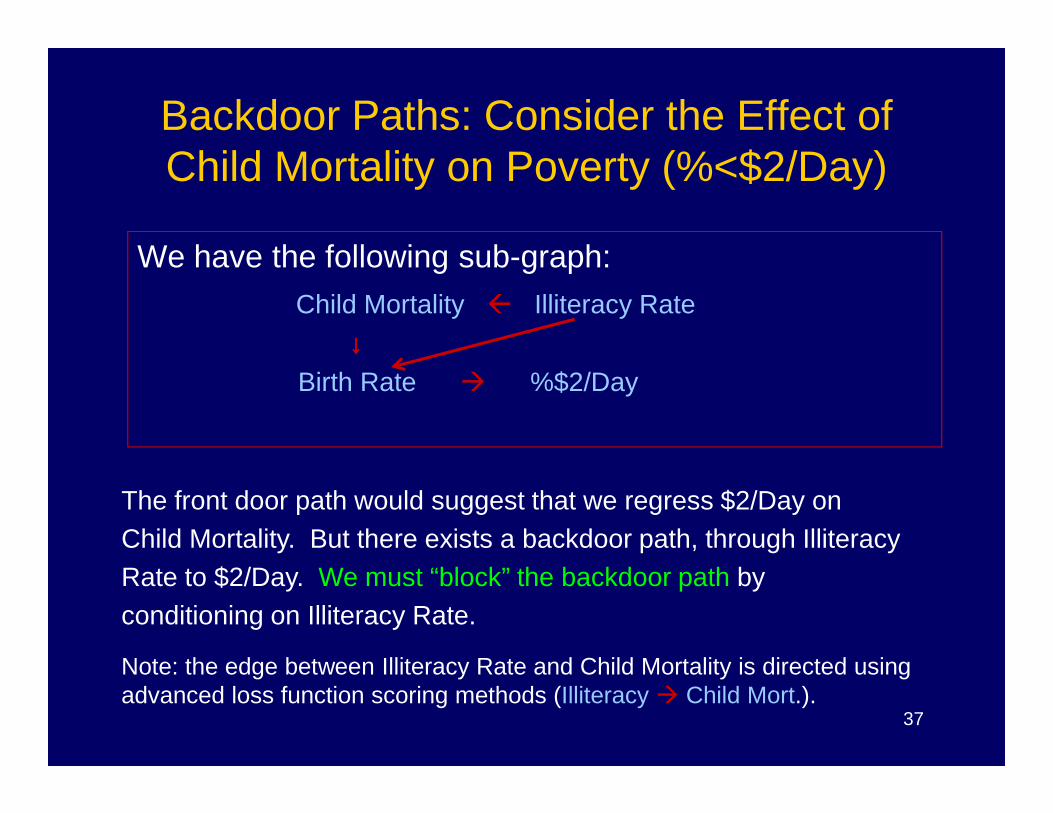
Backdoor Paths: Consider the Effect of Child Mortality on Poverty (%<$2/Day)

We have the following sub-graph:Child Mortality Illiteracy Rate

↓↓↓↓Birth Rate � %$2/Day

37

The front door path would suggest that we regress $2/Day onChild Mortality. But there exists a backdoor path, through IlliteracyRate to $2/Day. We must “block” the backdoor path by conditioning on Illiteracy Rate.

Note: the edge between Illiteracy Rate and Child Mortality is directed using advanced loss function scoring methods (Illiteracy � Child Mort.).

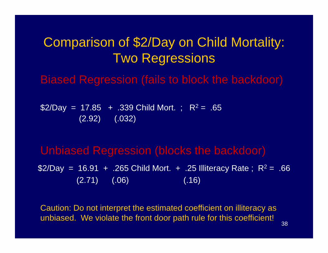
Comparison of $2/Day on Child Mortality: Two Regressions

Biased Regression (fails to block the backdoor)

$2/Day = 17.85 + .339 Child Mort. ; R2 = .65(2.92) (.032)

38

Unbiased Regression (blocks the backdoor)$2/Day = 16.91 + .265 Child Mort. + .25 Illiteracy Rate ; R2 = .66

(2.71) (.06) (.16)

Caution: Do not interpret the estimated coefficient on illiteracy as unbiased. We violate the front door path rule for this coefficient!

ConclusionsGiven our set of variables: Illiteracy, Freedom, and Agricultural Income are exogenous movers of (root causes of) poverty.

Given the assumptions in the directed graphs literature, we can consider manipulations of poverty by manipulations in one or more of these causes.

39

one or more of these causes.

Use of regression techniques to measure the quantitative relationship between causes and effects requires that we block backdoor paths and not block front door paths.

Whether or not any of these can be “easily” manipulated is, of course, another question.

Caution

Our methods assume:

� Causal Sufficiency

� Markov Property

� Faithfulness

40

� Faithfulness

� Normality

Failure of any of these may change results.

More Caution: Duhem’s Thesis

Foreign Aid may be better measured (for ourpurposes) as Foreign Aid for Poverty Alleviation(the variable we use is Total Foreign Aid).

41

International trade might well be measured withoutnatural resource exports (Dutch Disease).

Dynamic representation of poverty should be pursued. This will require a richer data set.

Acknowledgements

Motivation for the study

Aysen Tanyeri-Abur, FAO

42

Motivation for our study of Directed Graphs

Clark Glymour, CMU

Judea Pearl, UCLA

Comments from Granger

• June 3 2003

• Dear David,

• Thanks for your slides about causality and DAGS. I certainly think that • poverty is a very important topic and well worth studying. DAGS can • sometimes be helpful in suggesting causality, but are not without • problems. It is useful to require a time passage between cause and effect • but this is not always clear in DAGS. I can only partly agree with your • central point on page 11; a theory is helpful only if it is correct (a bad

43

• central point on page 11; a theory is helpful only if it is correct (a bad • theory can be misleading) but how can you tell if the theory is correct?

• I think that poverty data will always be non-experimental. Your statement • on slide 15 is quite controversial although some writers equate causality • and controlability (Hoover does), most do not (Pearl seems to be unclear in • discussions). I think that control is a much deeper question and needs a • separate definition.

• I hope these comments are helpful.

• Yours sincerely,

• Clive W.J. Granger• Professor of Economics