Embed Size (px)
Citation preview

Direct-Write Digital Holography
Development and research of a hologram printer
John Peter Tapsell
Submitted for the degree of Doctor of Philosophy
University of Sussex
April 2008

To my wife, Saki.

Declaration
I hereby declare that this thesis, either in the same or different form, has not been
previously submitted to this or any other University for a degree.
Signature:
John Peter Tapsell
iii
UNIVERSITY OF SUSSEX
JOHN PETER TAPSELL, DOCTOR OF PHILOSOPHY
DIRECT-WRITE DIGITAL HOLOGRAPHY
DEVELOPMENT AND RESEARCH OF A HOLOGRAM PRINTER
SUMMARY
Chapter 1 gives a brief history of the field of holography along with an overview
of this thesis. A more detailed description of holography is provided in Chapter 2
along with a discussion of digital holography. Chapter 3 examines the design of a
one-step monochromatic hologram printer capable producing white-light view-
able transmission holograms created with the aid of an LCOS display system and
printed in a dot-matrix sequence. The lens system employed includes a microlens
array and an afocal relay telescope which are both quantitatively examined in or-
der to maximise the contrast, diffraction efficiency and depth of view of the final
hologram image. A brief overview of speckle reduction techniques and their ap-
plicability to pulsed digital holography is presented along with experimental re-
sults of the use of a microlens array to reduce speckle effects. Chapter 4 presents
an analysis of the unwanted side effects of the angular intensity distribution of a
hologram pixel, using a case study for analysis. Chapter 5 examines methods for
increasing both the printing speed and resolution of the hologram printer. Chap-
ter 6 describes the analysis and design of a temperature-energy feedback system
to correct for pulsed laser instabilities arising from mode beating due to tem-
perature variations. Chapter 7 provides a conclusion to the work and discusses
possible future developments.
iv

Acknowledgements
I would first like to thank the people who made this project possible: My uni-
versity supervisors Professor Chris Chatwin and Dr. Rupert Young for their help
and encouragement; and my work supervisor Dr. David Brotherton-Ratcliffe and
the staff at Geola Technologies for allowing me to break much of their valuable
equipment over the three years of employment. I would also like to make a spe-
cial mention to Doug Ollivier for his permission for the use of his 3D futuristic-
tank model.
A special thanks goes out to my brother, Ian Kevin Tapsell, who spent many
days and nights working with me in the dark room handling the chemicals and
processing the holograms with expert ease.
I would also like to acknowledge the support of a EPSRC fellowship. This
work was funded by the UK’s leading funding agency - the Engineering and
Physical Sciences Research Council. Without this opportunity, I never would
have delved into the world of physics and engineering.
Finally, my warmest appreciation goes to my darling wife Saki Tapsell, who
looked after me at every step of the way. Without her, none of this would have
been possible.
v

CONTENTS
Contents
Contents ix
1 Introduction 1
1.1 Holography . . . . . . . . . . . . . . . . . . . . . . . . . . . . . . . . 1
1.2 Overview of thesis . . . . . . . . . . . . . . . . . . . . . . . . . . . . 3
2 Background 4
2.1 Definition . . . . . . . . . . . . . . . . . . . . . . . . . . . . . . . . . 4
2.2 A brief introduction to photography . . . . . . . . . . . . . . . . . . 5
2.3 History of holography . . . . . . . . . . . . . . . . . . . . . . . . . . 6
2.4 Digital versus analogue . . . . . . . . . . . . . . . . . . . . . . . . . 17
3 Design of a digital hologram printer 19
3.1 Overview . . . . . . . . . . . . . . . . . . . . . . . . . . . . . . . . . . 19
3.2 Detail of system components . . . . . . . . . . . . . . . . . . . . . . 23
3.2.1 Laser system . . . . . . . . . . . . . . . . . . . . . . . . . . . 24
3.2.2 Optics for transport of beams . . . . . . . . . . . . . . . . . . 25
3.2.3 Digital display system . . . . . . . . . . . . . . . . . . . . . . 26
3.3 Analysis of lens system . . . . . . . . . . . . . . . . . . . . . . . . . . 30
3.3.1 Lenses L1 and L2 . . . . . . . . . . . . . . . . . . . . . . . . . 38
3.3.2 Lenses L3 and L4 . . . . . . . . . . . . . . . . . . . . . . . . . 38
vi
CONTENTS
3.3.3 Lenses L2 and L3 . . . . . . . . . . . . . . . . . . . . . . . . . 39
3.3.4 Focal length approximations . . . . . . . . . . . . . . . . . . 40
3.3.5 Optical system for microlens array . . . . . . . . . . . . . . . 40
3.3.6 Summary . . . . . . . . . . . . . . . . . . . . . . . . . . . . . 47
3.3.7 Example microlens array . . . . . . . . . . . . . . . . . . . . 48
3.4 Experimental evaluation of lens array system . . . . . . . . . . . . . 51
3.4.1 Previous work . . . . . . . . . . . . . . . . . . . . . . . . . . . 52
3.4.2 Experimental setup . . . . . . . . . . . . . . . . . . . . . . . . 54
3.4.3 Image quality . . . . . . . . . . . . . . . . . . . . . . . . . . . 55
3.4.4 Speckle repeating structure size . . . . . . . . . . . . . . . . . 59
3.4.5 Microlens array focal plane . . . . . . . . . . . . . . . . . . . 61
3.4.6 Summary . . . . . . . . . . . . . . . . . . . . . . . . . . . . . 63
3.5 Minimizing beam energy loss in lens system . . . . . . . . . . . . . 65
3.6 Summary . . . . . . . . . . . . . . . . . . . . . . . . . . . . . . . . . . 67
4 White logo 69
4.1 Overview . . . . . . . . . . . . . . . . . . . . . . . . . . . . . . . . . . 69
4.2 Photograph analysis . . . . . . . . . . . . . . . . . . . . . . . . . . . 73
4.3 Spectrometer . . . . . . . . . . . . . . . . . . . . . . . . . . . . . . . . 80
4.4 Future work . . . . . . . . . . . . . . . . . . . . . . . . . . . . . . . . 85
4.5 Summary . . . . . . . . . . . . . . . . . . . . . . . . . . . . . . . . . . 88
5 Printing speed and resolution improvements 89
5.1 Overview . . . . . . . . . . . . . . . . . . . . . . . . . . . . . . . . . . 89
5.2 Power supply . . . . . . . . . . . . . . . . . . . . . . . . . . . . . . . 90
5.3 Stability . . . . . . . . . . . . . . . . . . . . . . . . . . . . . . . . . . . 91
5.4 Software . . . . . . . . . . . . . . . . . . . . . . . . . . . . . . . . . . 96
5.5 Display system refresh rates . . . . . . . . . . . . . . . . . . . . . . . 98
5.6 Stage movement . . . . . . . . . . . . . . . . . . . . . . . . . . . . . . 99
5.7 Increasing printed holopixel resolution . . . . . . . . . . . . . . . . 100
vii
CONTENTS
5.8 3D model . . . . . . . . . . . . . . . . . . . . . . . . . . . . . . . . . . 103
5.9 Analysis . . . . . . . . . . . . . . . . . . . . . . . . . . . . . . . . . . 109
5.10 Summary . . . . . . . . . . . . . . . . . . . . . . . . . . . . . . . . . . 112
6 Temperature-energy feedback 113
6.1 Problems with laser instability . . . . . . . . . . . . . . . . . . . . . 113
6.2 Custom energy meter . . . . . . . . . . . . . . . . . . . . . . . . . . . 116
6.2.1 Overview of custom energy meter . . . . . . . . . . . . . . . 117
6.2.2 Methods for diverting beam . . . . . . . . . . . . . . . . . . . 117
6.2.3 Calibrating custom energy meter . . . . . . . . . . . . . . . . 119
6.3 Digital temperature controller . . . . . . . . . . . . . . . . . . . . . . 124
6.4 Temperature feedback algorithm . . . . . . . . . . . . . . . . . . . . 125
6.5 Temperature feedback system on rear mirror . . . . . . . . . . . . . 127
6.6 DTC-PC communication . . . . . . . . . . . . . . . . . . . . . . . . . 129
6.7 Temperature-energy feedback . . . . . . . . . . . . . . . . . . . . . . 131
6.8 Summary . . . . . . . . . . . . . . . . . . . . . . . . . . . . . . . . . . 135
7 Conclusion and future work 136
7.1 Conclusion . . . . . . . . . . . . . . . . . . . . . . . . . . . . . . . . . 136
7.2 Future work . . . . . . . . . . . . . . . . . . . . . . . . . . . . . . . . 140
A Program listing for image cropping 150
B DTC commands 151
C Hologram printer diagrams 153
D Program listing for image analysis 160
E Optical fourier transform lens system 162
F LCOS mechanical mount 166
G Lens system 168
viii
CONTENTS
H Laser specifications 170
I Microlens array analysis 173
I.1 First microlens array . . . . . . . . . . . . . . . . . . . . . . . . . . . 175
I.2 Second microlens array . . . . . . . . . . . . . . . . . . . . . . . . . . 178
I.3 Third microlens array . . . . . . . . . . . . . . . . . . . . . . . . . . . 180
J Hologram printer photographs 182
ix

LIST OF TABLES
List of Tables
3.1 Microlens array properties . . . . . . . . . . . . . . . . . . . . . . . . 49
3.2 Size of repeating speckle structure . . . . . . . . . . . . . . . . . . . 59
3.3 Distance between microlens array focal plane and aperture . . . . . 62
4.1 Technical details of spectrometer . . . . . . . . . . . . . . . . . . . . 82
4.2 Spectrometer results . . . . . . . . . . . . . . . . . . . . . . . . . . . 83
4.3 Photograph intensity for spectrometer results . . . . . . . . . . . . . 83
5.1 Maximum reference and object beam separation distance . . . . . . 94
5.2 Maximum angle deviation for a photographic plate . . . . . . . . . 102
B.1 Communication protocol for Digital Temperature Controller . . . . 152
G.1 Lens system optical components . . . . . . . . . . . . . . . . . . . . 169
H.1 Specifications of laser used . . . . . . . . . . . . . . . . . . . . . . . . 172
I.1 Raw data results for first lens array . . . . . . . . . . . . . . . . . . . 177
I.2 Raw data results for second lens array . . . . . . . . . . . . . . . . . 179
I.3 Raw data results for third lens array . . . . . . . . . . . . . . . . . . 181
x

LIST OF FIGURES
List of Figures
2.1 First permanent photograph, by Niépce in 1826 . . . . . . . . . . . . 5
2.2 Wire diffraction grating, similar to that made by Fraunhofer . . . . 8
2.3 Dennis Gabor . . . . . . . . . . . . . . . . . . . . . . . . . . . . . . . 8
2.4 Yuri Denisyuk . . . . . . . . . . . . . . . . . . . . . . . . . . . . . . . 10
2.5 Theodore H. Maiman . . . . . . . . . . . . . . . . . . . . . . . . . . . 11
3.1 Hologram printer by Ratcliffe et al. . . . . . . . . . . . . . . . . . . . 22
3.2 Hologram Printer with LCOS . . . . . . . . . . . . . . . . . . . . . . 23
3.3 Top-down orthographic projection of Hologram Printer with LCOS 24
3.4 Length adjustment system . . . . . . . . . . . . . . . . . . . . . . . . 25
3.5 Lens system . . . . . . . . . . . . . . . . . . . . . . . . . . . . . . . . 28
3.6 Photograph of LCOS being illuminated . . . . . . . . . . . . . . . . 29
3.7 Object lens system on printer . . . . . . . . . . . . . . . . . . . . . . 31
3.8 Ray-traced lens setup 1 . . . . . . . . . . . . . . . . . . . . . . . . . . 33
3.9 Ray-traced lens setup 2 . . . . . . . . . . . . . . . . . . . . . . . . . . 33
3.10 Logical diagram of optical beam path layout . . . . . . . . . . . . . 37
3.11 Effective focal length of lens L4 . . . . . . . . . . . . . . . . . . . . . 41
3.12 Brillian LCOS Display BR1080HC . . . . . . . . . . . . . . . . . . . . 49
3.13 Quality of the projected image due to speckle . . . . . . . . . . . . . 56
3.14 Suitable positions for first microlens array . . . . . . . . . . . . . . . 57
3.15 Suitable positions for second microlens array . . . . . . . . . . . . . 58
xi

LIST OF FIGURES
3.16 Suitable positions for third microlens array . . . . . . . . . . . . . . 58
3.17 Speckle structure against microlens array array position . . . . . . . 60
3.18 Distance between microlens array focal plane and aperture images 63
3.19 Photograph of dragon hologram . . . . . . . . . . . . . . . . . . . . 68
4.1 Viewing-window comparison . . . . . . . . . . . . . . . . . . . . . . 71
4.2 White Logo photograph and rendered images . . . . . . . . . . . . 74
4.3 Photograph intensity against rendered image intensity . . . . . . . 75
4.4 Photograph minus image intensity against total image intensity . . 77
4.5 Corrected image . . . . . . . . . . . . . . . . . . . . . . . . . . . . . . 77
4.6 Corrected image with each channel corrected separately . . . . . . 78
4.7 Photograph minus image against total (Individual channels) . . . . 79
4.8 Photograph of framework for spectrometer and halogen light . . . 80
4.9 Photograph of fine-control spectrometer mount . . . . . . . . . . . . 81
4.10 Photograph of spectrometer in use . . . . . . . . . . . . . . . . . . . 82
4.11 Spectrometer readings against photograph readings . . . . . . . . . 84
4.12 Photograph of hologram with decreasing viewing window . . . . . 86
4.13 Photograph of hologram with decreasing viewing window and en-
ergy . . . . . . . . . . . . . . . . . . . . . . . . . . . . . . . . . . . . . 87
5.1 Diagram of intersection plane of hologram plate and beams . . . . 92
5.2 Object and reference beam misalignment . . . . . . . . . . . . . . . 93
5.3 Behavior of Microsoft Windows sleep() function . . . . . . . . . 97
5.4 Rendered model images . . . . . . . . . . . . . . . . . . . . . . . . . 105
5.5 Large rendered model image . . . . . . . . . . . . . . . . . . . . . . 106
5.6 High resolution hologram of a futuristic tank . . . . . . . . . . . . . 110
5.7 Zoomed in on a small section of the high resolution hologram . . . 111
6.1 Diffraction efficiency curve for VRP-M emulsion . . . . . . . . . . . 115
6.2 Two possible layouts to deflect energy to the detector . . . . . . . . 118
6.3 Comparison of energy readings for mirror-leakage method . . . . . 119
xii

LIST OF FIGURES
6.4 Measured voltage on custom energy meter . . . . . . . . . . . . . . 120
6.5 Theoretical voltage on custom energy meter . . . . . . . . . . . . . . 122
6.6 Comparison of custom energy meter vs. Ophir’s . . . . . . . . . . . 123
6.7 Photograph of DTC . . . . . . . . . . . . . . . . . . . . . . . . . . . . 124
6.8 DTC response to target temperature changes . . . . . . . . . . . . . 128
6.9 DTC response to noise in temperature readings . . . . . . . . . . . . 128
6.10 Breadboard temperature against time . . . . . . . . . . . . . . . . . 129
6.11 Energy against time in rear mirror position scan over 20 hours . . . 131
6.12 Energy temperature feedback algorithm . . . . . . . . . . . . . . . . 133
6.13 Pulse energy with active feedback . . . . . . . . . . . . . . . . . . . 134
6.14 Pulse std. dev. with active feedback . . . . . . . . . . . . . . . . . . 134
7.1 Photograph of dragon hologram . . . . . . . . . . . . . . . . . . . . 139
7.2 High resolution hologram of a futuristic tank . . . . . . . . . . . . . 139
A.1 Program for cropping images with a sliding window . . . . . . . . 150
C.1 Original hologram printer with LCD . . . . . . . . . . . . . . . . . . 154
C.2 Hologram printer with LCOS . . . . . . . . . . . . . . . . . . . . . . 155
C.3 Layout of Hologram Printer . . . . . . . . . . . . . . . . . . . . . . . 156
C.4 Layout of Hologram Printer with dimensions . . . . . . . . . . . . . 157
C.5 Length adjustment system . . . . . . . . . . . . . . . . . . . . . . . . 158
C.6 Object lens system on printer . . . . . . . . . . . . . . . . . . . . . . 159
D.1 Program for White Logo analysis . . . . . . . . . . . . . . . . . . . . 161
E.1 Lens system for imaging LCOS Fourier image . . . . . . . . . . . . 163
E.2 Compound Lens L2 . . . . . . . . . . . . . . . . . . . . . . . . . . . . 163
E.3 Compound Lens L3 . . . . . . . . . . . . . . . . . . . . . . . . . . . . 164
E.4 Compound Lens L4 . . . . . . . . . . . . . . . . . . . . . . . . . . . . 164
E.5 Objective Lens system, ray traced . . . . . . . . . . . . . . . . . . . . 165
xiii

LIST OF FIGURES
F.1 Side-on orthogonal view of mechanical mount for LCOS and split
beam polariser . . . . . . . . . . . . . . . . . . . . . . . . . . . . . . . 167
H.1 Photograph of laser, powersupply and cooling unit . . . . . . . . . 171
H.2 Photograph of laser case . . . . . . . . . . . . . . . . . . . . . . . . . 171
J.1 Photograph of part of the hologram printer . . . . . . . . . . . . . . 183
J.2 Photograph of me working on the hologram printer . . . . . . . . . 184
J.3 Photograph of LCOS section of the hologram printer . . . . . . . . 185
J.4 Photograph of short cavity laser . . . . . . . . . . . . . . . . . . . . . 186
xiv

LIST OF ALGORITHMS
List of Algorithms
1 Printing algorithm suitable for printing at low speed . . . . . . . . . 96
2 DTC feedback using PID algorithm . . . . . . . . . . . . . . . . . . . 126
xv

LIST OF ACRONYMS
List of Acronyms
SLM Spacial Light Modulator. A device that spatially modulates a beam of light.
EASLM Electrically Addressed Spacial Light Modulator. A SLM display that is
electrically (as opposed to optically) controlled, typically by a computer.
LCD Liquid Crystal Display. In this usage, a transmissive EASLM display that
spatially modulates the beam intensity.
LCOS Liquid Crystal On Silicon. A reflective EASLM display that spatially mod-
ulates the beam phase. Used in conjunction with a polariser to modulate the
intensity.
Nd:YAG Neodymium Doped Yttrium Aluminum Garnet. A lasing material used
in near-infrared lasers.
VSYNC Vertical Synchronization. Matching a display (such as an SLM) refresh
rate.
CW Continuous Wave. A laser beam that is continuous, rather than pulsed.
3D Three-Dimensional. A three dimensional object or image.
2D Two-Dimensional. A two dimensional image, without depth. Such as a pho-
tograph.
xvi
LIST OF ACRONYMS
2.5D 2.5 Dimensional. An image with, typically, horizontal but not vertical par-
allax.
CCD Charge-coupled device. A device that enables electric charges to be trans-
ported through successive capacitors controlled by a clock signal. Used
mainly for sensors that capture and record light.
DTC Digital Temperature Controller. The name we gave to the PCB that heats
and measures the temperature of a component.
PCB Printed Circuit Board. A board for supporting, mounting and connecting
electronic components.
PID Proportional Integral Derivative. A standard algorithm to change an output
in response to an input.
ID identification number. Assigned unique number for identification.
USB Universal Serial Bus. A serial bus standard for communication between
devices.
PC Personal Computer.
A-D Analogue-Digital.
EIA Electronics Industry Alliance. A trade organization for electronics manufac-
turers in the United States.
DPI Dots Per Inch. The number of dots (pixels) per linear inch.
RGB Red Green Blue. Three additive primary colors.
I/O Input/Output. Input and output data streams.
OS Operating System. The software that manages the computer’s hardware re-
sources.
xvii

LIST OF ACRONYMS
NDF Neutral Density Filter. A darkened piece of glass used to decrease the en-
ergy of a laser beam.
xviii

NOMENCLATURE
(Page numbers indicate the first use of the variable)
Hologram printer components
The components in the hologram printer are labelled uniquely throughout the
thesis. See Appendix C for full page schematic labelled diagrams.
L1 Lens between microlens array and LCOS.
L2 First compound lens in relay telescope to image LCOS to plane I2
L3 Second compound lens in relay telescope to image LCOS to plane I2
L4 Objective compound lens, to image the Fourier plane of I2 onto I3
L5 First lens in afocal telescope in object beam to magnify the beam
L6 Second lens in afocal telescope in object beam to magnify the beam
L7 Acts with lens L8 to image I4 to I3
L8 Acts with lens L7 to image I4 to I3
L9 Acts with lens L10 to image aperture to image I4
L10 Acts with lens L9 to image aperture to image I4
LCOS LCOS display system
I1 Real focal image plane inside relay telescope
I2 Real focal image plane inside relay telescope
I3 Real holopixel plane. Fourier transform of LCOS
I4 Real image plane of aperture
I5 Focal plane of L10 and L9 - aperture placed here to clean beam
A Microlens array
a Optical distance from microlens array to lens L1
b Optical distance from lens L1 to LCOS, via mirror and cube polariser
c Optical distance from LCOS to lens L2 via split beam polariser
d Optical distance from lens L2 to image plane I1
e Optical distance from image plane I1 to lens L3
f Optical distance from lens L3 to image plane I2
xix

NOMENCLATURE
g Optical distance from image plane I2 to lens L4
h Optical distance from lens L4 to image plane I3
j Optical distance from image plane I3 to lens L7
k Optical distance from between lenses L7 and L8
m Optical distance from lens L8 to image plane I4
n Optical distance from image plane I4 to lens L9
y Width of aperture on microlens array A
z Distance between aperture and microlens array
Laser Laser mounted on breadboard
Equation reference
Sensitivity analysis
Provides a measure of the sensitivity of a function with respect to one of its input
variables. A value of << 1 means the output of the function is very insensitive to
changes in the variable. A value of >> 1 means that the output of the function is
very sensitive to changes in the variable.
Relative sensitivity of f w.r.t. x =x
f· ∂f∂x
(1)
Lens equations
The thin lens formula in air is:
1
S1
+1
S2
=1
f(2)
Where S1 is the distance between an object plane and a thin lens with focal length
f and S2 is the distance between the thin lens and the image plane.
xx

NOMENCLATURE
For two thin lenses with focal lengths f1 and f2 respectively, separated by an
optical distance of f1+f2 , the final convergence of the beam is not altered (making
it afocal), but the width of the beam is magnified by a factor M of:
M = −f1
f2
(3)
Small angle approximation for paraxial rays:
sin(θ) ≈ θ (4)
Matrix method for lens system analysis
The matrix method for lens system analysis works on the basis that a thin-lens
system can be described with a matrix, M . The input vector, vinput, is modified
by the matrix to produce the output vector, vfinal as so:
vfinal = M · vinput (5)
Vector for light ray at height r and travelling at angle θ from the horizontal (From
Chartier [1, pages 120-130]):
v = (r, θ)T (6)
Transfer matrix for ray travelling distance b in constant medium:
M =
1 b
0 1
(7)
xxi

NOMENCLATURE
Lens matrix for ray travelling through a thin-lens with focus f :
M =
1 0
− 1
f1
(8)
Matrix for surface with initial index of refraction n1, final index of refraction n2
and curvature R:
M =
1 0
n1−n2
R·n2
n1
n2
(9)
xxii

1Introduction
1.1 Holography
To watch a person’s first interaction with a hologram is a truly fascinating ex-
perience. They cannot help but try to reach out and touch the object that they
can see projected out in front of them, but know is not really there. A large full
colour hologram can be a beautiful, albeit expensive, piece of artwork, projecting
a Three-Dimensional (3D) holographic image producing all of the visual impres-
sions of depth and realism that is found in real scenes. Holography has tradition-
ally required a real object from which to make the hologram, but recent advances
in digital holography have allowed the production of realistic holographic im-
ages of scenes and objects that exist only in the mind of the artist. Digital holog-
raphy is already being used in numerous applications - from artwork, to product
advertising, to data visualization.
Holography is the technique of recording 3D images by recording and replay-
1

1.1. HOLOGRAPHY
ing optical wavefronts. Gabor et al. [2] developed the mathematical toolkit for
holography just under 50 years ago. It took a further 20 years for technology to
advance sufficiently to allow researchers to reliably produce 3D holograms using
a laser[3]. Optical holographic imaging is the traditional technique of first illumi-
nating a firm rigid object with a coherent laser source. The scattered light from
the object falls upon a coated plate, interfering with a second mutually-coherent
beam. The resultant microscopic interference pattern is recorded by the high res-
olution light sensitive emulsion on the plate[3, 4]. After chemical development,
the plate can be viewed to reveal a 3D image of the original object, on a 1:1 scale.
With the goal of producing holograms that were not 1:1 scale images of real
objects, researchers looked at using Liquid Crystal Display (LCD) displays as
a replacement of the real object. Although these produce an inherently Two-
Dimensional (2D) image, by printing millions of different 2D images in a dot-
matrix style with a suitable image transformation, a 3D or 2.5 Dimensional (2.5D)
hologram image can be composed.
This thesis investigates possible improvements to an existing digital mono-
chrome holographic printer. The architecture of a digitally-based holographic
printer is directed by three main goals: (1) To produce holograms of models cre-
ated on a computer by an artist with no special knowledge of holography, (2) to
have as high a resolution, contrast and fidelity as possible, and (3) to produce
said holograms at a commercially viable rate and cost.
2

1.2. OVERVIEW OF THESIS
1.2 Overview of thesis
The following original research is documented in this thesis dissertation:
• A description of a digital hologram printer, intended to aid with the pro-
duction of a practical hologram printer.
• An analytical examination of the two main components of the lens system,
allowing for the final pixel size and shape to be predicted accurately, and
thus predicting the energy density on the holographic film. The problem
of speckle is also addressed and qualitatively assessed. This knowledge
becomes crucial for increasing the resolution, and thus decreasing the pixel
size.
• Mechanical and software improvements to a holographic printer design
based upon a sensitivity analysis, qualitative experience, and quantitative
research.
• The architecture and implementation of a temperature-energy feedback sys-
tem designed to improve stability of the pulsed laser, a key component in
the holographic printer.
• A case study analysis of the unwanted side effects of the angular intensity
distribution of a hologram pixel on its apparent intensity.
• Demonstration of improvements to produce a high resolution hologram,
recorded at 532 nm.
• Demonstration of the feasibility of using a high contrast reflective Liquid
Crystal On Silicon (LCOS) display system over the older lower contrast
transmissive LCD display system.
The following Background chapter provides a brief historical overview of
holography, focussing on the path that led to digital holography, as well as a
more detailed look at recent research in the field of digital holographic printers.
3

2Background
2.1 Definition
What is a hologram? The term hologram has been used (often incorrectly) to
mean many things – encompassing everything from a projected 3D image float-
ing in the air, to lenticular posters, to sparkly Christmas wrapping paper.
The Merriam-Webster dictionary defines it as:
‘A three-dimensional image reproduced from a pattern of interference
produced by a split coherent beam of radiation (as a laser); ’
For the purposes of this thesis, a hologram is defined to mean that the viewer
can see an apparently Three-Dimensional virtual image with at least horizontal
parallax when looking at a hologram device with the image being produced from
a pattern of interference.
For a better understanding of how a hologram works, a brief look at the his-
4

2.2. A BRIEF INTRODUCTION TO PHOTOGRAPHY
tory and theory of traditional photography is required.
2.2 A brief introduction to photography
A traditional photograph is created when ordinary white light is captured by a
light sensitive emulsion attached to some substrate. A camera captures light that
is emitted or reflected from the target objects and is focused by a series of lenses
to create a real image on the emulsion. The emulsion is made of a light sensitive
mixture (typically involving silver or chalk) that undergoes a chemical reaction
whose reaction rate has some approximately linear correlation to the intensity of
the light incident upon it. The film can then undergo wet chemical processing to
make a permanent image.
In this way, the film captures the intensity of the light. Phase information
about the light is discarded, requiring that a particular point in the scene is set
permanently as the focus point.
1724. J.H. Schultz discovered that some silver salts, for example silver chlo-
ride and silver nitrate, darken when exposed to light.
Figure 2.1: First permanent photograph, by Niépce in 1826 (Public domain)
5

2.3. HISTORY OF HOLOGRAPHY
1826. It took over a hundred years before Joseph Nicéphore Niépce used the
silver salts to make a permanent photograph based on these principles (See Fig-
ure 2.1 on the preceding page). It took 8 hours to expose this photograph.
1840. Talbot [5] developed a process to create a negative image first, creating
the today-common nomenclature ‘photograph’, ‘negative’ and ‘positive’.
1851. Archer [6] discovered1 by using a process he coined the Wet Plate Col-
lodion process the exposure time could be drastically reduced.
1884. Eastman et al. [7] invented the photographic film, replacing the photo-
graphic plate.
1975. Analogue photography does not change fundamentally until modern
digital photography is invented. Dillon et al. [8] uses solid-state Charge-coupled
device (CCD) image sensor chips to capture an image.
1990. The first true commercial digital camera is released – the Dycam Model
1; using an improved CCD image sensor.
2.3 History of holography
This section looks at development of the field of holography. Holograms in many
different forms have been developed in the second half of the 20th century. The
basic idea idea has always been the same – to create a diffraction grating on some
material in a way that ultimately ends up with a viewable picture.
Arguably a hologram is synonymous with a diffraction grating – at the techni-
cal level they are the same thing. But the distinction is analogous to the difference
between a painting and a piece of paper with paint on it. The latter is technically
the same as the painting, but may contain no picture or image that can be inter-
preted by a human eye.
1For historical accuracy, I feel obliged to note that the Collodion process was first suggestedby Mr. Le Gray[6] but published by Archer first.
6
2.3. HISTORY OF HOLOGRAPHY
Because of the technical similarity between a hologram and a diffraction grat-
ing, the advances of each tend to go hand-in-hand. So to give an explanation of
holography, a brief description of a diffraction grating is in order.
A diffraction grating is a surface covered by a pattern of parallel lines, with
the distance between the lines ideally of the order of the wavelength of visible
light. Light incident on the diffraction grating is bent or reflected due to diffrac-
tion, or absorbed. The light acts as a wave, to produce a image or a pattern. Most
literature considers diffraction gratings with a series of regularly space lines, pro-
ducing just a change in angle of the light. However throughout this thesis the
term diffraction grating will refer to a more general grating with an arbitrary-
spaced series of lines.
A brief history of the diffraction grating:
Approx 1660. James Gregory noticed that bird feathers produced diffraction
patterns, creating iridescent colors. Reflection diffraction gratings appear quite
commonly in nature, from butterfly wings, to peacock feathers and even many
beetles. Birds, for example, grow their feathers in such a way as to form a diffrac-
tion grating, creating a beautiful visual effect in order to attract mates.
1785. The first man-made diffraction grating was made around 1785 by David
Rittenhouse, who used 50 hairs strung between two finely threaded screws.
1803. Thomas Young used two thin slits to demonstrate that light behaves as
a wave, diffracting and constructively and destructively interfering – principles
fundamental to the field of holography.
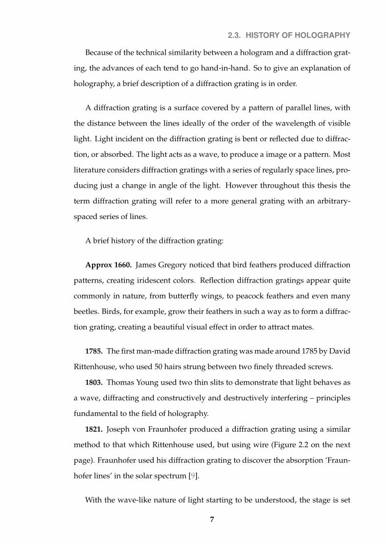
1821. Joseph von Fraunhofer produced a diffraction grating using a similar
method to that which Rittenhouse used, but using wire (Figure 2.2 on the next
page). Fraunhofer used his diffraction grating to discover the absorption ‘Fraun-
hofer lines’ in the solar spectrum [9].
With the wave-like nature of light starting to be understood, the stage is set
7

2.3. HISTORY OF HOLOGRAPHY
Figure 2.2: Wire diffraction grating, similar to that made by Fraunhofer
for invention of holography. This starts with Dennis Gabor (Figure 2.3 on the
following page) in 1947.
Dennis Gabor was a brilliant British/Hungarian scientist with an interest in
the way that light behaves. Even as a child he was fascinated by Abbe’s theory of
the microscope and by Gabriel Lippmann’s method of color photography.
Figure 2.3: Dennis Gabor
Before he had entered university, he had already repeated many modern (at
that time) experiments on wireless X-rays and radioactivity, with his brother
George Gabor.
He moved to Germany for his education, and during his time at university, he
8

2.3. HISTORY OF HOLOGRAPHY
invented one of the first high speed cathode ray oscillographs, and made the first
iron-shrouded magnetic electron lens. He worked for a while in this field, but
left Germany when Hitler came into power. He ultimately ended up in England,
and despite the depression managed to find work at a research company, British
Thomson-Houston Co., where he would work for many years.
1946. During his time at the company, Gabor et al. [10] wrote the first papers
on communication theory, as well as many other subjects. Although on the sur-
face it seems that communication theory has nothing to do with creating pretty
3D images, it actually the underlying theory of how holography works. Gabor
[11] went on to first develop stereoscopic cinematography, and then on to creat-
ing basic flat holograms – although at the time his was goal was to improve the
resolution of the electron microscope [12, 13, 14].
The first hologram made by Gabor was an in-line plane transmission holo-
gram [15]. In-line means that the reference beam and object beam come from the
same direction. This was a requirement for Gabor because his light source was a
mercury arc lamp. The light was filtered (he used the 546 nm mercury green line)
and squeezed through a pinhole to make it quasi-coherent. The resulting light
had a very small coherence length – just enough to make an in-line hologram.
A plane hologram, as opposed to a white-light hologram, means that the holo-
gram has to be reconstructed (viewed) in the same monochromatic light.
A transmission hologram is one which is viewed with a light being transmit-
ted through the hologram. The replay light (the light to view it again) has to
illuminate the hologram at the same angle, but in the opposite direction, that the
reference beam was at when exposing the hologram. The virtual image of the
object appears at the original object position. Since for in-line holograms the ob-
ject and reference beams come from the same direction, this meant that to view
Gabor’s in-line holograms, the viewing light had to be shining straight into the
9
2.3. HISTORY OF HOLOGRAPHY
viewer’s eyes, or else projected onto a surface [16]. And for Gabor, this viewing
light had to be his dim filtered mercury-arc lamp.
Despite the problems with his holograms, Gabor et al. [2] had proved that the
interference pattern carries all the information about the original object, and that
from the interference pattern you can reconstruct the entire image of the original
object. It was for these concepts that in 1971 Gabor was awarded the Nobel Prize
for Physics.
Although the first holograms were very interesting, and generated some talk
in the scientific world, Gabor was much too early. Lasers still had not been in-
vented, and the reliance on mercury arc lamps meant that it took several hours to
expose even a small hologram.
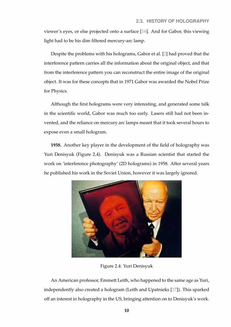
1958. Another key player in the development of the field of holography was
Yuri Denisyuk (Figure 2.4). Denisyuk was a Russian scientist that started the
work on ‘interference photography’ (2D holograms) in 1958. After several years
he published his work in the Soviet Union, however it was largely ignored.
Figure 2.4: Yuri Denisyuk
An American professor, Emmett Leith, who happened to the same age as Yuri,
independently also created a hologram (Leith and Upatnieks [17]). This sparked
off an interest in holography in the US, bringing attention on to Denisyuk’s work.
10
2.3. HISTORY OF HOLOGRAPHY
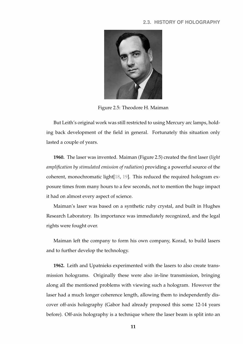
Figure 2.5: Theodore H. Maiman
But Leith’s original work was still restricted to using Mercury arc lamps, hold-
ing back development of the field in general. Fortunately this situation only
lasted a couple of years.
1960. The laser was invented. Maiman (Figure 2.5) created the first laser (light
amplification by stimulated emission of radiation) providing a powerful source of the
coherent, monochromatic light[18, 19]. This reduced the required hologram ex-
posure times from many hours to a few seconds, not to mention the huge impact
it had on almost every aspect of science.
Maiman’s laser was based on a synthetic ruby crystal, and built in Hughes
Research Laboratory. Its importance was immediately recognized, and the legal
rights were fought over.
Maiman left the company to form his own company, Korad, to build lasers
and to further develop the technology.
1962. Leith and Upatnieks experimented with the lasers to also create trans-
mission holograms. Originally these were also in-line transmission, bringing
along all the mentioned problems with viewing such a hologram. However the
laser had a much longer coherence length, allowing them to independently dis-
cover off-axis holography (Gabor had already proposed this some 12-14 years
before). Off-axis holography is a technique where the laser beam is split into an
11
2.3. HISTORY OF HOLOGRAPHY
object and reference beam. The object beam illuminates the object, and is scat-
tered onto the film. The mutually coherent reference beam is shone onto the film,
from the same side but at a different angle. The two beams interfere and the in-
terference pattern recorded. This means that on replay, the reconstructing beam
is no longer coming from the same place as the virtual object.
Leith and Upatnieks [20, 21] applied communication theory[10] and the re-
construction process of Gabor et al. [2] to produce a mathematical analysis of
wavefront reconstruction in three dimensions.
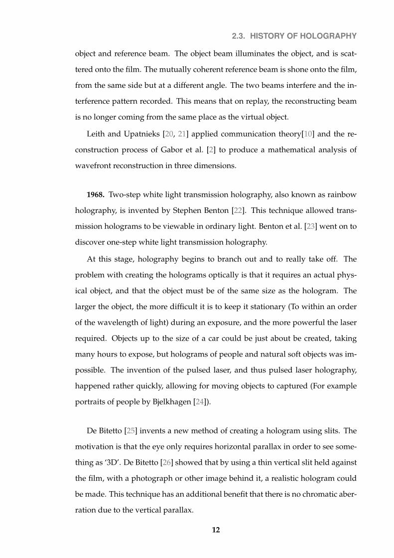
1968. Two-step white light transmission holography, also known as rainbow
holography, is invented by Stephen Benton [22]. This technique allowed trans-
mission holograms to be viewable in ordinary light. Benton et al. [23] went on to
discover one-step white light transmission holography.
At this stage, holography begins to branch out and to really take off. The
problem with creating the holograms optically is that it requires an actual phys-
ical object, and that the object must be of the same size as the hologram. The
larger the object, the more difficult it is to keep it stationary (To within an order
of the wavelength of light) during an exposure, and the more powerful the laser
required. Objects up to the size of a car could be just about be created, taking
many hours to expose, but holograms of people and natural soft objects was im-
possible. The invention of the pulsed laser, and thus pulsed laser holography,
happened rather quickly, allowing for moving objects to captured (For example
portraits of people by Bjelkhagen [24]).
De Bitetto [25] invents a new method of creating a hologram using slits. The
motivation is that the eye only requires horizontal parallax in order to see some-
thing as ‘3D’. De Bitetto [26] showed that by using a thin vertical slit held against
the film, with a photograph or other image behind it, a realistic hologram could
be made. This technique has an additional benefit that there is no chromatic aber-
ration due to the vertical parallax.
12

2.3. HISTORY OF HOLOGRAPHY
A basic holographic printer utilizing an LCD screen [27] used an optical vi-
bration isolation table with a split-beam Continuous Wave (CW) laser. The object
beam transmissively illuminates an LCD screen and projects the image onto a dif-
fusive screen. This screen acts as the object in traditional holography illuminating
the hologram plate. However only a small area of the hologram plate is illumi-
nated – the rest is blocked off with a large slit aperture. The image is changed
on the LCD screen, and another area of the hologram plate is illuminated. In this
fashion the hologram plate is exposed to multiple images – each image offering
a slightly different perspective. The images can be either taken by a camera or be
computer generated.
The mutually-coherent reference beam is arranged to simultaneously illumi-
nate the hologram plate, generating the required wave-interference spatial pat-
tern on the light sensitive emulsion. The area exposed for illumination can be
one of 2D array of rectangles/squares, producing full-parallax holograms at the
cost of longer print times, or one of a 1D array of slits, producing single-parallax
holograms.
This technique however relies on a CW laser and a diffusive screen, making it
very sensitive to vibrations.
McGrew [28] side steps the need for a diffusion screen by directly exposing
the laser light onto the holographic plate. But this still suffers from vibration
problems.
1969. Benton develops the rainbow hologram, requiring two recording steps
(termed two-step holography). A master hologram is recorded from a real object
with conventional off-axis holographic techniques. The rainbow hologram is then
recorded from the image of the master [27].
The technique of recording a master hologram offers a significant advantage;
it allows for the mass production of the rainbow hologram without the phys-
ical object, making commercial holography a real possibility. Commercial ma-
13
2.3. HISTORY OF HOLOGRAPHY
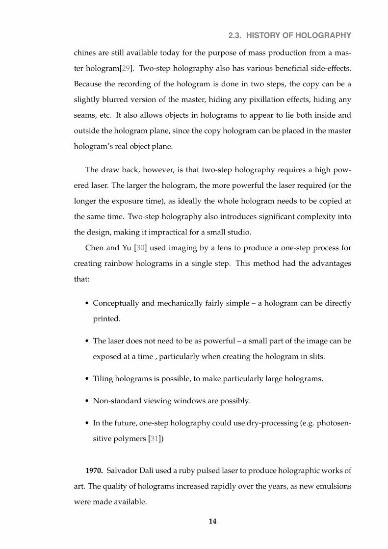
chines are still available today for the purpose of mass production from a mas-
ter hologram[29]. Two-step holography also has various beneficial side-effects.
Because the recording of the hologram is done in two steps, the copy can be a
slightly blurred version of the master, hiding any pixillation effects, hiding any
seams, etc. It also allows objects in holograms to appear to lie both inside and
outside the hologram plane, since the copy hologram can be placed in the master
hologram’s real object plane.
The draw back, however, is that two-step holography requires a high pow-
ered laser. The larger the hologram, the more powerful the laser required (or the
longer the exposure time), as ideally the whole hologram needs to be copied at
the same time. Two-step holography also introduces significant complexity into
the design, making it impractical for a small studio.
Chen and Yu [30] used imaging by a lens to produce a one-step process for
creating rainbow holograms in a single step. This method had the advantages
that:
• Conceptually and mechanically fairly simple – a hologram can be directly
printed.
• The laser does not need to be as powerful – a small part of the image can be
exposed at a time , particularly when creating the hologram in slits.
• Tiling holograms is possible, to make particularly large holograms.
• Non-standard viewing windows are possibly.
• In the future, one-step holography could use dry-processing (e.g. photosen-
sitive polymers [31])
1970. Salvador Dali used a ruby pulsed laser to produce holographic works of
art. The quality of holograms increased rapidly over the years, as new emulsions
were made available.
14
2.3. HISTORY OF HOLOGRAPHY
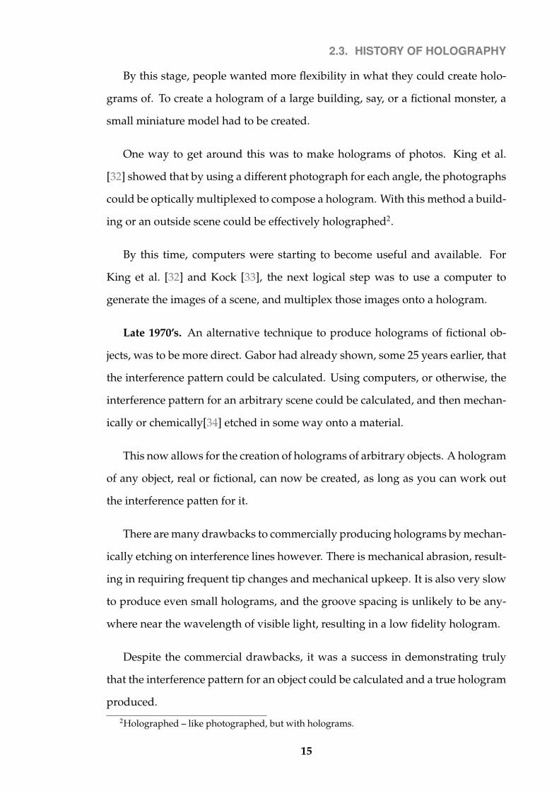
By this stage, people wanted more flexibility in what they could create holo-
grams of. To create a hologram of a large building, say, or a fictional monster, a
small miniature model had to be created.
One way to get around this was to make holograms of photos. King et al.
[32] showed that by using a different photograph for each angle, the photographs
could be optically multiplexed to compose a hologram. With this method a build-
ing or an outside scene could be effectively holographed2.
By this time, computers were starting to become useful and available. For
King et al. [32] and Kock [33], the next logical step was to use a computer to
generate the images of a scene, and multiplex those images onto a hologram.
Late 1970’s. An alternative technique to produce holograms of fictional ob-
jects, was to be more direct. Gabor had already shown, some 25 years earlier, that
the interference pattern could be calculated. Using computers, or otherwise, the
interference pattern for an arbitrary scene could be calculated, and then mechan-
ically or chemically[34] etched in some way onto a material.
This now allows for the creation of holograms of arbitrary objects. A hologram
of any object, real or fictional, can now be created, as long as you can work out
the interference patten for it.
There are many drawbacks to commercially producing holograms by mechan-
ically etching on interference lines however. There is mechanical abrasion, result-
ing in requiring frequent tip changes and mechanical upkeep. It is also very slow
to produce even small holograms, and the groove spacing is unlikely to be any-
where near the wavelength of visible light, resulting in a low fidelity hologram.
Despite the commercial drawbacks, it was a success in demonstrating truly
that the interference pattern for an object could be calculated and a true hologram
produced.
2Holographed – like photographed, but with holograms.
15

2.3. HISTORY OF HOLOGRAPHY
Briefly looking at the next twenty years of development in holography field:
1979. McGrew [35], working with the Diffraction Company, develops an em-
bossing mass production technique for surface relief holograms. McGrew went
on to form his own company, Light Impressions Inc, which was the first company
to bring the embossed hologram to the commercial market with a set of embossed
images of 3D subjects.
Early 1980’s. Benton proposes the use of a movie camera mounted on a linear
rail to obtain images of on object at different angle, as opposed to rotating object
on turn table[36].
1988. F. Iwata and K. Ohuma, of Toppan Printing Co Ltd, made a novel pro-
cess for making animated diffractive patterns by making lots of small tiny dots
of gratings. Although crude, it is effective. It allows for very fine diffraction grat-
ings, giving a high efficiency, while maintaining a crude control of the image (by
deciding whether to put a dot in a particular place, etc.)
Davis [37] and Newswanger [38] independently improved on this by modu-
lating the object, allowing crude 3D images to be built up of ‘pixels’.
This thesis follows a similar method as pioneered by Davis and Newswanger
– building up a hologram by printing in a ‘dot matrix’ style of ‘pixels’ in a grid.
Throughout this thesis, the printed ‘pixels’ on the hologram will be referred to as
as holopixels, to emphasize their iridescent nature.
1992. By the early 1990’s, computers and LCD screens were a lot more ubiqui-
tous. Spierings and Nuland [39] replaced film in their Holoprinter with an LCD
screen. Nuland and Spierings [40] went one step further over the course of a year,
and make color 3D stereograms using an LCD in a single step
1994. Yamaguchi et al. [41, 42] describes a monochrome one-step holographic
printer based on a CW laser. This can print small full parallax white-light reflec-
16
2.4. DIGITAL VERSUS ANALOGUE
tion holograms, but takes 2 seconds per pixel – e.g. 36 hours to do a reflection
hologram of 320x224 holopixels.
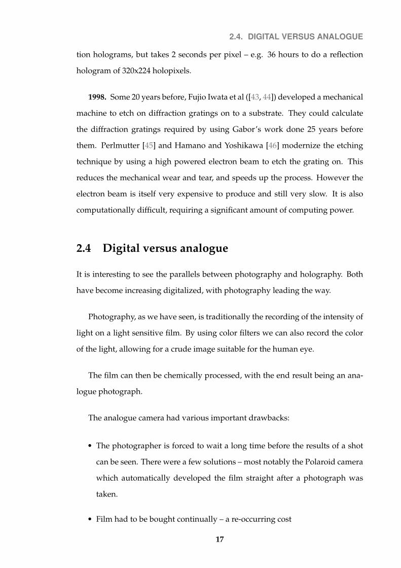
1998. Some 20 years before, Fujio Iwata et al ([43, 44]) developed a mechanical
machine to etch on diffraction gratings on to a substrate. They could calculate
the diffraction gratings required by using Gabor’s work done 25 years before
them. Perlmutter [45] and Hamano and Yoshikawa [46] modernize the etching
technique by using a high powered electron beam to etch the grating on. This
reduces the mechanical wear and tear, and speeds up the process. However the
electron beam is itself very expensive to produce and still very slow. It is also
computationally difficult, requiring a significant amount of computing power.
2.4 Digital versus analogue
It is interesting to see the parallels between photography and holography. Both
have become increasing digitalized, with photography leading the way.
Photography, as we have seen, is traditionally the recording of the intensity of
light on a light sensitive film. By using color filters we can also record the color
of the light, allowing for a crude image suitable for the human eye.
The film can then be chemically processed, with the end result being an ana-
logue photograph.
The analogue camera had various important drawbacks:
• The photographer is forced to wait a long time before the results of a shot
can be seen. There were a few solutions – most notably the Polaroid camera
which automatically developed the film straight after a photograph was
taken.
• Film had to be bought continually – a re-occurring cost
17

2.4. DIGITAL VERSUS ANALOGUE
• Negatives also had to be stored along with the photographs in case reprints
were needed at a later time.
There are many other factors to consider, and the debate between analogue
and digital photography is still ongoing today.
The 1990s saw the advent of digital photography. Digital photography al-
lowed for photographs to be captured with CCD based image sensors. The pho-
tographs could be modified and then printed to paper if needed.
18

3Design of a digital hologram printer
This chapter considers the technical design of a digital hologram printer, begin-
ning with a description of the optical and mechanical components for both the
object and reference beam paths. The lens systems in the object beam are ex-
amined quantitatively, concluding with a straightforward set of instructions for
adjusting the lens system. The chapter finishes with a qualitative examination of
the lens system based on testing three different lens arrays.
3.1 Overview
Detailed is a digital hologram printer capable of recording transmission or reflec-
tion holograms in an off-axis geometry for subsequent developing and bleaching
in order to produce white-light viewable holograms. The printer consists of: a
pulsed laser source arranged to produce a visible-light laser beam; a lens sys-
tem to direct each beam pulse to a photosensitive medium; a display system to
19

3.1. OVERVIEW
modulate the object beam; a two dimensional positioning track to position the
photosensitive medium relative to said lens system; and a computer control sys-
tem.
The use of a pulsed laser offers the advantage of printing without sensitivity
to vibrations or slight temperature changes. The printer utilizes a long-cavity
frequency-doubled Neodymium Doped Yttrium Aluminum Garnet (Nd:YAG)
pulsed laser which can produce a stable second harmonic TEM00 coherent 532 nm
(visible green) beam.
The lens system splits the beam with a Brewster-angle polarising beam splitter
into the mutually-coherent object and reference beams. The display system is a
reflective LCOS display or a transmissive LCD, placed downstream of the object
beam, and upstream of the photosensitive medium.
The use of a reflective LCOS as the display system for a hologram printer is
particularly advantageous. The high efficiency and high contrast, compared to
the less efficient transmissive LCD, allows ultimately for higher contrast upon
hologram replay and increased energy economy during writing, allowing for a
less powerful laser source to be used. The high resolution on the LCOS allows for
the hologram to have a large depth of view.
Typically a silver halide green-light photosensitive emulsion on a glass sub-
strate is placed upsteam in the Fourier plane of the display system, recording
the spatial standing diffraction pattern between the reference and object beams.
This records a small ‘pixel’ of the order of 1 mm in diameter. The motorized two-
dimensional positioning tracks translate the plate into position for the next pixel
to be printed. The plate can then be developed and bleached chemically to pro-
duce a white-light viewable reflection hologram.
The hologram printer design outlined in this chapter is based upon the digital
hologram printer detailed by Ratcliffe et al. [47]. The patent consists of the gen-
eral schematic for a monochromatic hologram printer, but lacks key information
required for implementation and modification. As is typical for any complicated
20

3.1. OVERVIEW
machine, intricate knowledge is required for correct fabrication; alignment mis-
takes will result in a bad hologram (e.g. containing dim, missing or bad pixels).
Because of the design’s sensitivity to the layout, a methodical and detailed
setup that incorporates previous experience is required. The patent also misses
vital theoretical information required for modifying the machine. The lens system
used around the microlens array and display system is sensitive to position. This
chapter details the setup required to produce high-fidelity images while wasting
the minimum amount of energy and controlling the energy density and pixel size
of the beam exposed to the holographic plate. This is accomplished with a mix of
quantitative and qualitative analysis of the lens system.
The basis of this work is the green pulsed-laser holographic printer detailed
by Ratcliffe et al. [47] and illustrated in Figure 3.1 on the next page. The said holo-
gram printer can print 1.0 mm×1.0 mm sized pixels onto a photosensitive glass
plate at a maximum rate of 4 pixels per second. The majority of the energy from
the laser is lost at various points in the design. The mechanical setup suffered
from mechanical vibrations. The laser was also unstable with between 10% to
30% pulse-to-pulse variation in energy. This produces noticeable changes in the
hologram. The goal of the work reported was to overcome these shortcomings,
increase the printing speed and decrease the pixel size.
21

3.1. OVERVIEW
Figure 3.1: Hologram printer with LCD display system by Ratcliffe et al. [47]. Forfull-page schematics, see also Figure C.2 on page 155 and Figure C.1 on page 154.
22
3.2. DETAIL OF SYSTEM COMPONENTS
3.2 Detail of system components
This section provides a detailed description for the building of digital hologram
printer for writing composite 1-step holograms.
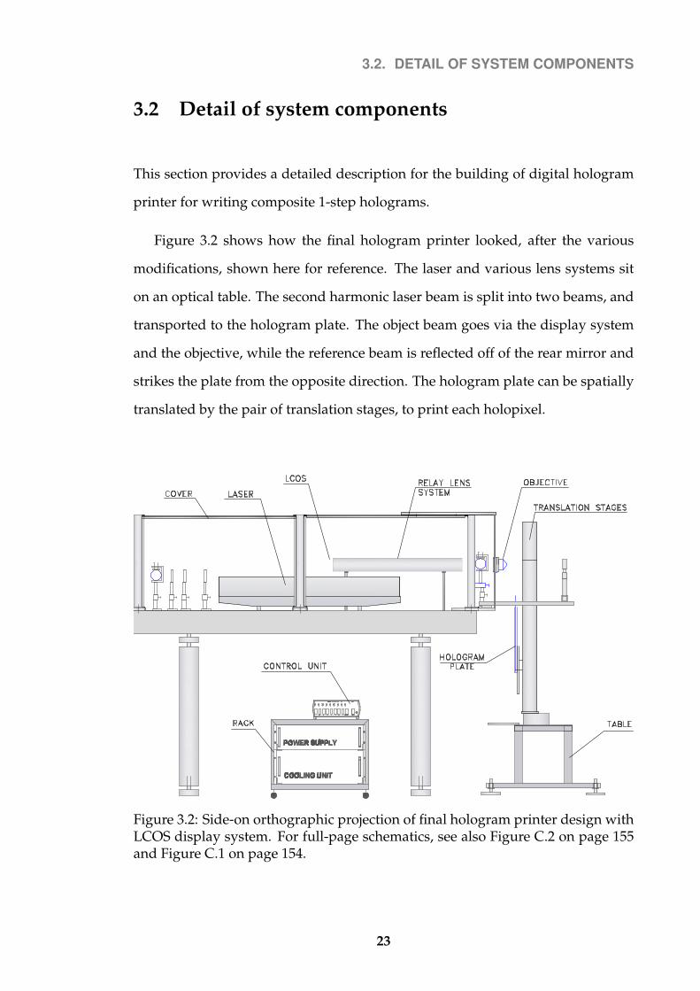
Figure 3.2 shows how the final hologram printer looked, after the various
modifications, shown here for reference. The laser and various lens systems sit
on an optical table. The second harmonic laser beam is split into two beams, and
transported to the hologram plate. The object beam goes via the display system
and the objective, while the reference beam is reflected off of the rear mirror and
strikes the plate from the opposite direction. The hologram plate can be spatially
translated by the pair of translation stages, to print each holopixel.
Figure 3.2: Side-on orthographic projection of final hologram printer design withLCOS display system. For full-page schematics, see also Figure C.2 on page 155and Figure C.1 on page 154.
23

3.2. DETAIL OF SYSTEM COMPONENTS
Figure 3.3: Top-down orthographic projection of final hologram printer designwith LCOS display system. For full-page labelled schematics see also Figure C.3on page 156 and Figure C.4 on page 157.
3.2.1 Laser system
Most lasers will rest on their own bread board which in turn stands on legs. The
height of the laser can be adjusted; however it is a lot more flexible to adjust the
height of the beam by using a system of mirrors instead.
The object beam is raised to the correct height using a triangle of three mirrors,
each higher than the last. The beam then passes through a motorized half wave
plate which rotates the polarization. The beam then passes through a Brewster-
angle split beam polariser. The p-component of the laser light is transmitted
through the split-beam polariser, while the s-component is reflected.
It is very important to get the angle of the Brewster polariser correct, other-
wise circular polarization of the beam will result. To align correctly, the angle of
the ½-wave plate is set to maximize the amount of reflected light (so that it po-
larises the light into the p-direction). This is best done by using an energy meter
to measure the intensity of the light reflected from the split-beam polariser. By
eye, check the profile of the transmitted beam is then checked. If the angle of the
split beam polariser is wrong, the beam profile will look poor. The angle of the
24

3.2. DETAIL OF SYSTEM COMPONENTS
split-beam polariser is adjusted to minimize the intensity of the transmitted beam
and produce a good Gaussian beam profile. In this setup the Brewster split beam
polariser was coated with an anti-reflection surface, increasing the efficiency. For
a non-coated split-beam polariser it is possible that the maximum transmitted
energy is not at the Brewster angle [48]. In this case, the best results would prob-
ably be obtained by trying to maximise the quality of the beam, rather than the
intensity.
3.2.2 Optics for transport of beams
Adjustable object beam path length
Figure 3.4 shows that the object beam is reflected between two sets of mirrors,
with one set of mirrors mounted on a sliding base. This allows the distance be-
tween the two sets of mirrors (and hence the overall optical path length of the
object beam) to be easily adjusted, while keeping the correct beam alignment.
Figure 3.4: Top-down orthographic projection of system to adjust optical-pathdistance of object beam. See also Figure C.5 on page 158 for a full-page schematic.
25

3.2. DETAIL OF SYSTEM COMPONENTS
It is important to be able to modify the object beam path length such that the
difference in distance travelled by the reference beam and object beam is kept as
small as possible. This maximises the temporal overlap of the object and refer-
ence beam pulses at the hologram plate. If one beam arrives at the plate before the
other, it will expose the plate without any signal, reducing contrast and diffrac-
tion efficiency upon replay.
To setup this system of mirrors, all four mirrors were mounted as indicated,
with two of the mirrors on a sliding base. The base was moved back and forth
while watching for beam movement. The angles of the four mirrors were ad-
justed until there was no perceptible lateral movement of the beam when the
base is moved.
Cleaning up the object beam
To produce a clean Gaussian spatial profile of the object (and reference) beam if
required, a pair of positive lenses (Marked L5 and L6 in Figure 3.4 on the preced-
ing page) placed at a distance equal to the sum of their focal lengths can be used,
with a pinhole aperture (not shown) placed at the their mutual focusing plane to
remove any high order defects. This afocal lens system can have the dual purpose
of magnifying the beam as required, where there magnification of the laser beam,
Mlaser is dependant on the focal length of L5, fL5 and the focal length of L6, fL6 as:
Mlaser =fL5
fL6(3.1)
The beam can thus be magnified such that its diameter closely matches the
downstream width of object beam aperture, to maximise overall beam efficiency.
3.2.3 Digital display system
In direct write analogue holography, the object beam illuminates a physical ob-
ject. The illuminated beam is reflected off of the object, modulated by the object,
26
3.2. DETAIL OF SYSTEM COMPONENTS
and may be considered to scatter as a series of spherical waves. A photosensitive
plate is positioned as to capture this light. A reference beam, also incident upon
the plate, interferes with the modulated object beam creating a microscopic inter-
ference pattern (fringe pattern) that encodes the required information about the
object. This fringe pattern is recorded on to the plate as an absorption hologram,
to be developed and bleached to create a white light hologram. On replay of the
hologram, the object image is reconstructed in its original position.
For digital holography the physical object is replaced with a computer con-
trolled display system. This ultimately allows the production of a hologram us-
ing a computer generated model or a series of photographs or some other method
that generates a series of suitable images. There are various methods for using a
computer controlled display.
The display system used was a LCOS based Spacial Light Modulator (SLM);
a small, reflective, high contrast, high fill-rate and high resolution panel. This has
the advantages of a small form factor allowing for future miniaturization of the
printer; high resolution allowing for holograms with a large depth of field (both
in and out of the hologram plane); high efficiency rate increasing overall beam
efficiency and allowing for a weaker laser to be used, thus decreasing the cost and
increasing the lifetime of the printer; high contrast which in turn allows for high
contrast holograms; and a high fill rate of up to 60 Hz, allowing for holograms to
be printed at up to this rate of holopixels per second.
Figure 3.5 on the next page illustrates the logical layout required and Fig-
ure 3.6 on page 29 is a photograph of the microlens array system downstream of
the LCOS.
27

3.2. DETAIL OF SYSTEM COMPONENTS
Optical Fourier transform
xlcos
ylcos
LCOS
xhologram
yhologram
z
eye
viewing window
Figure 3.5: The Fourier transform of the image on the LCOS is printed on to thehologram as a single ’holopixel’. Upon replay of the hologram, this recordedFourier image is reconstructed as an angular intensity distribution.
28

3.2. DETAIL OF SYSTEM COMPONENTS
Figure 3.6: Birds-eye-view photograph of LCOS being illuminated, with the beampath indicated.
29

3.3. ANALYSIS OF LENS SYSTEM
3.3 Analysis of lens system
The object beam is shaped according to several restrictions. The requirements are
that:
• The beam exposes the LCOS uniformly and smoothly.
• Energy losses are minimized – the beam should illuminate the whole of the
LCOS display while minimizing losses. Thus the beam profile should be
rectangular and of the same aspect ratio and scale.
• The spatial profile of the beam at the plane of the hologram plate emul-
sion should be of a controllable size and shape. Typically either circular or
square with a width of around 1 mm to 0.3 mm.
To achieve these aims, an afocal reversing telescopic lens system with an objec-
tive compound lens was designed and optimized using the lens software ZEMAX
[49]. The lenses were designed and built by Marcin Lesniewski. The resulting
setup is shown in Figure 3.7 on the next page.
The object beam is spatially filtered by the rectangular aperture P which has
an aperture width y, as labelled in Figure 3.7 on the following page. The shape of
the aperture will ultimately determine the downstream beam’s spatial geometry
(scaled in size by a factor 1/M3) of the pixel in the real image plane I1 and the real
image labelled I3 where the photosensitive plate is placed.
The beam travels the distance labelled z to the microlens array A. This is a
rectangularly-packed microlens array with spherically curved lenslets. The plane
geometry of the lenslets in the microlens array determines the spatial shape of
the beam on the LCOS display. Since the LCOS display system is rectangular, the
lenslets are also chosen to be rectangular, with the same aspect ratio.
30

3.3. ANALYSIS OF LENS SYSTEM
Figure 3.7: Top-down orthographic projection of object lens system in hologramprinter. See also Figure C.6 on page 159 for a full-page schematic.
The expanded beam enters the positive lens L1 downstream of the microlens
array, is reflected off the right-angled coated mirror, and continues to the polaris-
ing beam splitter.
The beam’s polarization is already orientated in the direction such that all of
the beam’s energy is directed by the polarizing beam splitter to the LCOS display
system. The lenses between the microlens array and LCOS are arranged such that
the beam arrives at the display system with the correct spatial geometry and scal-
ing to match the display region on the LCOS. Preferably the beam should have
an even spatial beam intensity profile with minimal defects and speckle in order
to produce a replay viewing window with an even intensity. It is conceivable
to desire a non-even beam distribution (for example Gaussian) for the purpose
of having a brighter optimal replay angle at the sacrifice of dimmer non-optimal
replay angles. Such possibilities are not considered further here, and an even
spatial beam intensity profile is assumed to be desired.
31

3.3. ANALYSIS OF LENS SYSTEM
The LCOS twists the polarization of the light at each pixel, to build up a spatial
image. For a full intensity pixel, the polarization is rotated 90 degrees. For a black
pixel, the polarization is not rotated. For greyscale, it is only partially rotated.
A thin weak lens in front of the LCOS display acts as a field lens to correct
for the final image curvature so that the final image from the objective lens L4 is
focused on a flat plane. A schematic for the physical mount for the LCOS display,
field lens and beam splitter is given in Appendix F, Figure F.1 on page 167. The
light beam, now containing the image that was on the LCOS, is now reflected
back through the split beam polarising cube, splitting the image into an intensity
encoded image and its negative. The negative bounces back along the original
path, harmlessly being ignored. The positive image is then sent through a custom
LCOS telecentric afocal reversing lens system to be projected on to the hologram
plate.
The purpose of the LCOS lens system is to project the image of the LCOS onto
a virtual hemisphere, mapping the two dimensional pixel spatial coordinates to
longitude and latitude spherical coordinates, projected on to the holographic film.
Upon replay of the final developed hologram, each holographic pixel is iri-
descent – the brightness of the pixel changes with the angle at which it is viewed
from, with the angular intensity profile matching the original spatial pattern that
was on the LCOS.
This projection from the flat spatial plane (I1) at the LCOS to a hemispherical
plane at the hologram plate (I3) is achieved with the telescopic afocal reversing
lens system and objective lens. This lens setup is shown in Figure 3.8 and Fig-
ure 3.9 on the following page, with sample ray-traced light paths overlaid on the
figure.
32
3.3.A
NA
LYS
ISO
FLE
NS
SY
STE
M
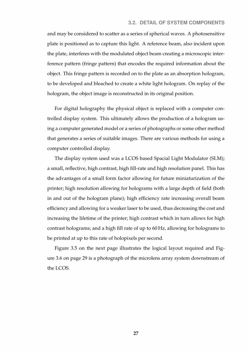
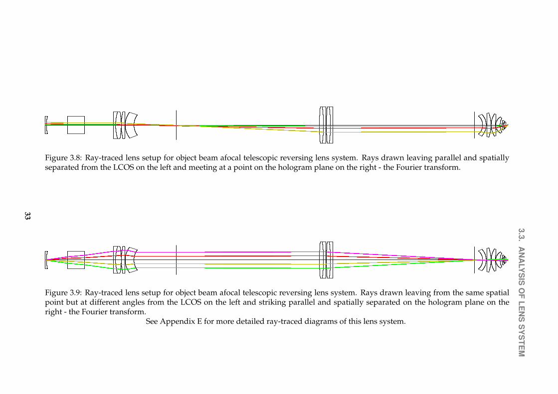
Figure 3.8: Ray-traced lens setup for object beam afocal telescopic reversing lens system. Rays drawn leaving parallel and spatiallyseparated from the LCOS on the left and meeting at a point on the hologram plane on the right - the Fourier transform.
Figure 3.9: Ray-traced lens setup for object beam afocal telescopic reversing lens system. Rays drawn leaving from the same spatialpoint but at different angles from the LCOS on the left and striking parallel and spatially separated on the hologram plane on theright - the Fourier transform.
See Appendix E for more detailed ray-traced diagrams of this lens system.
33

3.3. ANALYSIS OF LENS SYSTEM
This complex system of lenses provides near diffraction-limited optical per-
formance, requiring various different optical elements and several different glass
materials to correct for various aberrations.
It is, however, desirable to derive a simple set of formulas that describes this
lens system. This allows us to determine the effect of the set up of the optical
system downstream, on the holopixel that is projected upstream. The size and
shape of the final holopixel is determined by both the downstream lens system as
well as the telescopic afocal lens system. The lens system was previously set up
by a method of trial and error. This can produce adequate results for printing at
large pixel sizes, however it is prone to error and makes it difficult to know what
the ultimate holopixel size will be for a given lens setup.
For a large holopixel size (around 1 mm), setting up the lens system by eye is
feasible and provides results of sufficient quality. However for smaller holopixel
sizes (less than 0.5 mm), the system becomes increasingly sensitive to the exact
placement of the lenses. Large uncertainties in the beam size translate to large
uncertainties in the energy density on the photographic plate. Finding a ’sweet
spot’ for the correct pixel size and pixel fidelity frequently results in the beam size
exceeding that of the optics, resulting in undesirable energy losses.
The purpose of this section is to provide an analytical approach to the prob-
lem. To do this, the telecentric afocal reversing lens system is treated as two
overlapping relay telescopes. The compound lenses are ray-traced to determine
their effective focal lengths. The small weak lens on the LCOS is a field lens for
correcting the curvature on the final image, and is thus assumed to be negligible
for these purposes.
Since the vertically polarised (the negative) part of the image from the LCOS is
discarded by the polarised beam splitter, the phrase ‘LCOS image’ will be used to
mean the reflected horizontally-polarised image (the positive), in order simplify
the language required.
34

3.3. ANALYSIS OF LENS SYSTEM
Consider the image from the LCOS passing through the beam splitter and
then continuing through the lens L2. It forms a real image at I1. By considering
that L2 and L1 approximately form a relay lens system, it can be seen that the
image at L1 will be that of the aperture P, scaled according to the lens relay for-
mulas (considered later). The beam continues through L3, forming an image at
I2. By considering that the lenses L3 and L2 form a relay lens, it can be seen that
this image at I2 is the image of the LCOS, again scaled according to the lens relay
formulas.
The system of lenses at L4 take the image at I2 and focus it at I3 which is thus
the Fourier transform plane for the lens system L4. By considering that L4 and
L3 form a relay lens, it can be seen that this image at I3 is the image that was at
I1, and thus is an image of the aperture P, scaled twice by the two sets of relay
lenses. The details of the lens are discussed in more detail later in Section 3.3.5 on
page 40.
The image at I3 has a geometrically similar shape (i.e. the same shape but
scaled) to that of that of P. It is also the Fourier transform of the image I2.
The thin lens formula in air is:
1
S1
+1
S2
=1
f(3.2)
Where S1 is the distance between an object plane and a thin lens with focal
length f and S2 is the distance between the thin lens and the image plane.
For two thin lenses with focal lengths f1 and f2 respectively, separated by an
optical distance of f1+f2 , the final convergence of the beam is not altered (making
it afocal), but the width of the beam is magnified by a factor of:
M = −f1
f2
(3.3)
Thus the object image plane at distance f1 from the first lens will be relayed to
the image plane at distance f2 from the second lens and inverted.
35

3.3. ANALYSIS OF LENS SYSTEM
Compound lenses have a front focal length and a back focal length. The front
focal length is the distance from the front surface to the principle upstream focal
point. The back focal length is the distance from the back surface to the principle
downstream focal point. While this is important for the placement and design of
the compound lens, for the purposes of determining the magnification, the front
and back focal lengths are not of particular interest.
The effective focal length for a compound lens is the distance from a principle
plane to its corresponding principle focal point[50].
So if lens 1 has an effective focal length f1 and is downstream of lens 2 which
likewise has an effective focal length f2, and if their inner principle planes are
separated by a distance of f1 + f2 then the image plane at a distance f1 from back
principle plane of lens 1 is magnified at the image plane at a distance f2,f from
the front principle lane of lens 2 by a factor of:
M = −f1
f2
(3.4)
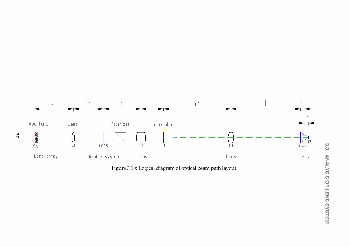
The object beam lens system is shown schematically in Figure 3.10 on the fol-
lowing page. Note that the actual path of the laser beam from lens L1 to the LCOS
is via a mirror and the beam splitter. For diagram simplicity it is drawn as if the
LCOS is transmissive. The distance labelled b should be interpreted as the optical
distance from L1 to the LCOS.
Note that L2, L3 and L4 are compound lenses with different front and back fo-
cal distances. As is the convention in optics, the front is defined as in the direction
of the beam, and back as the direction in which the beam came from.
This complex system of lenses is particularly sensitive to distances between L1
and L3, requiring an optical collimator for precise alignment. This can be done by
mounting the LCOS and its weak correctional mirror together onto the moving
platform at one end.
36
3.3.A
NA
LYS
ISO
FLE
NS
SY
STE
M
Figure 3.10: Logical diagram of optical beam path layout
37

3.3. ANALYSIS OF LENS SYSTEM
3.3.1 Lenses L1 and L2
The object image plane at aperture P is at a distance of a from the center of lens
L1, which has a effective focal length of f1. The distance from the aperture P to
the closest principle plane of lens L1 should be approximately equal to the focal
length, not exactly, such that the final pixel shape is a slightly defocused image of
the aperture, producing a blurred outline on the hologram film.
The light then travels a total distance of b + c to lens L2, via a mirror, beam
splitter, a reflection off of the LCOS, twice passing through a small correction field
lens on the LCOS, and back through the beam splitter.
The lenses L1 and L2 act together as an afocal relay lens, imaging the aperture
P at the image plane I1.
It turns out that it is sufficient to use a thin lens at L1. Thus the principle
plane is at the center of L1. The magnification due to L1 and L2, MP,1, can be
determined, given that the effective focal length of lens L2 is f2.
f1 ≈ a (3.5)
f1 = b (3.6)
MP,1 = −f1
f2
(3.7)
3.3.2 Lenses L3 and L4
The lenses L3 and L4, with effective focal lengths f3 and f4 respectively, likewise
act together as an afocal relay lens, imaging the image of the aperture P at I1 to
the image plane I3. The image plane I1 is magnified by a factor of M1,3 = −f3
f4at
image plane I3.
The image plane P is magnified by a factor of −f1
f2at the real image plane I1,
and then magnified again by a factor of−f3
f4at the real image plane I3. So the total
38

3.3. ANALYSIS OF LENS SYSTEM
magnification, MP,3 of the aperture P at the image plane I3 is:
MP,3 =f1f3
f2f4
(3.8)
So the shape and size of P determines the shape and size of the final holopixel
on the holographic film plate, magnified by a factor M3. The Zemax software
determined the effective local length of the system from the LCOS display to the
lens L4 to be feff = −7.669 mm. Thus:
MP,3 = − f1
feff(3.9)
MP,3 = − f1
−7.669 mm(3.10)
=f1
7.669 mm(3.11)
3.3.3 Lenses L2 and L3
For completeness, consider the lens system formed by L2 and L3. The image
plane of the LCOS is relayed to the image plane I2 by lenses L2 and L3 with effec-
tive focal lengths f2 and f3 respectively. The image plane I2 has a magnification
Mlcos,2 of:
Mlcos,2 = −f2
f3
(3.12)
39

3.3. ANALYSIS OF LENS SYSTEM
3.3.4 Focal length approximations
The surface properties of the compound lenses L2, L3 and L4 were calculated and
optimized in the Zemax optics software1. Table G.1 on page 169 in Appendix G
details the lens materials, separation and clear diameter properties.
For lenses L2 and L3, the effective focal length of each of the lenses can be de-
termined from the ray transfer matrices method (See Chartier [1, pages 120-130]
and the Chapter Nomenclature on page xxi). Compound lens L4 is significantly
more complex and has a much shorter focal length. As a result, the paraxial
approximation is not valid for this lens, resulting in inaccuracies in the matrix
method. The matrix method calculates the effective focal length of lens L4 to be
19.7 mm, whereas a geometrical calculation based on a raytrace produced by Ze-
max gives the effective focal length as 16.2 mm. This is shown in Figure 3.11 on
the following page. To avoid such inaccuracies, the values calculated by Zemax
were used exclusively.
3.3.5 Optical system for microlens array
There are additional factors to be taken into account because of the microlens
array close to, and downstream of, the object beam aperture. Without the mi-
crolens array, the LCOS display would be illuminated with the ‘raw’ Gaussian
beam. This means that any dust etc that was on any of the mirrors would appear
as dark spots on the LCOS along with diffraction rings. The use of a microlens
array acts a series of point sources which expand and overlap downstream, spa-
tially averaging out the noise in the beam. The microlens array is also used to
apodize2 the beam’s Gaussian spatial intensity profile into an even spatial inten-
sity profile at the LCOS display.
Unfortunately the use of a microlens array introduces an additional problem
1The Zemax software is owned by the ZEMAX Development Corporation [49] company andis used to aid in lens design.
2apodize – to purposely change the input intensity profile
40
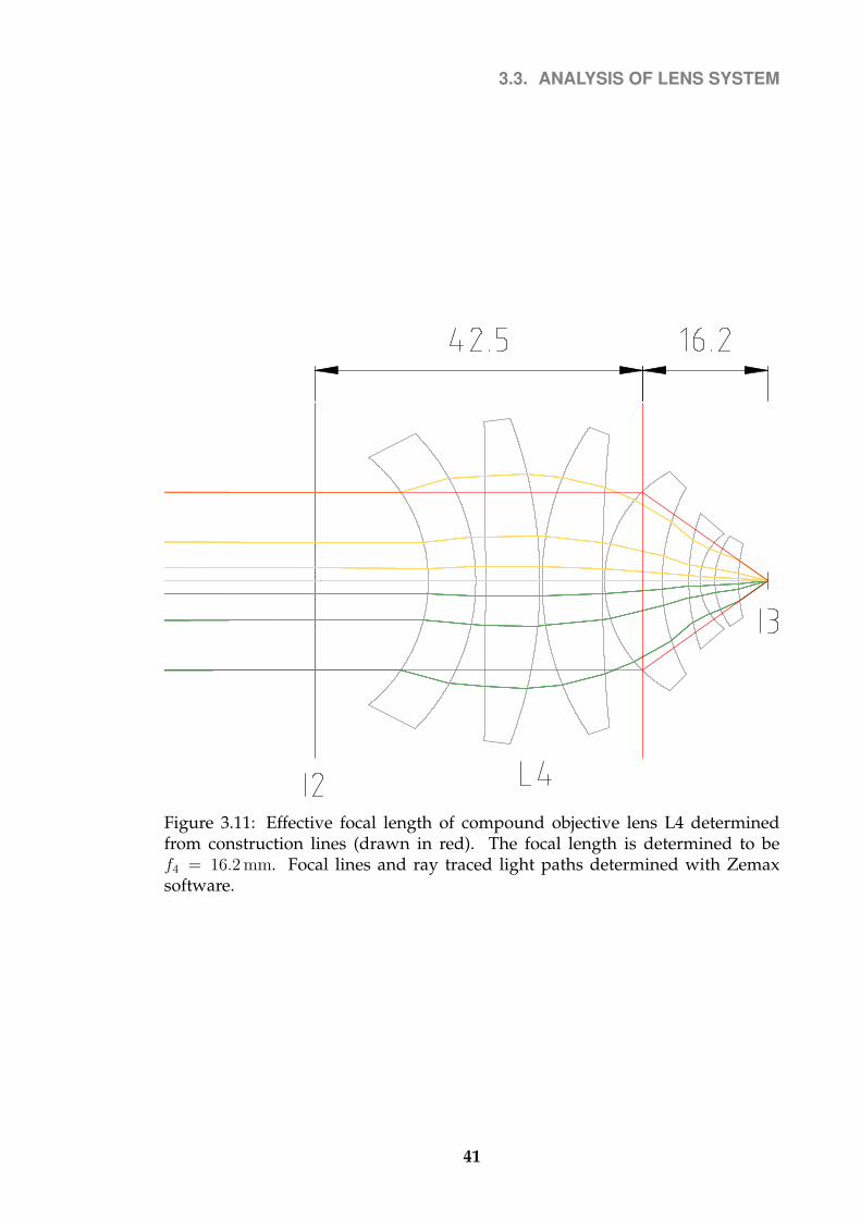
3.3. ANALYSIS OF LENS SYSTEM
Figure 3.11: Effective focal length of compound objective lens L4 determinedfrom construction lines (drawn in red). The focal length is determined to bef4 = 16.2 mm. Focal lines and ray traced light paths determined with Zemaxsoftware.
41
3.3. ANALYSIS OF LENS SYSTEM
– the overlapping beams are coherent with each other and so interfere, giving
a real speckled image. This speckle degrades the image of the LCOS and thus
reduces the effective resolution. This will reduce the overall depth of field of the
hologram when viewed.
The microlens arrays required in this design are rectangularly packed with an
aspect ratio equal or close to that of the LCOS such that the downstream beam is
similar is shape and size to the LCOS display. This rotationally asymmetric ge-
ometry results in rotationally asymmetric speckle. Rectangular speckle structures
are observed in the downstream spatial profile.
In order to analyze the microlens array system, consider the meridional plane
only (the vertical plane that crosses through the optical axis). The lenslets have
the same aspect ratio as the LCOS and the size of the beam (as we will see later)
will be a linear function of the lenslet size, so the beam will have the correct width
if the height is correct.
The Gauss conditions will also be assumed and applied – that the beam is
parallel to the optics. The assumption that the lenses are thin lens and that the
angles are small enough that sin(x) ≈ x will also be used.
First consider light rays travelling near the optical axis such that the rays pass
through a lenslet centered on the optical axis. The ray passes through this central
lenslet which has a focal length of flenslet. The ray then travels a distance of a (see
Figure 3.10 on page 37), passing through the lens L1 which has a focal length of
f1. The ray then travels a distance of b to illuminates the LCOS display. Using the
thin lens approximation and the paraxial approximation, the matrix method can
be used to examine this system (See Chartier [1, pages 120-130] and the Chap-
ter Nomenclature on page xxi). Thus using a combination of lens and transfer
matrices the path of the rays travelling through the central lenslet onto the LCOS
can be described.
The matrix method requires an input ray, vlenslet, which can be described as
42

3.3. ANALYSIS OF LENS SYSTEM
vlenslet = (r, θ)T where 2r is the height and θ is the angle that the ray is travelling
from the horizontal. The resulting ray vector on the LCOS is thus M lenslet · vlenslet,
where the matrix M for this system is thus:
M lenslet =
1 b
0 1
1 0
− 1
f1
1
1 a
0 1
1 0
− 1
flenslet1
(3.13)
This can be extended to work for an arbitrary lenslet on the lensarray, by sim-
ply extending the ray vector as:
vlensarray =
(r θ s
)T
(3.14)
Where r is the height, s is the height from the center of the lenslet that it is passing
through, and θ is the angle that the ray is travelling from the horizontal.
Only the lenslet matrix is concerned with the d parameter so this parameter is
dropped by the lensarray matrix.
The final matrix for the ray path from the lensarray to the LCOS, M lensarray,
becomes:
M lensarray =
1 b
0 1
1 0
− 1
f1
1
1 a
0 1
1 0 0
0 1 − 1
flenslet
(3.15)
From the matrix method[1], M lensarray · vlensarray = vlcos where vlcos is the ray
vector at the LCOS. Solving:
r −(a+ b) · sflenslet
− b · rf1
+a · b · sflenslet · f1
a · sflenslet · f1
− r
f1
− s
flenslet
=
rLCOS
θLCOS
(3.16)
For the image of the aperture to be approximately focused, Equation (3.5) on
page 38 established the condition that f1 ≈ a ≈ b.
43

3.3. ANALYSIS OF LENS SYSTEM
To proceed, it is worth considering some practical implementation aspects. If
f1 = b then the practical significance is that without the microlens array, a colli-
mated beam would be focused by lens L1 to a tiny point on the sensitive LCOS.
This means that if the microlens array is ever accidentally removed or knocked
over while the laser is on, the LCOS will be instantly destroyed. Given the high
cost of the LCOS this is clearly not desirable in machine used for prototyping.
From this practical point of view, it is worth making sure that only f1 ≈ b. There
are no similar concerns for making f1 = a.
Examining the matrix M lensarray, it can be noted that if f1 = a then the matrix
simplifies considerably to:
f1 · s−flenslet
r
f1
+ r
1− b
f1
0
=
rLCOS
θLCOS
(3.17)
Where the matrix has been split into the main unperturbed component and its
perturbation for f1 6= b, for ease of reading. We can confirm that the perturbation
approaches zero as f1 approaches b.
Since f1 is a positive quantity and flenslet is a negative quantity, the magnifica-
tion of the beam is positive so the image is right side up.
Each lenslet has an identical clear height – the height of the lenslet. Consider
the top-most and bottom-most ray for a given lenslet of height hlenslet. The size of
final illumination on the LCOS will be defined by these two rays and thus has a
height of:
(f1 · hlenslet/2
−flenslet+ (r + hlenslet/2)
(1− b
f1
))−(
f1 · (−hlenslet/2)
−flenslet+ (r − hlenslet/2)
(1− b
f1
))=f1 · hlenslet
−flenslet+ hlenslet
(1− b
f1
) (3.18)
Since the lenslets are rectangular with the same aspect ratio as the LCOS, then
44

3.3. ANALYSIS OF LENS SYSTEM
the width of the illumination beam on the LCOS will have the correct width if the
height is correct.
Considering the perturbation part of the matrix, it can be seen that the rect-
angular image produced by each lenslet will not exactly overlap. The size of the
beam produced by each lenslet will be identical, but the lateral position of each
illumination rectangle will be different for each lenslet. The difference between
the lowest top-most ray and the highest bottom-most ray can be used to find the
height of the area that will be illuminated by all of the lenslets.
If the beam illuminating the microlens array has a height y (equal to the height
of the aperture), then the illumination height Hlcos is:
Hlcos =f1 · hlenslet
−flenslet− y
(1− b
f1
)(3.19)
The previously mentioned matrix M lensarray describes the required lens prop-
erties for a chosen microlens array can be calculated (i.e. calculate the focal length
such that the beam correctly illuminates the LCOS). The required lens is placed
at the optical distance approximately equal to the lens’ focal length. The LCOS
should be protected with a covering (or removed) when first testing the inserted
lens, to avoid destroying the LCOS.
The initial beam is of the order of a centimeter and the focal length f1 of the
lens L1 is of the order of 30 cm, so r � f1 so θLCOS ≈ 0 . This is important because
the beam clear height is determined by the clear height of the intermediate mirror
and cube beam-splitter. This puts a restriction on initial beam size, since the larger
the initial beam size, the larger the beam divergence.
The magnification of the aperture at the holopixel plane was determined in
Equation (3.11) on page 39. This was based on a total effective focal length, feff of
7.669 mm. For a holopixel size of between 1.0 mm to 0.3 mm and utilizing at least
10.0 mm of the microlens array up to a maximum of 30.0 mm, the magnification
45
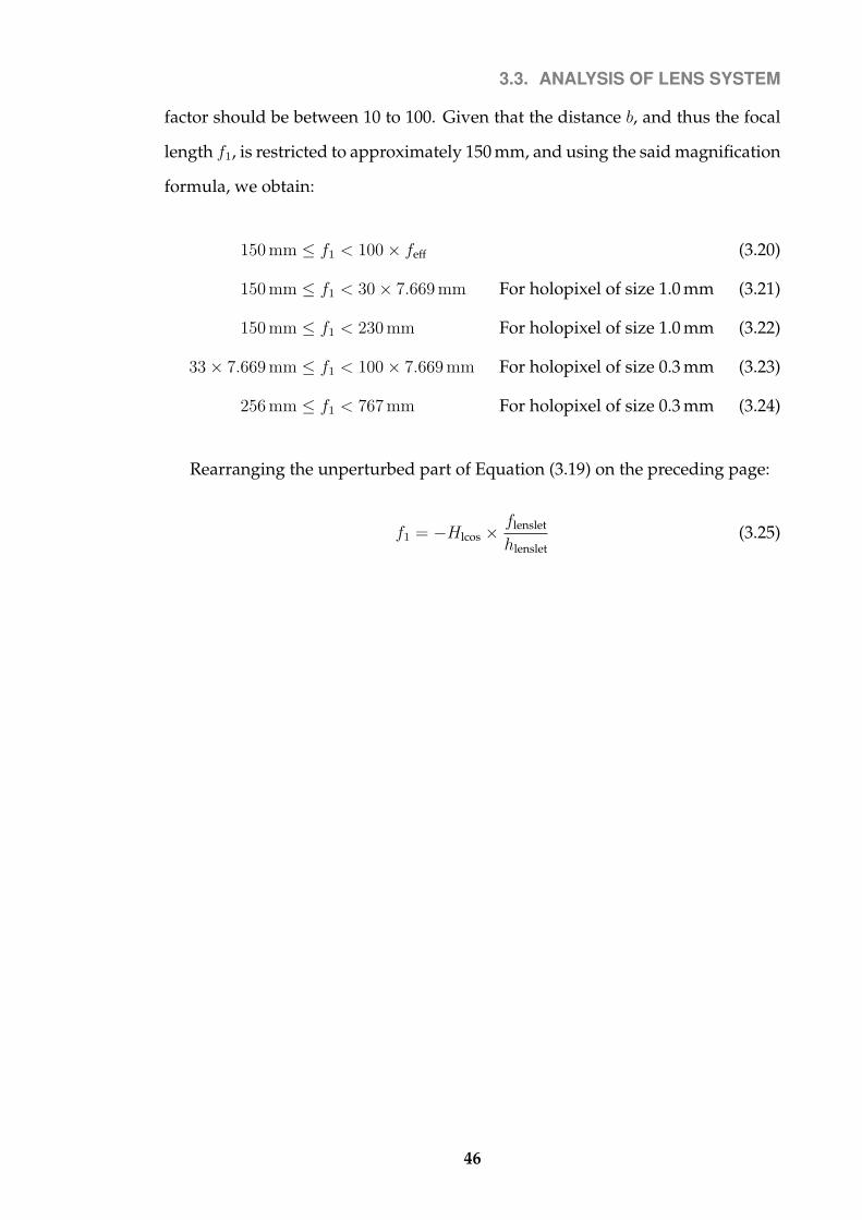
3.3. ANALYSIS OF LENS SYSTEM
factor should be between 10 to 100. Given that the distance b, and thus the focal
length f1, is restricted to approximately 150 mm, and using the said magnification
formula, we obtain:
150 mm ≤ f1 < 100× feff (3.20)
150 mm ≤ f1 < 30× 7.669 mm For holopixel of size 1.0 mm (3.21)
150 mm ≤ f1 < 230 mm For holopixel of size 1.0 mm (3.22)
33× 7.669 mm ≤ f1 < 100× 7.669 mm For holopixel of size 0.3 mm (3.23)
256 mm ≤ f1 < 767 mm For holopixel of size 0.3 mm (3.24)
Rearranging the unperturbed part of Equation (3.19) on the preceding page:
f1 = −Hlcos ×flenslet
hlenslet(3.25)
46

3.3. ANALYSIS OF LENS SYSTEM
3.3.6 Summary
Choose the required holopixel radius, r. Typically 1.0 mm ≥ 2r ≥ 0.3 mm.
For a given microlens array with lenslets with a height of hlenslet and a focal length
of flenslet, determine the required focal length of lens L1, f1.
f1 = −Hlcos ×flenslet
hlenslet(3.26)
Ensure that the chosen microlens array sets f1 within the range:
150 mm ≤ f1 < 230 mm For holopixel of size 1.0 mm (3.27)
256 mm ≤ f1 < 767 mm For holopixel of size 0.3 mm (3.28)
Place the lens L1 at a distance b ≈ f1, such that b is a few millimeters different
from f1, to slightly defocus the holopixel image. Place the microlens array at a
distance a from the lens L1 such the a = f1.
Use a square or circular aperture with a height y, placed against the microlens
array, where y is:
y = 2r · f1
feff(3.29)
47

3.3. ANALYSIS OF LENS SYSTEM
3.3.7 Example microlens array
The necessary formulas for determining the properties of the microlens array and
lenses were established in the previous section. The distance b (From L1 to the
LCOS, illustrated in Figure 3.5 on page 28) is restricted by the requirement that
the clear height of the diverging beam is set by the clear height of the interven-
ing beam splitter and mirror. The distance is further restricted by the physical
minimum spacing between the LCOS, beam splitter and mirror. This restricts the
minimum distance of b to approximately 150 mm (Figure 3.3 on page 24).
The display used in this printer is a reflective LCOS display made by the com-
pany Brillian. The model is the BR1080HC, and the dimensions are shown in
Figure 3.12 on the next page. The LCOS is used in landscape format.
This Brillian LCOS has a display screen height of 10.56 mm (See Figure 3.12
on the following page), requiring that the illuminating beam has a height equal
to this to ensure full illumination without unnecessary loss of energy. With this
requirement, Hlcos = 10.56 mm.
Applying the determined values to the unperturbed term in Equation (3.19)
on page 45, the desired ratio of lenslet height hlenslet to lenslet focal length flenslet
is obtained:
hlenslet
−flenslet≤ 10.56 mm
150 mm(3.30)
=⇒ hlenslet
−flenslet≤ 0.07 (3.31)
Consider an LCOS with lenslets with a clear height of hlenslet = 0.2 mm and
a focal length of flenslet = −3.0 mm. This satisfies the condition since 0.2 mm ÷
3.0 mm = 0.67.
48

3.3. ANALYSIS OF LENS SYSTEM
Figure 3.12: Dimensional schematic of the Brillian LCOS Display BR1080HChttp://www.brilliancorp.com/PDF/projection/BR1080HC_BR_D4.pdf
First Second Third
Lenslet dimensions: 0.40×0.46 mm 0.20×0.23 mm 0.040×0.046 mmSpherical radius: 1.3 mm 0.65 mm 0.13 mm
Required magnification: 26.4 52.8 264.0Focal length flenslet: -0.4 mm -0.8 mm -4.0 mm
Required f1: 10.56 mm 42.24 mm 324.92 mmAperture size (r=1.0 mm): 1.38 mm 5.51 mm 42.37 mmAperture size (r=0.3 mm): 0.41 mm 1.65 mm 12.71 mm
Table 3.1: Microlens array properties
49

3.3. ANALYSIS OF LENS SYSTEM
From Equation (3.26) on page 47:
f1 = −Hlcos ×flenslet
hlenslet(3.32)
= 10.56 mm× 3.0 mm
0.2 mm(3.33)
= 158 mm (3.34)
For a 1.0 mm pixel the aperture has a height y, from Equation (3.29) on page 47,
of:
y = 2r · f1
feff(3.35)
= 1.0 mm · 158 mm
7.669 mm(3.36)
= 20.7 mm (3.37)
To obtain a circular holopixel that is 1.0 mm in diameter, the aperture needs to
also be circular with a diameter y of 20.7 mm. This would utilize approximately
20.72
0.22 = 10712 lenslets - sufficient to provide smooth illumination.
Three different microlens arrays that satisfy the condition in Equation (3.31)
on page 48 are experimentally tested in the next section for a qualitative analysis.
The three microlens arrays examined are all composed of an array of rectangular
lenslets with a dimensional ratio equal to that of the LCOS. The relevant details
along with the required focal length of lens L1 and required aperture height cal-
culated by the methods given here, are given in Table 3.1 on the previous page.
50
3.4. EXPERIMENTAL EVALUATION OF LENS ARRAY SYSTEM
3.4 Experimental evaluation of lens array system
In analogue holography a hologram is made by illuminated a physical object
with coherent light. The microscopic roughness of the surface of the object cre-
ates speckle which can present a serious visual problem. The final hologram can
appear to ’twinkle’ or ’sparkle’ and the effective resolution of the hologram is
several times lower than the diffraction limit [51].
In digital holography using a computer display, the problem of speckle is al-
most removed. A dot matrix of ’holopixels’ is printed, each with their own in-
dependent speckle. On replay with a white-light source, the human eye does
not observe any sparkling effects. Speckle does pose other problems however.
The speckle affects the angular distribution of intensity for each holopixel, as de-
scribed below.
There is an additional possible problem – speckle on image at the Fourier
plane may also affect the diffraction efficiency as the light intensity is not evenly
distributed across emulsion, thus not fully utilizing all of the grains.
Section 3.3.5 on page 40 analytically considered the microlens array system to
determine the optimal distance based upon the lenslet size, aperture size, pixel
size, and distances. However this approach does not take into account the ef-
fect of speckle. The microlens array acts as an array of mutually coherent point
light-sources. These point sources expand and overlap, each illuminating the
microlens array, creating an averaged illumination that hides any defects in the
beam quality (due to dust particles etc). An unwanted side-effect however is that
the mutually coherent sources interfere with each other creating speckle.
The speckle pattern created on the LCOS results in an effectively reduced res-
olution of the LCOS display system, reducing the possible depth of field of the
hologram (both into the hologram plane, and out of the hologram plane). A se-
vere degree of speckle can result in holograms with low fidelity and contrast.
To reduce the effect of speckle, a simple method was required that introduced
51

3.4. EXPERIMENTAL EVALUATION OF LENS ARRAY SYSTEM
minimal complexity and cost into the design. A brief summary of existing meth-
ods is presented below, with its applicability to digital holography noted. As
the speckle is affected by the properties of the microlens array and the optics be-
tween the microlens array and the LCOS, the simplest method was to try differ-
ent microlens arrays and different positions to qualitatively minimize the effect
of speckle.
The structure of the speckle is examined, followed by a subjective assessment
of the overall image quality. The results are summarized, and the microlens ar-
ray with the larger lenslets (rectangular lenslets of dimensions 0.40 mm×0.46 mm
with a curvature of radius of 1.3 mm) was chosen for future digital holography
research.
The raw recorded data is presented in Appendix I.
3.4.1 Previous work
The problem of speckle due to a coherent source on a microlens array has been
tackled many times. Goodman [52] showed over 30 years ago that speckle can be
regarded as arising from a classical random walk in the complex plane. Reduc-
ing the contrast or smoothing the speckle requires diversity in the polarization,
space, frequency or time. In the proceeding years, each of these avenues were
investigated with varying success for use in many different fields in science. Iwai
and Asakura [53] summarize the 30 years of research into each of these differ-
ent avenues. The applicability of these approaches to digital holography is very
briefly given here.
For pulsed holography, time varying the polarization in a pulse would de-
stroy the diffraction gratings on the hologram. Compositing both horizontal and
vertical polarizations on to a single pixel may possibly work, although it would
present practical difficulties.
Increasing spatial diversity has been used with moderate success in analogue
52
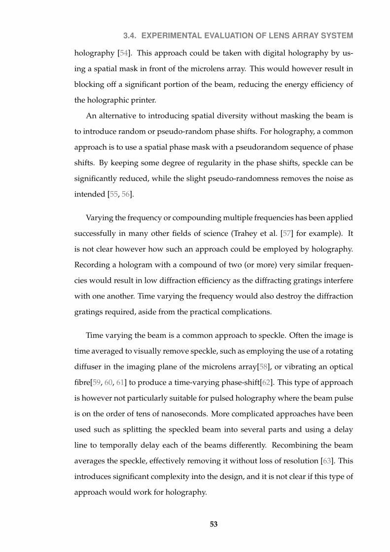
3.4. EXPERIMENTAL EVALUATION OF LENS ARRAY SYSTEM
holography [54]. This approach could be taken with digital holography by us-
ing a spatial mask in front of the microlens array. This would however result in
blocking off a significant portion of the beam, reducing the energy efficiency of
the holographic printer.
An alternative to introducing spatial diversity without masking the beam is
to introduce random or pseudo-random phase shifts. For holography, a common
approach is to use a spatial phase mask with a pseudorandom sequence of phase
shifts. By keeping some degree of regularity in the phase shifts, speckle can be
significantly reduced, while the slight pseudo-randomness removes the noise as
intended [55, 56].
Varying the frequency or compounding multiple frequencies has been applied
successfully in many other fields of science (Trahey et al. [57] for example). It
is not clear however how such an approach could be employed by holography.
Recording a hologram with a compound of two (or more) very similar frequen-
cies would result in low diffraction efficiency as the diffracting gratings interfere
with one another. Time varying the frequency would also destroy the diffraction
gratings required, aside from the practical complications.
Time varying the beam is a common approach to speckle. Often the image is
time averaged to visually remove speckle, such as employing the use of a rotating
diffuser in the imaging plane of the microlens array[58], or vibrating an optical
fibre[59, 60, 61] to produce a time-varying phase-shift[62]. This type of approach
is however not particularly suitable for pulsed holography where the beam pulse
is on the order of tens of nanoseconds. More complicated approaches have been
used such as splitting the speckled beam into several parts and using a delay
line to temporally delay each of the beams differently. Recombining the beam
averages the speckle, effectively removing it without loss of resolution [63]. This
introduces significant complexity into the design, and it is not clear if this type of
approach would work for holography.
53

3.4. EXPERIMENTAL EVALUATION OF LENS ARRAY SYSTEM
3.4.2 Experimental setup
The following microlens arrays were considered3:
1. Table I.1 on page 177 examines the first microlens array with each lenslet
being rectangular with physical dimensions of 0.40 mm×0.46 mm. These
lenslets are spherical lenses with a radius of 1.3 mm.
2. Table I.2 on page 179 examines the second microlens array with each lenslet
being rectangular with physical dimensions of 0.20 mm×0.23 mm. These
lenslets are spherical lenses with a radius of 0.65 mm.
3. Table I.3 on page 181 examines the third microlens array with each lenslet
being rectangular with physical dimensions of 0.040 mm×0.046 mm. These
lenslets are spherical lenses with a radius of 0.13 mm.
To test the three microlens array arrays, the lens system was setup as previ-
ously described in Section 3.3 on page 30. Each of the three different microlens
array arrays were tried at different positions. The pulsed laser was switched
producing a projected image from the final objective lens. When printing, the
photosensitive hologram plate would be placed a few millimeters away from the
objective lens, in the Fourier plane of the image of the LCOS display system. This
experiment instead removed any hologram plate, and projected the image of the
LCOS on to a white board 1.2 m from the lens objective.
The contrast and intensity of the speckle relative to the displayed image was
determined by the properties of microlens array array as well as its position. The
overall ’noise’ (intensity strength relative to the displayed image) of the speckle
was recorded, along with the size and shape of the beam profile where it illumi-
nates the LCOS display system.
The speckle in the projected image also containted a repeating pattern. The
size of these repeating patterns was measured by measuring the size of a multiple3A style note: For those with a colour version of this report, the data for the first microlens
array is always plotted and referenced in a blue color, the second microlens array uses purple/red,and the third microlens array uses green. This is purely a visual aid to the reader.
54

3.4. EXPERIMENTAL EVALUATION OF LENS ARRAY SYSTEM
number of these repeating structures with a ruler.
Appendix I gives the raw recorded data for the three different microlens array
arrays at different positions.
As an important experimental note: If the microlens array array focal point
is imaged directly onto the LCOS, the energy density on the LCOS can be suffi-
ciently high to risk breaking the LCOS. This was avoided and noted in the tables
were applicable.
3.4.3 Image quality
Figure 3.13 on the next page graphs the quality of the projected image of the LCOS
display based upon a subjective judgment of the quality of the image. A large
range of positions was tested, however the range is limited by the Equation (3.5)
on page 38; the microlens array is required to be positioned at approximately
the distance of the focal length of the lens that images it onto the LCOS display.
Figure 3.14 on page 57, Figure 3.15 on page 58 and Figure 3.16 on page 58 judge
a suitable range for the LCOS based upon intensity distribution across the LCOS
(A smooth, even distribution is required, as opposed to a Gaussian distribution
if the lens array is too close) and the shape of the beam (The whole of the LCOS
should be illuminated with little energy wasted).
55

3.4. EXPERIMENTAL EVALUATION OF LENS ARRAY SYSTEM
Image quality against lens array position
Very Good
Good
Fair
Mediocre
Poor
Very Poor
0.0 1.0 2.0 3.0 4.0 5.0 6.0 7.0 8.0 9.0 10.0 11.0 12.0 13.0 14.0
Lens array position / cm
Imag
e qu
ality
First lens array Second lens array Third lens array
Figure 3.13: The subjectively judged quality of the projected image of the LCOSon a white board 1.2 m away from the objective lens, due to speckle noise. Animage judged as Very Good would have a nearly unnoticeable amount of visualspeckle. The data is drawn from the recorded data in Appendix I.
56

3.4. EXPERIMENTAL EVALUATION OF LENS ARRAY SYSTEM
Image quality and intensity against lens array position (First lens array)
Very Good
Good
Fair
Mediocre
Poor
Very Poor 0.0 1.0 2.0 3.0 7.0 8.0 9.0 10.0 11.0 12.0 13.0 14.0
Lens array position / cm
Image Quality Intensity & Shape
5.0 6.0 4.0
Figure 3.14: The size and shape of the beam must be sufficiently close to thesize and shape of the LCOS. Additionally the illumination intensity across theLCOS must be spatially smooth and even. These two factors were consideredtogether, using the recorded data in Appendix I, and drawn here as the ‘Intensity& Shape’ curve. This is drawn with the Image Quality curve shown in Figure 3.13for comparison. This graph is shown for the first microlens array. A suitableregion for the distance between the microlens array and closest lens such thatthe image quality, beam intensity and beam shape are all at least acceptable isbetween approximately 4.0 cm to 6.0 cm.
57
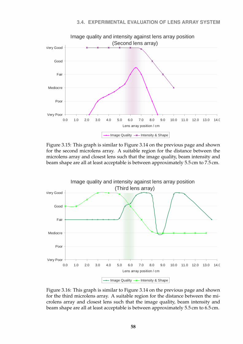
3.4. EXPERIMENTAL EVALUATION OF LENS ARRAY SYSTEM
Image quality and intensity against lens array position(Second lens array)
Very Poor
Poor
Mediocre
Fair
Good
Very Good
0.0 1.0 2.0 3.0 4.0 5.0 6.0 7.0 8.0 9.0 10.0 11.0 12.0 13.0 14.0 Lens array position / cm
Image Quality Intensity & Shape
Figure 3.15: This graph is similar to Figure 3.14 on the previous page and shownfor the second microlens array. A suitable region for the distance between themicrolens array and closest lens such that the image quality, beam intensity andbeam shape are all at least acceptable is between approximately 5.5 cm to 7.5 cm.
Image quality and intensity against lens array position(Third lens array)
Very Good
Good
Fair
Mediocre
Poor
Very Poor 0.0 1.0 2.0 3.0 4.0 5.0 6.0 7.0 8.0 9.0 10.0 11.0 12.0 13.0 14.0
Lens array position / cm
Image Quality Intensity & Shape
Figure 3.16: This graph is similar to Figure 3.14 on the previous page and shownfor the third microlens array. A suitable region for the distance between the mi-crolens array and closest lens such that the image quality, beam intensity andbeam shape are all at least acceptable is between approximately 5.5 cm to 6.5 cm.
58
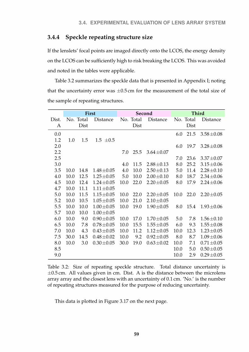
3.4. EXPERIMENTAL EVALUATION OF LENS ARRAY SYSTEM
3.4.4 Speckle repeating structure size
If the lenslets’ focal points are imaged directly onto the LCOS, the energy density
on the LCOS can be sufficiently high to risk breaking the LCOS. This was avoided
and noted in the tables were applicable.
Table 3.2 summarizes the speckle data that is presented in Appendix I; noting
that the uncertainty error was ±0.5 cm for the measurement of the total size of
the sample of repeating structures.
First Second ThirdDist.
ANo. Total
DistDistance No. Total
DistDistance No. Total
DistDistance
0.0 6.0 21.5 3.58±0.081.2 1.0 1.5 1.5 ±0.52.0 6.0 19.7 3.28±0.082.2 7.0 25.5 3.64±0.072.5 7.0 23.6 3.37±0.073.0 4.0 11.5 2.88±0.13 8.0 25.2 3.15±0.063.5 10.0 14.8 1.48±0.05 4.0 10.0 2.50±0.13 5.0 11.4 2.28±0.104.0 10.0 12.5 1.25±0.05 5.0 10.0 2.00±0.10 8.0 18.7 2.34±0.064.5 10.0 12.4 1.24±0.05 10.0 22.0 2.20±0.05 8.0 17.9 2.24±0.064.7 10.0 11.1 1.11±0.055.0 10.0 11.5 1.15±0.05 10.0 22.0 2.20±0.05 10.0 22.0 2.20±0.055.2 10.0 10.5 1.05±0.05 10.0 21.0 2.10±0.055.5 10.0 10.0 1.00±0.05 10.0 19.0 1.90±0.05 8.0 15.4 1.93±0.065.7 10.0 10.0 1.00±0.056.0 10.0 9.0 0.90±0.05 10.0 17.0 1.70±0.05 5.0 7.8 1.56±0.106.5 10.0 7.8 0.78±0.05 10.0 15.5 1.55±0.05 6.0 9.3 1.55±0.087.0 10.0 4.3 0.43±0.05 10.0 11.2 1.12±0.05 10.0 12.3 1.23±0.057.5 30.0 14.5 0.48±0.02 10.0 9.2 0.92±0.05 8.0 8.7 1.09±0.068.0 10.0 3.0 0.30±0.05 30.0 19.0 0.63±0.02 10.0 7.1 0.71±0.058.5 10.0 5.0 0.50±0.059.0 10.0 2.9 0.29±0.05
Table 3.2: Size of repeating speckle structure. Total distance uncertainty is±0.5 cm. All values given in cm. Dist. A is the distance between the microlensarray array and the closest lens with an uncertainty of 0.1 cm. ’No.’ is the numberof repeating structures measured for the purpose of reducing uncertainty.
This data is plotted in Figure 3.17 on the next page.
59

3.4. EXPERIMENTAL EVALUATION OF LENS ARRAY SYSTEM
Speckle pattern size against lens array position
0
0.5
1
1.5
2
2.5
3
3.5
4
0.0 1.0 2.0 3.0 4.0 5.0 6.0 7.0 8.0 9.0
Lens array position / cm
Spe
ckle
pat
tern
siz
e / c
m
First lens array Second lens array Third lens array
Figure 3.17: Repeating speckle structure size plotting against position of mi-crolens array for each of the three different microlens arrays.
The size of the speckle patterns is smallest for the first microlens array, which
is the microlens array with the largest lenslets and with the largest radius of cur-
vature. It is not entirely clear how much effect this structure will have on the final
hologram.
60

3.4. EXPERIMENTAL EVALUATION OF LENS ARRAY SYSTEM
3.4.5 Microlens array focal plane
There is another concern regarding the position of the microlens array. The plane
of the aperture that is imaged on to the photosensitive emulsion is very close to
the microlens array. As the lenslets have a small focal distance, the aperture is also
very close to the virtual image of the focal plane of the microlens array. It is my
concern that if the imaged focal plane of the microlens array coincides with the
plane of the photosensitive emulsion, this will result in an uneven illumination
of the film, significantly reducing diffraction efficiency.
To monitor this effect, the data in Appendix I records the relative distance
of the lenslet focal plane from the hologram plate. This distance could not be
measured directly, so to measure this a piece of white card was placed inside the
afocal telescopic lens system and moved into position such that the focal point of
the microlens array was focused onto the card. This could be seen clearly as an
array of points of light. The distance between this position and the image plane
of the aperture was recorded. All the distances given below are in terms of the
distance measured between the imaged focal plane of the microlens array and
the corresponding imaged plane of the aperture in telescopic lens system. The
position of the aperture remained unmoved and the only variable changed was
the position of the microlens array. It is worth noting that moving the microlens
array will in turn slightly move the plane that the aperture is focused on near the
hologram plane.
Extracting this distance data from the tables for the first, second and third
microlens arrays we get Table 3.3 on the following page.
61

3.4. EXPERIMENTAL EVALUATION OF LENS ARRAY SYSTEM
Microlensarray
First Second Third
dist. (cm) (cm) (cm) (cm)
0.0 12.51.2 8.02.0 10.02.2 10.52.5 9.53.0 8.0 8.53.5 5.5 8.0 8.04.0 4.2 7.4 7.54.5 4.0 6.4 5.54.7 2.15.0 1.5 5.0 2.15.2 0.05.5 -0.8 2.0 0.25.7 -1.76.0 -4.0 0.0 -1.86.5 -6.8 -3.5 -5.07.0 -19.0 -10.0 -9.87.5 -17.0 -15.08.0 -17.0
Table 3.3: Distance measured between the imaged focal plane of the microlens ar-ray and the corresponding imaged plane of the aperture in telescopic lens system.All values given with uncertainty of ±0.5 cm.
62
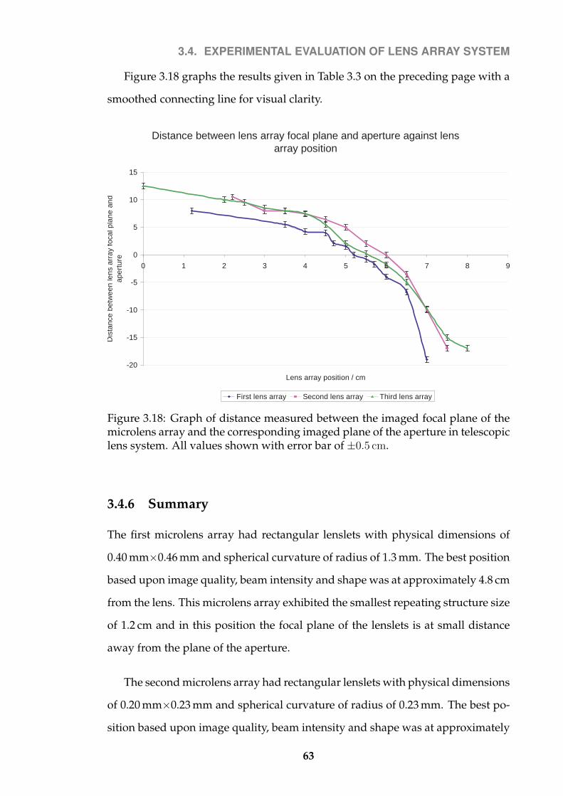
3.4. EXPERIMENTAL EVALUATION OF LENS ARRAY SYSTEM
Figure 3.18 graphs the results given in Table 3.3 on the preceding page with a
smoothed connecting line for visual clarity.
Distance between lens array focal plane and aperture against lens array position
-20
-15
-10
-5
0
5
10
15
0 1 2 3 4 5 6 7 8 9
Lens array position / cm
Dis
tanc
e be
twee
n le
ns a
rray
foca
l pla
ne a
nd
aper
ture
First lens array Second lens array Third lens array
Figure 3.18: Graph of distance measured between the imaged focal plane of themicrolens array and the corresponding imaged plane of the aperture in telescopiclens system. All values shown with error bar of ±0.5 cm.
3.4.6 Summary
The first microlens array had rectangular lenslets with physical dimensions of
0.40 mm×0.46 mm and spherical curvature of radius of 1.3 mm. The best position
based upon image quality, beam intensity and shape was at approximately 4.8 cm
from the lens. This microlens array exhibited the smallest repeating structure size
of 1.2 cm and in this position the focal plane of the lenslets is at small distance
away from the plane of the aperture.
The second microlens array had rectangular lenslets with physical dimensions
of 0.20 mm×0.23 mm and spherical curvature of radius of 0.23 mm. The best po-
sition based upon image quality, beam intensity and shape was at approximately
63

3.4. EXPERIMENTAL EVALUATION OF LENS ARRAY SYSTEM
6.7 cm from the lens. At this position, the repeating structure size is approxi-
mately 1.4 cm, and the focal plane of the lenslets is at a distance away from the
plane of the aperture.
The third microlens array had rectangular lenslets with physical dimensions
of 0.040 mm×0.046 mm and spherical curvature of radius of 0.13 mm. The best
position based upon image quality, beam intensity and shape was at approxi-
mately 6.0 cm from the lens. At this position, the repeating structure size is the
largest of the three lens arrays at approximately 1.6 cm. The focal plane of the
lenslets is close to the plane of the aperture.
There does not appear to be any significant differences between using the
three microlens arrays. They each exhibited quite different behavior, but when
all of the factors are taken into account, there is no clear superior choice.
For future work, the first microlens array was chosen due to the smaller re-
peating speckle structure.
64
3.5. MINIMIZING BEAM ENERGY LOSS IN LENS SYSTEM
3.5 Minimizing beam energy loss in lens system
The Red Green Blue (RGB) digital hologram printer design by Ratcliffe et al. [47]
utilizes a long cavity Nd:YAG laser to provide sufficient energy to illuminate the
silver halide emulsion. The energy required from the laser, per color channel, is
dependant upon the size of the printed holopixel, the efficiency of the hologram
printer (lens system, display system) and the sensitivity of the photo-sensitive
emulsion to the illumination wavelength and pulse length used.
For the printing of monochromatic green holograms, a green-sensitive mono-
chromatic fine-grain emulsion such as VRP-M (Zacharovas et al. [see 64]) from
Slavich [65] is sufficient. This particular emulsion is sensitive to pulse lengths
from nanosecond pulses up to CW laser emission. For pulsed radiation with a
length of around tens of nanoseconds, the VRP-M emulsion requires an energy
density of approximately 60 J/cm2 for maximum diffraction efficiency4.
For the production of true color volume holograms, a panchromatic or dichro-
matic gelatine emulsion is required, such as the ultra-fine grain emulsion known
as PFG-03C [64] from Slavich [65] 5. The fine size of the grains makes the emulsion
less sensitive to radiation, requiring an energy density approximately 3.0 mJ/cm2
of green-light pulsed radiation6 for maximum diffraction efficiency. Some charac-
teristics of the Slavich color emulsion have been presented by Markov [66], with
a further more theoretical analysis on selective characteristics of single layer color
holograms by Markov and Khizhnyak [67]. An overview of the current state of
colour reflection holography is given by Bjelkhagen et al. [68].
Ratcliffe et al. [47] proposes the use of a long cavity Nd:YAG pulsed laser,
produced by Geola Technologies, which has a repetition rate of up to ten pulses
per second and can provide ample energy for such a system (Typically around
4http://www.geola.com/45.asp5A photographic company outside Moscow. See References.6http://www.geola.com/48.asp
65

3.5. MINIMIZING BEAM ENERGY LOSS IN LENS SYSTEM
15 mJ for the second harmonic). In this context, the energy efficiency of the system
is not of high importance.
There are however many advantages to minimizing energy loss. Increasing
the laser repetition rate is technologically simpler if the energy in each shot is
decreased. Likewise if a short cavity laser is utilized instead of a long cavity
laser, a more stable output is achieved at the sacrifice of shot energy. The use of a
short cavity laser also offers a simpler design, making the system cheaper due to
less components required and a shorter build and maintenance period of time.
The biggest loss of energy in the system by Ratcliffe et al. [47] is in the LCD
display system. The system detailed in the section utilizes an LCOS system to
increase the efficiency by approximately 30 percentile points, and a series of mag-
nifying relay lenses to minimize energy loss at the apertures.
An extra system of magnifying relay lenses can be used to reduce the energy
loss on the apertures on both the reference and object beams by reducing the beam
size to the size of the apertures. Such a system of magnifying relay lenses is also
useful to control the size of the object beam at the plane of the microlens array.
The spatial profile of the beam at the microlens array is geometrically similar to
the spatial profile of the beam on the hologram plate. To clean the reference beam,
a small aperture was placed at the mutual focal point of the magnifying relay
lenses and adjusted with the aid of a laser beam spatial profiler placed upstream.
66

3.6. SUMMARY
3.6 Summary
A digital hologram printer was developed and built based upon the design by
Ratcliffe et al. [47]. The steps required reproduce the creation of a hologram
printer are given, mixed in with lessons learned from the accumulated expe-
rience of building and maintaining three such printers. A new display system
(LCOS display) was investigated and found to have a significant advantage over
the LCD display system used by Ratcliffe et al. [47]. The lens systems were analyt-
ically examined by various approximations and methods to determine a simple
set of formulas to allow the holopixel spatial size to be easily adjusted by the
hologram printer operator.
Three microlens arrays were qualitatively analyzed by a series of experiments
and they were found to perform almost equally well, demonstrating that the
properties of the microlens array do not have a significant effect on the hologram
quality, within the parameter space tested.
A brief mention on increasing the energy efficiency of the design was made,
with the goal of replacing the long cavity laser with a short cavity laser. A short
cavity laser would have the advantage of increasing the laser energy point-to-
point stability while also lowering the overall cost. Minimizing energy loss is
discussed further in Chapter 5.
Figure 3.19 on the next page demonstrates the working hologram printer.
67

3.6. SUMMARY
Figure 3.19: Photograph of green dragon hologram with 1 mm×1 mm pixelsprinted on the described hologram printer. Note that there are occasionalincorrectly-dim pixels due to the laser energy instabilities. This is discussed andfixed in Chapter 6 on page 113.
68

4White logo
This chapter looks at a common problem with printing digital holograms that
have a large contrast range. A specific hologram is studied to study this prob-
lematic ’ghosting’ effect and the cause is identified. A set of Matlab programs are
written to test possible solutions and their effectiveness is determined.
4.1 Overview
Figure 4.2a on page 74 is a photograph of a white-light-viewable full-color holo-
gram that was printed on a RGB hologram printer that is similar in design to
that described in this thesis. In particular, the same Brillian LCOS display system
was utilized, along with the same lens systems. The photograph was taken at an
angle normal to the hologram. The intended result was to produce a hologram
that looks similar to the rendered image for that angle, as shown in Figure 4.2c
on page 74.
69
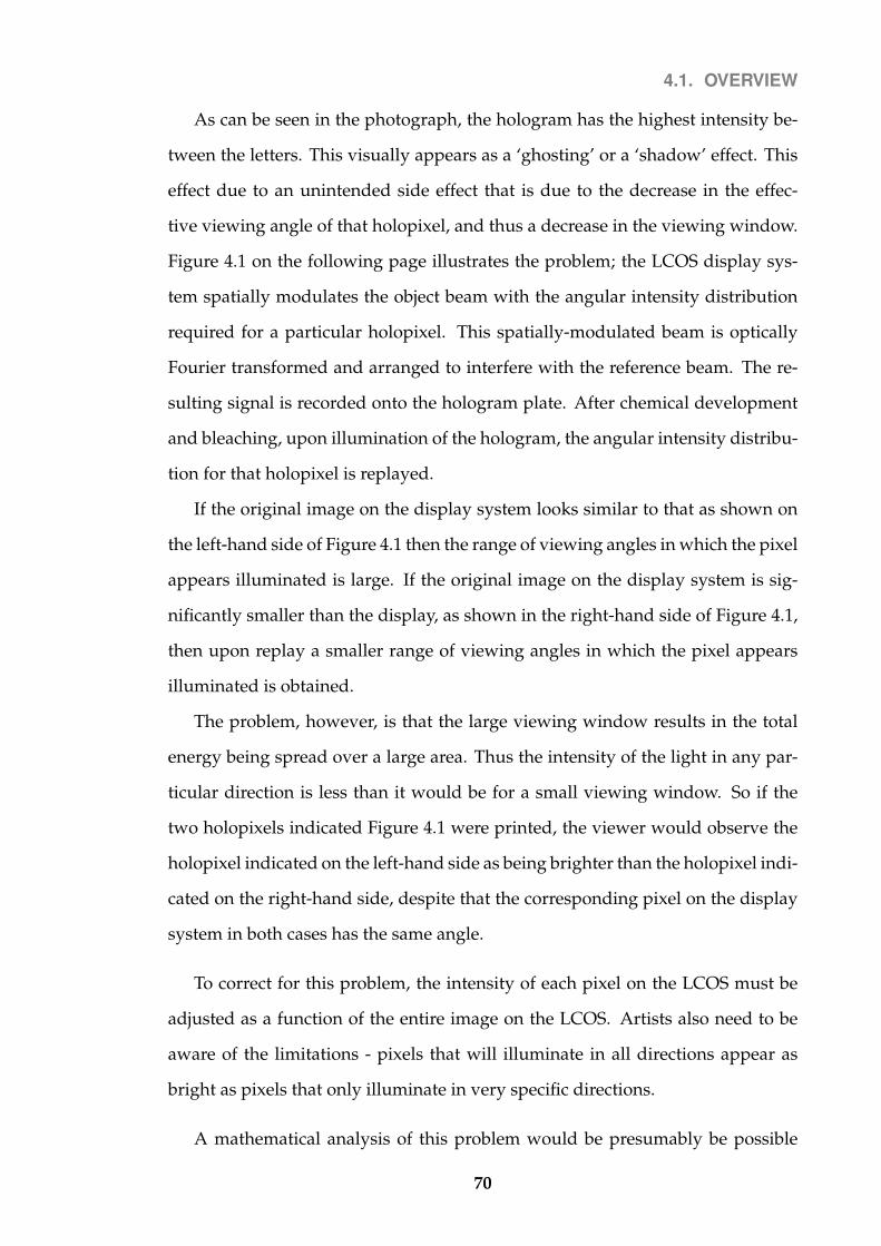
4.1. OVERVIEW
As can be seen in the photograph, the hologram has the highest intensity be-
tween the letters. This visually appears as a ‘ghosting’ or a ‘shadow’ effect. This
effect due to an unintended side effect that is due to the decrease in the effec-
tive viewing angle of that holopixel, and thus a decrease in the viewing window.
Figure 4.1 on the following page illustrates the problem; the LCOS display sys-
tem spatially modulates the object beam with the angular intensity distribution
required for a particular holopixel. This spatially-modulated beam is optically
Fourier transformed and arranged to interfere with the reference beam. The re-
sulting signal is recorded onto the hologram plate. After chemical development
and bleaching, upon illumination of the hologram, the angular intensity distribu-
tion for that holopixel is replayed.
If the original image on the display system looks similar to that as shown on
the left-hand side of Figure 4.1 then the range of viewing angles in which the pixel
appears illuminated is large. If the original image on the display system is sig-
nificantly smaller than the display, as shown in the right-hand side of Figure 4.1,
then upon replay a smaller range of viewing angles in which the pixel appears
illuminated is obtained.
The problem, however, is that the large viewing window results in the total
energy being spread over a large area. Thus the intensity of the light in any par-
ticular direction is less than it would be for a small viewing window. So if the
two holopixels indicated Figure 4.1 were printed, the viewer would observe the
holopixel indicated on the left-hand side as being brighter than the holopixel indi-
cated on the right-hand side, despite that the corresponding pixel on the display
system in both cases has the same angle.
To correct for this problem, the intensity of each pixel on the LCOS must be
adjusted as a function of the entire image on the LCOS. Artists also need to be
aware of the limitations - pixels that will illuminate in all directions appear as
bright as pixels that only illuminate in very specific directions.
A mathematical analysis of this problem would be presumably be possible
70

4.1. OVERVIEW
xlcos
ylcos
LCOSxlcos
ylcos
LCOS
xhologram
yhologram
z
eye
xhologram
yhologram
z
eye
viewing window
Figure 4.1: The Fourier transform of the image on the LCOS is printed on tothe hologram as a single ’holopixel’. Upon replay of the hologram, this recordedFourier image is reconstructed as an angular intensity distribution. If the viewingwindow is smaller, as shown on the right, then the overall intensity as seen by theeye will be larger.
71
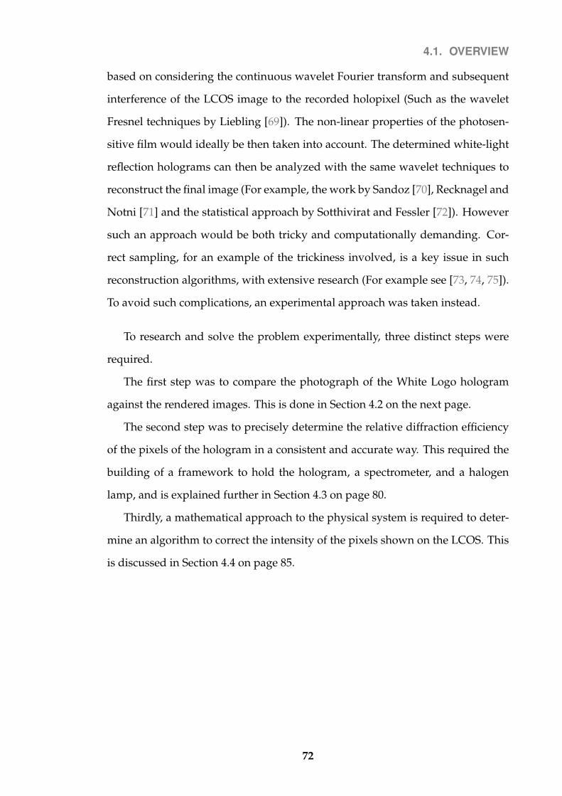
4.1. OVERVIEW
based on considering the continuous wavelet Fourier transform and subsequent
interference of the LCOS image to the recorded holopixel (Such as the wavelet
Fresnel techniques by Liebling [69]). The non-linear properties of the photosen-
sitive film would ideally be then taken into account. The determined white-light
reflection holograms can then be analyzed with the same wavelet techniques to
reconstruct the final image (For example, the work by Sandoz [70], Recknagel and
Notni [71] and the statistical approach by Sotthivirat and Fessler [72]). However
such an approach would be both tricky and computationally demanding. Cor-
rect sampling, for an example of the trickiness involved, is a key issue in such
reconstruction algorithms, with extensive research (For example see [73, 74, 75]).
To avoid such complications, an experimental approach was taken instead.
To research and solve the problem experimentally, three distinct steps were
required.
The first step was to compare the photograph of the White Logo hologram
against the rendered images. This is done in Section 4.2 on the next page.
The second step was to precisely determine the relative diffraction efficiency
of the pixels of the hologram in a consistent and accurate way. This required the
building of a framework to hold the hologram, a spectrometer, and a halogen
lamp, and is explained further in Section 4.3 on page 80.
Thirdly, a mathematical approach to the physical system is required to deter-
mine an algorithm to correct the intensity of the pixels shown on the LCOS. This
is discussed in Section 4.4 on page 85.
72

4.2. PHOTOGRAPH ANALYSIS
4.2 Photograph analysis
To better understand the problem, the photograph of the White Logo hologram
(Figure 4.2a on the following page) was analyzed against the series of rendered
images that were used to create the said hologram.
To compare the photograph and the rendered images programmatically, the
photograph and images were carefully cropped and scaled such that the photo-
graph could be matched pixel-wise with the image. This was done by the follow-
ing Linux command that utilizes the ImageMagick convert program:
for f in white_0*.png; do
convert $f -crop "295x108+97+115" \
-geometry 557x205! ../WhiteLogoPngMine/$f
done
Where the parameters were found through a trial-and-error effort.
73
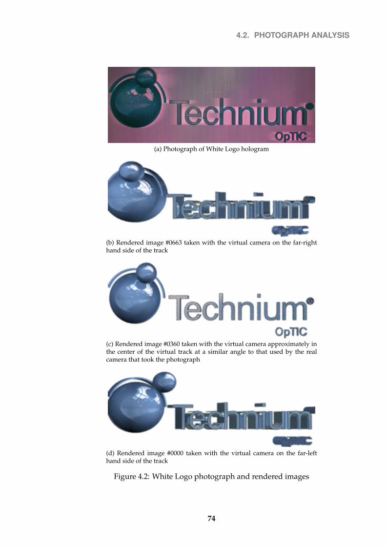
4.2. PHOTOGRAPH ANALYSIS
(a) Photograph of White Logo hologram
(b) Rendered image #0663 taken with the virtual camera on the far-righthand side of the track
(c) Rendered image #0360 taken with the virtual camera approximately inthe center of the virtual track at a similar angle to that used by the realcamera that took the photograph
(d) Rendered image #0000 taken with the virtual camera on the far-lefthand side of the track
Figure 4.2: White Logo photograph and rendered images
74

4.2. PHOTOGRAPH ANALYSIS
Appendix D gives the program listing for the code used to analyze the differ-
ence between the photograph and the rendered images. The results are shown
in Figure 4.3. There is a strong correlation for the low intensity pixels (the black
areas of the image) and a much weaker correlation for the high intensity pixels.
Figure 4.3: A plot of the intensity of each pixel on the photograph of the WhiteLogo hologram plotted against the corresponding pixel on the rendered imageshown in Figure 4.2c on the previous page. The intensity scale is arbitrarily be-tween 0 and 1 where 1 is a brighter, and 0 is darker. The images were convertedto greyscale and a Gaussian blur of 2 pixels in the horizontal direction appliedfirst.
It is the difference in intensities between the photograph (actual intensity) and
the center rendered image (intended intensity) that we are interested in, as it is
this difference that we need to compensate for. This difference is a function, f , of
the corresponding pixel on all of the rendered images. Indicating the photograph
intensity at a point (x,y) as P (x, y), the intensity of the center rendered image as
75
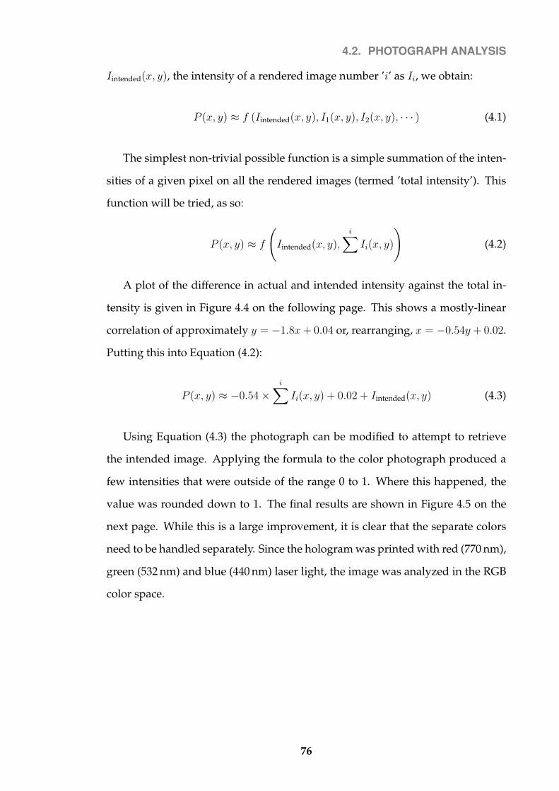
4.2. PHOTOGRAPH ANALYSIS
Iintended(x, y), the intensity of a rendered image number ’i’ as Ii, we obtain:
P (x, y) ≈ f (Iintended(x, y), I1(x, y), I2(x, y), · · · ) (4.1)
The simplest non-trivial possible function is a simple summation of the inten-
sities of a given pixel on all the rendered images (termed ’total intensity’). This
function will be tried, as so:
P (x, y) ≈ f
(Iintended(x, y),
i∑Ii(x, y)
)(4.2)
A plot of the difference in actual and intended intensity against the total in-
tensity is given in Figure 4.4 on the following page. This shows a mostly-linear
correlation of approximately y = −1.8x+ 0.04 or, rearranging, x = −0.54y + 0.02.
Putting this into Equation (4.2):
P (x, y) ≈ −0.54×i∑Ii(x, y) + 0.02 + Iintended(x, y) (4.3)
Using Equation (4.3) the photograph can be modified to attempt to retrieve
the intended image. Applying the formula to the color photograph produced a
few intensities that were outside of the range 0 to 1. Where this happened, the
value was rounded down to 1. The final results are shown in Figure 4.5 on the
next page. While this is a large improvement, it is clear that the separate colors
need to be handled separately. Since the hologram was printed with red (770 nm),
green (532 nm) and blue (440 nm) laser light, the image was analyzed in the RGB
color space.
76

4.2. PHOTOGRAPH ANALYSIS
Figure 4.4: A plot of the intensity of each pixel on the photograph minus theintensity of the corresponding pixel on the center rendered image of the WhiteLogo hologram, plotted against the corresponding total intensity of that pixel.The total intensity is a summation of the intensities of the given pixel for all ofthe rendered images. The intensity scale is arbitrarily between 0 and 1 where1 is a brighter, and 0 is darker. The images were converted to greyscale and aGaussian blur of 2 pixels in the horizontal direction applied first.
Figure 4.5: The photograph shown in Figure 4.2a on page 74 with Equation (4.3)on the previous page applied to each pixel
77

4.2. PHOTOGRAPH ANALYSIS
To attempt to produce better results, each channel was processed separately
in the RGB color space, and the results are shown in Figure 4.7 on the following
page.
The graph of the red channel, Figure 4.7a, has the least correlation, but at-
tempting a correlation anyway we get a linear correlation of approximately y =
−1.5x+ 0.2 or, rearranging, x = −0.67y + 0.08.
The green channel, Figure 4.7b, has better correlation but strongly appears to
be non-linear. Attempting a linear correlation anyway, we get a correlation of
approximately y = −2.0x, or x = −0.51y.
Finally, the blue channel, Figure 4.7c, has a strong linear correlation of approx-
imately y = −2.8x− 0.2, or x = −0.36y − 0.07.
Using these corrections with Equation (4.2) on page 76 but applying the cor-
rection separately to each channel, Figure 4.6 is obtained.
Figure 4.6: The photograph shown in Figure 4.2a on page 74 with the correctionapplied to each pixel. Each color channel was corrected separately, in RGB colorspace.
This is subjectively better, but not entirely satisfactory. It is still clearly brighter
in between the letters. Further work would be required on this.
To get a better analysis of the hologram, a spectrometer was used instead of
a photograph. This required a framework to support the spectrometer. This is
discussed in the next section.
78

4.2. PHOTOGRAPH ANALYSIS
(a) Red channel
(b) Green channel
(c) Blue channel
Figure 4.7: A plot of the intensity of each pixel on the photograph minus theintensity of the corresponding pixel on the center rendered image of the WhiteLogo hologram, plotted against the corresponding total intensity of that pixel.Each color channel has been plotted separately.
79
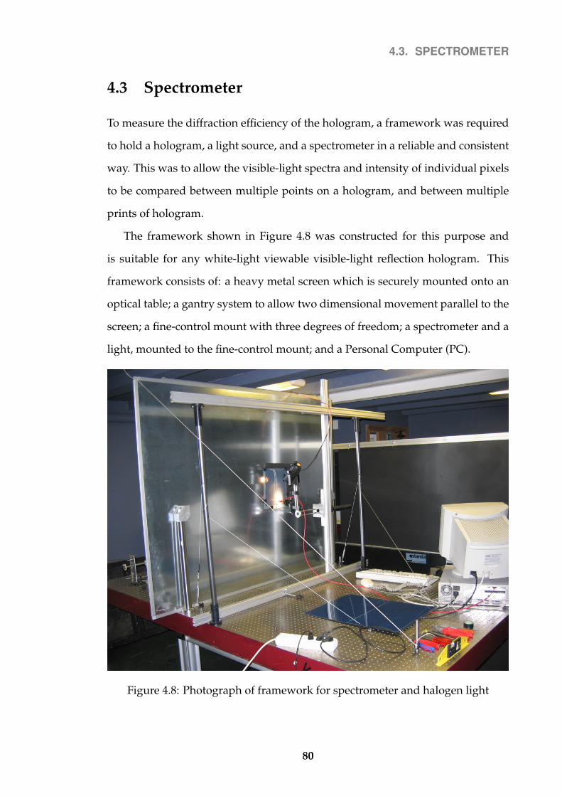
4.3. SPECTROMETER
4.3 Spectrometer
To measure the diffraction efficiency of the hologram, a framework was required
to hold a hologram, a light source, and a spectrometer in a reliable and consistent
way. This was to allow the visible-light spectra and intensity of individual pixels
to be compared between multiple points on a hologram, and between multiple
prints of hologram.
The framework shown in Figure 4.8 was constructed for this purpose and
is suitable for any white-light viewable visible-light reflection hologram. This
framework consists of: a heavy metal screen which is securely mounted onto an
optical table; a gantry system to allow two dimensional movement parallel to the
screen; a fine-control mount with three degrees of freedom; a spectrometer and a
light, mounted to the fine-control mount; and a Personal Computer (PC).
Figure 4.8: Photograph of framework for spectrometer and halogen light
80

4.3. SPECTROMETER
The metal screen can hold a hologram of up to 1.5 m×1.5 m in size and is
magnetic, allowing fragile holograms to be held in place with magnets. The main
2D gantry system was greased for easy movement and can be locked in place with
thumb-screws, to prevent accidental movement. The fine-control mount allows
the 60W halogen light to be held at almost any angle and height relative to the
spectrometer, and allows movement both parallel and normal to the screen. This
can also be locked into place to prevent accidental movement. The angle of the
halogen was set to the designed replay-angle for the holograms – equal to the
reference beam angle, 37◦ to the normal of the hologram, as shown in Figure 4.9.
Figure 4.9: Photograph of fine-control spectrometer mount
81

4.3. SPECTROMETER
The details of the spectrometer are given in Table 4.1. The spectrometer was
connected to a PC running OOIBase for Windows and SpectraWin, and was cali-
brated against a sheet of glossy white paper. Figure 4.10 shows the framework in
use on a white-light reflection hologram.
Figure 4.10: Photograph of spectrometer in use
Company: Ocean Optics EuropeModel: PC2000-ISADescription: PC Plug-in Fiber Optic SpectrometerGrating: 600 lines blazed at 500 nmBankwidth: 350-1000 nmOptions Installed: 25 µm SlitSerial: PC2E637Sample time: from 3 ms to 60 s
Table 4.1: Technical details of spectrometer
82

4.3. SPECTROMETER
Using the spectrometer framework on the White Logo hologram, the results
shown in Table 4.2 were obtained.
Position Red Channel Green ChannelWavelength Intensity Wavelength Intensity
White Region 625 33 505 28In between the ’n’ 627 145 508 106Next to top of H 628 120 509 85Next to the dot in ’i’ 628 131 508 94Next to floating sphere 629 181 509 150In the middle of the ’c’ 628 110 509 73In the middle top of ’c’ 629 194 509 133
Table 4.2: Wavelength and counts per minute for peak counts per minute in redand green channel. Wavelength is in nanometers, and intensity in counts perminute, as measured by the spectrometer detailed in Table 4.1 on the previouspage.
To test the accuracy the photograph of the White Logo hologram (Figure 4.2a
on page 74), the equivalent pixels in the photograph were compared against the
intensity recorded by the spectrometer. Table 4.3 shows the RGB values for the
equivalent pixels in the photograph, and Figure 4.11 on the following page is a
graph of the two sets of results plotted against each other, for each pixel and for
each channel.
Position Red Channel Green Channel Blue Channel
White Region 130 114 125In between the ’n’ 208 135 164Next to top of H 179 133 150Next to the dot in ’i’ 174 118 149Next to floating sphere 178 129 151In the middle of the ’c’ 171 124 149In the middle top of ’c’ 211 151 171
Table 4.3: Photograph intensity for the same position and angle as used by Ta-ble 4.2. The values have the range 0 to 255, with 255 being the maximum inten-sity.
83

4.3. SPECTROMETER
Spectrometer readings against pixel intensties on photograph for White Logo hologram
y = 0.4x + 121.8R2 = 0.7
y = 0.2x + 109.5R2 = 0.5
0
50
100
150
200
250
0 20 40 60 80 100 120 140 160 180 200
Spectrometer reading
Pho
togr
aph
pixe
l val
ue
Red Channel Green Channel Linear (Red Channel) Linear (Green Channel)
Figure 4.11: Spectrometer readings (From Table 4.2 on the previous page) plottedagainst the intensity value recorded by the camera for the same position and sameangle (From Table 4.3 on the preceding page). A linear-regression best-fit line isshown for the two color channels. The blue channel was not measured.
Figure 4.11 shows that the results from the camera do not match to sufficient
precision to the results from the spectrometer. This could be due to experimental
error, or an indication that the chosen camera was not of sufficiently quality to
capture a true-image of the scene. If the image from the camera was not an accu-
rate depiction of the light from the hologram, then this may explain some of the
noise in the results found in Section 4.2 on page 73.
84
4.4. FUTURE WORK
4.4 Future work
A more accurate correction algorithm that could remove most of the ghosting
problems would be a useful future work. This work could be based on a theoret-
ical approach to the problem, using coupled-wave theory to determine the exact
correction algorithm required. This algorithm can then be applied to the rendered
images so that the final printed hologram appears without any ghosting effects.
To provide a better avenue for investigation, a hologram was printed such
that the width of the viewing window is decreased for each holopixel, from left
to right. This was achieved by displaying a solid green rectangle of decreasing
width on the LCOS display. The results are given in Figure 4.12 on the next page.
The twelve lines were all printed the same, to allow for a more accurate analysis.
It is clear that the larger viewing window (to the left hand side of the pho-
tograph) results in a dimmer image in the direction normal to the hologram. It
would be useful future work to use the photographs to better analyze, and cor-
rect for, this problem. To further help with the problem, several holograms were
also printed with the object beam energy decreasing in steps. This was achieved
by changing the intensity of the rectangle display on the LCOS after every five
rows. Figure 4.13 on page 87 shows a photograph of a such a hologram. It is left
as future work to analyze these.
85
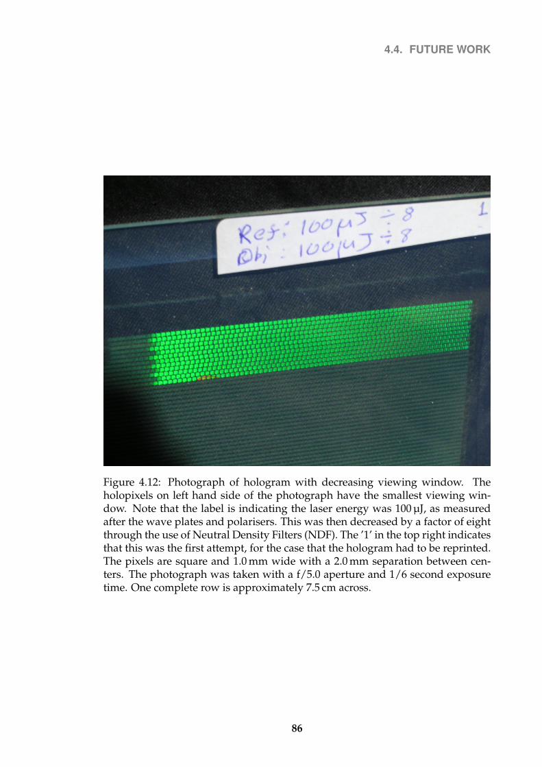
4.4. FUTURE WORK
Figure 4.12: Photograph of hologram with decreasing viewing window. Theholopixels on left hand side of the photograph have the smallest viewing win-dow. Note that the label is indicating the laser energy was 100 µJ, as measuredafter the wave plates and polarisers. This was then decreased by a factor of eightthrough the use of Neutral Density Filters (NDF). The ’1’ in the top right indicatesthat this was the first attempt, for the case that the hologram had to be reprinted.The pixels are square and 1.0 mm wide with a 2.0 mm separation between cen-ters. The photograph was taken with a f/5.0 aperture and 1/6 second exposuretime. One complete row is approximately 7.5 cm across.
86
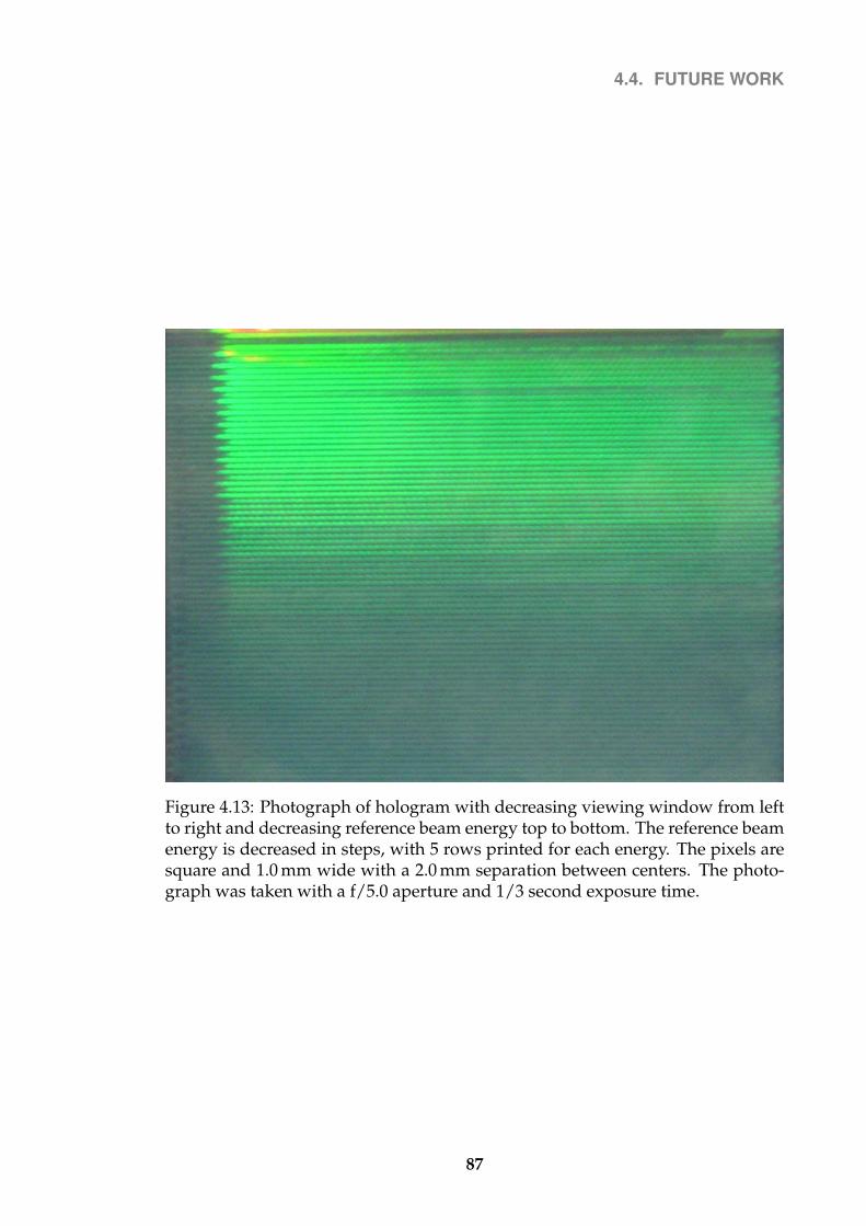
4.4. FUTURE WORK
Figure 4.13: Photograph of hologram with decreasing viewing window from leftto right and decreasing reference beam energy top to bottom. The reference beamenergy is decreased in steps, with 5 rows printed for each energy. The pixels aresquare and 1.0 mm wide with a 2.0 mm separation between centers. The photo-graph was taken with a f/5.0 aperture and 1/3 second exposure time.
87

4.5. SUMMARY
4.5 Summary
A sample hologram was found to have visual ‘shadows’ or ‘ghosting’ where the
size of the viewing window of a holopixel was determined to be affecting the ap-
parent brightness of the holopixel in any given direction. A photograph of the
hologram was compared to the set of rendered images and the intended image,
and correction algorithms were proposed. The correction algorithms were ap-
plied to the photograph and found to improve the image. These algorithms can
be applied to rendered images before printing to correct for ghosting.
The algorithms can also be used to inform the artists where ghosting would
occur, to allow them to adjust the model to remove any problem areas.
To better measure the hologram, a framework was built to hold and position a
spectrometer and halogen light. This gave good results and preliminary tests in-
dicate that the camera was not accurately photographing the hologram intensity.
Future work is required to find a more optimal algorithm for correcting for
ghosting, using a similar spectrometer framework and analysis code.
88

5Printing speed and resolution
improvements
This chapter investigates methods to speed up the printing of digital holograms
and ways to increase the holopixel resolution. Sensitivity analysis methods are
applied to determined the required mechanical stability of the hologram plate
holder. In addition to various other improvements, the power supply is replaced,
the PC software driving the printer is improved to run at a faster speed, and the
LCD display is replaced with an LCOS display.
5.1 Overview
A monochromatic hologram printer similar to that described by Ratcliffe et al.
[47] is investigated for possible speed increases. The printer design described by
Ratcliffe et al. is limited by both hardware and software to printing at four pixels
89
5.2. POWER SUPPLY
per second.
This is an acceptable printing speed when printing 1.0 mm by 1.0 mm pixels
on a small plate. A small holographic plate produced, for example, by Slavich [65]
is typically around 127 mm by 102 mm - a total of 12954 pixels at 1.0 mm× 1.0 mm.
At 4 pixels per second, it would take just under an hour (54 minutes) to print.
This quickly becomes undesirable for a larger plate or for a higher resolution.
It can take many hours or even days to print a large one meter squared hologram.
Additional problems can occur if the printing times are too long; the initial pixels
‘fade’ by the time the last pixels have been printed. Various techniques have
been established with varying success in an attempt to compensate for this. One
technique is to use a dim incoherent white-light source, such as a 25 W lamp at a
meter or so from the hologram. This technique is known as latensification, and
its effect on green pulsed holography has been shown to be effective [76].
With a high resolution print with pixels of size 0.3 mm x 0.3 mm, it would take
approximately 9 hours to print even the small plates mentioned.
To speed up the printing, both hardware and software adjustments were re-
quired.
5.2 Power supply
The laser used inside the hologram printer detailed by Ratcliffe et al. is flash-
lamp pumped, requiring the power supply to provide bursts of energy at precise
regular intervals. The power supply was fundamentally limited to 10 Hz, thus
limiting the number of laser pulses to a maximum of 10 per second. This was
replaced with a newer design of power supply provided by Geola Technologies
Ltd [77], capable of an operation of up to 50 Hz. The new power supply con-
tains a larger charging unit and uses a standard simmer system to keep the flash
lamp semi-powered continually. This also increases the lifetime of the flash lamp
90

5.3. STABILITY
by two to five times longer. The technical specification of the laser are given in
Appendix H.
5.3 Stability
With a faster operation, the motors provided more vibrations requiring the sys-
tem to have a higher mechanical stability. Because the beam pulse is short (ap-
proximately 50 ns) compared to the vibrations, the system is essentially com-
pletely still during the exposure – vibrations on the microscopic scale do not affect
the exposure or the print. This is different to that of CW hologram printers that
do suffer from even the sightest of vibrations. At the macroscopic scale, however,
small vibrations can move the point that the reference beam exposures laterally,
causing the reference and object beams to overlap only partially, or even not over-
lap at all. This effect is more pronounced at higher resolutions because of the
smaller overlap area. At high translational velocities the stage motor vibrations
can also compound this effect to further reduce the overlap area.
Figure 5.1 on the next page shows the intersection of the object and reference
beams at the hologram plate. It is important to maintain some minimum over-
lap of the object and reference beams, O and R respectively, at the plane of the
holographic plate (see Figure 5.2 on page 93).
91

5.3. STABILITY
Figure 5.1: Diagram showing the plane of intersection of the hologram plate andthe object and reference beams (shown in dashed and solid lines respectively).The object beam is also shown raytraced through the objective lens for clarity. Afull diagram is shown in Figure C.4 on page 157.
92

5.3. STABILITY
R OA
r
c
Figure 5.2: The object (O) and reference (R) beam profiles, of radius r, at the planeof the hologram plate can become misaligned by a distance c.
Since the two beams are approximately circular they have reflectional symme-
try about the chord that crosses through their intersection points. Thus we can
find the area in one half of the intersection, and double that to obtain the total
area of overlap.
The total area, A, of overlap of two circles of radius r and distance c between
the centres of the two beams, is thus given by:
A = 2(q · r2/2− sin(q) · r2/2) (5.1)
= r2(q − sin(q)) (5.2)
where
q = 2 · cos−1(c/(2r)) (5.3)
Since the area of a circle is π · r2, dividing through by this obtains the percent-
age overlap, P (c, r), of the two beams:
P (c, r) =(q − sin(q))
πwhere q = 2 · cos−1(c/(2r)) (5.4)
To get a numerical feel for these equations, two different beam sizes and two
different minimum overlaps will be considered. The design described by Ratcliffe
et al. [47] uses circular pixels with a radius of 0.5 mm. For the purpose of setting
93

5.3. STABILITY
a specific target, this will be compared to using round pixels with a radius of
0.15 mm - a pixel that is one order smaller in area.
For a minimum overlap of 90% of the two beams on the photographic plate,
with the object and reference beams both having a radius of 0.15 mm (and hence
a height and width of 0.3 mm), and by solving the above equation numerically1,
it can be seen that the distance between the two centres must not be greater than
0.02 mm. The results shown in Table 5.1 are obtained by solving the equation
for the larger beam size of 1.0 mm in radius, and also repeating with a higher
resolution beam separation of 0.3 mm.
Overlap Beam size Separation
70% 1.0 mm 0.24 mm0.3 mm 0.07 mm
90% 1.0 mm 0.08 mm0.3 mm 0.02 mm
Table 5.1: Maximum reference and object beam separation distance for certainbeam diameters and a minimum beam overlap
To increase the resolution of a hologram by changing from a pixel size of
1.0 mm diameter to pixels with a 0.3 mm diameter, the alignment needs to be
approximately four times better to achieve the same overlap area. A sensitivity
analysis shows that the relative sensitivity of the percentage overlap, P , as the
distance c between the centers of the two beams is changed is2:
Relative sensitivity of P w.r.t. c =c
P· ∂P∂c
(5.5)
=2c(cos(q)− 1)
(q − sin(q))√
4r2 − c2(5.6)
Equation (5.6) shows that the sensitivity increases with the beam separation,
c, and inversely with the beam radius, r. However the sensitivity remains quite1Equation solved numerically in Maxima with the command: find_root((2*acos(c/
(2*r)) - sin(2*acos(c/(2*r)))) / %pi - p, c, 0, 0.15), r=0.15, p=0.9;2Equation solved analytically in Maxima with the command: P(c):=(2*acos(c/(2*r))
- sin(2*acos(c/(2*r))))/%pi; factor(diff(P(c),c) * c/P(c)); % ,2*acos(c/(2*r)) = q;
94
5.3. STABILITY
low for the values we are considering. For example, for a beam radius of 0.15 mm,
and a separation of 0.07 mm (giving an overlap of 70%), the sensitivity of P with
respect to c is only 40%; the percentage overlap of the two beams will increase by
only 40% of the percentage change in the separation of their centres.
Likewise, the sensitivity of P with respect to the beam radius r is3:
Relative sensitivity of P w.r.t. r =r
P· ∂P∂r
(5.7)
= − 2c(cos(q)− 1)
(q − sin(q))√
4r2 − c2(5.8)
This is of the same magnitude as the relative sensitivity of P with respect to c.
For a maximum beam movement of 0.05 mm laterally, the reference beam mir-
ror (labelled M2 in Figure 5.1 on page 92) must also remain stationary by approx-
imately the same amount. To achieve this, the mirror was mounted on a metal
rod, which was secured to the table. Lateral movement was restricted by an ‘A’-
shaped structural support system. This was found to be sufficient to mechanically
damp vibrations from the motors, and also withstand the occasional accidental
knock without knocking the system out of alignment.
Further mechanical stability adjustments are detailed in Section 5.6 on page 99
in the context of speeding up the movement of the stages. The subject comes up
again in Section 5.7 on page 100 in the context of decreasing the size of the pixels.
3Equation solved analytically in Maxima with the command: P(r):=(2*acos(c/(2*r))- sin(2*acos(c/(2*r))))/%pi; factor(diff(P(r),r) * r/P(r)); % ,2*acos(c/(2*r)) = q;
95

5.4. SOFTWARE
5.4 Software
The original software for the hologram printer was designed for low speed print-
ing. The basic algorithm of the code is listed in Algorithm 1.
Calculate the speed at which to move the plate vertically;1
Move vertical stage to first pixel to print;2
foreach vertical row of pixels do3
Start moving the vertical stage downwards at the calculated speed;4
foreach pixel in the vertical row do5
Display next pixel information on the LCD/LCOS screen;6
Call the windows function sleep(int milliseconds) to wait7
until the stage has moved into position;Trigger the laser to fire a pulse;8
end9
Start moving the horizontal stage by the width of one pixel;10
Start moving the vertical stage back to the starting position;11
Wait until both stages are in position;12
end13
Algorithm 1: Printing algorithm suitable for printing at low speed
There are several significant problems with this algorithm when trying to scale
it to faster speeds:
• The granularity of the sleep function is by default 10 milliseconds.
• There is no attempt to deal with ‘drift’ – it assumes that the sleep will be for
a time specified, and that there will be no unforeseen delays. Any problems
will not be corrected for.
• The LCD/LCOS takes a while to display the next image. At high speeds we
risk the LCD/LCOS not being updated by the time we print.
• At faster speeds, the stage can have a significant inertia, resulting in a non-
negligible acceleration time.
• At low speeds, moving the vertical stage back to the starting position is
many times faster than the printing. At fast speeds it starts to take up a
significant amount of time compared to the printing itself.
96

5.4. SOFTWARE
Consider the first of these points. The sleep time required will depend upon
the speed at which we print. For printing at 4 Hz, we will need the total time
between printing pixels to be approximately 250 milliseconds. For printing at
30 Hz, we will need the total time to be approximately 33 milliseconds.
From profiling the code, we found it takes approximately 20 milliseconds to
fetch the next pixel data and display it on the screen. The system must then sleep
for approximately 230 milliseconds at 4 Hz, and 13 milliseconds at 30 Hz.
By default, the sleep function has a granularity of 10 ms. So a call to sleep for,
say, just under 225 ms will actually sleep for 230 ms – an error of 2%. A sleep for
13 ms will sleep for 20 ms, however, an error 65%. For short sleep times, the error
is actually much worse than this4 (See Figure 5.3). This is because the kernel can
take an arbitrary amount of time in processing interrupts, I/O calls etc. While
handling interrupts etc, even a real time process cannot be scheduled.
Figure 5.3: Behavior of Microsoft Windows sleep() function
The first step to solving this is to increase the time granularity. We can use
the system call: timeBeginPeriod(1); which sets the granularity at around
1 or 2 milliseconds. This reduces our average error at 13 ms to 2 ms/13 ms = 15%.
However the situation is worse than this because it will always sleep for a mini-
4Source http://www.codeproject.com/system/sleepstudy.asp
97

5.5. DISPLAY SYSTEM REFRESH RATES
mum of the time we give it i.e. the error is always in one direction, never lower
than the specified time. This means that the error will accumulate much faster
than the usual random walk log(n); we would drift by a whole pixel after print-
ing around 33 pixels, or 1 cm of printing. A drift of one pixel per centimeter is
clearly not acceptable.
One possibility it to write our own sleep function that further increases gran-
ularity by getting the CPU time and spin-lock until the time desired is reached.
However this is known to be unreliable under high Input/Output (I/O) activity,
which we may have from reading the hard disk.
Instead we opted for using the one millisecond granularity sleeps combined
with continually adjusting the sleep time to compensate for drift. This should
insure that the system is never more than one millisecond out of step. The drift
is tracked by using the win32 system function timeGetTime() and comparing
the returned result against the expected time. The delta is then subtracted from
the base sleep time. For better results, this should ideally be done on a real time
Operating System (OS), such as a real-time MS Windows kernel, or a real-time
Linux kernel. Alternatively the timing could be handled in hardware.
5.5 Display system refresh rates
The design detailed by Ratcliffe et al. [47] utilizes an LCD transmission display
system, with a native 800×600 pixel resolution and capable of a refresh rate of
20 Hz. This means that with a simple implementation, the hologram printer can
print up to ten holopixels per second (so that you are guaranteed at least one
complete screen refresh before the pixel is printed.) With a more careful imple-
mentation, synchronizing the laser pulses to the video Vertical Synchronization
(VSYNC), it would be possible to print at exactly twenty holopixels per second,
but with little flexibility. The timing would need to be much more precise, and
possible required dedicated timing hardware.
98

5.6. STAGE MOVEMENT
Instead a Liquid Crystal On Silicon (LCOS) display system was used. In par-
ticular the Brillian BR768HC LCOS which is capable of a refresh rate of 60 Hz with
an 18 ms response time. The LCOS also has many other advantages, including a
higher contrast of 2000:1 and a higher native resolution (1280×768).
5.6 Stage movement
The origin design’s method of printing was to print a vertical column of pixels,
from top to bottom, then returning the vertical stage back to the top while moving
the horizontal stage across by one pixel.
There are multiple reasons for this method of operation:
• Moving the vertical stage back to the top is much faster than moving the
vertical stage during printing. Thus as a percentage of time, it is insignifi-
cant.
• Without the timing auto-correction system as described in Section 5.4 on
page 96 (Software), the pixels would drift from their correct positions. This
can be crudely compensated for by always printing in the same direction.
In this manner the drift is approximately the same for each column, and so
does produce a noticeable effect.
• Simpler code. The pixel data can be loaded and processed sequentially.
• Mechanical stability. The horizontal stage needs time to move and settle
down; it is an order slower than the vertical stage as the load is much higher
(the horizontal stage carries the vertical stage).
The first point is no longer valid at fast speeds. At 30 Hz, the vertical stage
moves almost at its maximum speed while printing. The second point will not be
a problem when using the timing auto-correction system previously mentioned.
The third point is not that significant.
99

5.7. INCREASING PRINTED HOLOPIXEL RESOLUTION
The mechanical stability was dealt with in two ways. The first step was to
mount the vertical stage off-center on the horizontal stage. This added a frictional
force which acted to stabilize the vertical stage. The second step ties in with one
of the original problems, restated for convenience:
• At faster speeds, the stage can have a significant inertia, resulting in a non-
negligible acceleration time.
By adding a small ‘buffer’ space above and below the plate, such that the
vertical stage moves higher and lower than the bounds of the hologram plate, the
the vertical stage is giving time to accelerate and the horizontal stage is given time
to settle down. In practice, a buffer of 1cm on the top and bottom was sufficient.
5.7 Increasing printed holopixel resolution
The previous section dealt with increasing the speed at which ‘holopixels’ could
be printed. Many of the improvements detailed had a secondary purpose in
preparing the system for increasing the resolution of the hologram i.e. decreas-
ing the size of the holopixels and decreasing the distance between their centres.
The increased mechanical stability, for example, paves the way for more precisely
placing the holopixels and hence allowing smaller holopixels.
Additional mechanical modifications were needed at higher resolutions, and
these are specified below.
The vertical stage is mounted on a horizontal stage. To move the plate side-
ways, the horizontal stage is activated, thus moving collectively the vertical stage
and plate holder horizontally. Although this is obvious, it is not so obvious that
the angle of the axis that the horizontal stage moves along is not critical. The
angular placement of the horizontal stage is not critical.
However it is critical that the hologram plate is held by the vertical stage in the
correct way; it must be parallel to the axis of motion of both the horizontal and
100
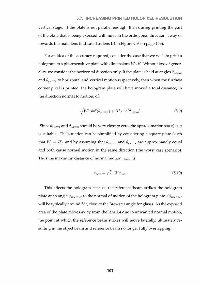
5.7. INCREASING PRINTED HOLOPIXEL RESOLUTION
vertical stage. If the plate is not parallel enough, then during printing the part
of the plate that is being exposed will move in the orthogonal direction, away or
towards the main lens (indicated as lens L4 in Figure C.6 on page 159).
For an idea of the accuracy required, consider the case that we wish to print a
hologram to a photosensitive plate with dimensionsW×H . Without loss of gener-
ality, we consider the horizontal direction only. If the plate is held at angles θx,error
and θy,error to horizontal and vertical motion respectively, then when the furthest
corner pixel is printed, the hologram plate will have moved a total distance, in
the direction normal to motion, of:
√W 2 sin2(θx,error) +H2 sin2(θy,error) (5.9)
Since θx,error and θy,error should be very close to zero, the approximation sin(x) ≈ x
is suitable. The situation can be simplified by considering a square plate (such
that W = H), and by assuming that θx,error and θy,error are approximately equal
and both cause normal motion in the same direction (the worst case scenario).
Thus the maximum distance of normal motion, zmax, is:
zmax =√
2 ·Wθerror (5.10)
This affects the hologram because the reference beam strikes the hologram
plate at an angle φreference to the normal of motion of the hologram plate. (φreference
will be typically around 56◦, close to the Brewster angle for glass). As the exposed
area of the plate moves away from the lens L4 due to unwanted normal motion,
the point at which the reference beam strikes will move laterally, ultimately re-
sulting in the object beam and reference beam no longer fully overlapping.
101
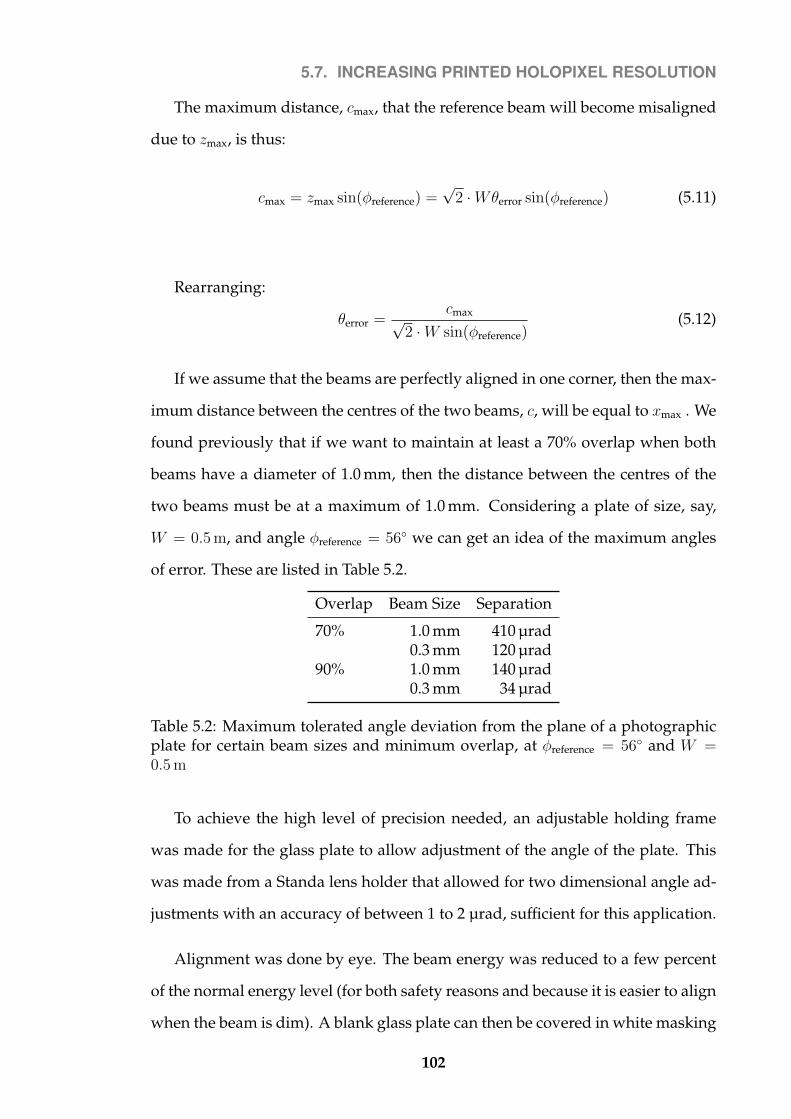
5.7. INCREASING PRINTED HOLOPIXEL RESOLUTION
The maximum distance, cmax, that the reference beam will become misaligned
due to zmax, is thus:
cmax = zmax sin(φreference) =√
2 ·Wθerror sin(φreference) (5.11)
Rearranging:
θerror =cmax√
2 ·W sin(φreference)(5.12)
If we assume that the beams are perfectly aligned in one corner, then the max-
imum distance between the centres of the two beams, c, will be equal to xmax . We
found previously that if we want to maintain at least a 70% overlap when both
beams have a diameter of 1.0 mm, then the distance between the centres of the
two beams must be at a maximum of 1.0 mm. Considering a plate of size, say,
W = 0.5 m, and angle φreference = 56◦ we can get an idea of the maximum angles
of error. These are listed in Table 5.2.
Overlap Beam Size Separation
70% 1.0 mm 410 µrad0.3 mm 120 µrad
90% 1.0 mm 140 µrad0.3 mm 34 µrad
Table 5.2: Maximum tolerated angle deviation from the plane of a photographicplate for certain beam sizes and minimum overlap, at φreference = 56◦ and W =0.5 m
To achieve the high level of precision needed, an adjustable holding frame
was made for the glass plate to allow adjustment of the angle of the plate. This
was made from a Standa lens holder that allowed for two dimensional angle ad-
justments with an accuracy of between 1 to 2 µrad, sufficient for this application.
Alignment was done by eye. The beam energy was reduced to a few percent
of the normal energy level (for both safety reasons and because it is easier to align
when the beam is dim). A blank glass plate can then be covered in white masking
102

5.8. 3D MODEL
tape, and placed in the holder, with the masking tape closest to the main lens
(where the emulsion would be located). It is best to use an actual hologram plate,
as it is important that the glass plate is of the same thickness as the hologram
plate that will be employed.
The plate was then moved (using computer control or otherwise) to one cor-
ner (meaning that the glass plate is moved so that the object and reference beams
are illuminating one of the corners of the plate). The reference beam mirror (la-
belled M2 in Figure 5.1 on page 92) can then be adjusted until the beams overlap,
judging this as best as possible by eye.
The glass plate is then moved (by computer control) so that the other corner is
exposed. If the beams no longer overlap completely, the angles are adjusted, and
the process repeated.
Although somewhat crude, this actually works fairly well in practice.
5.8 3D model
The produced holograms were based upon two different 3D models. The low
resolution holograms used a 3D model of the KDE mascot, Konqi. For the higher
resolution holograms, a greyscale, high contrast and high detail model was re-
quired. For this, the kind permission from Doug Ollivier was granted for the
non-commercial use of his model of a futuristic tank model.
The increase in holopixel resolution meant that higher resolution images of the
model are required. Additionally, the increase in pixels on the LCOS (1280×768
on the LCOS compared to 800×600 on the LCD) potentially means that more
rendered images can be used, to provide a greater depth of the field. The LCOS
is used in landscape orientation in the hologram printer, meaning that for single
parallax holograms, up to 1280 separate images are required, each rendered from
a slightly different angle. For full parallax, up to 1280×768 ≈ 1 million images
would be required.
103

5.8. 3D MODEL
To determine how to render the images from the 3D model for the horizontal
parallax case only, an intuitive approach can be taken. The scene needs to be
rendered from many different angles, producing an image for some discrete set
of angles. By moving the virtual camera along a virtual track, keeping the camera
pointed at the center of the scene, we can produce the required series of images.
However these images will need to be algorithmically distorted as each image is
taken at a different angle.
Instead, the camera was set to capture a view that was twice as wide as the
scene. The virtual camera was first calibrated such that its field of view was
equal to the field of view produced by the imaging lens system of the LCOS
onto the hologram plate. The camera was then placed at a distance such that
the scene took up exactly the whole of the right half of the view (see the scene
setup in Blender in Figure 5.4a on the next page). This established the start point
of the camera track (see the rendered image in Figure 5.4b). The camera was then
moved parallel to the scene into a position such that the scene took up exactly
the whole of the left half of the view. This established the last point of the camera
track (see Figure 5.4c).
A linear track was then made between these two points, discretized such that
Nimages number of images was produced. These images are then cropped with a
sliding window such that the new image has the same height, but half the width,
resulting in a series of Nimages images, all with the scene centered in each image
(see Figure 5.4d and Figure 5.4e). Since these images need to be cropped, it is
advantageous to be able to crop by an integer number of pixels to avoid the need
for interpolation. This means that the sliding cropping window must move by an
integer number, k, of pixels each time. Writing the cropped image width asWimage
pixels, the uncropped image width is thus 2Wimage. This gives us the restriction
that 2Wimage/k ∈ N∗ and that it is equal to the number of images, Nimages.
So the width of the uncropped images, 2Wimage, must be some integer multi-
ple of number of images rendered. The width of a rendered and cropped image,
104

5.8. 3D MODEL
(a) Setting up the scene in Blender
(b) Rendered left-hand side (c) Rendered right-hand side
(d) Cropped left (e) Cropped right
Figure 5.4: Rendered model images
105
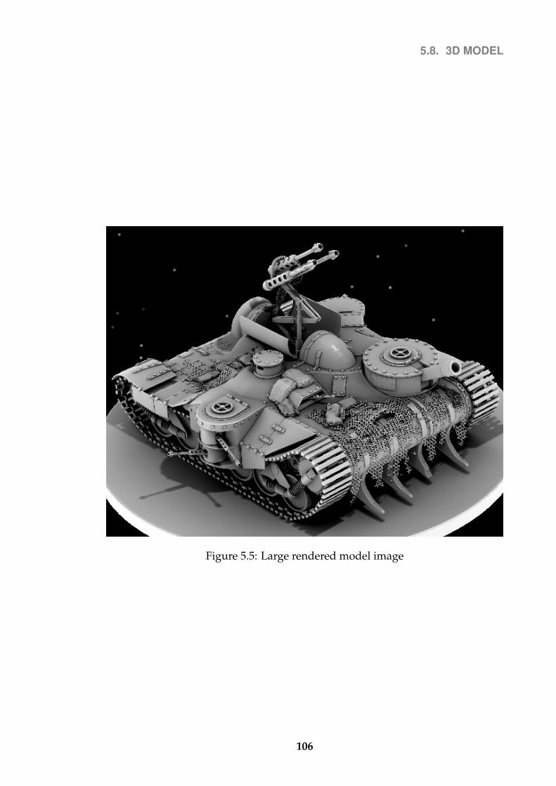
5.8. 3D MODEL
Figure 5.5: Large rendered model image
106

5.8. 3D MODEL
in pixels, also corresponds to the width, in holopixels, of the final printed holo-
gram. Likewise, the height of the rendered image corresponds to the height, in
holopixels, of the final printed hologram.
A further restriction can be made from the LCOS resolution. Consider the
holopixel at coordinate (x, y) being printed, with x and y in units of pixels. The
LCOS must display an image such that the same (x, y) coordinate pixel from each
image is mapped to a pixel on the LCOS. The solution can be simplified by
imposing the restriction that the effective5 horizontal resolution of the LCOS is
Wlcos = mNimages where m ∈ N∗.
To summarize, the following restrictions were imposed in order to optimize
the code:
Nimages =2Wimage
k(5.13)
Nimages =Wlcos
m(5.14)
Himage = Hhologram (5.15)
Wimage = Whologram (5.16)
WhereNimages is the number of rendered images,Wimage andHimage are the width
and height respectively of the cropped image, Wlcos is the effective width of the
LCOS, Whologram and Hhologram are the effective width and height in pixels respec-
tively of the hologram, and m and k are arbitrary non-zero natural numbers.
To print the test model for the purpose of evaluating the printer, a holopixel
size of approximately 0.3 mm was used. A resolution of 0.3 mm between pixel
centers is approximately 85 Dots Per Inch (DPI), similar to that of the resolution
of a computer screen. To aid in the visual evaluation of the completed hologram,
however, the distance between the pixels was increased to 0.5 mm, leaving a gap
between each pixel (See Figure 5.7 on page 111).
5Sometimes it is advantageous to only use a portion of the LCOS screen, hence the prependedqualifier ’effective’.
107

5.8. 3D MODEL
The hologram was printed on a large Slavich VRP-M glass plate of dimen-
sions 60 cm×40 cm in landscape. With a 0.5 mm inter-pixel spacing, the maxi-
mum width and height of the hologram in pixels is thus:
Whologram ≤ 60 cm÷ 0.5 mm/pixel = 1200 pixels (5.17)
Hhologram ≤ 40 cm÷ 0.5 mm/pixel ≈ 800 pixels (5.18)
For the Brillian LCOS BR1080HC display system with a resolution of 1280×768
used in landscape format, Wlcos = 1280. To produce a slightly brighter holo-
gram, the hologram replay viewing window was reduced by reducing the effec-
tive width of the LCOS to 984 pixels. This particular size was chosen to allow the
image size to be nice resolution.
Rearranging Equation (5.13) and Equation (5.14) on the previous page:
Wimage =k
2mWlcos (5.19)
Setting m = 2 & k = 5:
1230 =5
4× 984 (5.20)
Nimages =2× 1230
5= 492 (5.21)
An image height of 960 was chosen. 492 images were thus rendered at 2460×960
and cropped to 1230×960 using the program listed in Appendix A.
A single rendering of the test model at this resolution took approximately five
hours to do on a single CPU PC. Extrapolating, this would take a total rendering
time of 1280×5 hours = 1 month. To reduce this time, the rendering farm com-
pany ResPower was used, completing the render in just under 24 hours. If max-
imum resolution and maximum depth was used instead, the rendering would
have taken an estimated 1.5 years of rendering time - around a week on the Re-
sPower rendering farm.
108

5.9. ANALYSIS
5.9 Analysis
After several attempts, a successful bright hologram was produced. With just
over a million pixels, the hologram took around 11 hours to print at rate of 30
pixels per second. This speed was experimentally pushed up to 42 pixels per
second for smaller holograms without noticeable problems.
To protect and display the hologram, the hologram was printed back to front
and then the emulsion side spray-painted black. A few different brands of spray
paint were tested to find one that not harm the emulsion. The best performing
paint was a cheap quick-dry car matt-black spray-paint. This caused the holo-
gram to color shift slightly, but had no noticeable adverse affect on the brightness.
Figure 5.6 on the following page shows a photograph of the final hologram.
This was taken with a 0.625 second exposure and a f/4.2 aperture. The ghost-like
artifacts are due to reflections from the glass, and are not prominent when viewed
by eye.
A single attempt was made to try to print with an inter-pixel size of 0.28 mm.
This produced a dim hologram that is visible to the eye but too dim to photo-
graph with a standard digital camera. This failure was most likely due to a bad
alignment of the object and reference beams on the holographic emulsion, and
further experimentation is required.
Figure 5.7 on page 111 shows an enlarged portion of the hologram. Notice that
the pixels are perfectly aligned in both axes (The tilt of the y-axis is just due to the
angle of the hologram when the photograph was taken. The axes are orthogonal.)
The spacing between the pixels has been left slightly larger than the actual pixel
size (Approximately 0.5 mm spacing) to make such analysis of the final hologram
easier.
109

5.9. ANALYSIS
Figure 5.6: High resolution (0.3 mm in diameter pixels) hologram of futuristictank. Some of the low contrast and low detail are due to the difficulty in capturingthe image with the camera.
110

5.9. ANALYSIS
Figure 5.7: Zoomed in on a small section of the high resolution hologram. Blurri-ness and artifacts are due to the difficulty in capturing the image with the camera.
111

5.10. SUMMARY
5.10 Summary
Various printing speed and resolution improvements to the digital direct-write
monochromatic hologram printer described in Chapter 3 were investigated and
implemented. The printing speed was successfully increased from 4 holopixels
per second to 40 holopixels per second through a variety of software and me-
chanical improvements along with a newer design of a laser power supply. The
printing resolution of holopixels was increased, with the holopixel diameter re-
duced from 1.0 mm to 0.3 mm - a factor of ten increase in resolution. The render-
ing of the input images was also discussed along with the restrictions required
for optimal holograms.
It was found that achieving the required high precision timing on a normal PC
for printing at 40 holopixels per second is possible but that further improvement
to printing speed would require a realtime operating system with high perfor-
mance hardware timers.
A demonstration of the final results is given in Figure 5.4a on page 105.
112

6Temperature-energy feedback
This chapter details the custom energy meter and heating system that was built to
improve the pulse to pulse laser energy stability by reducing laser mode beating.
A computer controlled heating system was created for adjusting the position of
the laser cavity rear mirror and was driven by a temperature-energy feedback
algorithm. The heating system was additionally used for maintaining a constant
temperature within the laser, to further help with stability. The effectiveness of
these improvements is determined.
6.1 Problems with laser instability
The particular laser investigated for use in the hologram printer is an infrared
1064 nm passively Q-switched long-cavity pulsed laser. The fundamental beam
has a frequency of 1064 nm beam which is frequency doubled to 532 nm (visible
green). The laser produces up to 50 pulses a second, each with 50 ns pulse width,
113

6.1. PROBLEMS WITH LASER INSTABILITY
and has a single TEM00 beam mode. The full technical specifications are given in
Appendix H.
The pulse energy was found to be unstable with between a 10% to 30% pulse-
to-pulse standard deviation in energy. This produces noticeable defects in the
replay of the printed hologram (as seen in Figure 3.19 on page 68), as the pix-
els are printed with different energy densities. This in turn affects the hologram
because the maximum diffraction efficiency of the final developed hologram is
a function of the incident energy density [78]. The exact nature of this function
varies between emulsions, but typically has a peak diffraction efficiency at some
particular energy density with a gradual decrease in diffraction efficiency with
increasing energy density, as shown in Figure 6.1 on the following page. The
energy stability required from the hologram printer laser is thus dependant on
the slope of this curve. By inspection of the relationship between energy density
and diffraction efficiency, and from experience of printing holograms, we found
that for the Slavich monochromatic emulsion Slavich VRP-M and the panchro-
matic Slavich PFG-03C, a pulse-to-pulse standard deviation of less than 10% is
not noticeable under normal viewing conditions.
It is worth mentioning that the contrast of the image is related to the inter-
ference term which relies on the relative intensities of the reference and object
beams. Since the two beams originate from the same laser source, the relative
intensities remain unaffected by laser instability.
The pulse-to-pulse standard deviation changes due to uncontrolled changes
to optical length of the laser resonance cavity due to temperature fluctuations,
changes in moisture, etc[79]. The laser is designed to be locked to a certain mode
by the combination use of a thin and thick etalon. However if the cavity optical
length changes sufficiently, a second mode frequency can be selected. If multiple
mode frequencies can coexist in the resonance cavity, they compete, producing
mode beating which causes a drop in the beam intensity. It is this drop in the
beam intensity that can cause some pixels on the final hologram image to appear
114

6.1. PROBLEMS WITH LASER INSTABILITY
50 75 100 12530.0%
35.0%
40.0%
45.0%
50.0%
Exposure (microJoules/cm2)
Diff
ract
ion
effic
ienc
y
Figure 6.1: Diffraction efficiency curve for Slavich VRP-M monochromatic emul-sion suitable for holography at 532 nm (Data source: [64]). Diffraction efficiencycurves for other emulsions are similar[64, 78].
much dimmer than others in replay. Severe mode beating can often be observed
to the naked eye as an occasional flickering of the beam.
We have argued for the need for improved energy stability in order to produce
high quality holograms, and that the reason that the laser is unstable is because
it uses a long resonance cavity that can change its effective optical size due to
temperature, moisture, etc. fluctuations.
This was approached on two fronts. The first was to try to limit the temper-
ature fluctuations. The laser was enclosed in a case with a heated breadboard.
The breadboard was heated with a temperature feedback system that continually
measures and heats the breadboard to maintain a stable temperature.
The second step is to have an active way to adjust the cavity length size. By im-
plementing a system that can change the physical cavity length, we can counter
changing air densities, and other changes, in an attempt to keep the optical cavity
length constant.
To achieve this, the rear mirror of the cavity was mounted onto one end of a
metal block. The other end was mounted in a holder for mounting in the laser.
Two resistors were affixed to the metal block to provide the ability to heat the
block, along with a thermiresistor to measure the temperature of the block. When
115

6.2. CUSTOM ENERGY METER
the metal block is heated the block expands, adjusting the position of the rear mir-
ror. In this way the position of the rear mirror can be adjusted to high precision
(see Equation (6.2)) to compensate for uncontrolled resonance length variations.
Aluminum was chosen for the material of the metal block. Aluminum has a
coefficient of linear thermal expansion of 23× 10−6 K−1. As we will see, the tem-
perature of the block can be controlled to within an accuracy of 0.01 ◦C. For an
aluminum block of length 1.5 cm, the thermal expansion for a change in temper-
ature of 0.01 ◦C is:
∆L = 1.5× 10−3 m× 23× 10−6 K−1 × 0.01 K (6.1)
≈ 0.35 nm (6.2)
This is of sufficient accuracy for a fundamental mode of 1064 nm.
Rather than attempting to determine the optical cavity length at any given
time, in order to compensate for its changes, the energy can measured instead
and used as the basis for adjusting the position of the rear mirror. A feedback sys-
tem was implemented to monitor the beam energy. If temperature/moisture/etc
fluctuations cause the optical cavity length to change, the beam energy changes,
and the feedback system can adjust the position of the rear block to compensate.
Both the energy-feedback system and the breadboard heating system require
a heating and monitoring component, with its own feedback system, to heat to a
given temperature. The same system was used for both of these needs, and will
be hereby referred to as the Digital Temperature Controller (DTC).
6.2 Custom energy meter
To control the energy stability, a computerized system is required to measure
the energy in each beam pulse. For this task, a custom energy meter was built.
Although off-the-shelf energy meters exist, a simple and cost effective device was
116

6.2. CUSTOM ENERGY METER
required that worked at low energies (of the order of micro Joules). Since it was
to be fixed in place and communicate only to a computer, a display etc was not
required. Since the energy stability is the key piece of information that is required,
overly accurate calibration and preciseness was also not required.
A general overview of the custom energy meter is discussed below, followed
by a discussion of methods for diverting the energy beam into the custom energy
meter. Next the calibration of energy meter is explained, concluding with a com-
parison of energy readings with an off-the-shelf energy meter from the company
Ophir.
6.2.1 Overview of custom energy meter
A small portion of the beam to be measured is diverted onto the surface of an
awaiting photodiode. The 50 ns laser pulse used is too short to measure directly,
so current from the photodiode is collected onto the plates of a capacitor. The
capacitor is then allowed to leak to ground through a resistor. The capacitor leaks
in a consistent way, with the voltage across it following a very specific profile
which is determined by the initial charge collected. By using an Analogue-Digital
(A-D) converter to measure the voltage across the capacitor with time and timing
how long it takes for the capacitor to discharge, the initial collected energy can be
deduced. From that, with calibration, we can deduce the energy that was in the
incident laser pulse.
6.2.2 Methods for diverting beam
Since the feedback system needs to be working continually, a real-time monitor-
ing system needs to be put in place; blocking the beam in order to measure its
energy is clearly not desirable. As stated before, the laser has a fundamental fre-
quency of 1064 nm which is frequency doubled to 532 nm. Either of these are
suitable for monitoring the energy, but the visible second-harmonic (532 nm) is
117

6.2. CUSTOM ENERGY METER
the more obvious candidate. There are various methods for diverting a small
amount of the beam in order to measure the energy. Two different approaches
were evaluated. The first approach tried was to measure the back leakage from
one of the various 90◦ reflective mirrors used (Figure 6.2a).
D
(a) Measuring the leakage from acoated mirror
D
(b) Using a coated wedge to’steal’ a portion of the beam
Figure 6.2: Two possible layouts to deflect energy to the detector, D.
The mirrors, although coated, are not 100% perfect – a small amount of the
beam energy transmits (‘leaks’) through the mirror and would be normally dis-
carded.
The second approach tried used a thin glass wedge coated on one side, placed
in the beam. The wedge reflects around 3% of the beam energy to the waiting
photo-diode (Figure 6.2b) 1.
The second approach used a thin glass wedge two glass right-angled coated
wedges, placed next to each other in the beam. The wedge reflects around 3% of
the beam energy to the waiting photo-diode (Figure 6.2b).
The calibration of the energy meter is discussed later, but the results regarding
the method for deflection are mentioned here, for the sake of continuity.
The first method was found to give unreliable results. The percentage of leak-
age through the mirror was not predictable with time. This can be demonstrated
by a plot of the energy readings taken from the off-the-shelf pre-calibrated Ophir
meter and comparing them against the readings from the custom energy detec-
1In practice, two right-angled coated wedges were used, with one rotated by 180◦, to act as asingle wedge.
118

6.2. CUSTOM ENERGY METER
tor. There should be a one-to-one mapping between the two sets of readings with
some small margin of error. Instead there appears to be two distinct clusters, as
can be see in Figure 6.32.
Comparison of energy readings, using mirror leakage
1.85
1.87
1.89
1.91
1.93
1.95
1.97
1.99
1.5 1.55 1.6 1.65 1.7 1.75 1.8 1.85 1.9 1.95 2
Custom meter (mJ)
Oph
ir m
eter
(m
J)
Figure 6.3: Comparison of energy readings from the Ophir energy meter and thecustom energy meter, obtained for mirror-leakage.
The second method, to use a thin coated wedge, was found to give more reli-
able results. Testing shows a strong, and time-constant, correlation between the
energy reading given by the custom energy meter and the energy reading given
by the Ophir energy meter. All future graphs and values are given for this second
method, unless otherwise noted.
6.2.3 Calibrating custom energy meter
The 50 ns laser pulse used is too short to measure directly, so current from the
photodiode is collected onto the plates of a capacitor. The capacitor is then al-
lowed to leak to ground through a resistor. The capacitor leaks in a consistent
way, following a very specific profile which is determined by the initial charge
2Note that the scale for the readings from the custom energy meter are somewhat arbitrary,given that no sensible calibration can be obtained
119

6.2. CUSTOM ENERGY METER
collected. By using an A-D converter to measure the voltage across the capacitor
with time and timing how long it takes for the capacitor to discharge, the initial
collected energy can be deduced. From that, with calibration, we can deduce the
energy that was in the incident laser pulse.
To calibrate the photo-detector, an off-the-shelf calibrated energy meter was
placed in the optical path of the 532 nm beam and the beam energy adjusted to
calibrate and check the photo-detector software. The energy meter triggers send-
ing the voltage reading data to the PC when the voltage suddenly spikes – i.e. at
the start of a pulse. The first few readings saturate the A-D converter and just re-
turn the maximum value – 4096. Then as the voltage drops we measure the decay
curve. Two example pulses with different energies are shown in Figure 6.4.
Measured voltage across capacitor against time
0
512
1024
1536
2048
2560
3072
3584
4096
1 3 5 7 9 11 13 15 17 19 21 23 25 27 29 31 33 35 37 39 41 43 45 47
Reading number (proportional to time)
Pot
entia
l diff
eren
ce a
cros
s ca
paci
tor
Measured: Pulse 1 Measured: Pulse 2
Figure 6.4: Measured voltage across the energy meter’s capacitor against time,after a pulse (Arbitrary units)
To determine the energy from this curve, the values between 2400 and 1000
were considered only.
The potential difference across the capacitor curve follows a characteristic ca-
120

6.2. CUSTOM ENERGY METER
pacitor decay curve of:
Vt = V0e−t/RC (6.3)
The energy in capacitor is related to the potential difference across the capaci-
tor by the equation:
E =1
2CV 2 (6.4)
So indicating initial energy as E0 we obtain:
Vt =
√2E0
Ce−t/RC (6.5)
Using variable substitution of A = 2C
and k = 2RC
:
Vt =√AE0e
−kt/2 (6.6)
By using the data measured for the voltage across the capacitor after a single
pulse and setting E0 to one we can use the least squares algorithm to determine
the best fitting A and k constants. Repeating this process for many pulses, differ-
ent values A will be obtained, but the k values will be very similar. The average
value of k thus determines the calibration k constant. An arbitrary value forA can
be chosen as A simply sets the calibration scale of the energy. After calibration,
we obtain a fit as shown in Figure 6.5 on the next page.
With the now determined values of A and k in hand, it is useful to rearrange
the Equation (6.6) to obtain the energy in the pulse in terms of the measured
potential differences, as so:
E0 = V 2t · A−1ekt (6.7)
So using the measured values for the voltage across the capacitor, Vt, and our
determined values for k and A, the initial energy (measured on some arbitrary
scale) of the pulse, E0, can be found.
An estimate for the energy for any pulse can now be determined. Using an
121

6.2. CUSTOM ENERGY METER
Measured and theoretical voltage across capacitor
0
512
1024
1536
2048
2560
3072
3584
4096
4608
5120
5632
6144
1 3 5 7 9 11 13 15 17 19 21 23 25 27 29 31 33 35 37 39 41 43 45 47
Reading number (proportional to time)
Pot
entia
l diff
eren
ce a
cros
s ca
paci
tor
Measured: Pulse 1 Measured: Pulse 2 Theoritical: Pulse 1 Theoritical: Pulse 2
Figure 6.5: Measured and theoretical voltage curve of capacitor for energy meter
energy meter that has already been calibrated, the value of A can be determined
such that our energy is measured in Joules.
A comparison of the energy measured by this device against the energy mea-
sured by an off-the-shelf energy meter by the company Ophir is given in Fig-
ure 6.6 on the next page. For this graph the photodiode was using the energy
leakage from a mirror. The two graphs do not fit perfectly, although it is ade-
quate for the energy-temperature feedback system.
122
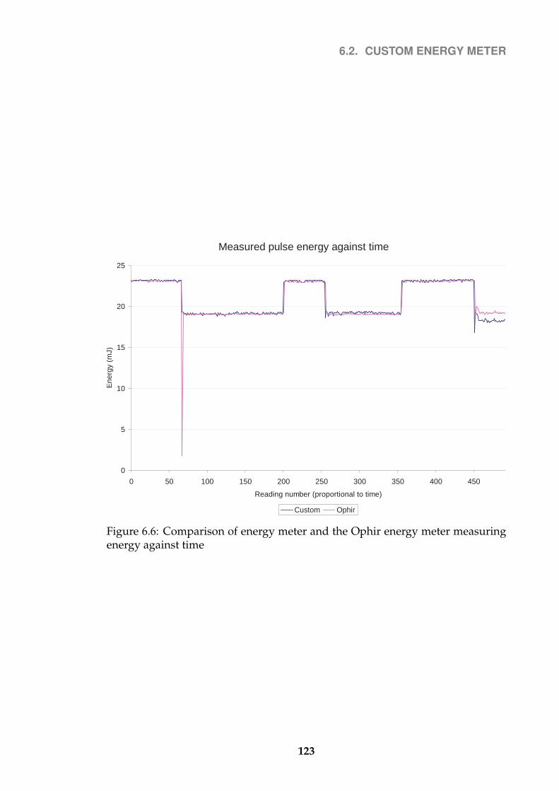
6.2. CUSTOM ENERGY METER
Measured pulse energy against time
0
5
10
15
20
25
0 50 100 150 200 250 300 350 400 450
Reading number (proportional to time)
Ene
rgy
(mJ)
Custom Ophir
Figure 6.6: Comparison of energy meter and the Ophir energy meter measuringenergy against time
123
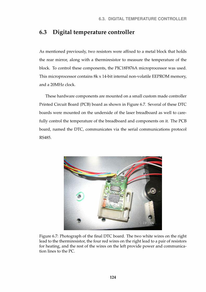
6.3. DIGITAL TEMPERATURE CONTROLLER
6.3 Digital temperature controller
As mentioned previously, two resistors were affixed to a metal block that holds
the rear mirror, along with a thermiresistor to measure the temperature of the
block. To control these components, the PIC18F876A microprocessor was used.
This microprocessor contains 8k x 14-bit internal non-volatile EEPROM memory,
and a 20MHz clock.
These hardware components are mounted on a small custom made controller
Printed Circuit Board (PCB) board as shown in Figure 6.7. Several of these DTC
boards were mounted on the underside of the laser breadboard as well to care-
fully control the temperature of the breadboard and components on it. The PCB
board, named the DTC, communicates via the serial communications protocol
RS485.
Figure 6.7: Photograph of the final DTC board. The two white wires on the rightlead to the thermiresistor, the four red wires on the right lead to a pair of resistorsfor heating, and the rest of the wires on the left provide power and communica-tion lines to the PC.
124

6.4. TEMPERATURE FEEDBACK ALGORITHM
6.4 Temperature feedback algorithm
The Digital Temperature Controller has one input (the current measured temper-
ature) and one output (whether to heat or not). There is a time delay between
switching on the heating and the new temperature registering on the thermome-
ters. This is because it takes time for the resistors to heat up and time for the heat
to conducted through the material. This means that if we simply heat until we
measure the required temperature and then switch of the heating, we will find
that the measured temperature continues to climb, overshooting the target tem-
perature. If we are too cautious in heating then we risk taking a much longer time
to heat than necessary.
This can be solved by using a Proportional Integral Derivative (PID) controller
algorithm [80]. This is a general purpose control-loop fedback algorithm that is
widely used in industrial control systems.
The PID controller attempts to correct the error between a measured input
variable (the temperature) and a desired target (the temperature we want to heat
to) by calculating and then outputting a corrective action that can adjust the pro-
cess accordingly (by heating).
There are 3 steps to this algorithm.
The first step is a Proportional response that changes the output proportion-
ally to the current temperature error. The constant of proportionality is labelled
Kp.
The second step is an Integral response that changes the output based on the
accumulated instantaneous temperature readings over time. The integral gain
constant is labelled Ki.
The final step is a Differential response that changes the output proportionally
to the rate of change of the temperature error. The differential gain constant is
labelled Kd.
125

6.4. TEMPERATURE FEEDBACK ALGORITHM
Using a fairly standard adaptation, the integral response was changed to limit
the time period over which the integral is done. This is omitted from the pseudo
code for sake of clarity.
This algorithm was implemented in the computer language C and run on
the Digital Temperature Controller boards. The pseudo code is shown in Algo-
rithm 2.
∆T0 = 0;1
t = 1;2
repeat3
∆Tt = T Target − Tt;4
Pt = Kp ·∆Tt;5
It = It − 1 +Ki ·∆Tt ·∆t;6
Dt = Kd ·∆Tt −∆Tt−1/∆t;7
output = Pt + It +Dt;8
heat output;9
wait for time ∆t;10
t = t+ 1;11
until finished ;12
Algorithm 2: Digital Temperature Controller feedback using PID algorithm
Calibration of the parameters Kp, Ki and Kd was done manually. They are
dependant upon many factors – mechanical setup, size of the mechanical blocks,
thermal insulation, heating resistor used, etc. The resistors were tested against
various target temperature functions and the optimal set of parameters chosen.
The time period across which to integrate was limited to the previous 32 seconds.
The final values decided on were:
Kp = 0.7
Ki = 0.02
Kd = 0.7
(6.8)
This results in the fit shown in Figure 6.6 on page 123.
126

6.5. TEMPERATURE FEEDBACK SYSTEM ON REAR MIRROR
6.5 Temperature feedback system on rear mirror
As mentioned before, the rear mirror in the laser cavity was mounted on one
end of a metal block whose other end is mounted in a holder. One of these DTC
boards was used to control the temperature of this rear mirror metal block.
This gives a response such as that shown in Figure 6.8 on the following page.
The light gray line indicates the target temperature, T Target, as a function of time.
The black line shows the measured temperature Tt as a function of time. To in-
crease the temperature, the system responds rapidly. It takes approximately 20
seconds to increase the temperature by 4 °C. Cooling down requires simply wait-
ing for the excess heat to be carried away, requiring about one and a half minutes
to decrease the temperature by 4 °C.
Such large temperature changes are not, however, useful to us for any normal
operation. It is shown simply to check the behavior of the system.
We can use the same temperature system to control the temperature of the
bread board.
Figure 6.9 on the next page shows the same system working for heating the
breadboard. The target temperature is set here at 33 °C, and kept constant. This
shows that there was a large source of noise arising from somewhere, but despite
the noise the feedback system still managed to cope exceptionally well. After
fixing the various noise problems, the temperature looks like that shown in Fig-
ure 6.10 on page 129. The standard deviation of the temperature is a lot better
than it might appear from the graph – around 0.02%. For the holographic printer,
the temperature of the breadboard is kept at 37.50±0.02 °C.
127

6.5. TEMPERATURE FEEDBACK SYSTEM ON REAR MIRROR
Feedback reaction to extreme temperature changes
33.5
34
34.5
35
35.5
36
36.5
37
37.5
38
38.5
00:00 03:30 07:00 10:30
Time (Minutes:Seconds)
Tem
pera
ture
(°C
)
Rear Mirror Temperature Rear Mirror Target Temperature
Figure 6.8: Digital Temperature Controller PID response to target temperaturechanges
Feedback reaction to noise in temperature readings
32
32.5
33
33.5
34
34.5
00:00 03:30 07:00 10:30
Time (Minutes:Seconds)
Tem
pera
ture
(°C
)
Breadboard Temperature Breadboard Target Temperature
Figure 6.9: Digital Temperature Controller PID response to noise in temperaturereadings
128

6.6. DTC-PC COMMUNICATION
Breadboard temperature against time
37
37.1
37.2
37.3
37.4
37.5
37.6
37.7
37.8
37.9
38
18:43 19:55 21:07 22:19 23:31 00:43
Time (Hours:Minutes)
Tem
pera
ture
(°C
)
Figure 6.10: Breadboard temperature against time
6.6 DTC-PC communication
So now we have a way of maintaining a given temperature. The Digital Tem-
perature Controller (DTC) board works independently to maintain the set target
temperature. To set the target temperature, the DTC board talks to the computer
via a serial communication protocol. The DTC boards use the RS485 serial proto-
col, produced by Electronics Industry Alliance (EIA). This protocol uses a voltage
differential signal increasing its immunity against signal noise and suitable for a
multi-point communications network. It also offers protection against data col-
lision (multiple nodes accidentally talking simultaneously) and bus fault prob-
lems. The protection against signal noise is particularly important for the appli-
cation of a DTC in a hologram printer because of the high voltage power supplies,
flash lamps and other high voltage equipment that is present in the environment
around the DTC communication wires.
RS485 also allows for multiple systems on a single wire. This allowed us to
129

6.6. DTC-PC COMMUNICATION
have multiple DTCs as well as other subsystems all connected via the same wires.
For our purposes it was convenient to have all the data wires join together and
feed into a USB-to-serial converter, and then plug the Universal Serial Bus (USB)
converter into a PC.
For the higher level communication protocol, a custom protocol was devel-
oped. Each DTC, as well as other subsystems, were considered as separate nodes.
Each node was given a unique number from 0 to 254. The node number 255 was
reserved to indicate all nodes. Each node thus responded only to commands ad-
dressed to their own node number, or to the node number 255.
RS485 is half duplex and only allows one device to be talking at a time – to
prevent cross talk. The protocol is robust enough to recover from accidentally
cross talk.
To make the protocol simple, the PC acted as a master, and the nodes act as
slaves – only communicating in reply to a message. At start up, the PC can send a
‘ping’ message to each node identification number (ID) number in turn. If a node
sees a ping message with its ID on it, it replies. If there is no reply within some
timeout period then the PC knows that there is no node connected with that ID.
In this way the PC can ‘scan’ the bus looking for devices.
Every second, or so, the PC sends a message to the first device that it knows is
connected asking for the current temperature. It then waits for a reply (or a time-
out in case of an error) before asking the next device for its current temperature.
In this fashion the PC can be kept updated about the current temperatures
of all the parts of the laser. At any time the PC can send a message to set the
temperature.
To set a node ID on a DTC or to reprogram a node, a single node must be
connected to the computer by itself. Then the node ID 255 can be used to com-
municate to it and to reprogram it.
130

6.7. TEMPERATURE-ENERGY FEEDBACK
6.7 Temperature-energy feedback
We now have the components required to measure the current beam energy and
to adjust the cavity length by heating and thus expanding a small block that the
rear mirror is attached to.
The aim now is to adjust the rear mirror as needed in order to try to maximise
the beam energy and minimize the point-to-point standard deviation of the beam
energy.
To first get a qualitative feel for how the energy depends on the cavity length,
a temperature scan was performed. This changes the temperature of the metal
that the rear mirror is mounted on, and hence changes the cavity size. The first
attempt of an energy scan was run for just over twenty hours, with the results
shown in Figure 6.11.
Energy against time during temperature scan
1.6
1.61
1.62
1.63
1.64
1.65
1.66
1.67
1.68
1.69
0 2 4 6 8 10 12 14 16 18 20
Time (Hours)
Ene
rgy
(mJ)
0
5
10
15
20
25
30
35
40
45
Tem
pera
ture
(°C
)
Energy (mJ) Temperature (°C)
Figure 6.11: Energy against time in rear mirror position scan over 20 hours
This shows that something has gone wrong. The energy increases with the
temperature (and hence shortening of the cavity) to within the limits of the heat-
131

6.7. TEMPERATURE-ENERGY FEEDBACK
ing system. This means that the cavity is misaligned, and the rear mirror is far
away from the optimal position.
To fix, the rear mirror temperature is set to a middle-of-the-range temperature.
The laser was opened up and the rear mirror’s position mechanically adjusted,
using an energy meter to recalibrate it.
Despite this being a laser alignment mistake, we mention it here because this
is a useful way to tell if the laser is correctly aligned.
To control the energy, we must control the rear mirror position, and thus the
temperature of the block it is mounted on. However how can we know whether
to heat or cool the block in order to increase the energy?
Initially a simple discrete algorithm was used to decide whether to heat or
cool. It was heated initially, say, until the energy decreased. It then cooled (i.e.
not heated), expecting that the energy would thus increase again. It continued to
cool until the energy decreased again.
This was found to be too sensitive to point-to-point variations in the energy,
even if some average was taken. It would oscillate between heating and cooling,
getting stuck in local minima and responding to insignificant noise.
Instead, a more robust, but still discrete, algorithm based on that indicated in
Figure 6.12 on the following page was used. This algorithm requires the energy
to drop twice in succession in order to cause the temperature to change.
To improve the algorithm, the energy standard deviation was also looked at.
As the standard deviation increases, so does the amount that the temperature is
increased or decreased by. This increases its ability to get out of local minima.
When the energy has dropped a lot and cavity is mode beating, the energy can
become highly unstable, meaning that algorithm in Figure 6.12 on the next page
can no longer work. By having a high standard deviation causing a large change
in temperature, it allows us to ‘jump out’ of the bad mode beating region.
132

6.7. TEMPERATURE-ENERGY FEEDBACK
Heat Cool
Heat Cool
∆E < −τ
∆E > τ
∆E < −τ
∆E > τ
∆E < −τ ∆E > τ ∆E < −τ∆E > τ
|∆E| < τ|∆E| < τ
|∆E| < τ|∆E| < τ
Figure 6.12: Energy temperature feedback algorithm for change of energy ∆Eand threshold τ .
This algorithm was found to perform very well, as shown by Figure 6.13
on the following page. The point-to-point standard deviation remains less than
0.3 mJ (approx 3% of the beam energy) for the vast majority of the time, well
within acceptable limits for hologram printing, as Figure 6.14 on the next page
shows. The figure shows peaks of high standard deviation, but these were all
below 10% standard deviation, producing no noticeable effects to the naked eye
on the final hologram. Note that the square wave appearance of the beam energy
is just due to a Neutral Density Filter being placed in the beam at arbitrary times,
just to check that the beam energy is monitored over a range of energies and that
no hysteresis effects are present. Also note that the graph indicates that Ophir
meter has a glitch at around reading number 60 that was not picked up on the
custom energy meter. The reason for this was not determined.
133

6.7. TEMPERATURE-ENERGY FEEDBACK
Measured pulse energy against time
15
16
17
18
19
20
21
22
23
24
0 1 2 3 4 5 6 7 8 9 10 11 12 13 14 15 16
Time elapsed (seconds)
Ene
rgy
(mJ)
Custom Ophir
Figure 6.13: Second harmonic (532 nm) pulse energy with active feedback
Pulse energy and standard deviation against time, with temperature feedback
0
2
4
6
8
10
12
14
18:43 19:55 21:07 22:19 23:31 00:43
Time (Hours:Minutes)
Ene
rgy
(mJ)
0
0.1
0.2
0.3
0.4
0.5
0.6
0.7
0.8
0.9
1
Poi
nt-t
o-po
int s
tand
ard
devi
atio
n (m
J)
Energy (mJ) Std. Dev of Energy
Figure 6.14: Second harmonic (532 nm) pulse energy with active feedback show-ing standard deviation
134

6.8. SUMMARY
6.8 Summary
Instability in the laser energy output resulted in printed holograms having dim
or missing pixels upon replay. A temperature control system was developed, and
used to control the laser breadboard temperature. In addition, the temperature
control system was used to adjust the position of the laser resonance cavity’s
rear mirror. This was coupled with an energy monitoring system and a PC to
provide an active feedback system to stabilize the energy. Two different methods
were investigated for diverting the beam energy into energy monitoring system,
with the glass beam wedge being the resulting preferred method. The energy
monitoring system was designed with the goal of being unobtrusive, cheap, and
accurate enough for use in the feedback system. It succeeded at achieving all of
these aims.
Using the active feedback for adjusting the position of the rear mirror based
on the energy gave us a much more stable beam. The pulse-to-pulse standard
deviation was reduced from over 10% to less than 3%, removing visual artifacts
from the printed holograms. The Digital Temperature Controller was found to re-
act fast enough for the requirements of a digital hologram printer, and performed
satisfactory.
135

7Conclusion and future work
7.1 Conclusion
This thesis researched and developed a direct-write pulse-laser hologram printer
design suitable for recording white-light viewable reflection holograms in an off-
axis geometry.
Chapter 3 examined the design of a one-step monochromatic hologram printer
capable of producing white-light viewable transmission holograms created with
the aid of an LCOS display system and printed in a dot-matrix sequence. The
lens system was analyzed and documented in detail, with a particular focus on
the microlens array system. The magnification of the object beam aperture due to
the afocal telescopic reversing lens system, combined with an upstream microlens
array system, was determined based upon a matrix method of lens analysis.
An optimal range of positions was analytically determined for each of the
three rectangularly-packed microlens array of differing lenslet size and lenslet
136

7.1. CONCLUSION
curvature. While the overall fidelity of the hologram was demonstrated to be sen-
sitive to the microlens array position, in their respective optimal positions there
was no significant difference between the three different microlens arrays tested
in terms of image fidelity, contrast and speckle. This implies that the contrast,
diffraction efficiency and depth of view of the hologram’s replay image will not
be significantly affected by the choice in the microlens array employed, to within
the range tested.
Chapter 4 analyzed the unwanted side effects of the angular intensity distri-
bution of a hologram pixel, using a ’White Logo’ hologram for case study. A
visible ’ghosting’ effect was demonstrated to be significantly reduced by apply-
ing a linear formula whose parameters were determined from either a grayscale
image of the hologram or by considering each color channel (in RGB color space)
separately. This correction can be applied as a pre-processing operation before
printing holograms in order to reduce ghosting in the final image. Additionally,
the artists can be warned when such effects may occur.
Chapter 5 examined methods for increasing both the printing speed and res-
olution of the hologram printer based upon increasing mechanical stability, im-
proving hologram printer software, upgrading the laser power supply and us-
ing an improved display system. These improvements enabled the pixel size
to be reduced from 1.0 mm×1.0 mm to 0.3 mm×0.3 mm and the printing speed
to be increased from approximately 10 holopixels per second to approximately
42 holopixels per second.
Chapter 6 described the analysis and design of a temperature-energy feedback
system to correct for pulsed laser instabilities arising from mode beating due to
temperature variations. A small feedback heating system was used to control the
optical length of the laser cavity with an accuracy of ≈0.35 nm by heating a metal
block holding the rear cavity mirror. Combined with a custom-made energy me-
ter and a feedback PID algorithm to adjust the temperature based on the energy
stability, the pulse-to-pulse standard deviation was reduced from over 10% to less
137

7.1. CONCLUSION
than 3%. This improvement was shown to reduce visual artifacts from the printed
holograms, improving their overall quality. The Digital Temperature Controller
was found to react fast enough for the requirements of a digital hologram printer,
and performed satisfactory.
138

7.1. CONCLUSION
Figure 7.1 and Figure 7.2 show a visual ‘before and after’ for the improve-
ments to the digital hologram printer mention in this thesis. In particular note
the occasional dim and missing pixels in the first hologram due to laser mode
beating, and note the higher resolution of the second hologram.
Figure 7.1: Photograph of green dragon hologram with 1 mm×1 mm pixelsprinted on the hologram printer before improvements, printed at 4 holopixelsper second. A larger reproduction of photograph in Figure 3.19 on page 68.
Figure 7.2: High resolution (0.3 mm in diameter pixels) hologram of futuristictank, printed at 40 holopixels per second. Some of the low contrast and lowdetail are due to the difficulty in capturing the image with the camera. A largerreproduction of photograph in Figure 5.6 on page 110.
139

7.2. FUTURE WORK
7.2 Future work
The increased resolution changes could be adopted on a hologram printer that
uses an RGB laser source, such as the digital hologram printer by Rodin et al.
[81]. Bjelkhagen and Mirlis [82] showed that while a minimum of three mono-
chromatic colors are required for color holograms, four or more covers more of
the color gamut observable by the human eye, allowing for more realistic colors
to be reproduced.
For the beam illumination on the LCOS, Section 3.3 on page 30 assumed that
an even spatial beam intensity profile would be preferable, in order to produce a
replay viewing window with an even intensity. However non-even beam distri-
butions, such as a Gaussian profile, could offer the advantage of having a brighter
optimal replay angle at the sacrifice of dimmer non-optimal replay angles. This
could also allow for a much larger replay window while keeping the image bright
for viewers at some optimal angle (for example, at the normal to the hologram).
A modern laser printer typically prints at 600 DPI resolution. This translates
to a pixel size of 0.04 mm in diameter. This makes for an interesting goal, requir-
ing the holopixel to be reduced by an order of magnitude. This is an order of
magnitude smaller than the high resolution holograms produced for this thesis.
Achieving this would significantly increase the problems with beam alignment
and printing speed. For an A4 sized hologram, approximately 35 million holop-
ixels would need to be printed, requiring 8 days to print at 50 Hz.
The hologram printer could be adapted to print full parallax holograms, simi-
lar to the work done by Hrynkiw et al. [83], although this can introduce problems
if printed in three of more colors. The printer could also be adapted to produce
transmission holograms. This would require the reference beam to strike the
hologram plate from the same side as the object beam. The only difficulty cur-
rently is that the objective and its mount block the path of the beam. This should
be easily solvable, however.
140

7.2. FUTURE WORK
Making the printer physically smaller and more compact would be useful,
ideally reducing the size down to the size of a typical office laser printer. This
could possibly be achieved by using a pulsed laser diode, and by shrinking the
afocal telescopic reversing lens system.
Building and maintaining the laser requires a high degree of patience and
skill. It would be interesting to investigate an automatic alignment system of the
mirrors and lenses, possibly based on piezoelectric actuators to provide between
three to six degrees of freedom as required [84]. This could use the energy meter
demonstrated with a feedback system to scan the parameter space for an opti-
mal alignment, maximizing both beam energy and energy stability. Such a sys-
tem, combined with automatic re-alignment as needed, could drastically reduce
printer downtime and reduce the requirement for a full-time laser specialist.
The use of a diode pumped laser instead of a flash-lamp pumped laser could
also increase reliability. This would reduce the continual maintenance require-
ment of replacing the flash lamp. Diode pumping could also drastically reduce
the unwanted acoustic noise of the printer - by eliminating the noise produced by
the flash lamp and by reducing the cooling requirements, allowing for a quieter
but less powerful cooling system.
The temperature-energy feedback system used to compensate for laser cavity
optical-length fluctuations worked by heating a metal block which thermally ex-
panded, adjusting the position of the rear mirror. This approach was found to
work well with a long cavity laser, but did not work well when extended to a
short-cavity laser. Using a piezoelectric actuator instead would allow extension
of the control scheme to a short-cavity laser.
On the software side, the rendered images could be preprocessed to correct
for the ’ghosting’ effect in holograms, using the parameters determined.
A more fundamental change would be to remove the reliance of wet process-
ing. This could be achieved through the use of photopolymers or by direct abra-
sion or ablation of a material. This would truly open up the realization of an
141

7.2. FUTURE WORK
office hologram printer.
142

BIBLIOGRAPHY
Bibliography
[1] Germain Chartier. Introduction to Optics. Springer, May 2005.
[2] D. Gabor, G. W. Stroke, D. Brumm, A. FunkHouser, and A. Labeyrie. Re-
construction of Phase Objects by Holography. Nature, 208(5016):1159–1162,
1965.
[3] D. Gabor. Holography, 1948-1971. Science, 177(4046):299–313, 1972.
[4] D. Gabor and GW Stroke. The Theory of Deep Holograms. Proceedings of the
Royal Society of London. Series A, Mathematical and Physical Sciences, 304(1478):
275–289, 1968.
[5] H.F. Talbot. An account of some recent improvements in photography. 1841.
[6] F.S. Archer. Collodion Process. Notes and Queries, (165):612–612, 1852.
[7] Eastman et al. Photographic film, Oct 1884. US Patent 306,470.
[8] PLP Dillon, AT Brault, JR Horak, E. Garcia, TW Martin, and WA Light. In-
tegral color filter arrays for solid state imagers. 1976 International Electron
Devices Meeting, 22, 1976.
[9] Jr. Thomas B. Greenslade. Wire diffraction gratings. The Physics Teacher, 42
(2):76–77, 2004.
[10] D. Gabor et al. Theory of communication. Institution of Electrical Engineering,
93(4):29–4, 1946.
[11] D. Gabor. System of photography and projection in relief, 1944. US Patent
2,351,032.
143

BIBLIOGRAPHY
[12] D. Gabor. Information theory in electron microscopy. Lab Invest, 14:801–7,
1965.
[13] D. Gabor. Microscopy by Reconstructed Wave-Fronts. Proceedings of the Royal
Society of London. Series A, Mathematical and Physical Sciences, 197(1051):454–
487, 1949.
[14] D. Gabor. A new microscopic principle. Nature, 161(4098):777–778, 1948.
[15] D. Gabor. Progress in holography. Reports on Progress in Physics, 32(1):395–
404, 1969.
[16] D. Gabor. Three-dimensional picture projection, 1969. US Patent 3,479,111.
[17] E.N. Leith and J. Upatnieks. New techniques in wavefront reconstruction. J.
Opt. Soc. Am, 51:1469–1469, 1961.
[18] TH Maiman. Stimulated optical radiation in ruby masers. Nature, 187(4736):
493–494, 1960.
[19] TH Maiman, RH Hoskins, IJ D’Haenens, CK Asawa, and V. Evtuhov. Stim-
ulated Optical Emission in Fluorescent Solids. II. Spectroscopy and Stimu-
lated Emission in Ruby. Physical Review, 123(4):1151–1157, 1961.
[20] Emmett N. Leith and Juris Upatnieks. Reconstructed wavefronts and com-
munication theory. J. Opt. Soc. Am., 52(10):1123–1130, 1962.
[21] E.N. Leith and J. Upatnieks. Wavefront reconstruction with diffused illu-
mination and three-dimensional objects. J. Opt. Soc. Am, 54(11):1295–1301,
1964.
[22] S.A. Benton. White light transmission/reflection holographic imaging. Ap-
plications of Holography and Optical Data Processing, Pergamon Press, Oxford,
1977.
[23] SA Benton, HS Mingace Jr, and WR Walter. One-step white-light transmis-
sion holography. Recent advances in holography; Proceedings of the Seminar, Los
Angeles, Calif., February 4, 5, 1980.(A81-32403 14-35) Bellingham, Wash., Society
of Photo-Optical Instrumentation Engineers, 1980, p. 156-161., 1980.
[24] H.I. Bjelkhagen. Holographic Portraits Made by Pulse Lasers. Leonardo, 25
144

BIBLIOGRAPHY
(5):443–448, 1992.
[25] D.J. De Bitetto. Holographic image system and method employing narrow
strip holograms, 1970. US Patent 3,547,510.
[26] D. J. De Bitetto. Bandwidth Reduction of Hologram Transmission Systems
by Elimination of Vertical Parallax. Applied Physics Letters, 12:176–178, March
1968.
[27] Bell Telephone Labor Inc. Synthetic hologram generation from a pluarlity of
two-dimensional views, August 1974. US Patent 3,832,027.
[28] Stephen P. McGrew. System for synthesizing strip-multiplexed holograms,
June 1980. US Patent 4,206,965.
[29] Mikhail V. Grichine, David B. Ratcliffe, and Gleb R. Skokov. Integrated
pulsed holography system for mastering and transferring onto agfa or vr-
p emulsions. volume 3358, pages 203–210. SPIE, 1998.
[30] H. Chen and F.T.S. Yu. One-step rainbow hologram. Opt. Lett, 2(4):85, 1978.
[31] Yasushi Ohe, Hiromitsu Ito, and Niro Watanabe. Photosensitive recording
material, photosensitive recording medium, and process for producing holo-
gram using this photosensitive recording medium, June 1998. European
Patent EP0697631.
[32] Marvin C. King, A.M. Noll, and D.H. Berry. A new approach to computer-
generated holography. Appl. Opt., 9(2):471, 1970.
[33] Manfred Kock. Method of holographically forming a three-dimensional im-
age from a sequence of two-dimensional images of different perspective.,
October 1974. US Patent 3,843,225.
[34] M.T. Gale and J. Kane. Generation of permanent phase holograms and relief
patterns in durable media by chemical etching, March 16 1976. US Patent
3,944,420.
[35] S.P. McGrew. Full-color hologram, December 20 1983. US Patent 4,421,380.
[36] D. Pizzanelli. The development of direct-write digital holography. Digital
Holography.
145

BIBLIOGRAPHY
[37] Frank Davis. System for making a hologram of an image by manipulating
object beam characteristics to reflect image data, October 1998. US Patent
5,822,092.
[38] Craig Newswanger. Holographic diffraction grating patterns and methods
for creating the same, March 1994. US Patent 5,291,317.
[39] Walter C. Spierings and Eric Van Nuland. Development of an office holo-
printer ii. volume 1667, pages 52–62. SPIE, 1992.
[40] Eric Van Nuland and Walter C. Spierings. Development of an office holo-
printer iii. volume 1914, pages 9–14. SPIE, 1993.
[41] Masahiro Yamaguchi, Hideaki Endoh, Toshio Honda, and Nagaaki Ohyama.
High-quality recording of a full-parallax holographic sterogram with a digi-
tal diffuser. Opt. Lett., 19(2):135, 1994.
[42] Masahiro Yamaguchi, Takahiro Koyama, Hideaki Endoh, Nagaaki Ohyama,
Susumu Takahashi, and Fujio Iwata. Development of a prototype full-
parallax holoprinter. volume 2406, pages 50–56. SPIE, 1995.
[43] M. Kodera. Holography in Japan. Leonardo, 25(5):451–455, 1992.
[44] K. Ohnuma, T. Nishihara, and F. Iwata. Full color rainbow hologram using
a photoresist plate. Proc. SPIE, 1051, 1989.
[45] Robert J. Perlmutter. Optical-digital hologram recording, October 1987. US
Patent 4,701,006.
[46] Tomohisa Hamano and Hiroshi Yoshikawa. Image-type cgh by means of
e-beam printing. volume 3293, pages 2–14. SPIE, 1998.
[47] David Brotherton Ratcliffe, Florian Michel Robert Vergnes, Alexey Rodin,
and Mikhail Grichine. Holographic printer. Patent 7324248, Jan 2008.
[48] Eugene Hecht. Optics, chapter 8. Addison Wesley, 2nd edition, 1990.
[49] ZEMAX Development Corporation. 3001 112th avenue ne, suite 202, belle-
vue, wa 98004-8017 usa.
[50] Fred A. Carson. Basic Optics and Optical Instruments, chapter 4. Courier
Dover Publications, 1969.
146

BIBLIOGRAPHY
[51] BM Oliver. Sparkling spots and random diffraction. Proceedings of the IEEE,
51(1):220–221, 1963.
[52] JW Goodman. Some fundamental properties of speckle. J. Opt. Soc. Am, 66
(11):1145–1150, 1976.
[53] T. Iwai and T. Asakura. Speckle reduction in coherent information process-
ing. Proceedings of the IEEE, 84(5):765–781, 1996.
[54] FTS Yu and EY Wang. Speckle reduction in holography by means of random
spatial sampling. Applied Optics, 12(7):1656, 1973.
[55] M. Kato and Y. Okino. Speckle reduction by double recorded holograms.
Appl. Opt, 12:1199–1201, 1973.
[56] M. KATO, Y. NAKAYAMA, and T. SUZUKI. Speckle reduction in hologra-
phy with a spatially incoherent source. Applied Optics, 14:1093–1099, 1975.
[57] GE Trahey, JW Allison, SW Smith, and OT Van Ramm. A quantitative ap-
proach to speckle reduction via frequency compounding. Ultrasonic imag-
ing(Print), 8(3):151–164, 1986.
[58] Seung-Ho Shin and Bahram Javidi. Speckle-reduced three-dimensional vol-
ume holographic display by use of integral imaging. Appl. Opt., 41(14):2644–
2649, 2002.
[59] H. Ambar, Y. Aoki, N. Takai, and T. Asakura. Mechanism of speckle reduc-
tion in laser-microscope images using a rotating optical fiber. Applied Physics
B: Lasers and Optics, 38(1):71–78, 1985.
[60] H. AMBAR, Y. AOKI, N. TAKAI, and T. ASAKURA. Relationship of speckle
size to the effectiveness of speckle reduction in laser microscope images us-
ing rotating optical fiber. Optik(Stuttgart), 74(1):22–26, 1986.
[61] H. Ambar, Y. Aoki, N. Takai, and T. Asakura. Fringe contrast improvement
in speckle photography by means of speckle reduction using vibrating opti-
cal fiber. Optik(Stuttgart), 74(2):60–64, 1986.
[62] L. Wang, T. Tschudi, T. Halldorsson, and P.R. Petursson. Speckle reduction
in laser projection systems by diffractive optical elements. Applied Optics, 37
147

BIBLIOGRAPHY
(10):1770–1775, 1998.
[63] P.F. Michaloski and B.D. Stone. Laser illumination with speckle reduction,
February 20 2001. US Patent 6,191,887.
[64] Stanislovas J. Zacharovas, Alexey M. Rodin, David B. Ratcliffe, and Flo-
rian R. Vergnes. Holographic materials available from geola. Practical Holog-
raphy XV and Conference 4296B: Holographic Materials VII (Proceedings of SPIE
Volume 4296), 4296:206–212, June 2001.
[65] Slavich. Joint stock co., micron branch co., 2 pl. mendeleeva, 152140
pereslavl-zalessky, russia.
[66] Vladimir B. Markov. Some characteristics of a single-layer color hologram.
[67] Vladimir B. Markov and Anatoliy I. Khizhnyak. Selective characteristics of
single-layer color holograms.
[68] Hans I. Bjelkhagen, Qiang Huang, and Tung H. Jeong. Progress in color
reflection holography.
[69] M. Liebling. On Fresnelets, Interference fringes, and digital holography. PhD
thesis, ÉCOLE POLYTECHNIQUE FÉDÉRALE DE LAUSANNE, 2004.
[70] P. Sandoz. Wavelet transform as a processing tool in white-light interferom-
etry. Optics Letters, 22(14):1065–1067, 1997.
[71] R.J. Recknagel and G. Notni. Analysis of white light interferograms using
wavelet methods. Optics Communications, 148(1-3):122–128, 1998.
[72] S. Sotthivirat and J.A. Fessler. Penalized-likelihood image reconstruction for
digital holography. Journal of the Optical Society of America A, 21(5):737–750,
2004.
[73] JP Allebach, B. Liu, and NC Gallagher. Aliasing error in digital holography.
Applied Optics, 15(9):2183–2188, 1976.
[74] A.K. Evans. Resolution limits and noise reduction in digital holographic
microscopy. Proceedings of SPIE, 4659:35, 2003.
[75] M. Jacquot, P. Sandoz, and G. Tribillon. High resolution digital holography.
Optics Communications, 190(1-6):87–94, 2001.
148

BIBLIOGRAPHY
[76] N. D. Vorzobova. Pulsed holographic recording under various external
lighting conditions. J. Opt. Technol., 71(10):682–684, 2004.
[77] Geola Technologies Ltd. Geola uab., 2006 vilnius, lithuania.
[78] Stanislovas J. Zacharovas, David B. Ratcliffe, Gleb R. Skokov, Sergey P.
Vorobyov, Petr I. Kumonko, and Yury A. Sazonov. Recent advances in holo-
graphic materials from slavich. volume 4149, pages 73–80. SPIE, 2000.
[79] Yuk Wah Joseph Koo. Single mode pulsed laser., May 1984. European Patent
EP0109254.
[80] András Bálint. Instrument Engineers Handbook Process Control and Optimiza-
tion. 2005.
[81] A. Rodin, F.M.R. Vergnes, and D. Brotherton-Ratcliffe. Direct write holo-
graphic printer, April 3 2007. US Patent 7,199,814.
[82] H.I. Bjelkhagen and E. Mirlis. Color holography to produce highly realistic
three-dimensional images. Applied Optics, 47(4):123–133, 2008.
[83] L. Hrynkiw, A. Rodin, and D. Brotherton-Ratcliffe. Method of writing a
composite 1-step hologram, February 19 2008. US Patent 7,333,252.
[84] T.N. Chang. Piezoelectric multiple degree of freedom actuator, March 19
2002. US Patent 6,359,370.
149

AProgram listing for image cropping
This is an example perl program to take a folder of files with the image type ’png’
and crops each image with a sliding window. The code assumes that there are 492
images named 0001.png, 0002.png, etc, each of size 2460×960 pixels that need to
be cropped to the size 1230×960. It utilizes the ImageMagick ’convert’ program.
1 #!/usr/bin/perl2 for($f=0;$f <= 492; $f++) {3 system "echo $f";4 $command= "echo convert -crop 1230x960+" . (($f-1)*5) . \5 "x0 frame" . sprintf("%04d", $f) . ".png cropped_" . \6 sprintf("%04d", $f) . ".png";7 print $command;8 }
Figure A.1: Program listing for cropping a series of images with a sliding window
150

BDTC commands
The communication protocol between the Digital Temperature Controller boards
underwent many revisions. The final revision of the command set is given in
Table B.1 on the next page. Missing identification numbers are due to deprecated
commands due to the revision process. For completeness, the commands for the
shutter system have been left in. The DTC boards were extended in their use to
also control shutters in the beam to block the beam as needed.
’D1’ indicates an 1 byte number. ’D1 D2’ indicates a 16 byte number with most
signifance bit first.
151

ID Returns Command Arguments Description
1 D1 D2 get_temp1 Get current temperature2 D1 D2 get_temp2 Get internal temperature value6 D1 D2 get_status 1 – DTC, 2 – Shutter Get status of the specified component.8 set_tset D1 D2 Set target temperature to heat to9 D1 D2 get_tset Get target temperature to heat to10 set_kp D1 Set Kp – the proportional coefficient in PID algorithm11 set_ki D1 Set Ki – the integrating coefficient in PID algorithm12 set_kd D1 Set Kd – the differential coefficient in PID algorithm13 set_eilimit D1 Set maximum number of points to integrate in PID algorithm16 set_status Reset the error status17 set_alltoeeprom Save all the parameters to non-volatile EEPROM18 get_allfromeeprom Load all the parameters to non-volatile EEPROM20 set_address D1 Set the node address ID. There must only be one node connected21 set_shutters 0 – Close, 1 – Open Open/Close shutter, if attached22 D1 get_shutters Get open/close status from shutter, if attached28 D1 get_version Get protocol version – to allow for future extensions
Table B.1: Communication protocol for Digital Temperature Controller
152

CHologram printer diagrams
Figure C.2 on page 155 illustrates the final design of the hologram printer. For
comparison, the hologram printer as detailed by Ratcliffe et al. [47] is illustrated
in Figure C.1 on the next page. The main difference is that the display system has
been changed from a transmissive LCD to a reflective LCOS and moved away
from the objective. An afocal relay lens system transports the LCOS image into
the position that the LCD original was.
The final objective lens piece is now mounted on a heavy metal board, rather
than held by mount.
The final reference beam mirror is now mounted to the optical table via an ‘A’
shaped support. This isolates it from the vibrations from the translation stages.
The hologram plate holder has been modified to allow for fine adjustment,
and the power supply and cooling unit upgraded.
The components labelled in the figures are detailed in the Nomenclature sec-
tion on page xix.
153

Figure C.1: Side-on orthographic projection of original hologram printer with LCD display system as detailed by Ratcliffe et al. [47]
154
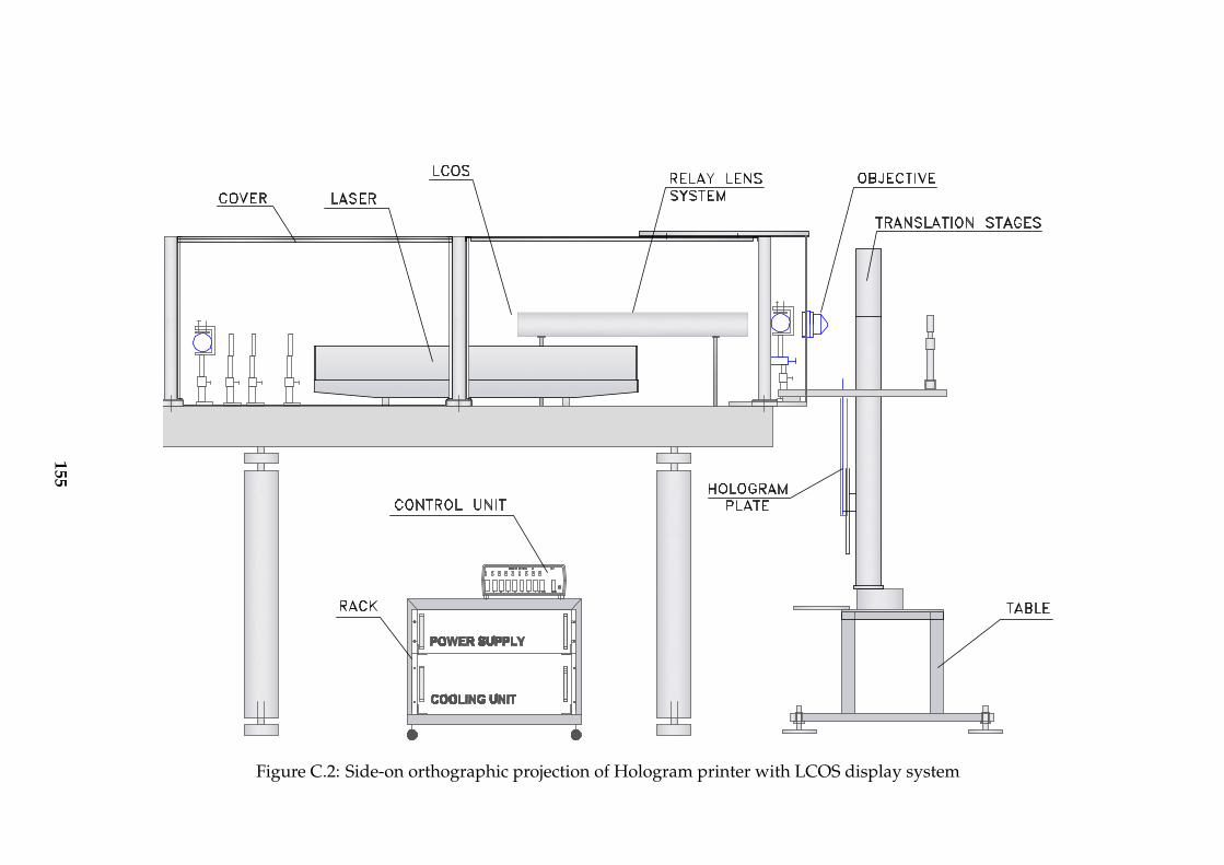
Figure C.2: Side-on orthographic projection of Hologram printer with LCOS display system
155
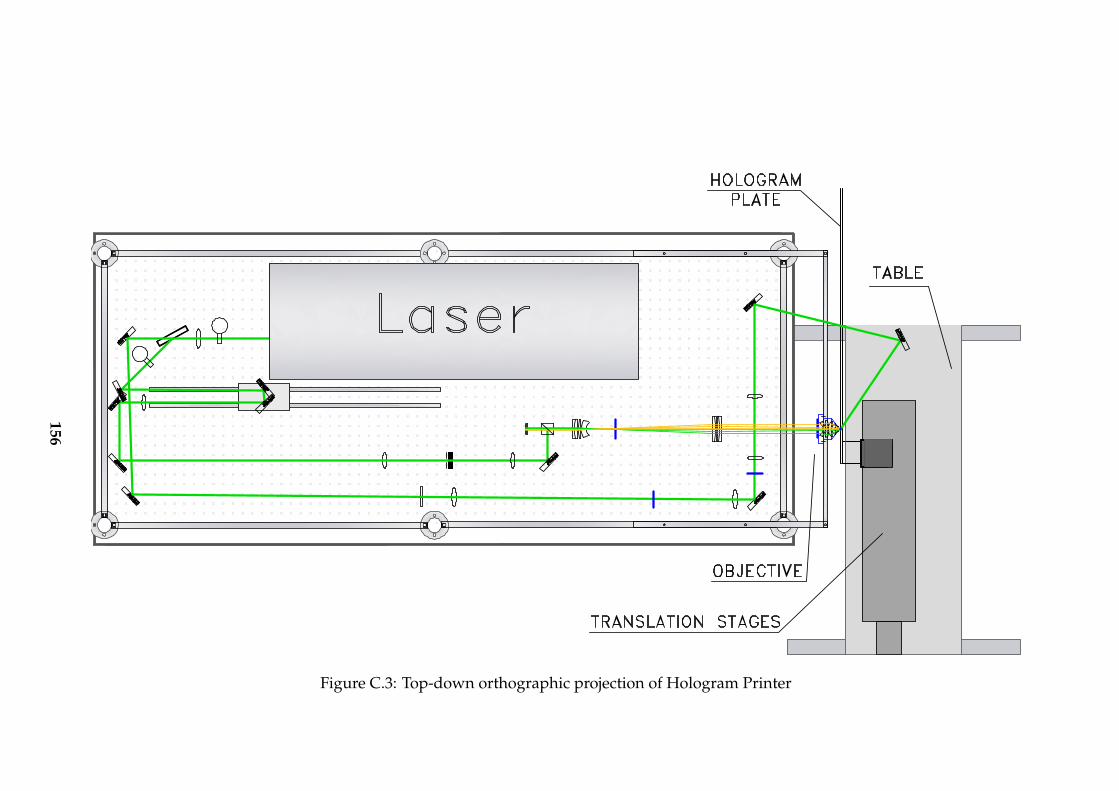
Figure C.3: Top-down orthographic projection of Hologram Printer
156

Figure C.4: Top-down orthographic projection of Hologram Printer with dimensions labelled
157

Figure C.5: Top-down orthographic projection of system to adjust optical-path distance of object beam
158
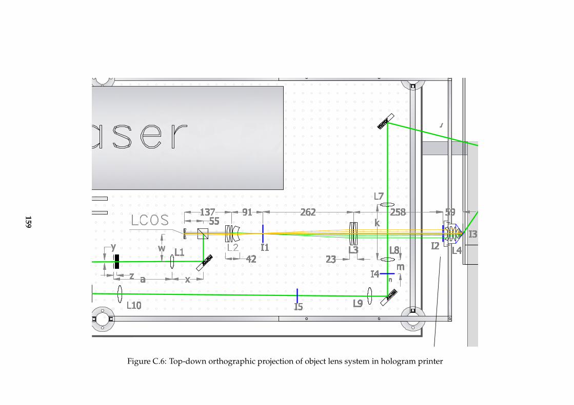
Figure C.6: Top-down orthographic projection of object lens system in hologram printer
159

DProgram listing for image analysis
Chapter 4 analysed the White Logo hologram with various techniques. Program
listing D.1 gives a matlab program for the simple analysis of a set of images. A
Guassian-blur filter is optionally applied to each image.
160

1 % Copyright (C) John Tapsell 20072 % Whether to apply a Guassian-blur3 % filter to the rendered images:4 blur_input_images=true;5
6 % Analysing all the rendered images can take a few minutes.7 % Setting this reuses the values obtained by the last run.8 reuse=false;9
10 % Read in the photograph, and convert it to grayscale.11 photo = rgb2gray(imread(’photo.png’));12
13 % Read in the closest rendered image to the photograph.14 % The photograph was taken at close to the normal angle.15 closest_match = rgb2gray(imread(’white_0360.png’));16
17 % Apply a guassian blur filter to the photograph.18 h = fspecial(’gaussian’,5,1);19 blur = imfilter(photo,h);20
21 if ~reuse22 total_intensity = 0;23 for i=0:663 % Read image white_0000.png to white_0663.png24 image_filename = [’white_’,num2str(i,’%04d’),’.png’];25 new_image = rgb2gray(imread(image_filename));26 if blur_input_images27 new_image = imfilter(new_image,h);28 end29 total_intensity=total_intensity+im2double(new_image);30 end31 end32 plot(blur(:), total_intensity(:),’.’, ’MarkerSize’, 5);
Figure D.1: Program listing for comparing the photograph of the White Logohologram and the rendered images that were used to construct the said hologram
161

EOptical fourier transform lens system
The telecentric afocal reversing lens system for the objective beam of a direct write
digital hologram printer is given below in Figures E.2, E.3 and E.4. The lens
system shown is suitable for monochromatic light of wavelength 532 nm (visible
green), entering from the polarizing beam splitter cube. The rays reflected from
the beam splitter cube are not indicated on the diagrams.
The two focal planes, I1 and I2, are also indicated1 on the diagrams.
Figure E.5 shows the lens system in in the direct-write hologram printer.
1Drawn in blue, if in color
162

Figure E.1: Lens system for imaging the Fourier transform of the LCOS (shown on the left) onto the the photosensitive emulsion,producing a holopixel (shown on the right). Figures E.2, E.3 and E.4 below provide an enlarged view. The indicated rays trace out asingle point on the LCOS display.
Figure E.2: Compound Lens L2 - First component of telecentric afocal reversing lens system. Images the Fourier transform of theLCOS plane onto the real image I2.
163

Figure E.3: Compound LensL3 – Second component oftelecentric lens system
Figure E.4: Compound Lens L4 – Fourier transforms the real image plane (I2)on the left to the holopixel plane on the right (I3)
164

Figure E.5: Top down view of design suitable for direct-write holography of reflection holograms. Sample light rays are shown for thetelescopic system. These originate parallel and spatially distinct points on the LCOS display and focus to single point with distinctangles at the final hologram plane I3. Rays below the axial ray are indicated in yellow and rays above the axial ray are indicated ingreen, for visual confirmation that the afocal lens system is indeed reversing.
165

FLCOS mechanical mount
Figure F.1 on the following page shows that the LCOS was mounted in place
with a weak corrective lens in front. This corrective lens ensures that the final
projected image has a flat focal plane. The cube split-beam polariser is mounted
in the same holder as shown. The laser light enters into the page as a plane wave
into the polariser cube. Dimension shown is in millimeters.
166
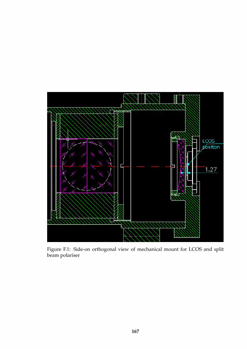
Figure F.1: Side-on orthogonal view of mechanical mount for LCOS and splitbeam polariser
167

GLens system
The parameters of the lens components in the LCOS-based hologram printer’s
relay lens system are given in Table G.1 on the next page. Each surface is given
with the material and separation distance to the next surface. All distances are
given in millimeters. Note that surfaces 14 and 21 indicate the focal image planes
I2 and I1 respectively.
168

Optical Component Values - Green Channel
Effective Focal Length = -7.669 mm
Total distance from LCOS to image plane I3 = 807.707 mm
No. Radius Clear Diameter Separation Material Lens
1 PLANE 2.301 4.00000 Air2 -20.34000 9.562 3.07000 S-SF6 L43 -9.61600 11.630 1.93000 Air L44 -7.60000 12.360 1.45000 S-SF6 L45 -26.03000 17.598 3.45000 Air L46 -25.02700 24.134 7.45000 S-SF6 L47 -16.14400 28.390 0.30000 Air L48 -201.01914 37.924 7.80000 S-SF6 L49 -35.57000 39.759 0.30000 Air L4
10 59.70000 42.100 7.03000 S-SF6 L411 1310.14201 41.384 1.27000 Air L412 27.27000 38.142 6.15000 S-SF6 L413 20.51000 32.078 14.72777 Air14 PLANE 46.000 246.59396 Air15 693.00000 64.000 4.33000 S-SF5 L316 224.90000 64.000 7.33000 S-BK7 L317 -304.80000 64.000 0.50000 Air L318 693.00000 64.000 4.33000 S-SF5 L319 224.90000 64.000 7.33000 S-BK7 L320 -304.80000 64.000 250.10000 Air21 PLANE 50.895 73.58000 Air22 -29.51000 35.980 15.20000 J-BAF7 L223 -37.10000 45.500 0.40000 Air L224 483.10001 47.000 6.40000 J-SK4 L225 -110.15000 47.000 0.20000 Air L226 129.42000 47.000 9.80000 J-SK12 L227 -80.91000 47.000 4.00000 J-SF14 L228 PLANE 47.000 50.00000 Air29 PLANE 30.000 30.00000 S-BK7 Beam cube30 PLANE 30.000 36.68504 Air31 -65.84500 30.000 2.00000 S-SF5 LCOS lens32 PLANE 30.000 1.15834 Air LCOS
Table G.1: Optical components in afocal reversing telescopic lens system usedin LCOS based hologram printer, for green channel. All distances are given inmillimeters.
169

HLaser specifications
The laser used for the digital hologram printer is a compact single oscillator flash-
lamp pumped Nd:YAG laser producing emissions in the nanosecond regime. The
laser produces TEM00 near-diffraction limited radiation at 532 nm. Single Longi-
tudinal Mode operation is provided with a built-in SLM option. Design features
include highly stable passive Q-switched linear oscillator and harmonic genera-
tion. Fundamental lasing is at 1064 nm.
170

Figure H.1: Photograph of laser, powersupply and cooling unit. Dimensionsshown in mm.
R&B Channel HV connector
Water Out
Water In
24V to Ovens
Air Temp Signal
Breadboard Heating
R&B Channel Energy Monitoring port
G Channel Energy Monitoring Port
Alignment Port
Signal to PID
G Channel Photodiode Signal
Alignment Port
Flow & HV Interlock , Shutter
R&B Channel Photodiode Signal
GroundG Channel HV Connector
Figure H.2: Labelled photograph of the laser case. Laser shown is the Red-Green-Blue but only the green channel was used for this thesis. The photodiode andheating connection wires for the temperature-feedback system can be seen.
171

Fundamenta Wavelength 1064 nmOutput Wavelength 532 nmOutput Energy 5 mJShot-to-Shot Energy Stability 3 %Pulsewidth (FHM) 50 nsBeam Divergence (1/e2) 5-7 mmBeam Divergence Near diffraction limitLinewidth < 0.002 cm−1
Repetition Rate 50 HzSpatial profile TEM00
Laser Head Size 860×360×180 mm3
Resonator Base Plate Al-alloyQ-switching PassiveFlash Tube Lifetime > 107 shotsAdvised Operating Temperature 19 - 21 ◦ CAdvised Operating Humidity < 70 % non-condensingPowering 220 V, 1 phaseWarranty Period 12 months
Table H.1: Specifications of laser used. Energy stability figure given is withtemperature-energy feedback system described in Chapter 6 on page 113.
172
IMicrolens array analysis
The following three tables give the raw data from an experiment with three dif-
ferent microlens arrays. In order to reduce speckle on the projected image, the
three different microlens arrays of were tested at different positions and the re-
sults recorded.
The mcrolens arrays are composed of thousands of small lenses (aka lenslets)
made from BK7 glass. The lenslets are spherical lenses with a radius of curvature
of the order of a millimeter. The lenslets are rectangularly packed with an aspect
ratio close or equal to that of the LCOS display system.
In the tables, ’Dist. A’ is the distance of the lens array from the closest lens
with an uncertainty of±0.1 cm. ‘Dist. B’ is the distance of the interference pattern
from the aperture with an uncertainty of ±0.5 cm, discussed in more detail in
Section 3.4 on page 51.
The important data to note in the tables is the ’Noise pattern’ column. The
173
image projected from the LCOS has speckle. This image was projected onto a
white board 1.2 m away from the final objective lens and the repeating patterns
in the speckle measured with a ruler, averaging over several. The overall contrast
of the speckle was also noted (lower is better) as well as the overall fidelity of the
image. This was judged by eye.
When the lens array focal point is imaged directly onto the LCOS, the energy
density on the LCOS is sufficiently high to risk breaking the LCOS. This was
avoided and noted in the tables were applicable.
174

I.1.FIR
ST
MIC
RO
LEN
SA
RR
AY
I.1 First microlens array
Each lenslet is rectangular with a size of 0.40 mm×0.46 mm. The lenslets are spherical lenses with a radius of 1.3 mm
Dist.A(cm)
Dist.B(cm)
Size/shape ofbeam
Average intensity acrossLCOS
Noise Pattern
1.2 8.0 Too big - too muchenergy lost
Good in the middle half,faded at edges
Very poor image - strong dominant lines of about 1-2 cm separation
3.5 5.5 Just the right size Majority is good, butfaded steps at top andbottom
On the order of a few pixels. Mediocre quality. 10big repeating structures = 14.8 cm. Very sensitive tomovement.
4.0 4.2 Just the right size Almost perfect - just slightfading at very top andbottom.
Structure at the pixel level. 10 big repeating structures= 12.5 cm
4.5 4.0 Just the right size Almost perfect - just slightfading at very top andbottom.
Structure at the pixel level. 10 big repeating structures= 12.4 cm
4.7 2.1 Just the right size Almost perfect - just slightfading at very top andbottom.
Structure at the pixel level. 10 big repeating structures= 11.1 cm. Best fidelity and low contrast image.
5.0 1.5 Just the right size Almost perfect - just slightfading at very top andbottom.
Structure at the pixel level. 10 big repeating structures= 11.5 cm
5.2 0.0 Just the right size Almost perfect - just slightfading at very top andbottom.
Structure at the pixel level. 10 big repeating structures= 10.5 cm
Continued on next page
175

I.1.FIR
ST
MIC
RO
LEN
SA
RR
AY
Raw data for first lens array continued5.5 -0.8 Just the right size Almost perfect - just slight
fading at very top andbottom.
Structure at the pixel level. 10 big repeating structures= 10.0 cm. Fidelity isn’t too bad.
5.7 -1.7 Just the right size Almost perfect -unevenness is just startingto be noticeable by eye
Structure at the pixel level. 10 big repeating structures= 10.0 cm. Fidelity isn’t too bad.
6.0 -4.0 Just the right size Almost perfect - just slightfading at very top andbottom. Unevenness is asmall bit more noticeableat top and bottom.
Structure at the pixel level. 10 big repeating structures= 9.0 cm. Fidelity isn’t too bad.
6.5 -6.8 Slightly too small Visible darkening bars attop and bottom quarters.printing. Possibly evendesirable. Softwarecorrectable.
Structure at the pixel level. 10 big repeating structures= 7.8 cm. Loosing fidelity. Possibly still okay.
7.0 < -19 Too small Much more visibledarkening bars. Dark lineson top and bottom aroundthe bars. Not suitable forholography.
Structure at the pixel level. 10 big repeating structures= 4.3 cm. Loosing fidelity. Possibly still okay.
7.5 < -19 Too small Not even at all. Looks likea spherical waffle. Notsuitable for holography.
Structure at the pixel level. 30 big repeating structures= 13.5,14.9,15.2,15.1 cm. Terrible fidelity.
8.0 < -19 Too small Not even at all. Looks likea spherical waffle. Notsuitable for holography.
Structure at the pixel level. 10 big repeating structures= 3.0 cm. Terrible fidelity.
Continued on next page
176

I.1.FIR
ST
MIC
RO
LEN
SA
RR
AY
Raw data for first lens array continued
From 7.5 cm it became more and more difficult to measure the repeating pattern.The pattern no longer repeated so obvious and was too hard to count. At 8.5 cmthe image fidelity is awful. Somewhere around 9.0 cm each lenslet focuses to apoint on the LCOS. This was not measured too accurately for fear of damagingthe LCOS. As the pixel becomes noticeably larger now and has a square shape,despite no aperture at all.
9.5 BeforeLCOS
Too small Beautifully smoothspherical Gaussian shape
Bright points were just off of focus point of eachlenslet
10.0 BeforeLCOS
Too small Beautifully smoothspherical Gaussian shape
Beautifully smooth illumination but only illuminat-ing a small middle section
Past 9.7 cm the beam becomes too large for the first lens in the lens relay telescope.This causes the energy to drop off quickly and gives a dim useless image.
Table I.1: Raw data results for first lens array. Each lenslet is rectangular with a size of 0.40 mm×0.46 mm. The lenslets are sphericallenses with a radius of 1.3 mm
177

I.2.S
EC
ON
DM
ICR
OLE
NS
AR
RAY
I.2 Second microlens array
Each lenslet is rectangular with a size of 0.20 mm×0.23 mm. The lenslets are spherical lenses with a radius of 0.65 mm. Note that the
pattern from the lens array on the projected image was much much smaller and harder to see.
Dist.A(cm)
Dist.B(cm)
Size/shape ofbeam
Average intensityacross LCOS
Noise Pattern
2.2 10.5 Just the right size Beautifully smooth.No complaints
7 big repeating structures = 25.5 cm. Worst fidelity yet.Horrible
3.0 8.0 Just the right size Beautifully smooth.No complaints
4 big repeating structures = 11.5 cm but hard to measure.Bad fidelity but getting better certainly
3.5 8.0 Just the right size Beautifully smooth.No complaints
4 big repeating structures = 10.0 cm but hard to measure.fidelity is getting a bit better but still worse then previouslensarray
4.0 7.4 Just the right size Beautifully smooth.No complaints
5 big repeating structures = 10.0 cm but hard to measure.fidelity is getting better slowly
4.5 6.4 Just the right size Beautifully smooth.No complaints
10 big repeating structures = 22.0 cm but hard to measure.fidelity is getting better slowly
5.0 5.0 Just the right size Beautifully smooth.No complaints
10 big repeating structures = 21.0 cm but hard to measure.fidelity is still getting better slowly
5.5 2.0 Just the right size Beautifully smooth.No complaints
10 big repeating structures = 19.0 cm but hard to measure.fidelity is still getting better slowly
6.0 0.0 Just the right size Beautifully smooth.No complaints
10 big repeating structures = 17.0 cm but hard to measure.fidelity is looking very nice
continued on next page..
178
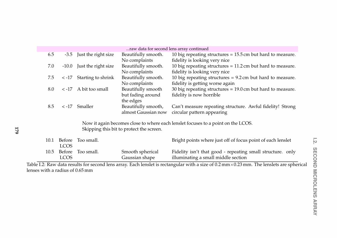
I.2.S
EC
ON
DM
ICR
OLE
NS
AR
RAY
...raw data for second lens array continued6.5 -3.5 Just the right size Beautifully smooth.
No complaints10 big repeating structures = 15.5 cm but hard to measure.fidelity is looking very nice
7.0 -10.0 Just the right size Beautifully smooth.No complaints
10 big repeating structures = 11.2 cm but hard to measure.fidelity is looking very nice
7.5 < -17 Starting to shrink Beautifully smooth.No complaints
10 big repeating structures = 9.2 cm but hard to measure.fidelity is getting worse again
8.0 < -17 A bit too small Beautifully smoothbut fading aroundthe edges
30 big repeating structures = 19.0 cm but hard to measure.fidelity is now horrible
8.5 < -17 Smaller Beautifully smooth,almost Gaussian now
Can’t measure repeating structure. Awful fidelity! Strongcircular pattern appearing
Now it again becomes close to where each lenslet focuses to a point on the LCOS.Skipping this bit to protect the screen.
10.1 BeforeLCOS
Too small. Bright points where just off of focus point of each lenslet
10.5 BeforeLCOS
Too small. Smooth sphericalGaussian shape
Fidelity isn’t that good - repeating small structure. onlyilluminating a small middle section
Table I.2: Raw data results for second lens array. Each lenslet is rectangular with a size of 0.2 mm×0.23 mm. The lenslets are sphericallenses with a radius of 0.65 mm
179

I.3.TH
IRD
MIC
RO
LEN
SA
RR
AY
I.3 Third microlens array
Each lenslet is rectangular with a size of 0.040 mm×0.046 mm. The lenslets are spherical lenses with a radius of 0.13 mm.
Dist.A(cm)
Dist.B(cm)
Size/shape ofbeam
Average intensityacross LCOS
Noise Pattern
0.0 ∼12.5 A bit too big Beautifully smooth 6 difficult to count repeating structures = 21.5 cm. Goodfidelity.
2.0 ∼10.0 Still a bit too big Beautifully smooth 6 repeating structures = 19.7 cm. Structure is slightstronger, but still good fidelity.
2.5 ∼9.5 Good Beautifully smooth 7 repeating structures = 23.6 cm. Good fidelity.3.0 ∼8.5 Good size Beautifully smooth 8 repeating structures = 25.2 cm. Good fidelity.3.5 ∼8.0 Good size Beautifully smooth 5 repeating structures = 11.4 cm. Good fidelity.4.0 ∼7.5 Good size Beautifully smooth 8 repeating structures = 18.7 cm. Good fidelity.4.5 5.5 Good size Beautifully smooth 8 repeating structures = 17.9 cm. Good fidelity.5.0 2.1 Good size Beautifully smooth 10 repeating structures = 22.0 cm. Good fidelity.5.5 0.2 A bit too small Beautifully smooth 8 repeating structures = 15.4 cm. Very nice fidelity.6.0 -1.8 3/4 Too small Some gradient
appearing5 repeating structures = 7.8 cm. Very nice fidelity.
6.5 -5.0 3/4 Too small Some gradientappearing
6 repeating structures =9.3 cm. Great fidelity.
7.0 -9.8 3/4 Too small more gradient 10 repeating structures = 12.3 cm. Great fidelity.7.5 -15.0 3/4 Too small more gradient 8 repeating structures = 8.7 cm. Great fidelity.8.0 < -17 1/2 Too small more gradient 10 repeating structures = 7.1 cm. Great fidelity.8.5 < -17 1/2 Too small unacceptable
gradient10 repeating structures = 5.0 cm. Bad fidelity because westart to see curved patterns from lens array.
continued on next page..
180
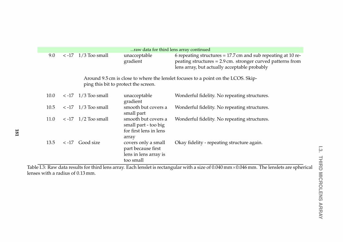
I.3.TH
IRD
MIC
RO
LEN
SA
RR
AY
...raw data for third lens array continued9.0 < -17 1/3 Too small unacceptable
gradient6 repeating structures = 17.7 cm and sub repeating at 10 re-peating structures = 2.9 cm. stronger curved patterns fromlens array, but actually acceptable probably
Around 9.5 cm is close to where the lenslet focuses to a point on the LCOS. Skip-ping this bit to protect the screen.
10.0 < -17 1/3 Too small unacceptablegradient
Wonderful fidelity. No repeating structures.
10.5 < -17 1/3 Too small smooth but covers asmall part
Wonderful fidelity. No repeating structures.
11.0 < -17 1/2 Too small smooth but covers asmall part - too bigfor first lens in lensarray
Wonderful fidelity. No repeating structures.
13.5 < -17 Good size covers only a smallpart because firstlens in lens array istoo small
Okay fidelity - repeating structure again.
Table I.3: Raw data results for third lens array. Each lenslet is rectangular with a size of 0.040 mm×0.046 mm. The lenslets are sphericallenses with a radius of 0.13 mm.
181
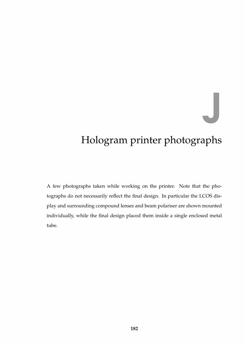
JHologram printer photographs
A few photographs taken while working on the printer. Note that the pho-
tographs do not necessarily reflect the final design. In particular the LCOS dis-
play and surrounding compound lenses and beam polariser are shown mounted
individually, while the final design placed them inside a single enclosed metal
tube.
182
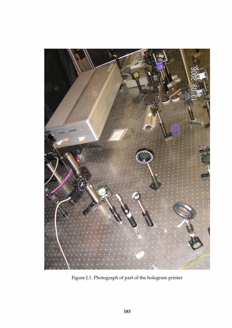
Figure J.1: Photograph of part of the hologram printer
183
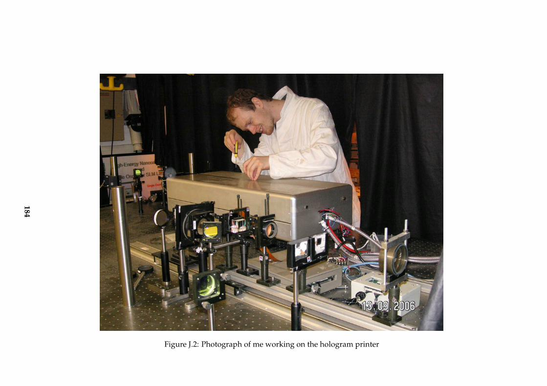
Figure J.2: Photograph of me working on the hologram printer
184

Figure J.3: Photograph of LCOS section of the hologram printer
185
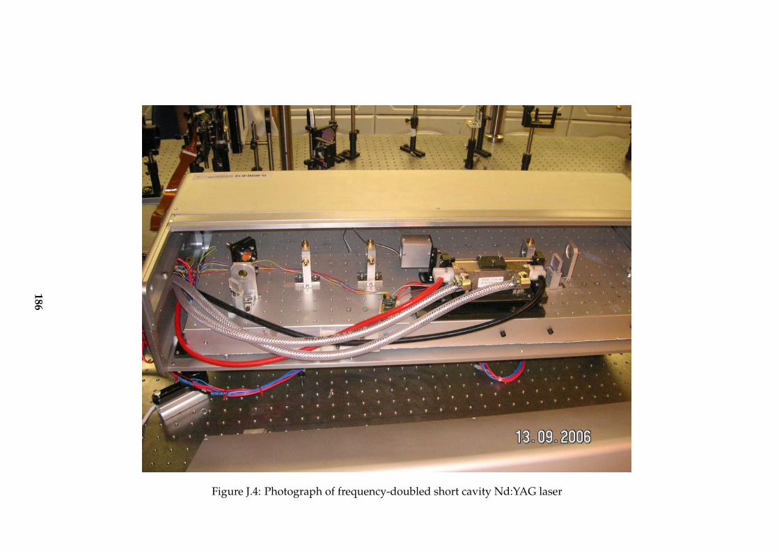
Figure J.4: Photograph of frequency-doubled short cavity Nd:YAG laser
186

![IN THE MATTER BETWEEN AUCKLAND STANDARDS CASTLES of ... · 14.5 hours for Mr Castles and 3.8 hours for Tapsell. [12] As can be seen, Mr Castles and Mr Tapsell (who was an employee,](https://img.pdfslide.us/doc/110x75/5fbe4bd8f09e6b7bfd2bf18f/in-the-matter-between-auckland-standards-castles-of-145-hours-for-mr-castles.jpg)