Embed Size (px)
Citation preview
published in Physics of Fluids, 21, 055108 (2009)
Direct simulations for wall modeling of
multicomponent reacting compressible turbulent flows
Olivier Cabrit∗
Centre Europeen de Recherche et de Formation
Avancee en Calcul Scientifique (CERFACS),
42 avenue Gaspard Coriolis,
31057 Toulouse, France
Franck Nicoud
Universite Montpellier 2,
UMR CNRS 5149 / CC51,
Place Eugene Bataillon,
34095 Montpellier, France
(Dated: May 28, 2009)
1
Abstract
A study of multicomponent reacting channel flows with significant heat transfer and low Mach
number has been performed using a set of direct and wall-resolved large eddy simulations. The
Reynolds number based on the channel half-height and the mean friction velocity is Reτ = 300 for
DNS, and Reτ = 1000 for wall-resolved LES. Two temperature ratios based on the mean centerline
temperature, Tc, and the temperature at the wall, Tw, are investigated: Tc/Tw = 1.1 for DNS,
and Tc/Tw = 3 for wall-resolved LES. The mass/momentum/energy balances are investigated,
specially showing the changes induced by multicomponent terms of the Navier-Stokes equations.
Concerning the flow dynamics, the data support the validity of the Van Driest transformation
for compressible reacting flows. Concerning heat transfer, two multicomponent terms arise in
the energy conservation balance: the laminar species diffusion which appears to be negligible in
the turbulent core, and the turbulent flux of chemical enthalpy which cannot be neglected. The
data also show that the mean composition of the mixture is at equilibrium state; a model for the
turbulent flux of chemical enthalpy is then proposed and validated. Finally, models for the total
shear stress and the total heat flux are formulated and integrated in the wall normal direction to
retrieve an analytical law-of-the-wall. This wall model is tested favorably against the DNS/LES
database.
∗Ph.D. student at Universite Montpellier 2; Electronic address: [email protected]
2
I. INTRODUCTION
In many industrial applications, the thermodynamic conditions are severe so that mo-
mentum and energy transfers are strongly coupled. Foreseeing the near wall region behavior
then becomes an issue because it is affected by the variations in fluid properties and phys-
ical effects usually not present in academic cases. For instance, the design of devices such
as piston engines or rocket-motor nozzles requires the understanding and modeling of the
multicomponent reacting compressible turbulent boundary layer. Classical wall models are
clearly not appropriate for this flow configuration and their improvement is necessary. From
a general point of view the physical effects leading to modeling issues can be listed as follows:
compressibility (generated either by strong temperature gradients or high Mach number),
wall heat transfer, streamwise pressure gradient, surface roughness, mass transfer at the wall
(associated to blowing and suction effects), buoyancy, and chemical reactions. The present
study focuses on the case when chemical reactions, wall heat transfer, and compressibility
effects are present and potentially interact. Let’s start by taking a look at a non-exhaustive
overview of the historical and theoretical bases of the present study, distinguishing works
that aim at improving the understanding of wall turbulence structure from those who deal
with its modeling.
In his pioneer work[1], Prandtl is the first one who clarified the understanding of Navier-
Stokes equations by neglecting inertia terms near the wall. He gave the name “transition
layer” to what we now call the boundary layer. Blasius[2], von Karman[3, 4], Clauser[5] and
many others extended the boundary layer theory leading their studies to the derivation of
the usual log-law formula for turbulent flows. Because this approximation is only justified
for zero pressure gradient incompressible boundary layers, the need of taking care of others
physical effects quickly arose. For instance, Patankar and Spalding[6] developed a set of
formula that aimed at accounting for the modifications induced by pressure gradient and
mass transfer through the wall. Concerning strong temperature gradients and Mach number
effects, in the 1950’s through the mid 1970’s, many experimental studies focussed on the
assessment of global quantities at the wall (friction coefficient, Nusselt number) and some
empirical correlations of engineering interest were derived[7]. In the 1980’s, the assessment
of temperature profiles has received a major advance by the work of Kader[8] who derived an
efficient correlation to account for Prandtl number effects. Despite these studies, the models
3
used in design codes for industrial applications remained simple log-law type formulations
even if some important physical effects were missing.
The compressible turbulent boundary layer with or without heat transfer is now well
documented[9–11] and the advent of direct numerical simulations (DNS)[12–15] and well-
resolved large-eddy simulations (LES)[16–20] in the 1990’s has provided reliable three-
dimensional and time-dependent data to improve the investigation of wall-bounded com-
pressible turbulent flows. Dealing with compressible effects implies to distinguish two types
of density fluctuations: 1) the first one, generally associated with low Mach number flows,
occurs from mean fluid-property variations (such as temperature or concentration); 2) the
second one arises from the compressible nature of the fluid, at high Mach number, when
significant pressure fluctuations produces density variations. Nevertheless, in the study of
wall-bounded compressible turbulent flows it is well accepted that compressibility effects are
mainly due to mean fluid-property variations[21]. This convenient assumption, referred to as
Morkovin hypothesis, allows to investigate the compressible turbulent boundary layer in the
same line of the incompressible one by paying attention to the effects of mean density vari-
ations. The use of the Van Driest transformation[22] for the modeling of compressible flows
is thus supported by this hypothesis, even at high Mach number. Experimental[23–26] and
numerical[15, 18, 27, 28] studies have shown the accuracy of the Van Driest transformation
in scaling the velocity profile with wall heat transfer and/or high Mach number flows.
The case of reacting flows where chemistry can modify the wall turbulence structure has
received little attention in the literature. Martin and Candler[29, 30] were the first, and
to the authors’s knowledge the only ones, who performed a DNS of hypersonic reacting
boundary layer. Their studies focus on the feedback mechanism between chemistry and
turbulence: exothermic reactions provide energy to the turbulent motion while the reaction
rate is increased by the turbulent temperature fluctuations. As a consequence, exothermic
reactions increase the magnitude of turbulent fluctuations while the effect of endothermic
ones appears to be the opposite. Despite this recent work, the understanding of near-wall
turbulence structure suffers from a lack of data relevant to reacting wall bounded-flows. This
is emphasized by Table I that briefly summaries the major studies available in the literature.
Reynolds Averaged Navier-Stokes (RANS) and LES methods are now widely used for the
development and design of engineering devices. Wall models are often preferred in industrial
calculations since they allow to reduce the computation demand drastically. Note also that
4
TABLE I: Non-exhaustive overview of major studies found in the literature concerning the analysis
of wall turbulence structure. References are classified according to the kind of equations implicated
in the analysis.
Velocity Velocity Velocity
- Temperature Temperature
- - Chemistry
Low Mach Kim et al.[31] Cheng & Ng[32] no reference found
number Moser et al.[33] Teitel & Antonia[34]
Hoyas et al.[35] Wang & Pletcher[18]
Jimenez et al.[36] Nicoud[28]
High Mach Huang et al.[25] Huang et al.[13] Martin & Candler[29, 30]
number Zhang et al.[26] Coleman et al.[12]
Morinishi et al.[15]
using wall models together with high-Reynolds number formulations usually leads to more
stable computations than the low Reynolds number approaches where regions with small
viscosity and stiff gradient must be handled[37]. The price to pay is the development of wall
functions for the assessment of the mass/momentum/energy fluxes at the solid boundaries
knowing the outer flow conditions at the first off-wall grid points. Note that for RANS calcu-
lations, additional prescription is necessary to insure a coherent behavior of the turbulence
model transport equations in the near wall region (the specific case of k-ǫ turbulence model
will be discussed further, in the last section of this paper).
The logarithmic structure of the overlap region of the turbulent boundary layer is now
well supported by many studies[53–56] and the classical log law is thus implemented in most
of the RANS/LES codes. It provides good results for simple incompressible flows but the
trend today is to generalize the wall function approach[42, 47, 50, 57, 58] to account for more
physics. Most of the improved models deal with streamwise pressure gradient effects[44–49],
wall roughness[42, 43], compressibility[26, 39], heat transfer[41], mass transfer[38, 39], or
even buoyancy effects[50], but a lack of data explains the poor advances made for reacting
flows (see Table II). Moreover, generalized models often make use of artificial integration
or curve-fit techniques to make the integration of equations possible[41, 50] which means
5
TABLE II: Non-exhaustive list of main references found in the literature dealing with improved wall
modeling. In this table, STG referred to strong temperature gradient, MNE to Mach number effect,
and symbols indicate whether this type of equation is discussed (•) or not (-) in the corresponding
reference.
Wall modeling issues References Model discussed
velocity temperature turbulence
Prandtl number effect Kader[8] - • -
wall mass transfer Simpson[38] • - -
Nicoud & Bradshaw[39] • - -
compressibility (STG) Subranian & Antonia[40] • • -
Han & Reitz[41] • • -
Nicoud & Bradshaw[39] • - -
Dailey et al.[19] • • -
compressibility (MNE) Huang & Coleman.[27] • • -
So et al.[26] • - -
surface roughness Shih et al.[42] • - -
Suga et al.[43] • • -
streamwise pressure gradient Huang & Bradshaw[44] • - -
Skote & Henningson[45, 46] • - -
Shih et al.[47] • - -
Nickels[48] • - -
Houra & Nagano[49] • • -
complex flows/mixed effects Craft et al.[50–52] • • •chemical reactions no reference found - - -
that they are only well suited to the applications they are derived for. It is the authors
point of view that robust and accurate models can/should be developed by simplifying and
integrating the basic flow equations. Such modeling effort must be supported by the analysis
of detailed relevant data. Classical experimental techniques cannot provide the required
space resolution for flows involving strong temperature gradients and chemical reactions.
6
An alternative is to rely on DNS and wall-resolved LES to generate precise and detailed
data set of generic turbulent flows under realistic operating conditions.
The purpose of the current paper is to extend the panel of the existing studies on in-
compressible and compressible turbulent boundary layer to the general case of wall-bounded
reacting flows. The basis of our work is a set of DNS and wall-resolved LES of low Mach
number periodic reacting channel flows with either small or large temperature gradients.
The main objectives of the present study are:
1) generate relevant reference data in the general case of multicomponent reacting com-
pressible turbulent boundary layer;
2) use this database to analyze momentum and energy balances;
3) illustrate how these balances can be used to improve the existing wall models and
account for more physics in the wall heat flux assessment.
The paper is arranged as follows. Section II presents the governing equations of reacting
flows, a short description of the numerical method, the flow parameters and the description
of the simulations. Section III provides the analysis of the mass/momentum/energy bal-
ances in order to establish the quality of the results and to underline the prevalent physical
mechanisms. Section IV illustrates how the database can be used to develop and improve
existing wall models following a generic approach. Finally, Sec. V summarizes the results of
this study.
II. EQUATIONS AND NUMERICAL STRATEGY
A. Governing equations
The conservation equations for three-dimensional, compressible, turbulent flows of react-
ing gaseous mixture are well-known and available in several text books[59, 60]. Continuity
equation (1), mass species conservation (2), momentum conservation (3), total non-chemical
energy conservation (4) and perfect gas equation of state (5) can be written with Einstein
notation (summation on i, j and l subscripted variables) in the following form:
∂ρ
∂t+
∂(ρui)
∂xi
= 0 (1)
7
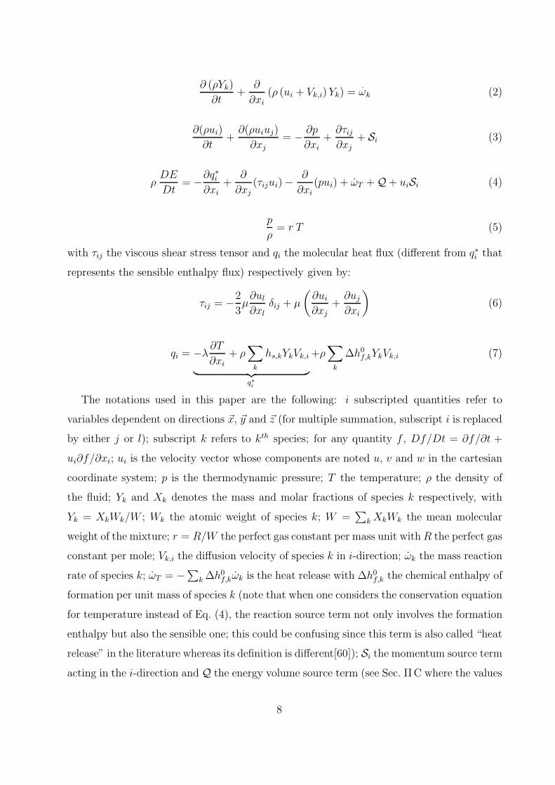
∂ (ρYk)
∂t+
∂
∂xi
(ρ (ui + Vk,i)Yk) =.ωk (2)
∂(ρui)
∂t+
∂(ρuiuj)
∂xj= − ∂p
∂xi+
∂τij
∂xj+ Si (3)
ρDE
Dt= −∂q∗i
∂xi+
∂
∂xj(τijui) −
∂
∂xi(pui) + ωT + Q + uiSi (4)
p
ρ= r T (5)
with τij the viscous shear stress tensor and qi the molecular heat flux (different from q∗i that
represents the sensible enthalpy flux) respectively given by:
τij = −2
3µ
∂ul
∂xlδij + µ
(∂ui
∂xj+
∂uj
∂xi
)(6)
qi = −λ∂T
∂xi
+ ρ∑
k
hs,kYkVk,i
︸ ︷︷ ︸q∗i
+ρ∑
k
∆h0f,kYkVk,i (7)
The notations used in this paper are the following: i subscripted quantities refer to
variables dependent on directions ~x, ~y and ~z (for multiple summation, subscript i is replaced
by either j or l); subscript k refers to kth species; for any quantity f , Df/Dt = ∂f/∂t +
ui∂f/∂xi; ui is the velocity vector whose components are noted u, v and w in the cartesian
coordinate system; p is the thermodynamic pressure; T the temperature; ρ the density of
the fluid; Yk and Xk denotes the mass and molar fractions of species k respectively, with
Yk = XkWk/W ; Wk the atomic weight of species k; W =∑
k XkWk the mean molecular
weight of the mixture; r = R/W the perfect gas constant per mass unit with R the perfect gas
constant per mole; Vk,i the diffusion velocity of species k in i-direction; ωk the mass reaction
rate of species k; ωT = −∑
k ∆h0f,kωk is the heat release with ∆h0
f,k the chemical enthalpy of
formation per unit mass of species k (note that when one considers the conservation equation
for temperature instead of Eq. (4), the reaction source term not only involves the formation
enthalpy but also the sensible one; this could be confusing since this term is also called “heat
release” in the literature whereas its definition is different[60]); Si the momentum source term
acting in the i-direction and Q the energy volume source term (see Sec. IIC where the values
8
retained for these source terms are specified); Cp,k the heat capacity at constant pressure
of species k; Cp =∑
k Cp,kYk and Cv the heat capacity at constant pressure and constant
volume of the mixture, respectively; µ and ν = µ/ρ are the dynamic and the kinematic
viscosity, respectively; λ the heat diffusion coefficient of the fluid; the possible variables to
represent enthalpy for one species are the sensible enthalpy hs,k =∫ T
T0Cp,k dT or the specific
enthalpy, hk =∫ T
T0Cp,k dT + ∆h0
f,k (sum of the sensible and the chemical parts), defined
with a reference temperature T0 = 0K for this work; the possible variables to represent
the enthalpy of the mixture are the sensible enthalpy hs =∑
k hs,kYk, the specific enthalpy
h = hs +∑
k ∆h0f,kYk, the total enthalpy ht = h + uiui/2 or the total non chemical enthalpy
H = hs + uiui/2; by analogy, es, e, et and E denote the sensible, specific, total and total
non chemical energies, respectively (one recalls that p/ρ is the difference between enthalpy
and energy, whatever the form retained is).
The derivation of the system of equations (1-7) is performed under the following assump-
tions:
• no external forces,
• effects of volume viscosity are null,
• no Dufour effect for the heat flux,
• radiation heat transfer is negligible.
The latter statement seems questionable regarding the high temperatures and strong tem-
perature variations involved in this study (see Table IV). However, the study of Amaya et
al.[61] has demonstrated that the changes introduced by the radiative source term in such
configurations do not have an incidence upon the turbulence structure of the flow. This
means that taking into account the radiative effects or not will lead to the same wall model
development. Besides, it appears that for a periodic turbulent channel flow configuration
such as case B of the present work (see Table IV and Table V), neglecting radiative heat
transfer only fathers a relative error of 7% in the prediction of the total wall heat flux.
Moreover, even if the density can vary in the computation, the buoyancy effects are
neglected for two main reasons. First, it is often necessary to separate different physical
effects in order to improve understanding of their fundamentals. Neglecting the buoyancy
effects allows us to focus on the proper density effects. Second, an estimation of the ratio
9
Gr/Re2 (Gr being the Grashof number) sustains this assumption. Indeed, with a moderate
Reynolds number (Re = 5000), a relative density ratio ∆ρ/ρw = 0.67 (maximum value
taken in the wall-resolved LES), and a kinematic viscosity of order ν ≈ 10−5 m2/s, we
find that Gr/Re2 ≈ 2630h3 (h is the reference lenght, e.g. the channel half-height in this
study). Thus, the parameter Gr/Re2 is smaller than 5% (much less than the value 0.3
advocated by Sparrow et al.[62] for the critical limit between forced convection and mixed
flows) as long as h is smaller than 0.026 meters. This means that the no-buoyancy body
force assumption is justified whether the characteristic length scale is of order 2 cm or less.
This would be a reasonable range for a true experiment, for instance based on a subscale
solid rocket motor designed to measure heat fluxes[63]. For the present simulations, this
condition is also verified as the channel half-height never exceeds 0.2 mm.
Note concerning the approximation of perfect gas equation of state
Because the mean temperature and pressure of the mixture are very high in this study
(around 3000 K and 10 MPa, respectively) the validity of the perfect gas equation of
state, Eq.(5), is also questionable. Indeed, if these operating conditions are close to the
critical point or near the pseudo-boiling line, the classical perfect gas equation of state
should be modified to take into account attractive and repulsive intermolecular forces[64].
Hence, in order to support the usability of Eq.(5), the Peng-Robinson equation of sate[65]
has been used to compute the compressibility factor, Z = PV/RT where V is the molar
volume of the mixture. As presented in Table III, Z stays very close to unity for the
three tested temperatures. This indicates that replacing Eq.(5) by a real gas equation of
state (such as the Peng-Robinson one[65]) should not have any major repercussions on the
thermodynamics of the flow. Moreover, the goal of this study is to develop a wall model
that gives reliable predictions in the most common cases (the perfect gas assumption is valid
for 95% of industrial applications); the use of a real gas equation of state is thus out of the
scope of this work.
10

TABLE III: Compressibility factor of the simulated mixture computed with the Peng-Robinson
equation of state. Results obtained for three characteristic temperatures of the present study.
Temperature(K) Compressibilityfactor
1050 K 1.02
2750 K 1.009
3000 K 1.008
B. Modeling of the transport terms
When external forces acting on the species are neglected, the exact expression of the
diffusion velocity is reduced to:
Vk,i = −∑
l
Dkl∂Xl
∂xi︸ ︷︷ ︸
mixture effect
−∑
l
Dkl(Xl − Yl)1
p
∂p
∂xi︸ ︷︷ ︸
pressure gradient effect
−∑
l
Dkl χl∂ ln T
∂xi︸ ︷︷ ︸
Soret effect
(8)
where Dkl are the multicomponent diffusion coefficients of the diffusion matrix and χl the
thermal diffusion ratio of species l. Solving the transport system Eq. (8) is an expensive
task for CFD codes and this is why the system is simplified in the present study. First of
all, the pressure gradient effect is neglected because for a periodic channel flow configuration
the pressure variations stay weak. The Soret effect is also neglected and the simplification
of Eq. (8) is achieved by the use of the Hirschfelder and Curtiss approximation[66] with cor-
rection velocity. As mentioned by Giovangigli[67] this is the best first-order accuracy model
for estimating diffusion velocities of a multicomponent mixture. It consists in replacing the
rigorous mixture effect part of the diffusion velocity system by a simpler one:
V hck,i Xk = −Dk
∂Xk
∂xi
(9)
where the V hck,i denotes the Hirschfelder and Curtiss diffusion velocity, and Dk an equiva-
lent diffusion coefficient of species k into the rest of the mixture. The latter coefficient is
built from the binary diffusion coefficients Dij which can be assessed from the gas kinetic
theory[67]:
Dk =1 − Yk∑
j 6=k Xj/Djk
(10)
Mass conservation is a specific issue when dealing with reacting flows. To insure that the
system of equations satisfies the two constraints∑
k Yk = 1 and∑
k YkVk,i = 0, a correction
11
velocity V cori is added to the Hirschfelder and Curtiss diffusion velocity V hc
k,i . At each time
step, the correction velocity is computed as:
V cori =
∑
k
DkWk
W
∂Xk
∂xi
(11)
so that the diffusion velocities for each species k:
Vk,i = V hck,i + V cor
i (12)
satisfy the constrain∑
k YkVk,i = 0. Combined with the assumption of constant Schmidt
numbers, the Hirschfelder and Curtiss approximation is very convenient because the equiv-
alent diffusion coefficients can be easily related to the kinematic viscosity according to:
Dk = ν/Sck. The problem is then efficiently closed by imposing the Schmidt numbers and it
is not necessary to compute the Dij coefficients which are complex functions of collision in-
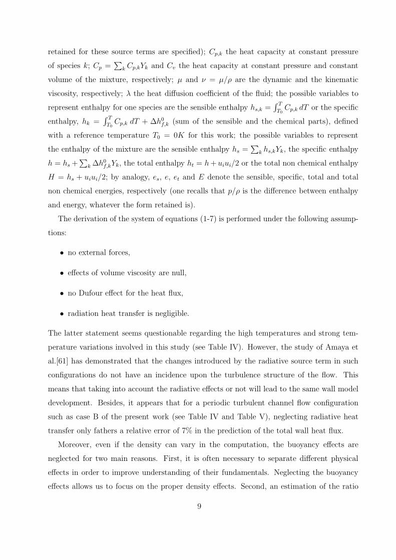
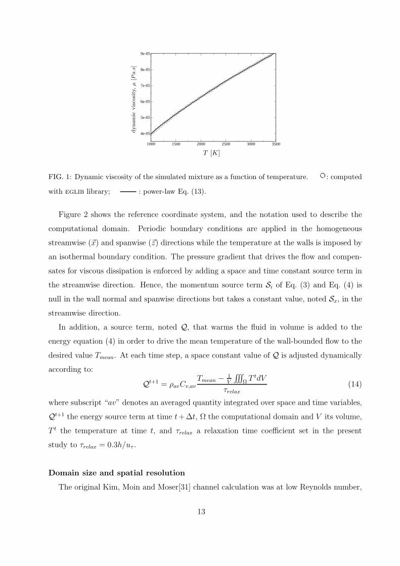
tegrals and thermodynamics variables. Note that in the present work, the dynamic viscosity
is modeled by a power-law expression:
µ = µref
(T
Tref
)c
(13)
where µref = 8.194 × 10⁻⁵ Pa.s, Tref = 3000 K and c = 0.656. This choice is supported
by Fig. 1 that presents the difference between the retained model and the dynamic viscosity
of the simulated mixture computed with eglib library[68, 69]. This plot argues that a
Sutherland type formulation is not necessary for the temperature range covered in this
study.
C. Set up of the simulations
In order to cover different kinds of turbulent wall-bounded flows and to isolate some
physical processes such as chemical reactions or strong temperature gradients, four different
periodic channel flows have been computed. Their physical characteristics are summarized
in Table IV in which Reτ is the target friction Reynolds number, Rec the Reynolds number
based on the channel half-height (denoted by h in this paper) and centerline properties, and
Reb the Reynolds number based on bulk quantities (i.e. the bulk density ρb = 1/h∫ h
0ρ dy,
bulk velocity ub = 1/h∫ h
0ρu dy/ρb, and viscosity at the wall). Note that case A is the
reference case for this study because this is the one that includes less physical effects: the
temperature gradient is small and no chemical reaction is activated.
12
1000 1500 2000 2500 3000 3500
4e-05
5e-05
6e-05
7e-05
8e-05
9e-05
dynam
icvis
cosi
ty,µ
[Pa.s
]
T [K]
FIG. 1: Dynamic viscosity of the simulated mixture as a function of temperature. E: computed
with eglib library; : power-law Eq. (13).
Figure 2 shows the reference coordinate system, and the notation used to describe the
computational domain. Periodic boundary conditions are applied in the homogeneous
streamwise (~x) and spanwise (~z) directions while the temperature at the walls is imposed by
an isothermal boundary condition. The pressure gradient that drives the flow and compen-
sates for viscous dissipation is enforced by adding a space and time constant source term in
the streamwise direction. Hence, the momentum source term Si of Eq. (3) and Eq. (4) is
null in the wall normal and spanwise directions but takes a constant value, noted Sx, in the
streamwise direction.
In addition, a source term, noted Q, that warms the fluid in volume is added to the
energy equation (4) in order to drive the mean temperature of the wall-bounded flow to the
desired value Tmean. At each time step, a space constant value of Q is adjusted dynamically
according to:
Qt+1 = ρavCv,av
Tmean − 1V
∫∫∫Ω
T tdV
τrelax(14)
where subscript “av” denotes an averaged quantity integrated over space and time variables,
Qt+1 the energy source term at time t+∆t, Ω the computational domain and V its volume,
T t the temperature at time t, and τrelax a relaxation time coefficient set in the present
study to τrelax = 0.3h/uτ .
Domain size and spatial resolution
The original Kim, Moin and Moser[31] channel calculation was at low Reynolds number,
13
y
xz
flow
Lz
Lx
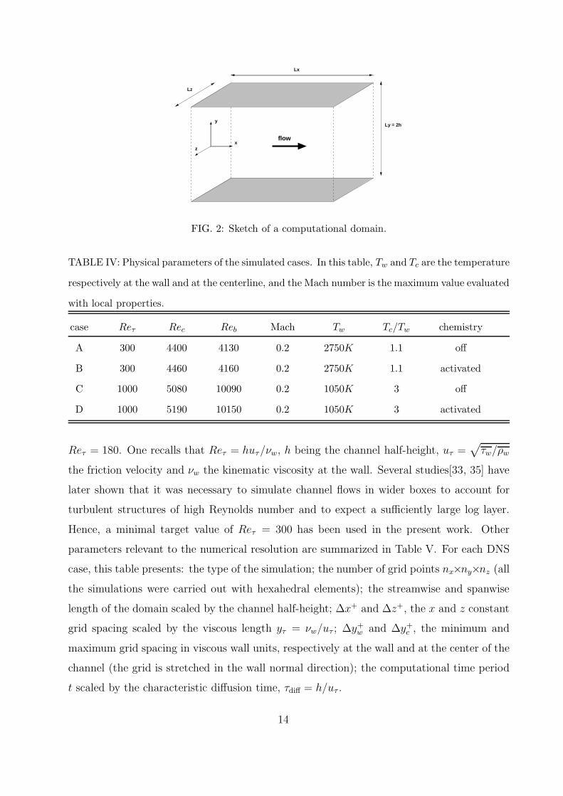
Ly = 2h
FIG. 2: Sketch of a computational domain.
TABLE IV: Physical parameters of the simulated cases. In this table, Tw and Tc are the temperature
respectively at the wall and at the centerline, and the Mach number is the maximum value evaluated
with local properties.
case Reτ Rec Reb Mach Tw Tc/Tw chemistry
A 300 4400 4130 0.2 2750K 1.1 off
B 300 4460 4160 0.2 2750K 1.1 activated
C 1000 5080 10090 0.2 1050K 3 off
D 1000 5190 10150 0.2 1050K 3 activated
Reτ = 180. One recalls that Reτ = huτ/νw, h being the channel half-height, uτ =√
τw/ρw
the friction velocity and νw the kinematic viscosity at the wall. Several studies[33, 35] have
later shown that it was necessary to simulate channel flows in wider boxes to account for
turbulent structures of high Reynolds number and to expect a sufficiently large log layer.
Hence, a minimal target value of Reτ = 300 has been used in the present work. Other
parameters relevant to the numerical resolution are summarized in Table V. For each DNS
case, this table presents: the type of the simulation; the number of grid points nx×ny×nz (all
the simulations were carried out with hexahedral elements); the streamwise and spanwise
length of the domain scaled by the channel half-height; ∆x+ and ∆z+, the x and z constant
grid spacing scaled by the viscous length yτ = νw/uτ ; ∆y+w and ∆y+
c , the minimum and
maximum grid spacing in viscous wall units, respectively at the wall and at the center of the
channel (the grid is stretched in the wall normal direction); the computational time period
t scaled by the characteristic diffusion time, τdiff = h/uτ .
14
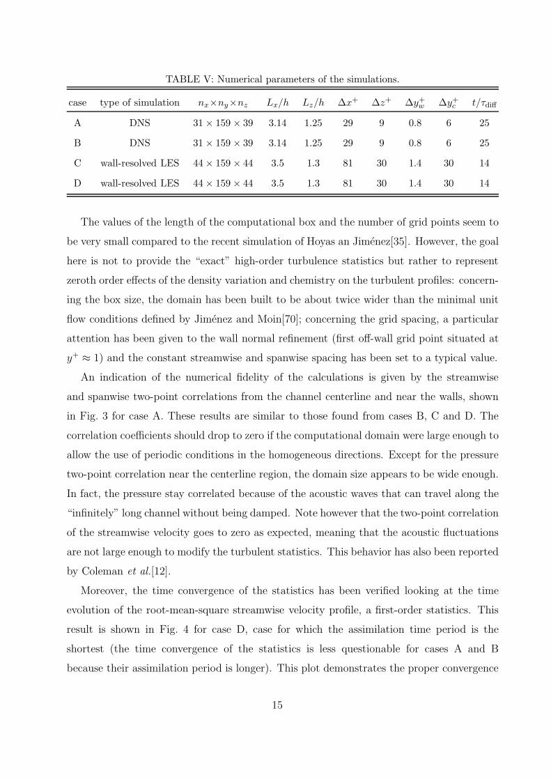
TABLE V: Numerical parameters of the simulations.
case type of simulation nx×ny×nz Lx/h Lz/h ∆x+ ∆z+ ∆y+w ∆y+
c t/τdiff
A DNS 31 × 159 × 39 3.14 1.25 29 9 0.8 6 25
B DNS 31 × 159 × 39 3.14 1.25 29 9 0.8 6 25
C wall-resolved LES 44 × 159 × 44 3.5 1.3 81 30 1.4 30 14
D wall-resolved LES 44 × 159 × 44 3.5 1.3 81 30 1.4 30 14
The values of the length of the computational box and the number of grid points seem to
be very small compared to the recent simulation of Hoyas an Jimenez[35]. However, the goal
here is not to provide the “exact” high-order turbulence statistics but rather to represent
zeroth order effects of the density variation and chemistry on the turbulent profiles: concern-
ing the box size, the domain has been built to be about twice wider than the minimal unit
flow conditions defined by Jimenez and Moin[70]; concerning the grid spacing, a particular
attention has been given to the wall normal refinement (first off-wall grid point situated at
y+ ≈ 1) and the constant streamwise and spanwise spacing has been set to a typical value.
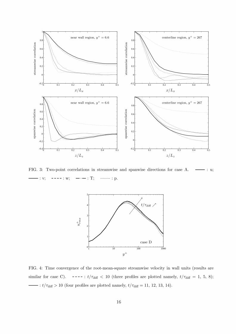
An indication of the numerical fidelity of the calculations is given by the streamwise
and spanwise two-point correlations from the channel centerline and near the walls, shown
in Fig. 3 for case A. These results are similar to those found from cases B, C and D. The
correlation coefficients should drop to zero if the computational domain were large enough to
allow the use of periodic conditions in the homogeneous directions. Except for the pressure
two-point correlation near the centerline region, the domain size appears to be wide enough.
In fact, the pressure stay correlated because of the acoustic waves that can travel along the
“infinitely” long channel without being damped. Note however that the two-point correlation
of the streamwise velocity goes to zero as expected, meaning that the acoustic fluctuations
are not large enough to modify the turbulent statistics. This behavior has also been reported
by Coleman et al.[12].
Moreover, the time convergence of the statistics has been verified looking at the time
evolution of the root-mean-square streamwise velocity profile, a first-order statistics. This
result is shown in Fig. 4 for case D, case for which the assimilation time period is the
shortest (the time convergence of the statistics is less questionable for cases A and B
because their assimilation period is longer). This plot demonstrates the proper convergence
15
0 0.1 0.2 0.3 0.4 0.5-0.2
0
0.2
0.4
0.6
0.8
1st
ream
wis
eco
rrel
ation
x/Lx
near wall region, y+ = 6.6
0 0.1 0.2 0.3 0.4 0.5-0.2
0
0.2
0.4
0.6
0.8
stre
am
wis
eco
rrel
ation
x/Lx
centerline region, y+ = 267
0 0.1 0.2 0.3 0.4 0.5-0.4
-0.2
0
0.2
0.4
0.6
0.8
1
spanw
ise
corr
elation
z/Lz
near wall region, y+ = 6.6
0 0.1 0.2 0.3 0.4 0.5-0.2
0
0.2
0.4
0.6
0.8
spanw
ise
corr
elation
z/Lz
centerline region, y+ = 267
FIG. 3: Two-point correlations in streamwise and spanwise directions for case A. : u;
: v; : w; : T; ········ : p.
1 10 100 10000
1
2
3
4
5
t/τdiff ր
case D
y+
u+ rm
s
FIG. 4: Time convergence of the root-mean-square streamwise velocity in wall units (results are
similar for case C). : t/τdiff < 10 (three profiles are plotted namely, t/τdiff = 1, 5, 8);
: t/τdiff > 10 (four profiles are plotted namely, t/τdiff = 11, 12, 13, 14).
16
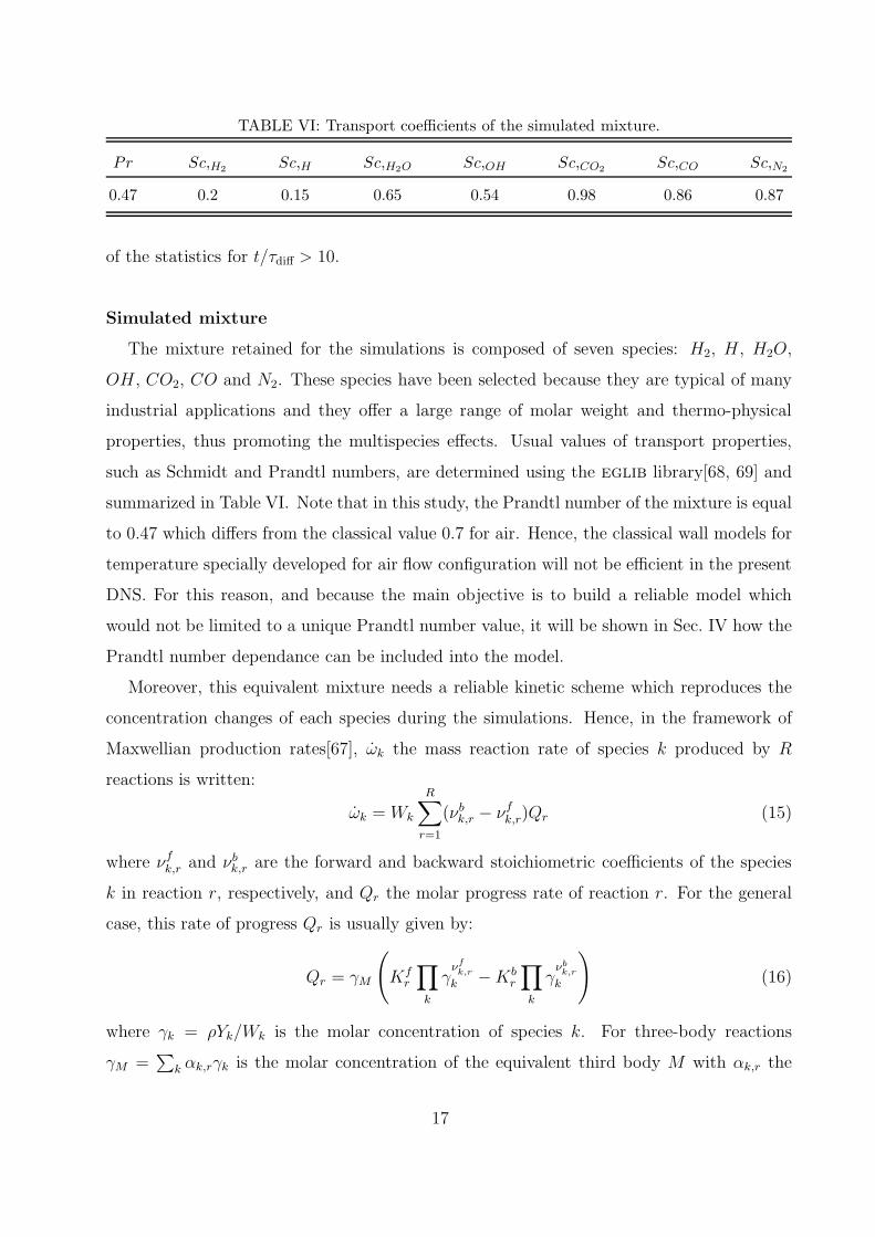
TABLE VI: Transport coefficients of the simulated mixture.
Pr Sc,H2Sc,H Sc,H2O Sc,OH Sc,CO2
Sc,CO Sc,N2
0.47 0.2 0.15 0.65 0.54 0.98 0.86 0.87
of the statistics for t/τdiff > 10.
Simulated mixture
The mixture retained for the simulations is composed of seven species: H2, H , H2O,
OH , CO2, CO and N2. These species have been selected because they are typical of many
industrial applications and they offer a large range of molar weight and thermo-physical
properties, thus promoting the multispecies effects. Usual values of transport properties,
such as Schmidt and Prandtl numbers, are determined using the eglib library[68, 69] and
summarized in Table VI. Note that in this study, the Prandtl number of the mixture is equal
to 0.47 which differs from the classical value 0.7 for air. Hence, the classical wall models for
temperature specially developed for air flow configuration will not be efficient in the present
DNS. For this reason, and because the main objective is to build a reliable model which
would not be limited to a unique Prandtl number value, it will be shown in Sec. IV how the
Prandtl number dependance can be included into the model.
Moreover, this equivalent mixture needs a reliable kinetic scheme which reproduces the
concentration changes of each species during the simulations. Hence, in the framework of
Maxwellian production rates[67], ωk the mass reaction rate of species k produced by R
reactions is written:
ωk = Wk
R∑
r=1
(νbk,r − νf
k,r)Qr (15)
where νfk,r and νb
k,r are the forward and backward stoichiometric coefficients of the species
k in reaction r, respectively, and Qr the molar progress rate of reaction r. For the general
case, this rate of progress Qr is usually given by:
Qr = γM
(Kf
r
∏
k
γνf
k,r
k − Kbr
∏
k
γνb
k,r
k
)(16)
where γk = ρYk/Wk is the molar concentration of species k. For three-body reactions
γM =∑
k αk,rγk is the molar concentration of the equivalent third body M with αk,r the
17
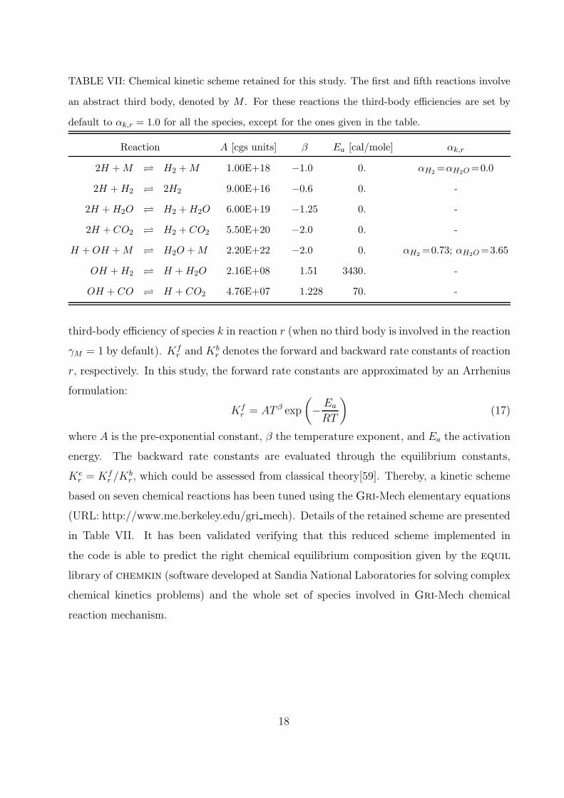
TABLE VII: Chemical kinetic scheme retained for this study. The first and fifth reactions involve
an abstract third body, denoted by M . For these reactions the third-body efficiencies are set by
default to αk,r = 1.0 for all the species, except for the ones given in the table.
Reaction A [cgs units] β Ea [cal/mole] αk,r
2H + M H2 + M 1.00E+18 −1.0 0. αH2=αH2O =0.0
2H + H2 2H2 9.00E+16 −0.6 0. -
2H + H2O H2 + H2O 6.00E+19 −1.25 0. -
2H + CO2 H2 + CO2 5.50E+20 −2.0 0. -
H + OH + M H2O + M 2.20E+22 −2.0 0. αH2=0.73; αH2O =3.65
OH + H2 H + H2O 2.16E+08 1.51 3430. -
OH + CO H + CO2 4.76E+07 1.228 70. -
third-body efficiency of species k in reaction r (when no third body is involved in the reaction
γM = 1 by default). Kfr and Kb
r denotes the forward and backward rate constants of reaction
r, respectively. In this study, the forward rate constants are approximated by an Arrhenius
formulation:
Kfr = AT β exp
(− Ea
RT
)(17)
where A is the pre-exponential constant, β the temperature exponent, and Ea the activation
energy. The backward rate constants are evaluated through the equilibrium constants,
Ker = Kf
r /Kbr , which could be assessed from classical theory[59]. Thereby, a kinetic scheme
based on seven chemical reactions has been tuned using the Gri-Mech elementary equations
(URL: http://www.me.berkeley.edu/gri mech). Details of the retained scheme are presented
in Table VII. It has been validated verifying that this reduced scheme implemented in
the code is able to predict the right chemical equilibrium composition given by the equil
library of chemkin (software developed at Sandia National Laboratories for solving complex
chemical kinetics problems) and the whole set of species involved in Gri-Mech chemical
reaction mechanism.
18
D. Numerical solver
DNS/LES were performed with the AVBP solver developed at CERFACS. This parallel
code offers the capability to handle unstructured or structured grids in order to solve the
full 3D compressible reacting Navier-Stokes equations with a cell-vertex formulation. During
the past years, its efficiency and accuracy have been widely demonstrated in both LES and
DNS for different flow configurations[71–73].
A centered Galerkin finite element method with a three-step Runge-Kutta temporal in-
tegration method has been used in the present study to solve the flow equations described
above. This numerical scheme is fourth order accurate in space, third order accurate in
time, and thus compatible with the grid resolution used (see Table V) to provide reliable
statistics of the flow. The efficiency of this numerical method has been successfully tested
by Colin & Rudgyard[74].
Finally, the subgrid-scale stress model applied for wall-resolved LES is the WALE (Wall-
Adapting Local Eddy-viscosity) model[75] specially developed for this kind of wall-bounded
flows. It is notably able to recover the proper y3 damping scaling for eddy viscosity at the
wall.
III. DNS RESULTS
The forthcoming sections present the profiles obtained after a statistical treatment has
been applied to the simulation results. It consists in performing averages over the homoge-
neous directions (~x and ~z) and time (the integration time is given in Table V). This averaging
process implies that any partial derivative of a variable f in the wall normal direction is
equivalent to a total derivative, i.e. ∂f/∂y ≡ df/dy. Let us introduce the notations used
in the equations that follow: either · or 〈 · 〉 for the ensemble average; either · or · for
the Favre average defined for a variable f as f = 〈ρf〉/〈ρ〉 ; the single prime, ′, and the
double prime, ′′, represent the turbulent fluctuations with respect to Reynolds and Favre
averages respectively.
A wall model allows to predict wall quantities such as the shear stress, τw, and the heat
flux, qw, from the knowledge of the flow quantities far from the wall. Typically, these two
parameters are functions of velocity and temperature but in the context of multicomponent
19
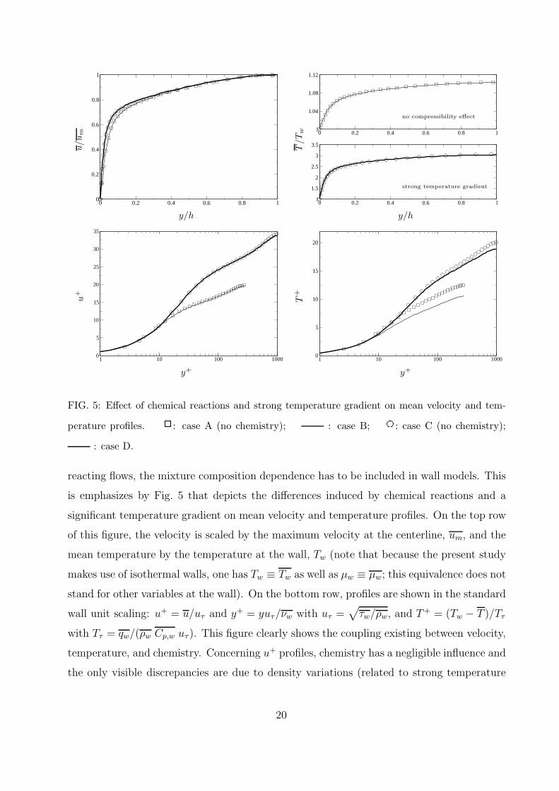
0 0.2 0.4 0.6 0.8 10
0.2
0.4
0.6
0.8
1
y/h
u/u
m 0 0.2 0.4 0.6 0.8 11
1.04
1.08
1.12
0 0.2 0.4 0.6 0.8 11
1.5
2
2.5
3
3.5
y/h
T/T
w
no compressibility effect
strong temperature gradient
1 10 100 10000
5
10
15
20
25
30
35
y+
u+
1 10 100 10000
5
10
15
20
y+
T+
FIG. 5: Effect of chemical reactions and strong temperature gradient on mean velocity and tem-
perature profiles. : case A (no chemistry); : case B; E: case C (no chemistry);
: case D.
reacting flows, the mixture composition dependence has to be included in wall models. This
is emphasizes by Fig. 5 that depicts the differences induced by chemical reactions and a
significant temperature gradient on mean velocity and temperature profiles. On the top row
of this figure, the velocity is scaled by the maximum velocity at the centerline, um, and the
mean temperature by the temperature at the wall, Tw (note that because the present study
makes use of isothermal walls, one has Tw ≡ Tw as well as µw ≡ µw; this equivalence does not
stand for other variables at the wall). On the bottom row, profiles are shown in the standard
wall unit scaling: u+ = u/uτ and y+ = yuτ/νw with uτ =√
τw/ρw, and T+ = (Tw − T )/Tτ
with Tτ = qw/(ρw Cp,w uτ ). This figure clearly shows the coupling existing between velocity,
temperature, and chemistry. Concerning u+ profiles, chemistry has a negligible influence and
the only visible discrepancies are due to density variations (related to strong temperature
20
gradient). Concerning T+ profiles (representing the temperature profile scaled by the wall
heat flux), the discrepancies observed for the four simulated cases indicate that the wall heat
flux is both sensitive to chemistry and strong temperature gradient, and that none of these
two effects can be neglected compared to the other one. In others words, even if chemical
reactions do not seem to have an influence on the mean velocity and temperatures profiles
(top row of Fig. 5), they actually have an important effect on the fluxes at the wall. This
justifies the need of taking care of fluid heterogeneity in wall models. Hence, the coupled
wall functions derived should have the form of a system of two equations τw = τw(u, T, Yk)
and qw = qw(u, T, Yk).
First of all, the quality of the simulations and the efficiency of the averaging procedure
will be tested by verifying that the balance of each conservation equation is well closed.
The study of species mass fraction/momentum/energy balances will then help in under-
standing the behavior of reacting compressible turbulent wall-bounded flows, investigating
which terms could be neglected in the turbulent momentum/energy transfers for developing
a new wall model. For clarity reasons and because this study mostly focusses on multi-
component/chemistry effects, results from cases B and D will be mainly shown in what
follows.
A. Species mass fraction balances
The averaging procedure for equation (2) leads to the following expression:
d(ρ vYk
)
dy+
d(ρ Vk,yYk
)
dy= ωk (18)
where the first left hand side (LHS) term can be assimilated to the divergence of the convec-
tive velocity field associated to species k, the second one to the divergence of the diffusion
velocity field for the kth species and the right hand side (RHS) term to the mean production
rate of species k. Figure 6 compares the influence of LHS and RHS terms of Eq. (18) for
each species. The balances are well closed which indicates that the simulation is sufficiently
time-converged and that the averaging time is long enough to proceed to an analysis of these
balances (the maximum closure error is around 5% at the wall for species OH). Another
good criterion to validate the quality of the DNS and of its post-processing is to check that
the condition v = 0, resulting from the continuity equation (1) and the no-slip condition at
21
0.01 0.1 1-1500
-1000
-500
0
500
y/h
h
kg·m
−3·s−
1i
H
0.01 0.1 1-500
0
500
1000
1500
y/h
h
kg·m
−3·s−
1i
H2
0.01 0.1 1-1500
-1000
-500
0
500
1000
y/h
h
kg·m
−3·s−
1i
H2O
0.01 0.1 1-1000
-800
-600
-400
-200
0
200
400
y/h
h
kg·m
−3·s−
1i
OH
0.01 0.1 1-3000
-2000
-1000
0
1000
2000
y/h
h
kg·m
−3·s−
1i
CO
0.01 0.1 1-1000
0
1000
2000
3000
4000
y/h
h
kg·m
−3·s−
1i
CO2
0.01 0.1 1-4000
-3000
-2000
-1000
0
1000
2000
3000
4000
y/h
h
kg·m
−3·s−
1i
N2
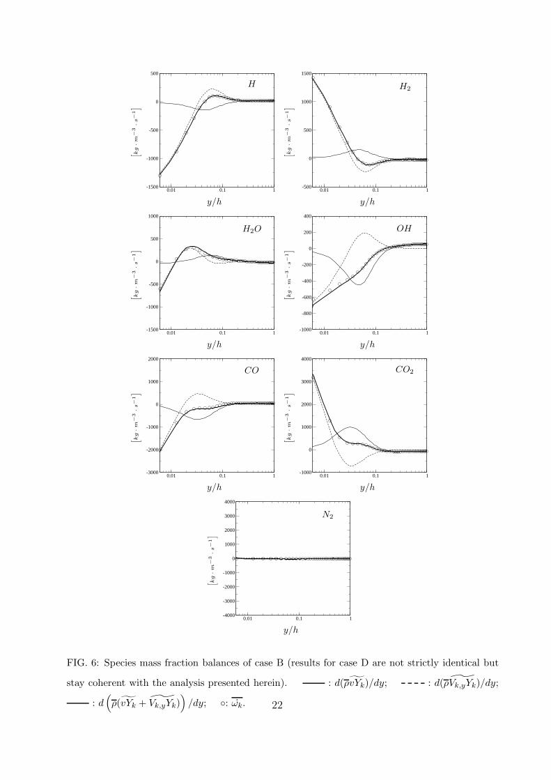
FIG. 6: Species mass fraction balances of case B (results for case D are not strictly identical but
stay coherent with the analysis presented herein). : d(ρvYk)/dy; : d(ρVk,yYk)/dy;
: d(ρ(vYk + Vk,yYk)
)/dy; : ωk. 22
0 0.2 0.4 0.6 0.8 1-7×10⁻³
-6×10⁻³
-5×10⁻³
-4×10⁻³
-3×10⁻³
-2×10⁻³
-1×10⁻³
0
y/h
wall
norm
alvel
oci
ty
case B
0 0.2 0.4 0.6 0.8 1-7×10⁻²
-6×10⁻²
-5×10⁻²
-4×10⁻²
-3×10⁻²
-2×10⁻²
-1×10⁻²
0
y/h
wall
norm
alvel
oci
ty
case D
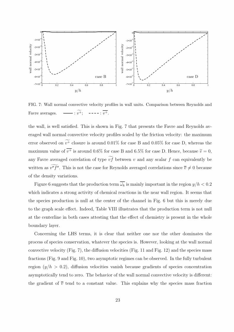
FIG. 7: Wall normal convective velocity profiles in wall units. Comparison between Reynolds and
Favre averages. : v+; : v+.
the wall, is well satisfied. This is shown in Fig. 7 that presents the Favre and Reynolds av-
eraged wall normal convective velocity profiles scaled by the friction velocity: the maximum
error observed on v+ closure is around 0.01% for case B and 0.05% for case D, whereas the
maximum value of v+ is around 0.6% for case B and 6.5% for case D. Hence, because v = 0,
any Favre averaged correlation of type vf between v and any scalar f can equivalently be
written as v′′f ′′. This is not the case for Reynolds averaged correlations since v 6= 0 because
of the density variations.
Figure 6 suggests that the production term ωk is mainly important in the region y/h < 0.2
which indicates a strong activity of chemical reactions in the near wall region. It seems that
the species production is null at the center of the channel in Fig. 6 but this is merely due
to the graph scale effect. Indeed, Table VIII illustrates that the production term is not null
at the centerline in both cases attesting that the effect of chemistry is present in the whole
boundary layer.
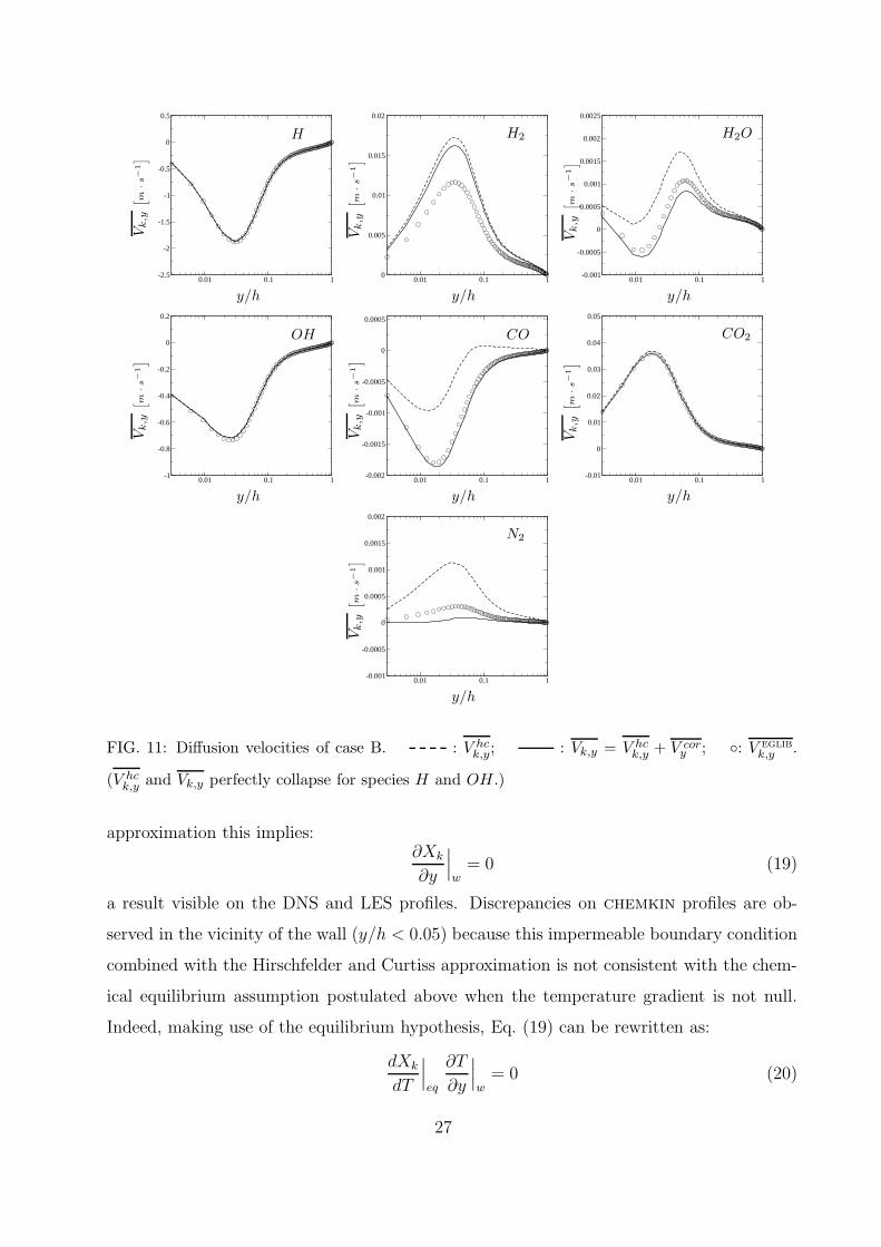
Concerning the LHS terms, it is clear that neither one nor the other dominates the
process of species conservation, whatever the species is. However, looking at the wall normal
convective velocity (Fig. 7), the diffusion velocities (Fig. 11 and Fig. 12) and the species mass
fractions (Fig. 9 and Fig. 10), two asymptotic regimes can be observed. In the fully turbulent
region (y/h > 0.2), diffusion velocities vanish because gradients of species concentration
asymptotically tend to zero. The behavior of the wall normal convective velocity is different:
the gradient of v tend to a constant value. This explains why the species mass fraction
23
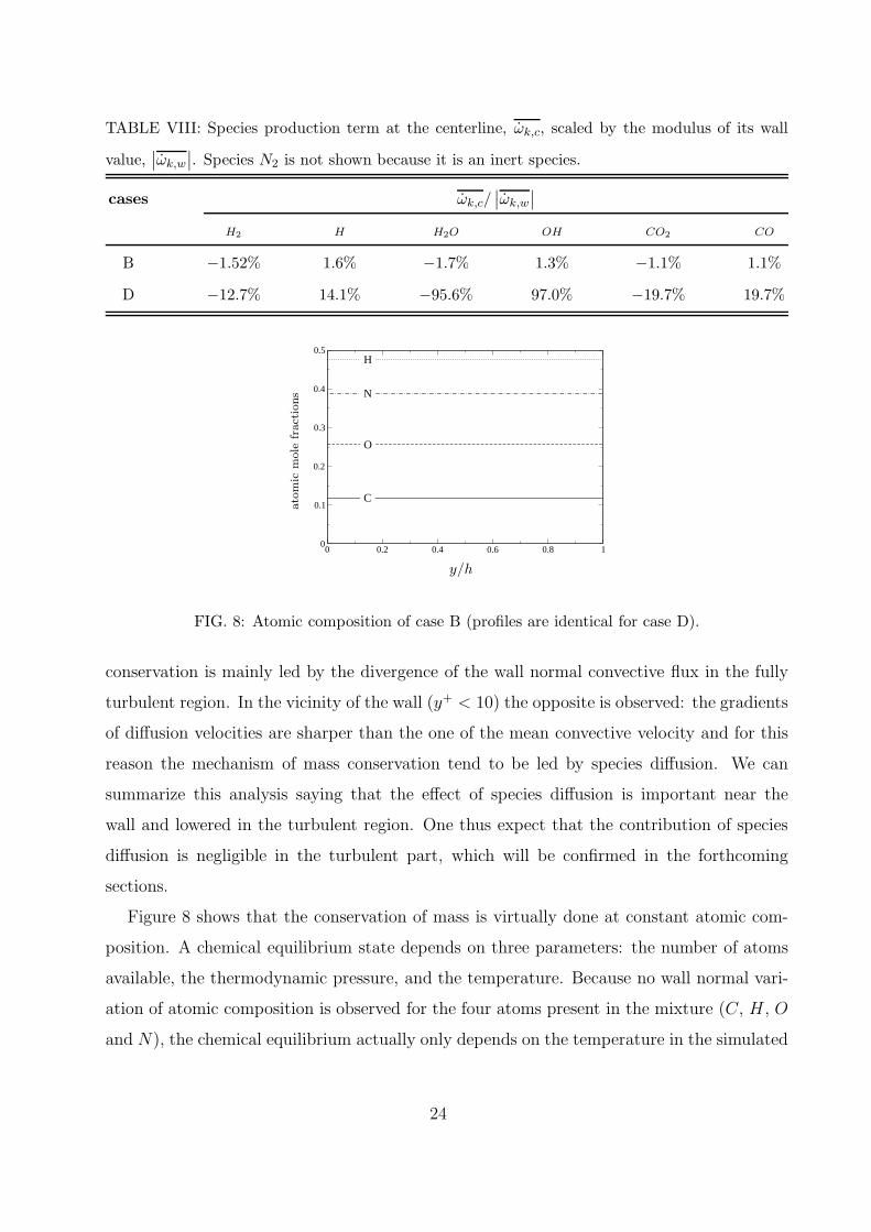
TABLE VIII: Species production term at the centerline, ωk,c, scaled by the modulus of its wall
value,∣∣ωk,w
∣∣. Species N2 is not shown because it is an inert species.
cases ωk,c/∣∣ωk,w
∣∣
H2 H H2O OH CO2 CO
B −1.52% 1.6% −1.7% 1.3% −1.1% 1.1%
D −12.7% 14.1% −95.6% 97.0% −19.7% 19.7%
0 0.2 0.4 0.6 0.8 10
0.1
0.2
0.3
0.4
0.5H
N
O
C
y/h
ato
mic
mole
fract
ions
FIG. 8: Atomic composition of case B (profiles are identical for case D).
conservation is mainly led by the divergence of the wall normal convective flux in the fully
turbulent region. In the vicinity of the wall (y+ < 10) the opposite is observed: the gradients
of diffusion velocities are sharper than the one of the mean convective velocity and for this
reason the mechanism of mass conservation tend to be led by species diffusion. We can
summarize this analysis saying that the effect of species diffusion is important near the
wall and lowered in the turbulent region. One thus expect that the contribution of species
diffusion is negligible in the turbulent part, which will be confirmed in the forthcoming
sections.
Figure 8 shows that the conservation of mass is virtually done at constant atomic com-
position. A chemical equilibrium state depends on three parameters: the number of atoms
available, the thermodynamic pressure, and the temperature. Because no wall normal vari-
ation of atomic composition is observed for the four atoms present in the mixture (C, H , O
and N), the chemical equilibrium actually only depends on the temperature in the simulated
24
0 0.2 0.4 0.6 0.8 10.0002
0.0003
0.0004
0.0005
0.0006
y/h
Yk
H
0 0.2 0.4 0.6 0.8 10.0391
0.0392
0.0393
0.0394
0.0395
y/h
Yk
H2
0 0.2 0.4 0.6 0.8 10.12640
0.12645
0.12650
0.12655
0.12660
0.12665
0.12670
y/h
Yk
H2O
0 0.2 0.4 0.6 0.8 10.0000
0.0005
0.0010
0.0015
0.0020
y/h
Yk
OH
0 0.2 0.4 0.6 0.8 10.3770
0.3775
0.3780
0.3785
0.3790
0.3795
0.3800
y/h
Yk
CO
0 0.2 0.4 0.6 0.8 10.0290
0.0295
0.0300
0.0305
0.0310
0.0315
0.0320
y/h
Yk
CO2
0 0.2 0.4 0.6 0.8 10.422
0.423
0.424
0.425
0.426
y/h
Yk
N2
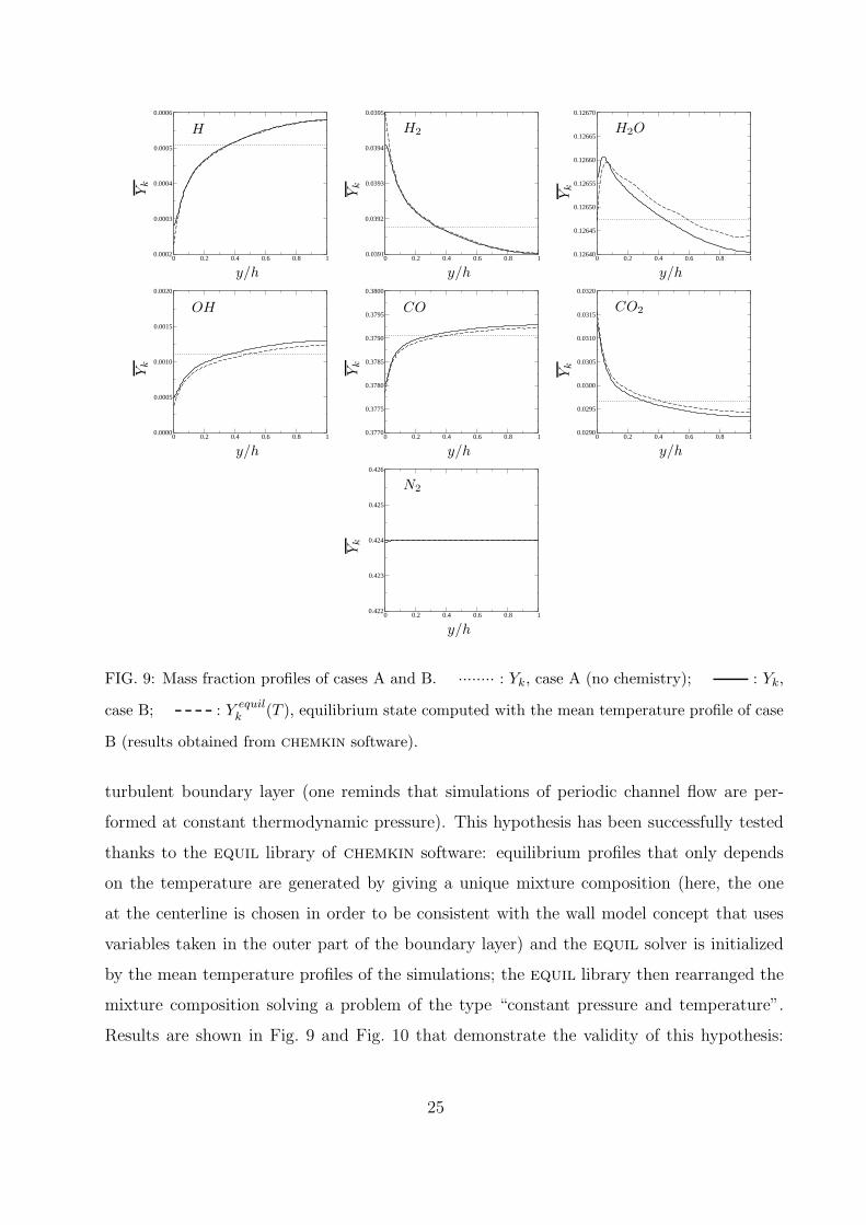
FIG. 9: Mass fraction profiles of cases A and B. ········ : Yk, case A (no chemistry); : Yk,
case B; : Y equilk (T ), equilibrium state computed with the mean temperature profile of case
B (results obtained from chemkin software).
turbulent boundary layer (one reminds that simulations of periodic channel flow are per-
formed at constant thermodynamic pressure). This hypothesis has been successfully tested
thanks to the equil library of chemkin software: equilibrium profiles that only depends
on the temperature are generated by giving a unique mixture composition (here, the one
at the centerline is chosen in order to be consistent with the wall model concept that uses
variables taken in the outer part of the boundary layer) and the equil solver is initialized
by the mean temperature profiles of the simulations; the equil library then rearranged the
mixture composition solving a problem of the type “constant pressure and temperature”.
Results are shown in Fig. 9 and Fig. 10 that demonstrate the validity of this hypothesis:
25
0 0.2 0.4 0.6 0.8 10.0000
0.0002
0.0004
0.0006
0.0008
0.0010
y/h
Yk
H
0 0.2 0.4 0.6 0.8 10.038
0.039
0.040
0.041
y/h
Yk
H2
0 0.2 0.4 0.6 0.8 10.08
0.10
0.12
0.14
y/h
Yk
H2O
0 0.2 0.4 0.6 0.8 10.0000
0.0005
0.0010
0.0015
0.0020
0.0025
0.0030
y/h
Yk
OH
0 0.2 0.4 0.6 0.8 10.36
0.37
0.38
0.39
y/h
Yk
CO
0 0.2 0.4 0.6 0.8 10.00
0.02
0.04
0.06
0.08
y/h
Yk
CO2
0 0.2 0.4 0.6 0.8 10.422
0.423
0.424
0.425
0.426
y/h
Yk
N2
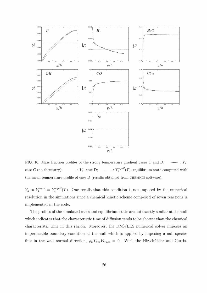
FIG. 10: Mass fraction profiles of the strong temperature gradient cases C and D. ········ : Yk,
case C (no chemistry); : Yk, case D; : Y equilk (T ), equilibrium state computed with
the mean temperature profile of case D (results obtained from chemkin software).
Yk ≈ Y equilk = Y equil
k (T ). One recalls that this condition is not imposed by the numerical
resolution in the simulations since a chemical kinetic scheme composed of seven reactions is
implemented in the code.
The profiles of the simulated cases and equilibrium state are not exactly similar at the wall
which indicates that the characteristic time of diffusion tends to be shorter than the chemical
characteristic time in this region. Moreover, the DNS/LES numerical solver imposes an
impermeable boundary condition at the wall which is applied by imposing a null species
flux in the wall normal direction, ρwYk,wVk,y,w = 0. With the Hirschfelder and Curtiss
26
0.01 0.1 1-2.5
-2
-1.5
-1
-0.5
0
0.5
y/h
Vk,y
h
m·s−
1i
H
0.01 0.1 10
0.005
0.01
0.015
0.02
y/h
Vk,y
h
m·s−
1i
H2
0.01 0.1 1-0.001
-0.0005
0
0.0005
0.001
0.0015
0.002
0.0025
y/h
Vk,y
h
m·s−
1i
H2O
0.01 0.1 1-1
-0.8
-0.6
-0.4
-0.2
0
0.2
y/h
Vk,y
h
m·s−
1i
OH
0.01 0.1 1-0.002
-0.0015
-0.001
-0.0005
0
0.0005
y/h
Vk,y
h
m·s−
1i
CO
0.01 0.1 1-0.01
0
0.01
0.02
0.03
0.04
0.05
y/h
Vk,y
h
m·s−
1i
CO2
0.01 0.1 1-0.001
-0.0005
0
0.0005
0.001
0.0015
0.002
y/h
Vk,y
h
m·s−
1i
N2
FIG. 11: Diffusion velocities of case B. : V hck,y; : Vk,y = V hc
k,y + V cory ; : V eglib
k,y .
(V hck,y and Vk,y perfectly collapse for species H and OH.)
approximation this implies:∂Xk
∂y
∣∣∣w
= 0 (19)
a result visible on the DNS and LES profiles. Discrepancies on chemkin profiles are ob-
served in the vicinity of the wall (y/h < 0.05) because this impermeable boundary condition
combined with the Hirschfelder and Curtiss approximation is not consistent with the chem-
ical equilibrium assumption postulated above when the temperature gradient is not null.
Indeed, making use of the equilibrium hypothesis, Eq. (19) can be rewritten as:
dXk
dT
∣∣∣eq
∂T
∂y
∣∣∣w
= 0 (20)
27
0.001 0.01 0.1 1-8
-6
-4
-2
0
2
y/h
Vk,y
h
m·s−
1i
H
0.001 0.01 0.1 1-0.005
0
0.005
0.01
0.015
0.02
0.025
y/h
Vk,y
h
m·s−
1i
H2
0.001 0.01 0.1 1-0.01
-0.008
-0.006
-0.004
-0.002
0
0.002
0.004
y/h
Vk,y
h
m·s−
1i
H2O
0.001 0.01 0.1 1-20
-10
0
10
20
y/h
Vk,y
h
m·s−
1i
OH
0.001 0.01 0.1 1-0.005
-0.004
-0.003
-0.002
-0.001
0
0.001
0.002
y/h
Vk,y
h
m·s−
1i
CO
0.001 0.01 0.1 1-0.02
0
0.02
0.04
0.06
0.08
y/h
Vk,y
h
m·s−
1i
CO2
0.001 0.01 0.1 1-0.001
-0.0005
0
0.0005
0.001
0.0015
0.002
y/h
Vk,y
h
m·s−
1i
N2
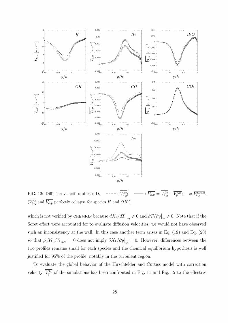
FIG. 12: Diffusion velocities of case D. : V hck,y; : Vk,y = V hc
k,y + V cory ; : V eglib
k,y .
(V hck,y and Vk,y perfectly collapse for species H and OH.)
which is not verified by chemkin because dXk/dT∣∣eq6= 0 and ∂T/∂y
∣∣w6= 0. Note that if the
Soret effect were accounted for to evaluate diffusion velocities, we would not have observed
such an inconsistency at the wall. In this case another term arises in Eq. (19) and Eq. (20)
so that ρwYk,wVk,y,w = 0 does not imply ∂Xk/∂y∣∣w
= 0. However, differences between the
two profiles remains small for each species and the chemical equilibrium hypothesis is well
justified for 95% of the profile, notably in the turbulent region.
To evaluate the global behavior of the Hirschfelder and Curtiss model with correction
velocity, V hcy of the simulations has been confronted in Fig. 11 and Fig. 12 to the effective
28
diffusion velocities of the simulations, Vk,y = V hck,y + V cor
y , and to the diffusion velocities
obtained by solving the full system Eq. (8) thanks to a post-processing with the eglib
library[68, 69] which solves the transport linear system with direct inversion. The latter are
noted V eglibk,y and represent the reference data. Except for species H2 and N2, we observe a
very good agreement between the effective diffusion velocities of the simulations and the ones
computed a priori with eglib. Moreover, comparing Vk,y and V hck,y we see that the correction
velocity modifies the Hirschfelder and Curtiss diffusion velocities, V hck,y, in the good direction.
This is clearly visible looking at profiles of species H2O, CO and CO2. Hence, the correction
velocity is not intrusive for the computation and the model retained in the numerical solver
to simulate mass diffusion is acceptable.
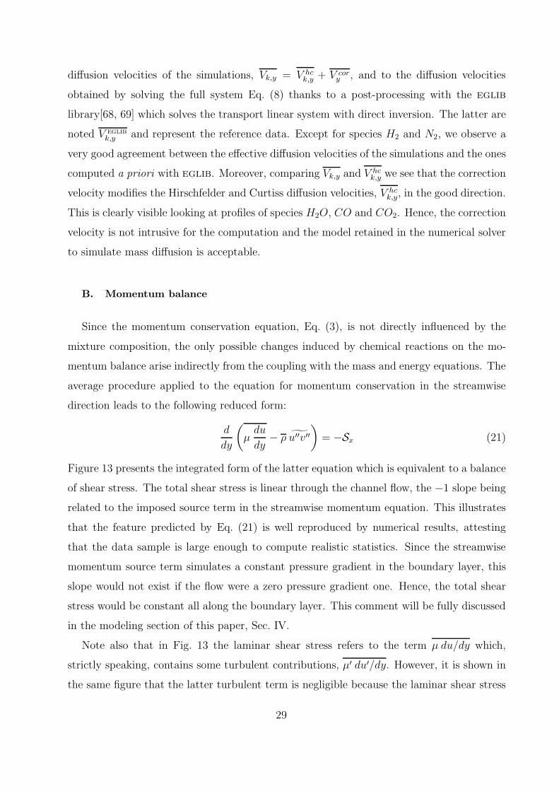
B. Momentum balance
Since the momentum conservation equation, Eq. (3), is not directly influenced by the
mixture composition, the only possible changes induced by chemical reactions on the mo-
mentum balance arise indirectly from the coupling with the mass and energy equations. The
average procedure applied to the equation for momentum conservation in the streamwise
direction leads to the following reduced form:
d
dy
(µ
du
dy− ρ u′′v′′
)= −Sx (21)
Figure 13 presents the integrated form of the latter equation which is equivalent to a balance
of shear stress. The total shear stress is linear through the channel flow, the −1 slope being
related to the imposed source term in the streamwise momentum equation. This illustrates
that the feature predicted by Eq. (21) is well reproduced by numerical results, attesting
that the data sample is large enough to compute realistic statistics. Since the streamwise
momentum source term simulates a constant pressure gradient in the boundary layer, this
slope would not exist if the flow were a zero pressure gradient one. Hence, the total shear
stress would be constant all along the boundary layer. This comment will be fully discussed
in the modeling section of this paper, Sec. IV.
Note also that in Fig. 13 the laminar shear stress refers to the term µ du/dy which,
strictly speaking, contains some turbulent contributions, µ′ du′/dy. However, it is shown in
the same figure that the latter turbulent term is negligible because the laminar shear stress
29
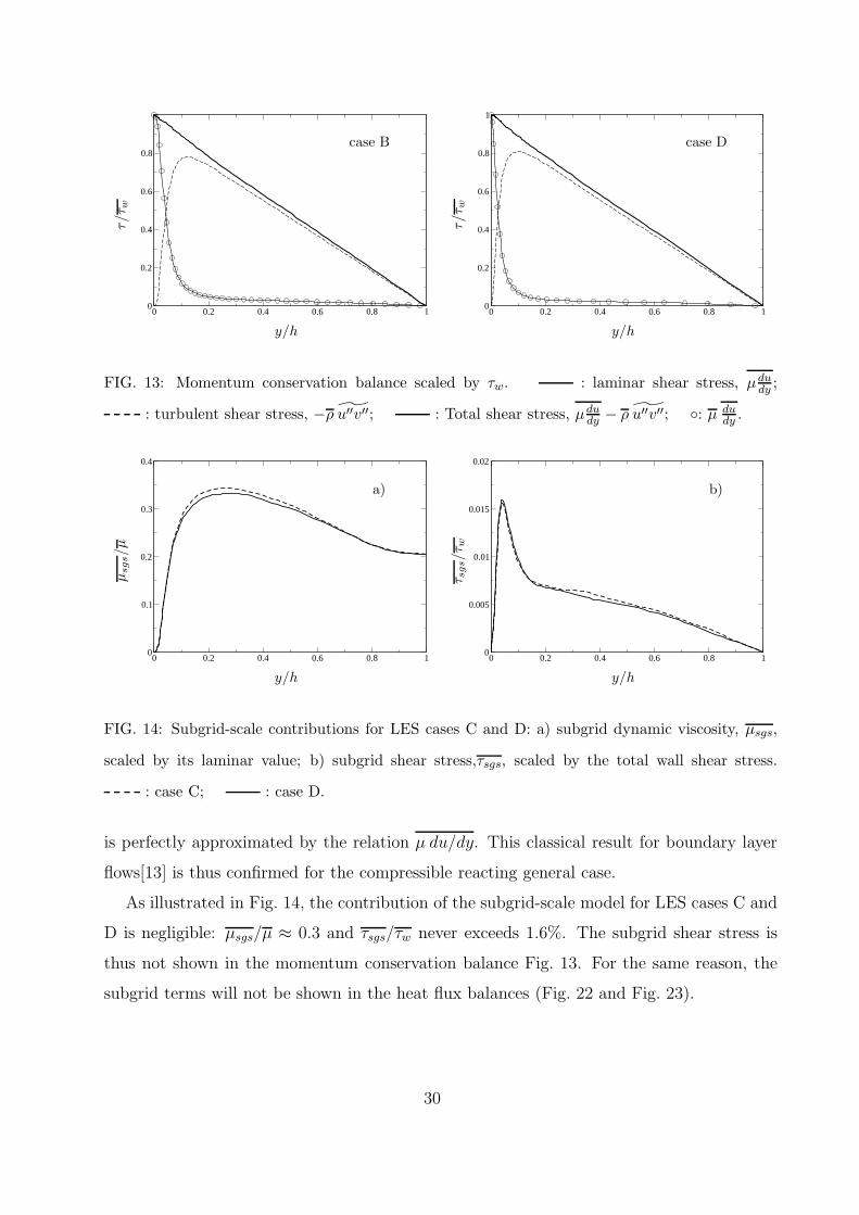
0 0.2 0.4 0.6 0.8 10
0.2
0.4
0.6
0.8
y/h
τ/τ w
case B
0 0.2 0.4 0.6 0.8 10
0.2
0.4
0.6
0.8
1
y/h
τ/τ w
case D
FIG. 13: Momentum conservation balance scaled by τw. : laminar shear stress, µdudy ;
: turbulent shear stress, −ρ u′′v′′; : Total shear stress, µdudy − ρ u′′v′′; : µ du
dy .
0 0.2 0.4 0.6 0.8 10
0.1
0.2
0.3
0.4
y/h
µsgs/µ
a)
0 0.2 0.4 0.6 0.8 10
0.005
0.01
0.015
0.02
y/h
τ sgs/τ w
b)
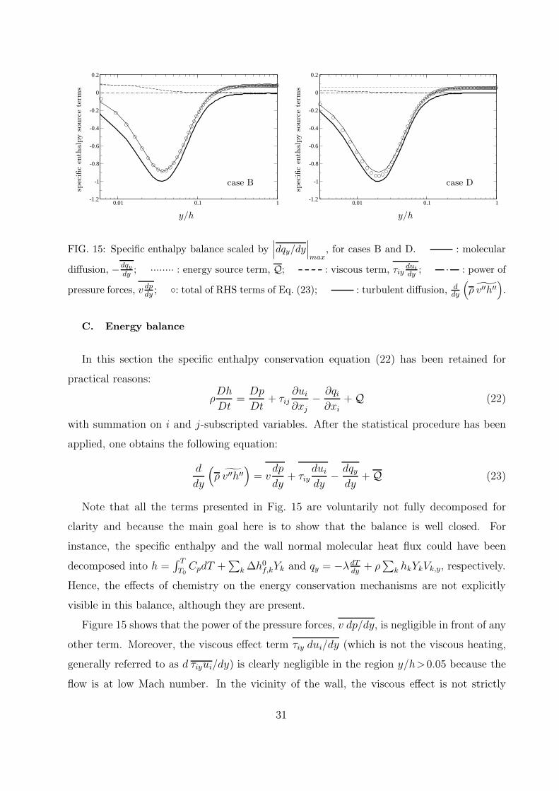
FIG. 14: Subgrid-scale contributions for LES cases C and D: a) subgrid dynamic viscosity, µsgs,
scaled by its laminar value; b) subgrid shear stress,τsgs, scaled by the total wall shear stress.
: case C; : case D.
is perfectly approximated by the relation µ du/dy. This classical result for boundary layer
flows[13] is thus confirmed for the compressible reacting general case.
As illustrated in Fig. 14, the contribution of the subgrid-scale model for LES cases C and
D is negligible: µsgs/µ ≈ 0.3 and τsgs/τw never exceeds 1.6%. The subgrid shear stress is
thus not shown in the momentum conservation balance Fig. 13. For the same reason, the
subgrid terms will not be shown in the heat flux balances (Fig. 22 and Fig. 23).
30
0.01 0.1 1-1.2
-1
-0.8
-0.6
-0.4
-0.2
0
0.2
y/h
spec
ific
enth
alp
yso
urc
ete
rms
case B
0.01 0.1 1-1.2
-1
-0.8
-0.6
-0.4
-0.2
0
0.2
y/h
spec
ific
enth
alp
yso
urc
ete
rms
case D
FIG. 15: Specific enthalpy balance scaled by∣∣∣dqy/dy
∣∣∣max
, for cases B and D. : molecular
diffusion, −dqy
dy ; ········ : energy source term, Q; : viscous term, τiyduidy ; : power of
pressure forces, v dpdy ; : total of RHS terms of Eq. (23); : turbulent diffusion, d
dy
(ρ v′′h′′
).
C. Energy balance
In this section the specific enthalpy conservation equation (22) has been retained for
practical reasons:
ρDh
Dt=
Dp
Dt+ τij
∂ui
∂xj
− ∂qi
∂xi
+ Q (22)
with summation on i and j-subscripted variables. After the statistical procedure has been
applied, one obtains the following equation:
d
dy
(ρ v′′h′′
)= v
dp
dy+ τiy
dui
dy− dqy
dy+ Q (23)
Note that all the terms presented in Fig. 15 are voluntarily not fully decomposed for
clarity and because the main goal here is to show that the balance is well closed. For
instance, the specific enthalpy and the wall normal molecular heat flux could have been
decomposed into h =∫ T
T0CpdT +
∑k ∆h0
f,kYk and qy = −λdTdy
+ ρ∑
k hkYkVk,y, respectively.
Hence, the effects of chemistry on the energy conservation mechanisms are not explicitly
visible in this balance, although they are present.
Figure 15 shows that the power of the pressure forces, v dp/dy, is negligible in front of any
other term. Moreover, the viscous effect term τiy dui/dy (which is not the viscous heating,
generally referred to as d τiyui/dy) is clearly negligible in the region y/h>0.05 because the
flow is at low Mach number. In the vicinity of the wall, the viscous effect is not strictly
31
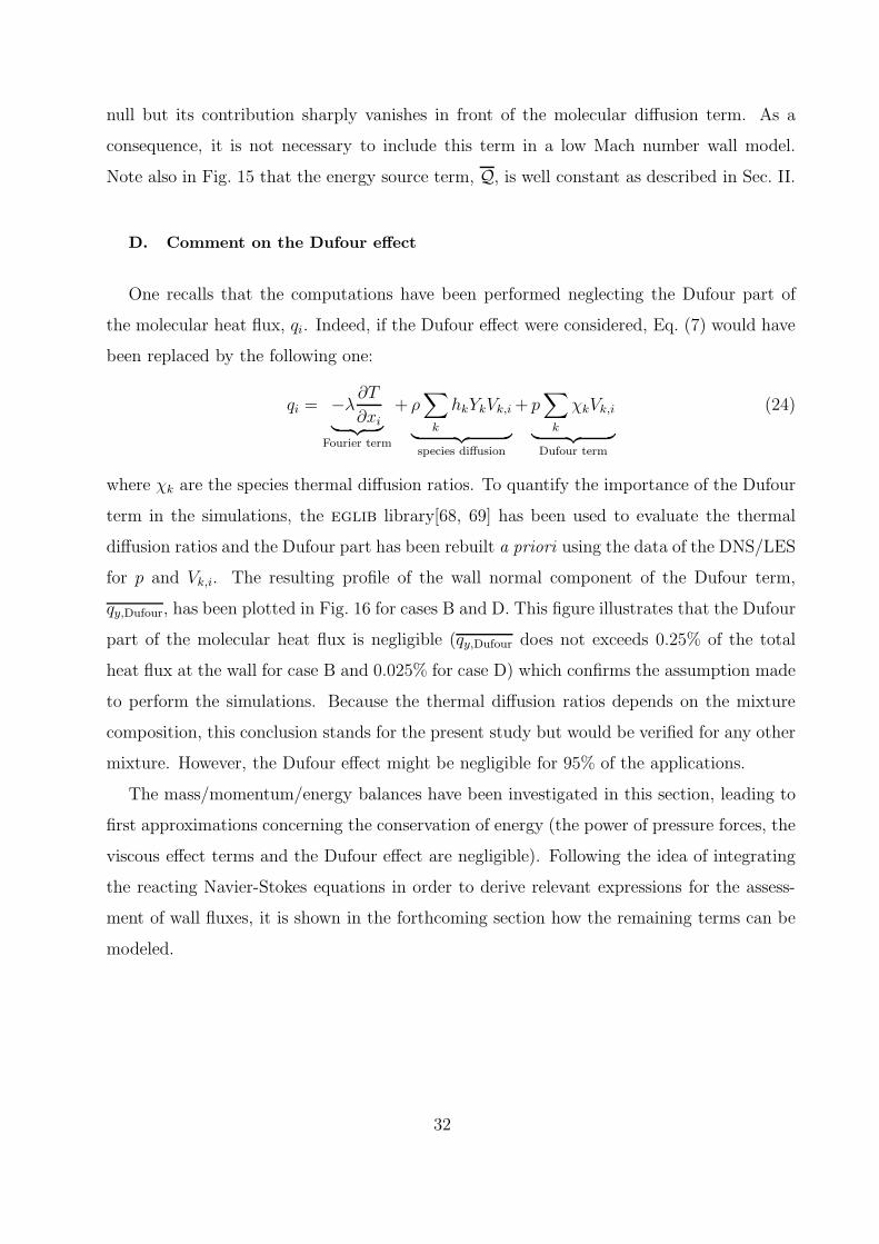
null but its contribution sharply vanishes in front of the molecular diffusion term. As a
consequence, it is not necessary to include this term in a low Mach number wall model.
Note also in Fig. 15 that the energy source term, Q, is well constant as described in Sec. II.
D. Comment on the Dufour effect
One recalls that the computations have been performed neglecting the Dufour part of
the molecular heat flux, qi. Indeed, if the Dufour effect were considered, Eq. (7) would have
been replaced by the following one:
qi = −λ∂T
∂xi︸ ︷︷ ︸Fourier term
+ ρ∑
k
hkYkVk,i
︸ ︷︷ ︸species diffusion
+ p∑
k
χkVk,i
︸ ︷︷ ︸Dufour term
(24)
where χk are the species thermal diffusion ratios. To quantify the importance of the Dufour
term in the simulations, the eglib library[68, 69] has been used to evaluate the thermal
diffusion ratios and the Dufour part has been rebuilt a priori using the data of the DNS/LES
for p and Vk,i. The resulting profile of the wall normal component of the Dufour term,
qy,Dufour, has been plotted in Fig. 16 for cases B and D. This figure illustrates that the Dufour
part of the molecular heat flux is negligible (qy,Dufour does not exceeds 0.25% of the total
heat flux at the wall for case B and 0.025% for case D) which confirms the assumption made
to perform the simulations. Because the thermal diffusion ratios depends on the mixture
composition, this conclusion stands for the present study but would be verified for any other
mixture. However, the Dufour effect might be negligible for 95% of the applications.
The mass/momentum/energy balances have been investigated in this section, leading to
first approximations concerning the conservation of energy (the power of pressure forces, the
viscous effect terms and the Dufour effect are negligible). Following the idea of integrating
the reacting Navier-Stokes equations in order to derive relevant expressions for the assess-
ment of wall fluxes, it is shown in the forthcoming section how the remaining terms can be
modeled.
32
0.01 0.1 10
0.0005
0.001
0.0015
0.002
0.0025
y/h
q y,D
ufo
ur/|q
w|
FIG. 16: Wall normal value of the Dufour heat flux computed a priori thanks to eglib library.
Results are scaled by the total heat flux at the wall. : case B; : case D.
IV. DEVELOPMENT OF WALL MODELS
Starting from the general flow equations, one seeks for two independent equations of the
type:df
dy= F ;
dg
dy= G (25)
where f and g stand for the total flux of momentum and energy in the y-direction respec-
tively. In their general formulation, the two functions f and g are dependent on the following
set of variables: (y, τw, qw, uout, Tout, Tw, Yk,out, Yk,w), where w-subscripted variables refer to
wall quantities and out-subscripted ones refer to outer flow conditions. If F and G are simple
functions of y, Eq. (25) can be integrated over space to generate a 2 × 2 non-linear system
of equations with qw and τw the unknowns. In other words, integrating Eq. (25) leads to
a law-of-the-wall which can be used to assess the momentum and energy fluxes at the wall
from the wall/outer flow conditions (uout, Tout, Tw, Yk,out and Yk,w). The simplest case would
be F = G = 0 but the case F = F0 and G = G0 where F0 and G0 are constant values also
leads to a suitable wall model. On the contrary, if F and/or G are/is unknown function of
y, Eq. (25) cannot be used to obtain a law-of-the-wall, as illustrated in Fig. 17.
The framework of this section follows five main assumptions for the flow: 1) the Reynolds
number is infinite so that no wake function will be considered to describe the outer part of
the boundary layer; 2) the Mach number is null; 3) no streamwise pressure gradients; 4) no
blowing or suction at the wall surface; 5) no roughness effect.
33
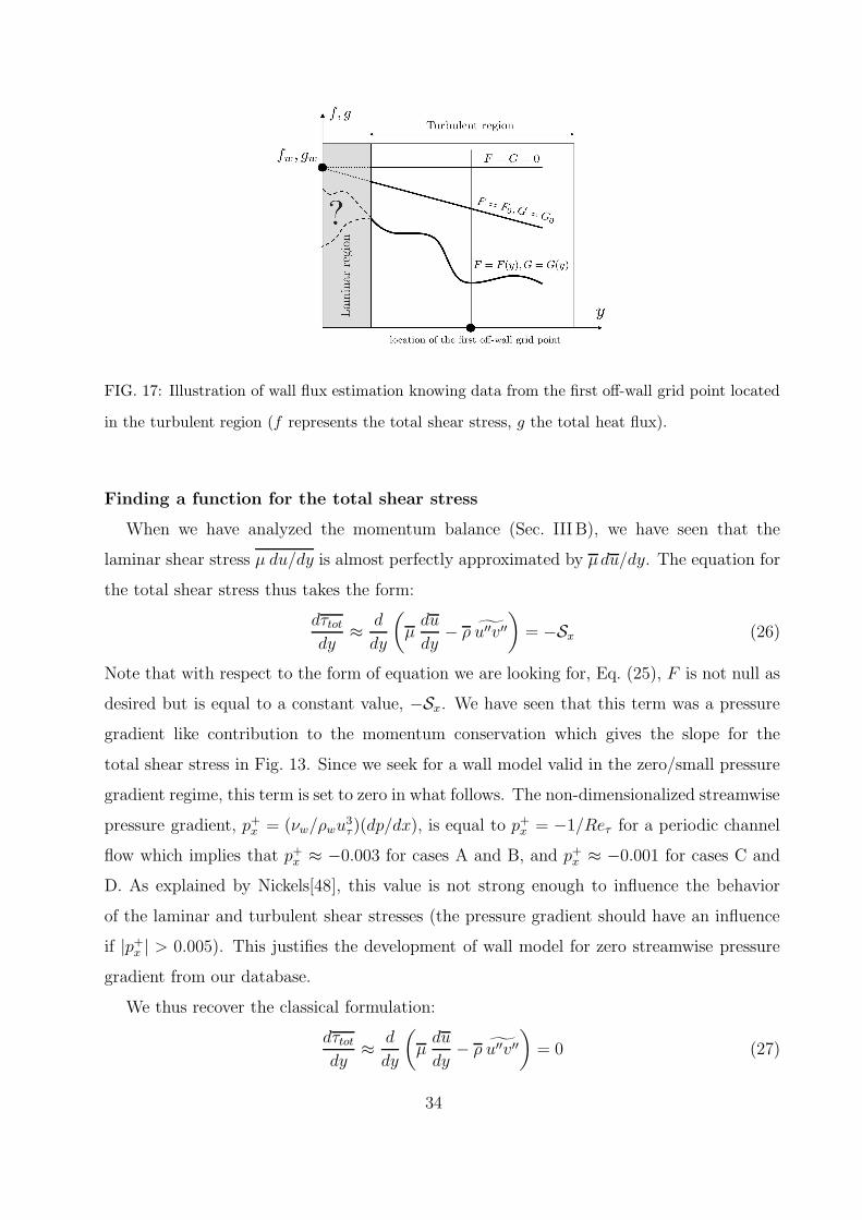
FIG. 17: Illustration of wall flux estimation knowing data from the first off-wall grid point located
in the turbulent region (f represents the total shear stress, g the total heat flux).
Finding a function for the total shear stress
When we have analyzed the momentum balance (Sec. III B), we have seen that the
laminar shear stress µ du/dy is almost perfectly approximated by µdu/dy. The equation for
the total shear stress thus takes the form:
dτtot
dy≈ d
dy
(µ
du
dy− ρ u′′v′′
)= −Sx (26)
Note that with respect to the form of equation we are looking for, Eq. (25), F is not null as
desired but is equal to a constant value, −Sx. We have seen that this term was a pressure
gradient like contribution to the momentum conservation which gives the slope for the
total shear stress in Fig. 13. Since we seek for a wall model valid in the zero/small pressure
gradient regime, this term is set to zero in what follows. The non-dimensionalized streamwise
pressure gradient, p+x = (νw/ρwu3
τ)(dp/dx), is equal to p+x = −1/Reτ for a periodic channel
flow which implies that p+x ≈ −0.003 for cases A and B, and p+
x ≈ −0.001 for cases C and
D. As explained by Nickels[48], this value is not strong enough to influence the behavior
of the laminar and turbulent shear stresses (the pressure gradient should have an influence
if |p+x | > 0.005). This justifies the development of wall model for zero streamwise pressure
gradient from our database.
We thus recover the classical formulation:
dτtot
dy≈ d
dy
(µ
du
dy− ρ u′′v′′
)= 0 (27)
34

0 0.2 0.4 0.6 0.8 10
0.05
0.1
0.15
0.2
y/h
l/h
l/h
=0.41
y/h
l/h = 0.12
FIG. 18: Mixing-length, computed as l =(−u′′v′′
)1/2/(du/dy), scaled by the channel half-height.
: case A; ········ : case B; : case C; : case D; A: Hoyas and Jimenez[35],
Reτ = 2000; p: Osterlund et al.[53], error bars representing a 95% confidence interval; E: An-
dersen et al.[76].
where the turbulent shear stress −ρ u′′v′′ can be approximated with the classical Boussi-
nesq assumption combined with a Prandtl mixing-length model for the turbulent dynamic
viscosity, µt. Hence, the turbulent shear stress can be modeled by:
−ρ u′′v′′ ≈ µtdu
dy≈ ρl2
(du
dy
)2
(28)
where l denotes the mixing-length. For near wall flows, it has been shown that the mixing-
length scales with the distance to the wall following the relation l = κy, with κ the von
Karman constant whose value is usually assumed to be 0.41. This value has been criticized
because some studies have shown that κ can change with the Reynolds number. This is
not consistent with the classical log-law, u+ = 1/κ ln y+ + C, which is not a function of
Re. However, the experiments of Osterlund et al.[53] have raised this confusion showing
that the classical log-law formulation is no longer Re-dependent if κ is set to 0.38 and
the additive constant, C, to 4.1 (this result has latter been confirmed by the study of
Buschmann and Gad-el-Hak[54]). Nevertheless, the values retained in this study for κ and
C will remain the most classical ones, κ = 0.41 and C = 5.5 for wall-bounded flows (C = 5.2
for external boundary layer), mainly because this has little influence on the final prediction
of u+. Indeed, a computation of the error (u+O − u+
c )/u+c , u+
O being the value advocated
by Osterlund et al. and u+c the classical one, leads to an expression that depends on y+:
35
(u+O − u+
c )/u+c = (0.19 ln y+ − 1.4)/(2.44 ln y+ + 5.5); the error does not exceed 5% for
50 < y+ < 108 (the two profiles are shown in Fig. 20 untill y+ = 103).
Figure 18 demonstrates the efficiency of the relation l = κy. Results from cases A, B,
C and D are confronted to the numerical result of Hoyas and Jimenez[35] as well as to
the experimental measurements of Andersen et al.[76] and Osterlund et al.[53]. As in the
classical theory[77], we first note that the mixing length scales reasonably well with the
channel half-height (or equivalently the boundary layer height for external flows) since all
the profiles collapse. Moreover, our results are consistent with the ones of the high friction
Reynolds number channel flow of Hoyas and Jimenez[35] and with the external boundary
layer of Osterlund et al.[53]. The profile of Andersen et al.[76] for zero pressure gradient
shows some discrepancies with others profiles but the trend remains unchanged: the von
Karman constant reproduces the mixing-length fairly well up to y/h ≈ 0.2, with or without
chemical reactions and significant heat transfer. For y/h > 0.2, the mixing-length is no
longer dependent on the distance from the wall and tends to a constant value (l/h ≈ 0.12
from our simulations) which is also a classical result[77]. The sudden increase of l in the
center region is due to du/dy that tends to zero at the centerline.
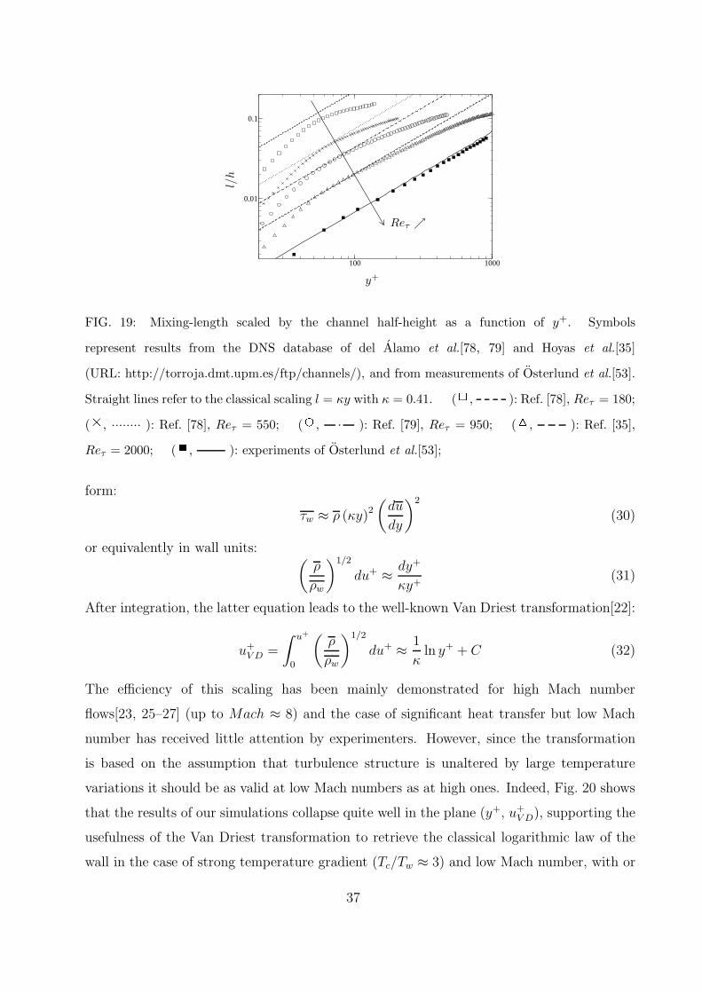
Figure 19 shows the mixing length as a function of y+ and illustrates that the collapse
with the von Karman model is enhanced when the Reynolds number increases. This supports
the use of the relation l = κy for developing wall models which are designed to handle large
Reynolds number flows. Moreover this figure demonstrates that when the friction Reynolds
number is too weak, Reτ = 180 for instance, the simulation is not representative of an
infinite Reynolds number boundary layer because the mixing length never matches with
the von Karman model. Hence, the higher the Reτ of the simulation is, the better is the
validation of the wall model with a priori tests.
Thus, the use of the von Karman constant is justified to develop wall models. Integrating
Eq. (27) over space, one obtains:
τw ≈ µdu
dy+ ρ (κy)2
(du
dy
)2
(29)
where the constant total shear stress τtot has been replaced by its wall value τw because
Eq. (27) indicates that the total shear stress is constant throughout the wall region, i.e.
τtot ≡ τw. Neglecting the laminar contribution, because in the context of wall modeling the
first off-wall point has to be in the fully turbulent region, we finally recover the classical
36
100 1000
0.01
0.1
y+
l/h
Reτ ր
FIG. 19: Mixing-length scaled by the channel half-height as a function of y+. Symbols
represent results from the DNS database of del Alamo et al.[78, 79] and Hoyas et al.[35]
(URL: http://torroja.dmt.upm.es/ftp/channels/), and from measurements of Osterlund et al.[53].
Straight lines refer to the classical scaling l = κy with κ = 0.41. (, ): Ref. [78], Reτ = 180;
(, ········ ): Ref. [78], Reτ = 550; (E, ): Ref. [79], Reτ = 950; (A, ): Ref. [35],
Reτ = 2000; (p, ): experiments of Osterlund et al.[53];
form:
τw ≈ ρ (κy)2
(du
dy
)2
(30)
or equivalently in wall units: (ρ
ρw
)1/2
du+ ≈ dy+
κy+(31)
After integration, the latter equation leads to the well-known Van Driest transformation[22]:
u+V D =
∫ u+
0
(ρ
ρw
)1/2
du+ ≈ 1
κln y+ + C (32)
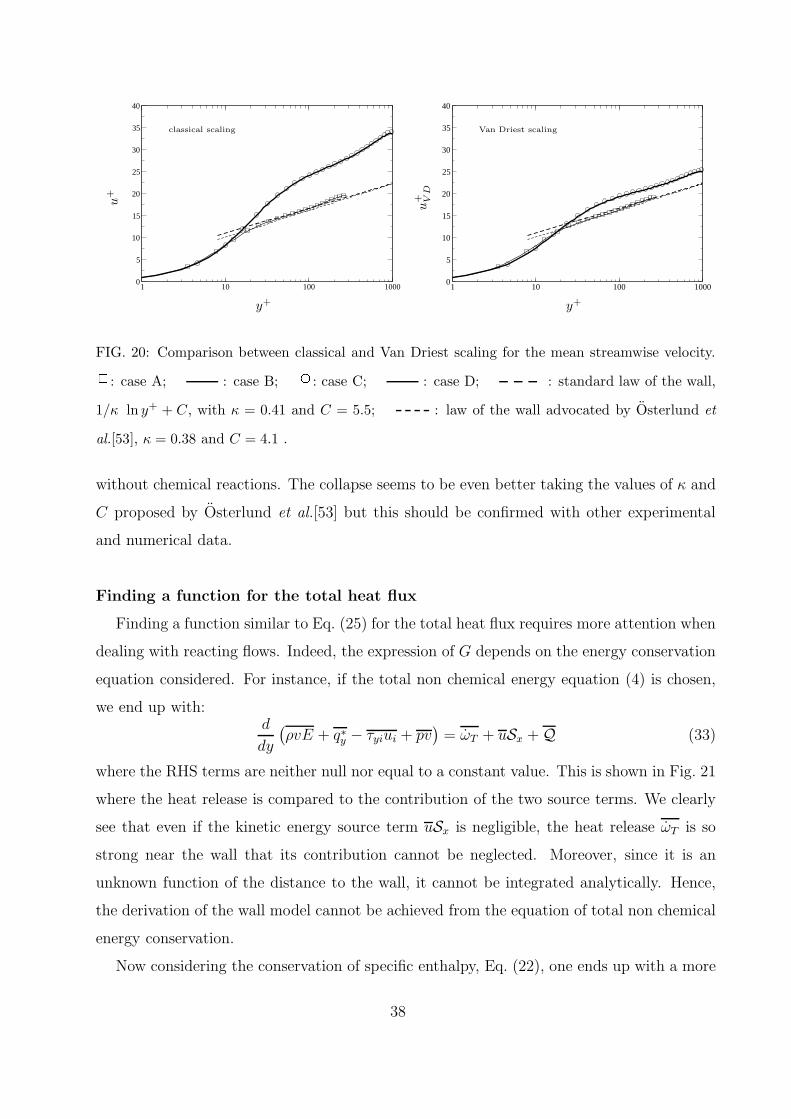
The efficiency of this scaling has been mainly demonstrated for high Mach number
flows[23, 25–27] (up to Mach ≈ 8) and the case of significant heat transfer but low Mach
number has received little attention by experimenters. However, since the transformation
is based on the assumption that turbulence structure is unaltered by large temperature
variations it should be as valid at low Mach numbers as at high ones. Indeed, Fig. 20 shows
that the results of our simulations collapse quite well in the plane (y+, u+V D), supporting the
usefulness of the Van Driest transformation to retrieve the classical logarithmic law of the
wall in the case of strong temperature gradient (Tc/Tw ≈ 3) and low Mach number, with or
37
1 10 100 10000
5
10
15
20
25
30
35
40
y+
u+
classical scaling
1 10 100 10000
5
10
15
20
25
30
35
40
y+
u+ V
D
Van Driest scaling
FIG. 20: Comparison between classical and Van Driest scaling for the mean streamwise velocity.: case A; : case B; E: case C; : case D; : standard law of the wall,
1/κ ln y+ + C, with κ = 0.41 and C = 5.5; : law of the wall advocated by Osterlund et
al.[53], κ = 0.38 and C = 4.1 .
without chemical reactions. The collapse seems to be even better taking the values of κ and
C proposed by Osterlund et al.[53] but this should be confirmed with other experimental
and numerical data.
Finding a function for the total heat flux
Finding a function similar to Eq. (25) for the total heat flux requires more attention when
dealing with reacting flows. Indeed, the expression of G depends on the energy conservation
equation considered. For instance, if the total non chemical energy equation (4) is chosen,
we end up with:d
dy
(ρvE + q∗y − τyiui + pv
)= ωT + uSx + Q (33)
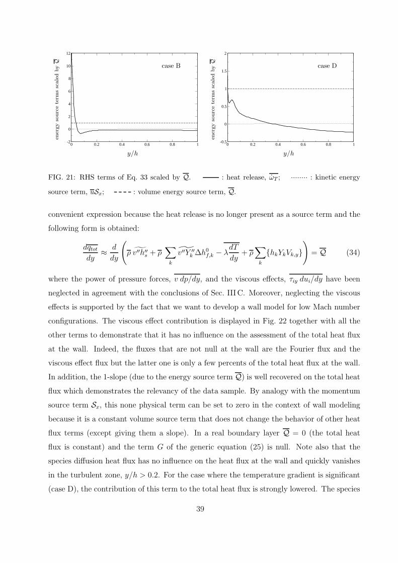
where the RHS terms are neither null nor equal to a constant value. This is shown in Fig. 21
where the heat release is compared to the contribution of the two source terms. We clearly
see that even if the kinetic energy source term uSx is negligible, the heat release ωT is so
strong near the wall that its contribution cannot be neglected. Moreover, since it is an
unknown function of the distance to the wall, it cannot be integrated analytically. Hence,
the derivation of the wall model cannot be achieved from the equation of total non chemical
energy conservation.
Now considering the conservation of specific enthalpy, Eq. (22), one ends up with a more
38
0 0.2 0.4 0.6 0.8 1-2
0
2
4
6
8
10
12
y/h
ener
gy
sourc
ete
rms
scale
dbyQ
case B
0 0.2 0.4 0.6 0.8 1-0.5
0
0.5
1
1.5
2
y/h
ener
gy
sourc
ete
rms
scale
dbyQ
case D
FIG. 21: RHS terms of Eq. 33 scaled by Q. : heat release, ωT ; ········ : kinetic energy
source term, uSx; : volume energy source term, Q.
convenient expression because the heat release is no longer present as a source term and the
following form is obtained:
dqtot
dy≈ d
dy
(ρ v′′h′′
s + ρ∑
k
v′′Y ′′k ∆h0
f,k − λdT
dy+ ρ
∑
k
hkYkVk,y)
= Q (34)
where the power of pressure forces, v dp/dy, and the viscous effects, τiy dui/dy have been
neglected in agreement with the conclusions of Sec. IIIC. Moreover, neglecting the viscous
effects is supported by the fact that we want to develop a wall model for low Mach number
configurations. The viscous effect contribution is displayed in Fig. 22 together with all the
other terms to demonstrate that it has no influence on the assessment of the total heat flux
at the wall. Indeed, the fluxes that are not null at the wall are the Fourier flux and the
viscous effect flux but the latter one is only a few percents of the total heat flux at the wall.
In addition, the 1-slope (due to the energy source term Q) is well recovered on the total heat
flux which demonstrates the relevancy of the data sample. By analogy with the momentum
source term Sx, this none physical term can be set to zero in the context of wall modeling
because it is a constant volume source term that does not change the behavior of other heat
flux terms (except giving them a slope). In a real boundary layer Q = 0 (the total heat
flux is constant) and the term G of the generic equation (25) is null. Note also that the
species diffusion heat flux has no influence on the heat flux at the wall and quickly vanishes
in the turbulent zone, y/h > 0.2. For the case where the temperature gradient is significant
(case D), the contribution of this term to the total heat flux is strongly lowered. The species
39
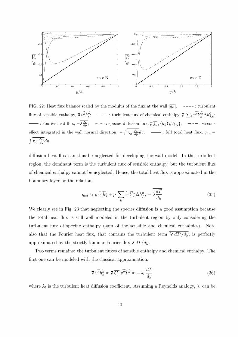
0 0.2 0.4 0.6 0.8 1-1
-0.8
-0.6
-0.4
-0.2
0
y/h
q/|q w
|
case B
0 0.2 0.4 0.6 0.8 1-1
-0.8
-0.6
-0.4
-0.2
0
y/h
q/|q w
|
case D
FIG. 22: Heat flux balance scaled by the modulus of the flux at the wall |qw|. : turbulent
flux of sensible enthalpy, ρ v′′h′′s ; : turbulent flux of chemical enthalpy, ρ
∑k v′′Y ′′
k ∆h0f,k;
: Fourier heat flux, −λdTdy ; ········ : species diffusion flux, ρ
∑khkYkVk,y; : viscous
effect integrated in the wall normal direction, −∫
τiyduidy dy; : full total heat flux, qtot −
∫τiy
duidy dy.
diffusion heat flux can thus be neglected for developing the wall model. In the turbulent
region, the dominant term is the turbulent flux of sensible enthalpy, but the turbulent flux
of chemical enthalpy cannot be neglected. Hence, the total heat flux is approximated in the
boundary layer by the relation:
qtot ≈ ρ v′′h′′s + ρ
∑
k
v′′Y ′′k ∆h0
f,k − λdT
dy(35)
We clearly see in Fig. 23 that neglecting the species diffusion is a good assumption because
the total heat flux is still well modeled in the turbulent region by only considering the
turbulent flux of specific enthalpy (sum of the sensible and chemical enthalpies). Note
also that the Fourier heat flux, that contains the turbulent term λ′ dT ′/dy, is perfectly
approximated by the strictly laminar Fourier flux λ dT/dy.
Two terms remains: the turbulent fluxes of sensible enthalpy and chemical enthalpy. The
first one can be modeled with the classical approximation:
ρ v′′h′′s ≈ ρ Cp v′′T ′′ ≈ −λt
dT
dy(36)
where λt is the turbulent heat diffusion coefficient. Assuming a Reynolds analogy, λt can be
40
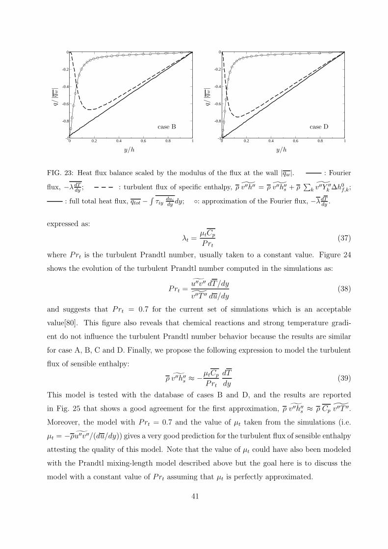
0 0.2 0.4 0.6 0.8 1-1
-0.8
-0.6
-0.4
-0.2
0
y/h
q/|q w
|
case B
0 0.2 0.4 0.6 0.8 1-1
-0.8
-0.6
-0.4
-0.2
0
y/h
q/|q w
|
case D
FIG. 23: Heat flux balance scaled by the modulus of the flux at the wall |qw|. : Fourier
flux, −λdTdy ; : turbulent flux of specific enthalpy, ρ v′′h′′ = ρ v′′h′′
s + ρ∑
k v′′Y ′′k ∆h0
f,k;
: full total heat flux, qtot −∫
τiyduidy dy; : approximation of the Fourier flux, −λdT
dy .
expressed as:
λt =µtCp
Prt
(37)
where Prt is the turbulent Prandtl number, usually taken to a constant value. Figure 24
shows the evolution of the turbulent Prandtl number computed in the simulations as:
Prt =u′′v′′ dT/dy
v′′T ′′ du/dy(38)
and suggests that Prt = 0.7 for the current set of simulations which is an acceptable
value[80]. This figure also reveals that chemical reactions and strong temperature gradi-
ent do not influence the turbulent Prandtl number behavior because the results are similar
for case A, B, C and D. Finally, we propose the following expression to model the turbulent
flux of sensible enthalpy:
ρ v′′h′′s ≈ −µtCp
Prt
dT
dy(39)
This model is tested with the database of cases B and D, and the results are reported
in Fig. 25 that shows a good agreement for the first approximation, ρ v′′h′′s ≈ ρ Cp v′′T ′′.
Moreover, the model with Prt = 0.7 and the value of µt taken from the simulations (i.e.
µt = −ρu′′v′′/(du/dy)) gives a very good prediction for the turbulent flux of sensible enthalpy
attesting the quality of this model. Note that the value of µt could have also been modeled
with the Prandtl mixing-length model described above but the goal here is to discuss the
model with a constant value of Prt assuming that µt is perfectly approximated.
41
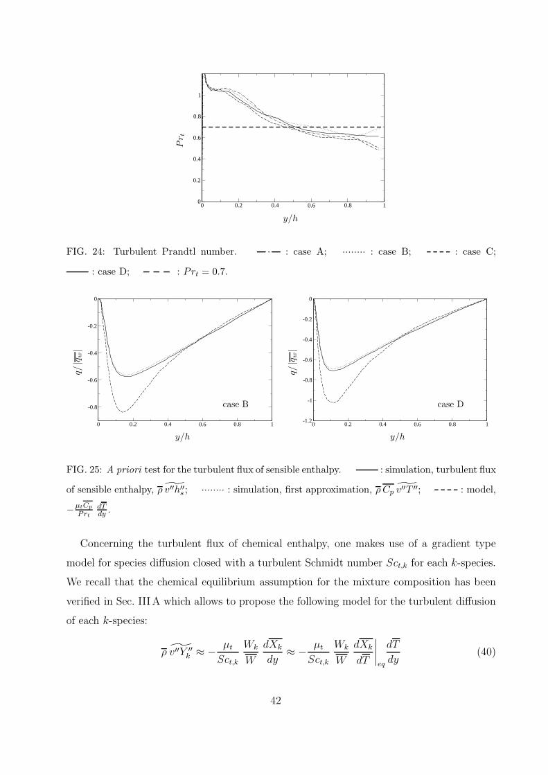
0 0.2 0.4 0.6 0.8 10
0.2
0.4
0.6
0.8
1
y/h
Pr t
FIG. 24: Turbulent Prandtl number. : case A; ········ : case B; : case C;
: case D; : Prt = 0.7.
0 0.2 0.4 0.6 0.8 1
-0.8
-0.6
-0.4
-0.2
0
y/h
q/|q w
|
case B
0 0.2 0.4 0.6 0.8 1-1.2
-1
-0.8
-0.6
-0.4
-0.2
0
y/h
q/|q w
|
case D
FIG. 25: A priori test for the turbulent flux of sensible enthalpy. : simulation, turbulent flux
of sensible enthalpy, ρ v′′h′′s ; ········ : simulation, first approximation, ρ Cp v′′T ′′; : model,
−µtCp
Prt
dTdy .
Concerning the turbulent flux of chemical enthalpy, one makes use of a gradient type
model for species diffusion closed with a turbulent Schmidt number Sct,k for each k-species.
We recall that the chemical equilibrium assumption for the mixture composition has been
verified in Sec. IIIA which allows to propose the following model for the turbulent diffusion
of each k-species:
ρ v′′Y ′′k ≈ − µt
Sct,k
Wk
W
dXk
dy≈ − µt
Sct,k
Wk
W
dXk
dT
∣∣∣∣eq
dT
dy(40)
42
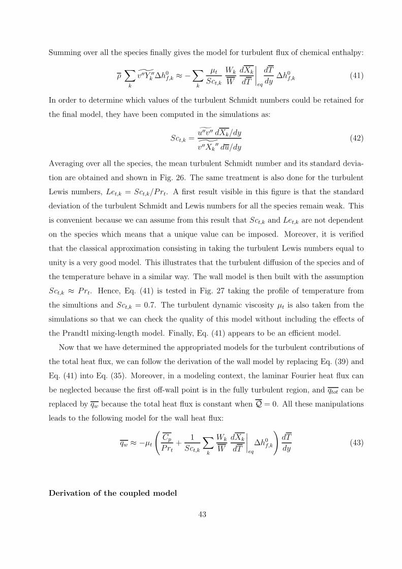
Summing over all the species finally gives the model for turbulent flux of chemical enthalpy:
ρ∑
k
v′′Y ′′k ∆h0
f,k ≈ −∑
k
µt
Sct,k
Wk
W
dXk
dT
∣∣∣∣eq
dT
dy∆h0
f,k (41)
In order to determine which values of the turbulent Schmidt numbers could be retained for
the final model, they have been computed in the simulations as:
Sct,k =u′′v′′ dXk/dy
v′′Xk′′ du/dy
(42)
Averaging over all the species, the mean turbulent Schmidt number and its standard devia-
tion are obtained and shown in Fig. 26. The same treatment is also done for the turbulent
Lewis numbers, Let,k = Sct,k/Prt. A first result visible in this figure is that the standard
deviation of the turbulent Schmidt and Lewis numbers for all the species remain weak. This
is convenient because we can assume from this result that Sct,k and Let,k are not dependent
on the species which means that a unique value can be imposed. Moreover, it is verified
that the classical approximation consisting in taking the turbulent Lewis numbers equal to
unity is a very good model. This illustrates that the turbulent diffusion of the species and of
the temperature behave in a similar way. The wall model is then built with the assumption
Sct,k ≈ Prt. Hence, Eq. (41) is tested in Fig. 27 taking the profile of temperature from
the simultions and Sct,k = 0.7. The turbulent dynamic viscosity µt is also taken from the
simulations so that we can check the quality of this model without including the effects of
the Prandtl mixing-length model. Finally, Eq. (41) appears to be an efficient model.
Now that we have determined the appropriated models for the turbulent contributions of
the total heat flux, we can follow the derivation of the wall model by replacing Eq. (39) and
Eq. (41) into Eq. (35). Moreover, in a modeling context, the laminar Fourier heat flux can
be neglected because the first off-wall point is in the fully turbulent region, and qtot can be
replaced by qw because the total heat flux is constant when Q = 0. All these manipulations
leads to the following model for the wall heat flux:
qw ≈ −µt
(Cp
Prt+
1
Sct,k
∑
k
Wk
W
dXk
dT
∣∣∣∣eq
∆h0f,k
)dT
dy(43)
Derivation of the coupled model
43
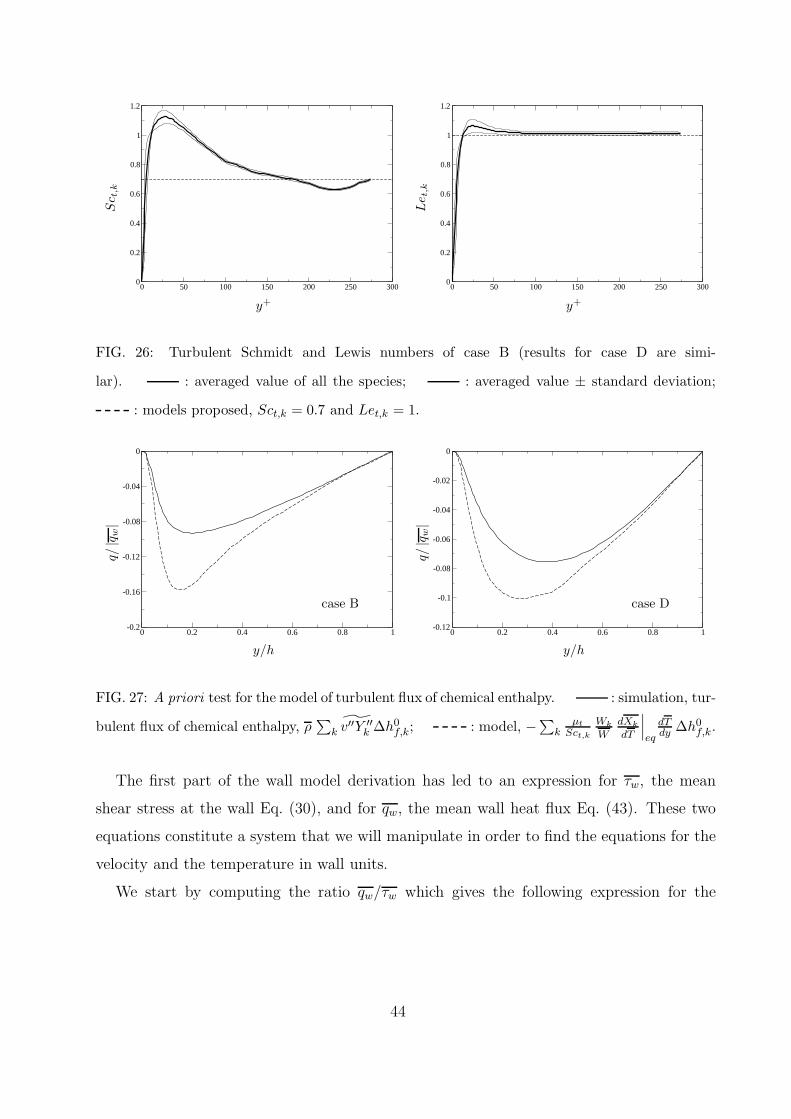
0 50 100 150 200 250 3000
0.2
0.4
0.6
0.8
1
1.2
y+
Sc t
,k
0 50 100 150 200 250 3000
0.2
0.4
0.6
0.8
1
1.2
y+
Le t
,k
FIG. 26: Turbulent Schmidt and Lewis numbers of case B (results for case D are simi-
lar). : averaged value of all the species; : averaged value ± standard deviation;
: models proposed, Sct,k = 0.7 and Let,k = 1.
0 0.2 0.4 0.6 0.8 1-0.2
-0.16
-0.12
-0.08
-0.04
0
y/h
q/|q w
|
case B
0 0.2 0.4 0.6 0.8 1-0.12
-0.1
-0.08
-0.06
-0.04
-0.02
0
y/h
q/|q w
|
case D
FIG. 27: A priori test for the model of turbulent flux of chemical enthalpy. : simulation, tur-
bulent flux of chemical enthalpy, ρ∑
k v′′Y ′′k ∆h0
f,k; : model, −∑kµt
Sct,k
Wk
WdXk
dT
∣∣∣eq
dTdy ∆h0
f,k.
The first part of the wall model derivation has led to an expression for τw, the mean
shear stress at the wall Eq. (30), and for qw, the mean wall heat flux Eq. (43). These two
equations constitute a system that we will manipulate in order to find the equations for the
velocity and the temperature in wall units.
We start by computing the ratio qw/τw which gives the following expression for the
44
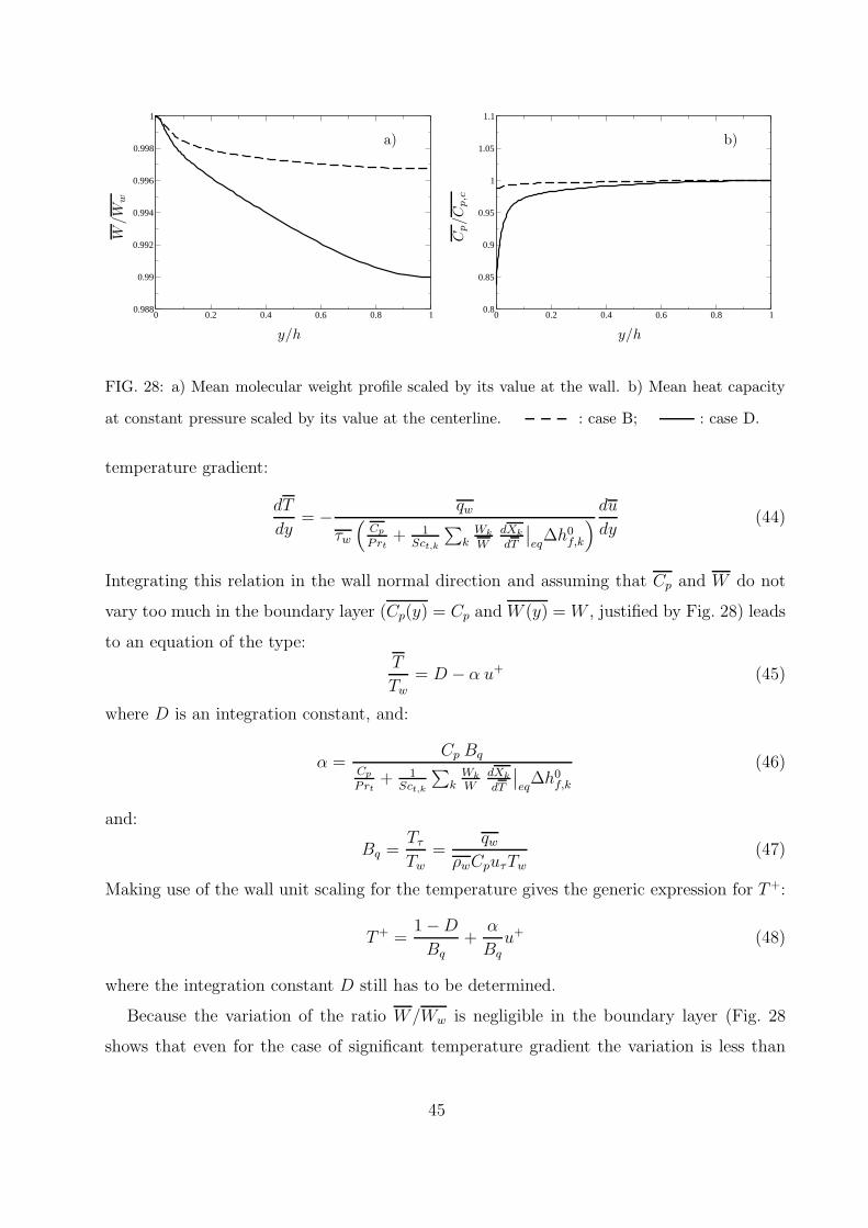
0 0.2 0.4 0.6 0.8 10.988
0.99
0.992
0.994
0.996
0.998
1
a)
y/h
W/W
w
0 0.2 0.4 0.6 0.8 10.8
0.85
0.9
0.95
1
1.05
1.1
b)
y/h
Cp/C
p,c
FIG. 28: a) Mean molecular weight profile scaled by its value at the wall. b) Mean heat capacity
at constant pressure scaled by its value at the centerline. : case B; : case D.
temperature gradient:
dT
dy= − qw
τw
(Cp
Prt+ 1
Sct,k
∑k
Wk
W
dXk
dT
∣∣eq
∆h0f,k
) du
dy(44)
Integrating this relation in the wall normal direction and assuming that Cp and W do not
vary too much in the boundary layer (Cp(y) = Cp and W (y) = W , justified by Fig. 28) leads
to an equation of the type:T
Tw= D − α u+ (45)
where D is an integration constant, and:
α =Cp Bq
Cp
Prt+ 1
Sct,k
∑k
Wk
WdXk
dT
∣∣eq
∆h0f,k
(46)
and:
Bq =Tτ
Tw
=qw
ρwCpuτTw
(47)
Making use of the wall unit scaling for the temperature gives the generic expression for T+:
T+ =1 − D
Bq+
α
Bqu+ (48)
where the integration constant D still has to be determined.
Because the variation of the ratio W/Ww is negligible in the boundary layer (Fig. 28
shows that even for the case of significant temperature gradient the variation is less than
45
1%), we can use the equation of state for perfect gas and write ρ/ρw ≈ Tw/T . Thanks to
this relation and Eq. (45), the Van Driest transformation Eq. (32) can be integrated as:
∫ u+
0
(Tw
T
)1/2
du+ =
∫ u+
0
(1
D − α u+
)1/2
du+ =1
κln y+ + C (49)
which finally gives an equation for u+:
2
α
(√D −
√D − α u+
)=
1
κln y+ + C (50)
We now have the two equations of the coupled wall model, Eq. (50) and Eq. (48), but
we still have to determine the two constants C and D in order to complete the development
of the wall model. Concerning the first one, we have seen in Fig. 20 that the classical value
C = 5.5 for wall-bounded flow can be assumed (the value C = 5.2 being reserved for external
boundary layers), associated with κ = 0.41. Note that the values advocated by Osterlund
et al.[53], κ = 0.38 and C = 4.1, could have been also retained.
The constant D is determined by imposing the wall model to recover the classical loga-
rithmic formulations for velocity and temperature for non-reacting isothermal flows. Hence,
D must satisfy two constraints:
• a) when Bq → 0 (i.e. the flow tends to be isothermal), one must have D → 1 to
recover the classical logarithmic law for velocity;
• b) when Bq → 0, Eq. (48) must be bounded. For instance, this can be verified if
(1 − D)/Bq is a constant that does not depend on Bq.
Because in a turbulent boundary layer the temperature profile is sensitive to the molecular
Prandtl number[77], one decides to pose:
1 − D
Bq= K(Pr) (51)
where K(Pr) is a constant that only depends on the molecular Prandtl number. In this
way, the two constraints for D are satisfied. Hence, when Bq → 0 (isothermal case) and
α → PrtBq (no chemistry) the two equations, Eq. (50) and Eq. (48), tends to the classical
logarithmic formulations (u+ = 1/κ ln y+ +C and T+ = Prt/κ ln y+ + constant(Pr)). To go
further in the determination of the K(Pr) constant, one chooses to make use of the Kader’s
function[8] as the reference equation for temperature profile because it takes into account
46
the effect of the molecular Prandtl number in its formulation (for 6×10⁻³ < Pr < 40×103).
When the laminar part of the Kader’s function tends to zero, the turbulent part remains
and we have:
T+K = 2.12 ln y+ + β(Pr) (52)
where β(Pr) is a function of the molecular Prandtl number defined as:
β(Pr) =(3.85 Pr1/3 − 1.3
)2+ 2.12 lnPr (53)
One arbitrarily decides to determine the K(Pr) constant by minimizing the square difference
between Eq.(52) and Eq.(48) (i.e.(T+ − T+
K
)2) in the limit Bq → 0 and α → PrtBq, for
100 < y+ < 200. This leads to an analytical expression for K(Pr):
K(Pr) = β(Pr) − PrtC +
(Prt
κ− 2.12
)(1 − 2 ln(20)) (54)
Hence, the wall model is able to take into account the effects of the molecular Prandtl
number, the strong temperature gradients, and the chemical reactions while being consistent
with the classical logarithmic formulations for velocity and temperature.
Now that all the terms of the wall model are defined one can proceed to the evaluation
of its efficiency performing a priori tests.
A priori tests
Knowing a set of outer conditions (uout, Tout, Yk,out) at the wall distance yout, and the
temperature at the wall Tw it is possible to invert the system of equations, Eq. (48) and
Eq. (50), to assess the wall fluxes. In order to test the efficiency of this coupled wall
model several sets of outer conditions have been built from the mean profiles of the present
simulations (the mean velocity, mean temperature and mean mass fraction profiles are used
to generate uout, Tout, and Yk,out, respectively). The wall fluxes resulting from the inversion
of the coupled wall model can then be confronted to their exact values taken from the
simulations. The parameters used for the inversion are summed up in table IX where R
is the perfect gas constant, Ww
∣∣eq
=∑
k Xk,w
∣∣eq
Wk is the molecular weight of the mixture
at the wall determined with the equilibrium assumption, Cp,w
∣∣eq
=∑
k Cp,kYk,w
∣∣eq
is the
heat capacity at constant pressure evaluated at the wall from the wall temperature (which
is a known value) and the equilibrium concentration profiles, and Wout =∑
k Xk,outWk the
molecular weight at the outer condition. Note that because the pressure is constant in the
47
0 0.2 0.4 0.6 0.8 10.4
0.6
0.8
1
1.2
1.4
yout/h
model
vs.
sim
ulatio
ncase A
0 0.2 0.4 0.6 0.8 10.4
0.6
0.8
1
1.2
1.4
yout/h
model
vs.
sim
ulatio
n
case B
0 0.2 0.4 0.6 0.8 10.5
1
1.5
2
2.5
yout/h
model
vs.
sim
ulatio
n
case C
0 0.2 0.4 0.6 0.8 10.5
1
1.5
2
2.5
yout/h
model
vs.
sim
ulatio
n
case D
FIG. 29: Wall heat flux and viscous stress scaled by their exact counterparts from the DNS/LES.
: τw from the new wall model; : qw from the new wall model; : τw from the
standard law-of-the-wall, u+ = 1/κ ln y+ + C; : qw from the Kader correlation[8], Eq. (52).
boundary layer, the outer pressure pout is used to determine the wall density. Results are
shown in Fig. 29. In these plots, the predicted wall shear stress, τmodelw , and wall heat flux,
qmodelw , are scaled by their exact DNS/LES counterparts. The values given by the standard
wall function for mean velocity and by the Kader’s correlation for temperature[8] are also
plotted to illustrate the efficiency of the new model. Note that in Fig. 29 the determination
of qw from the Kader function, Eq. (52), is done by determining y+ thanks to the classical
law-of-the-wall for velocity.
For all the cases, the coupled wall model is more efficient than standard functions: the
48
TABLE IX: Set of variables retained for the inversion of the law-of-the-wall Eq. (48) and Eq. (50).
κ C K(Pr) Prt Sct,k ρw Cp W
0.41 5.5 −0.5 0.7 0.7 Tw Ww
∣∣eq
/R pout Cp,w
∣∣eq
Wout
new model exhibits a large plateau for yout > 0.2h where the error is a few percents (between
5% and 20%, say). Of course profiles vanish for yout < 0.2h because the wall model is not
expected to hold in the viscous sublayer. In case A, the effects of variable density and
chemistry are not present which explains a good collapse of both the new and standard
models. In the case of multicomponent reacting flow with smooth temperature gradient
(case B), the model clearly improves the prediction which shows that the chemical part of
the model behaves well: with the new wall model, the error on the wall heat flux prediction
is damped to 5% whereas the error is around 20% for the standard model.
Concerning the strong temperature gradient cases C and D, the standard functions com-
mit an error of 100% and 60% on the wall shear stress and heat flux respectively. These
predictions are clearly improved by the new wall model developed herein which works pretty
well without chemistry and strong temperature variations (in case C, errors are lowered to
15% for the wall shear stress and 10% for the wall heat flux) and shows a moderate discrep-
ancy when chemical reactions are considered (case D).
The current model has been developed under the assumption of a flow at infinite Reynolds
number. The DNS/LES are at moderate Reynolds number which could explain the little
discrepancies observed in these a priori tests. Moreover, one recall that no specific tuning
of the free coefficients has been done because the aim of this study is to obtain a law-of-the-
wall with appropriate dependancies and scaling between the wall unknowns and the outer
variables. For instance, the error in the prediction of the wall heat flux can be lowered by
8% for case D, taking Prt = 0.65 (which would fit better the DNS data than Prt = 0.7),
and the values advocated by Osterlund et al.[53] for C and κ.
Hence, the velocity/temperature/chemistry coupled law-of-the-wall developed in this
study appears to behave well with reacting flows at low Mach number, with or without
temperature gradient which opens a wide range of numerical investigations (by RANS
calculations) for industrial applications in such a flow configuration.
49
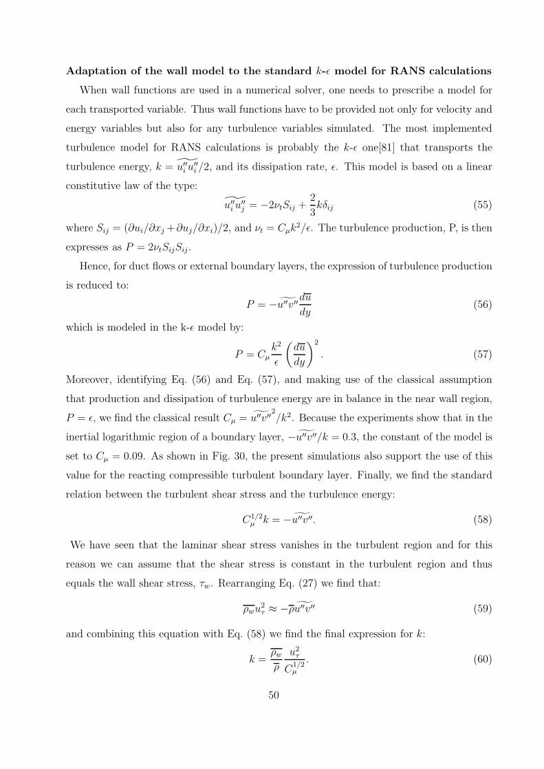
Adaptation of the wall model to the standard k-ǫ model for RANS calculations
When wall functions are used in a numerical solver, one needs to prescribe a model for
each transported variable. Thus wall functions have to be provided not only for velocity and
energy variables but also for any turbulence variables simulated. The most implemented
turbulence model for RANS calculations is probably the k-ǫ one[81] that transports the
turbulence energy, k = u′′i u
′′i /2, and its dissipation rate, ǫ. This model is based on a linear
constitutive law of the type:
u′′i u
′′j = −2νtSij +
2
3kδij (55)
where Sij = (∂ui/∂xj +∂uj/∂xi)/2, and νt = Cµk2/ǫ. The turbulence production, P, is then
expresses as P = 2νtSijSij .
Hence, for duct flows or external boundary layers, the expression of turbulence production
is reduced to:
P = −u′′v′′du
dy(56)
which is modeled in the k-ǫ model by:
P = Cµk2
ǫ
(du
dy
)2
. (57)
Moreover, identifying Eq. (56) and Eq. (57), and making use of the classical assumption
that production and dissipation of turbulence energy are in balance in the near wall region,
P = ǫ, we find the classical result Cµ = u′′v′′2/k2. Because the experiments show that in the
inertial logarithmic region of a boundary layer, −u′′v′′/k = 0.3, the constant of the model is
set to Cµ = 0.09. As shown in Fig. 30, the present simulations also support the use of this
value for the reacting compressible turbulent boundary layer. Finally, we find the standard
relation between the turbulent shear stress and the turbulence energy:
C1/2µ k = −u′′v′′. (58)
We have seen that the laminar shear stress vanishes in the turbulent region and for this
reason we can assume that the shear stress is constant in the turbulent region and thus
equals the wall shear stress, τw. Rearranging Eq. (27) we find that:
ρwu2τ ≈ −ρu′′v′′ (59)
and combining this equation with Eq. (58) we find the final expression for k:
k =ρw
ρ
u2τ
C1/2µ
. (60)
50
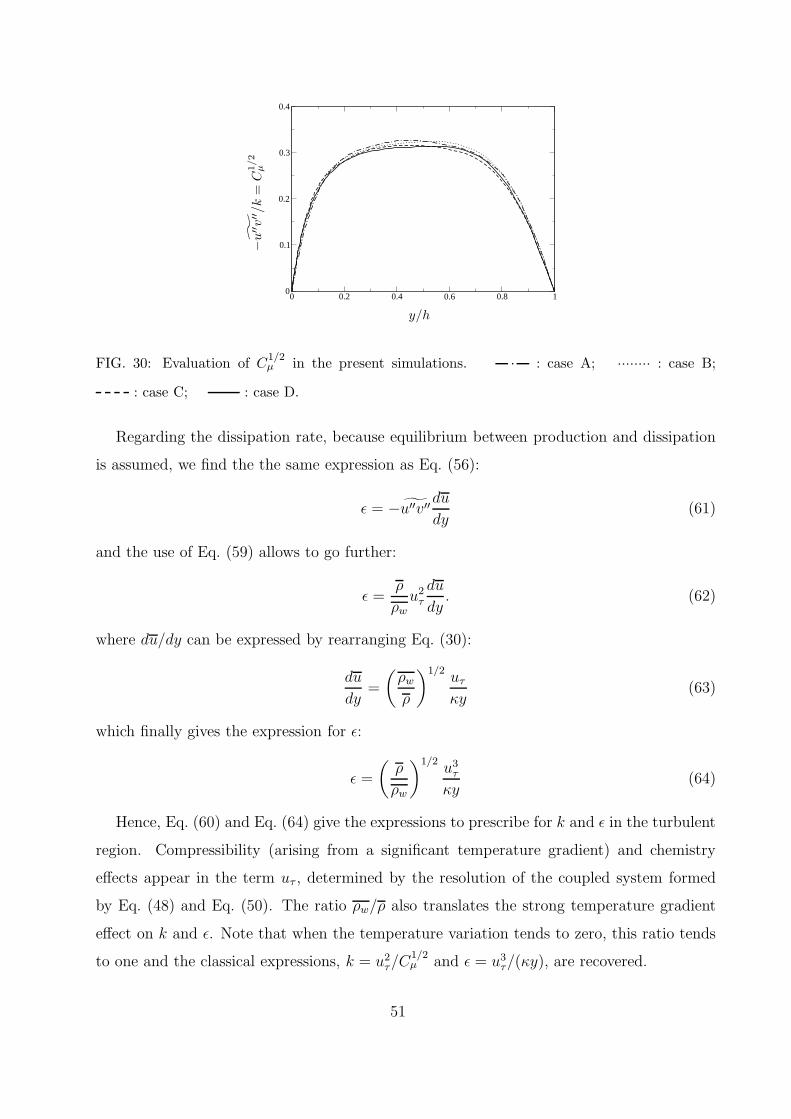
0 0.2 0.4 0.6 0.8 10
0.1
0.2
0.3
0.4
y/h
−u′′v′′/k
=C
1/2
µ
FIG. 30: Evaluation of C1/2µ in the present simulations. : case A; ········ : case B;
: case C; : case D.
Regarding the dissipation rate, because equilibrium between production and dissipation
is assumed, we find the the same expression as Eq. (56):
ǫ = −u′′v′′du
dy(61)
and the use of Eq. (59) allows to go further:
ǫ =ρ
ρw
u2τ
du
dy. (62)
where du/dy can be expressed by rearranging Eq. (30):
du
dy=
(ρw
ρ
)1/2uτ
κy(63)
which finally gives the expression for ǫ:
ǫ =
(ρ
ρw
)1/2u3
τ
κy(64)
Hence, Eq. (60) and Eq. (64) give the expressions to prescribe for k and ǫ in the turbulent
region. Compressibility (arising from a significant temperature gradient) and chemistry
effects appear in the term uτ , determined by the resolution of the coupled system formed
by Eq. (48) and Eq. (50). The ratio ρw/ρ also translates the strong temperature gradient
effect on k and ǫ. Note that when the temperature variation tends to zero, this ratio tends
to one and the classical expressions, k = u2τ/C
1/2µ and ǫ = u3
τ/(κy), are recovered.
51

The integration of these two expressions into a numerical solver depends of course of
the numerical method retained but we remind that Eq. (60) and Eq. (64) are only valid in
the logarithmic region. For a cell-centered solver, it could be interesting to combine these
equations with the method proposed by Craft et al.[50, 52] to account for a correct behavior
of k and ǫ till the wall, and so in the laminar region.
V. CONCLUSIONS
The current paper presents a set of DNS and wall-resolved LES of periodic plane channel
flow that constitutes a reference database for analyzing mean behavior of wall turbulence in
the case of multicomponent reacting flows at low Mach number, with or without compress-
ibility effect (the compressibility being due to a strong temperature gradient).
The study has revealed that the classical assumptions for boundary layer flows are still
valid for multicomponent reacting flows, among them: the efficiency of the Boussinesq as-
sumption combined with the Prandtl mixing-length for modeling the turbulent shear stress;
the validity of the Van Driest transformation up to a temperature ratio of 3; and the efficiency
of the Reynolds analogy for modeling the turbulent flux of sensible enthalpy. Moreover, it
has been demonstrated that the power of pressure forces and the viscous effect terms could
be neglected in the process of energy conservation.
This work has also presented some new findings concerning the multicomponent part of
the Navier-Stokes equations for turbulent boundary layer flows. First, it appears that the
composition of the mixture is at the equilibrium state which strongly simplifies the modeling.
Second, the molecular species diffusion is negligible in the turbulent region. Third, a model
for the turbulent flux of chemical enthalpy has been proposed and successfully validated. In
addition, the turbulent Prandtl number appears to be insensitive to the chemical reactions
and the strong temperature gradient. The present data also confirm that taking the turbu-
lent Lewis number to unity is a good approximation which implies to take Sck,t = Prt. Note
finally that it has also been shown that the Dufour part of the molecular heat flux could be
neglected for such cases of study.
Simplifying the Navier-Stokes equations and replacing the turbulent terms by their
model conterpart, a new law-of-the-wall useable in RANS computations is proposed to
estimate the wall shear stress as well as the wall heat flux from the knowledge of a set
52
of outer/wall conditions. This formulation stands for the general case of multicomponent
reacting compressible turbulent flows and degrades in the classical formulations when the
temperature gradient tends to zero and the chemistry effects are null. This law-of-the-wall
also recognizes that the energy and momentum equations are coupled for large temperature
variations (i.e. large density variations) and gives reasonable results when confronted to
the DNS/LES database with a priori tests. Moreover, although the current work only
deals with one type of mixture (the species and the Prandtl number of the mixture are
unchanged), the law-of-the-wall has been developed without any assumption concerning the
species involved and the molecular Prandtl number. Thus this wall model should behave
well with any other mixture.
ACKNOWLEDGMENTS
The authors are grateful to CNRS/DGA for funding this work and want to acknowledge
the financial support and expertise of Snecma Propulsion Solide (SAFRAN group). We
want to thank the CINES (Centre Informatique National pour l’Enseignement Superieur)
for the access to supercomputer facilities. J.M. Deoclezian is also gratefully acknowledged
for fruitful discussions.
53
[1] L. Prandtl. Uber Flussigkeitsbewegung bei sehr kleiner Reibung. In Teubner, editor, Verhand-
lungen des dritten internationalen Mathematiker-Kongresses, pages 484–491, Leipzig, Ger-
many, 1905.
[2] H. Blasius. Boundary layers in fluids with small friction. Z. Math. Phys., 56:1–37, 1908.
[3] T. von Karman. Uber laminare und turbulente Reibung. Z. Angew. Math. Mech., pages
233–252, 1921.
[4] T. von Karman. Mechanische Ahnlichkeit und Turbulenz. Nach. Ges. Wiss. Gottingen, Math.
Phys. Klasse, pages 58–68, 1930.
[5] F. H. Clauser. The turbulent boundary layer. Advances Appl. Mech., 4:1–51, 1956.
[6] S. V. Patankar and D. B. Spalding. Heat and mass transfer in boundary layers. Morgan-
Grampian, London, 1967.
[7] C. A. Sleicher and M. W. Rouse. Convenient correlation for heat transfert to constant and
variable property fluids in turbulent pipe flow. Int. J. Heat Mass Transfer, 18(5):677–683,
May 1975.
[8] B. A. Kader. Temperature and concentration profiles in fully turbulent boundary layers. Int.
J. Heat Mass Transfer, 24(9):1541–1544, 1981.
[9] H. Fernholz and P. Finley. A critical compilation of compressible turbulent boundary layer
data. AGARD-AG, 223, 1977.
[10] P. Bradshaw. Compressible turbulent shear layers. Annu. Rev. Fluid Mech., 9:33–54, 1977.
[11] E. F. Spina, A. J. Smits, and S. K. Robinson. The physics of supersonic turbulent boundary
layers. Annu. Rev. Fluid Mech., 26:287–319, 1994.
[12] G. N. Coleman, Kim J., and R. D. Moser. A numerical study of turbulent supersonic
isothermal-wall channel flow. J. Fluid Mech., 305:159–183, 1995.
[13] P. G. Huang, G. N. Coleman, and P. Bradshaw. Compressible turbulent channel flows: DNS
results and modelling. J. Fluid Mech., 305:185–218, 1995.
[14] P. Moin and K. Mahesh. Direct numerical simulation: a tool in turbulence research. Annu.
Rev. Fluid Mech., 30:539–578, 1998.
[15] Y. Morinishi, S. Tamano, and K. Nakabayashi. Direct numerical simulation of compressible
turbulent channel flow between adiabatic and isothermal walls. J. Fluid Mech., 502:273–308,
54
2004.
[16] P. Moin and J. Kim. Numerical investigation of turbulent channel flow. J. Fluid Mech.,
118:341–377, 1982.
[17] S. Volker, R. D. Moser, and P. Venugopal. Optimal large eddy simulation of turbulent channel
flow based on direct numerical simulation statistical data. Phys. Fluids, 14(10):3675–3691,
October 2002.
[18] W. Wang and R. H. Pletcher. On the large eddy simulation of a turbulent channel flow with
significant heat transfer. Phys. Fluids, 8(12):3354–3366, December 1996.
[19] L. D. Dailey, N. Meng, and R. H. Pletcher. Large eddy simulation of constant heat flux
turbulent channel flow with property variations: quasi-developed model and mean flow results.
J. Heat Trans., 125(1):27–38, February 2003.
[20] C. Brun, M. P. Boiarciuc, M. Haberkorn, and P. Comte. Larde eddy simulation of compressible
channel flow. Theor. Comput. Fluid Dyn., 22(3-4):189–212, 2008.
[21] M. V. Morkovin. Effects of compressibility on turbulent flows. In A. Favre, editor, Mechanique
de la Turbulence, pages 367–380. 1961.
[22] E. R. Van Driest. Turbulent boundary layer in compressible fluids. J. Aero. Sci, 18(3):145–160,
216, March 1951.
[23] E. R. Keener and E. J. Hopkins. Van Driest generalization applied to turbulent skin friction
and velocity profiles measured on the wall of a Mach 7.4 wind tunnel. AIAA J., 11(12):1784–
1785, December 1973.
[24] H. Fernholz and P. Finley. A critical commentary on mean flow data for two-dimensional
compressible turbulent boundary layers. AGARD-AG, 253, 1980.
[25] P. G. Huang, P. Bradshaw, and T. J. Coakley. Skin friction and velocity profile family for
compressible turbulent boundary layers. AIAA J., 31(9):1600–1604, September 1993.
[26] R. M. C. So, H. S. Zhang, T. B. Gatski, and C. G. Speziale. Logarithmic laws for compressible
turbulent boundary layers. AIAA J., 32(11):2162–2168, November 1994.
[27] P. G. Huang and G. N. Coleman. Van driest transformation and compressible wall-bounded
flows. AIAA J., 32(10):2110–2113, 1994.
[28] F. Nicoud. Numerical study of a channel flow with variable properties. In Annual Research
Briefs, pages 289–310. Center for Turbulence Research, NASA Ames/Stanford Univ., 1998.
[29] M. P. Martın and G. V. Candler. DNS of a mach 4 boundary layer with chemical reactions.
55
AIAA Paper 2000-0399, Jan. 2000.
[30] M. P. Martın and G. V. Candler. Temperature-fluctuation scaling in reacting boundary
layers. In Annual Research Briefs, pages 151–162. Center for Turbulence Research, NASA
Ames/Stanford Univ., 2001.
[31] J. Kim, P. Moin, and R. Moser. Turbulence statistics in fully developed channel flow at low
Reynolds number. J. Fluid Mech., 177:133–166, 1987.
[32] R. K. Cheng and T. T. Ng. Some aspects of strongly heated turbulent boundary layer flow.
Phys. Fluids, 25(8):1333–1341, August 1982.
[33] R.D. Moser, J Kim, and N.N. Mansour. Direct numerical simulation of turbulent channel flow
up to Reτ = 590. Phys. Fluids, 11(4):943–945, 1999.
[34] M. Teitel and R. A. Antonia. Heat transfer in fully developed turbulent channel flow: com-
parison between experiment and direct numerical simulations. Int. J. Heat Mass Transfer,
36(6):1701–1706, 1993.
[35] S. Hoyas and J. Jimenez. Scaling the velocity fluctuations in turbulent channel up to Reτ =
2003. Phys. Fluids, 18(011702):18–21, 2006.
[36] J. Jimenez and R. D. Moser. What are we learning from simulating wall turbulence? Phil.
Trans. R. Soc. A, 365:715–732, 2007.
[37] B. Mohammadi and G. Puigt. Wall functions in computational fluid mechanics. Comput.
Fluids, 35(10):1108–1115, 2006.
[38] R. L. Simpson. Characteristics of turbulent boundary layers at low Reynolds numbers with
and without transpiration. J. Fluid Mech., 42(4):769–802, 1970.
[39] F. Nicoud and P. Bradshaw. A velocity transformation for heat and mass transfer. Phys.
Fluids, 12(1):237–238, Jan. 2000.
[40] C. S. Subramanian and R. A. Antonia. Effect of Reynolds number on a slightly heated
turbulent boundary layer. Int. J. Heat Mass Transfer, 24(11):1833–1846, 1981.
[41] Z. Han and R. D. Reitz. A temperature wall function formulation for variable-density turbulent
flows with application to engine convective heat transfer modeling. Int. J. Heat Mass Transfer,
40(3):613–625, 1997.
[42] T. H. Shih, L. A. Povinelli, N. S. Liu, M. G. Potapczuk, and J. L. Lumley. A generalized wall
function. NASA TM-1999-209398, July 1999.
[43] K. Suga, T. J. Craft, and H. Iacovides. An analytical wall-function for turbulent flows and
56
heat transfer over rough walls. Int. J. Heat Fluid Flow, 27(5):852–866, 2006.
[44] P. G. Huang and P. Bradshaw. Law of the wall for turbulent flows in pressure gradients.
AIAA J., 33(4):624–632, April 1995.
[45] M. Skote and D.S. Henningson. Analysis of the data base from a DNS of a separating turbulent
boundary layer. In Annual Research Briefs, pages 225–237. Center for Turbulence Research,
NASA Ames/Stanford Univ., 1999.
[46] M. Skote and D.S. Henningson. Direct numerical simulation of a separated turbulent boundary
layer. J. Fluid Mech., 471:107–136, 2002.
[47] T. H. Shih, L. A. Povinelli, and N. S. Liu. Application of generalized wall function for complex
turbulent flows. Journal of Turbulence, 4(15):1–16, April 2003.
[48] T.B. Nickels. Inner scaling for wall-bounded flows subject to large pressure gradients. J. Fluid
Mech., 521:217–239, 2004.
[49] T. Houra and Y. Nagano. Effects of adverse pressure gradient on heat transfer mechanism in
thermal boundary layer. Int. J. Heat Fluid Flow, 27:967–976, 2006.
[50] T. J. Craft, A. V. Gerasimov, H. Iacovides, and B. E. Launder. Progress in the generalization
of wall-function treatments. Int. J. Heat Fluid Flow, 23(2):148–160, 2002.
[51] T. J. Craft, S. E. Gant, H. Iacovides, and B. E. Launder. A new wall function strategy for
complex turbulent flows. Numer. Heat Transfer, 45(4):301–318, 2004.
[52] T. J. Craft, S. E. Gant, A. V. Gerasimov, H. Iacovides, and B. E. Launder. Development and
application of wall-function treatments for turbulent forced and mixed convection flows. Fluid
Dynamics Research, 38(2-3):127–144, 2006.
[53] J.M. Osterlund, A. V. Johansson, H. M. Nagib, and M. H. Hites. A note on the overlap region
in turbulent boundary layers. Phys. Fluids, 12(1):1–4, January 2000.
[54] M. H. Buschmann and M. Gad-el Hak. Debate concerning the mean-velocity profile of a
turbulent boundary layer. AIAA J., 41(4):565–572, April 2003.
[55] M. H. Buschmann and M. Gad-el Hak. Structure of the canonical turbulent wall-bounded
flow. AIAA J., 44(11):2500–2503, November 2006.
[56] P. A. Davidson, T. B. Nickels, and P. A. Krogstad. The logarithmic structure function law in
wall-layer turbulence. J. Fluid Mech., 550:51–60, 2006.
[57] M. H. Buschmann and M. Gad-el Hak. Generalized logarithmic law and its consequences.
AIAA J., 41(1):40–48, January 2003.
57
[58] S. V. Utyuzhnikov. Some new approaches to building and implementation of wall-functions
for modeling of near-wall turbulent flows. Comput. Fluids, 34:771–784, 2005.
[59] K. K. Kuo. Principles of combustion. John Wiley & Sons, Inc., Hoboken, New Jersey, 2nd
edition, 2005.
[60] T. Poinsot and D. Veynante. Theoretical and Numerical Combustion. Edwards, 2nd edition,
2005.
[61] J. Amaya, O. Cabrit, D. Poitou, B. Cuenot, and M. El Hafi. Unsteady coupling of Navier-
Stokes and radiative heat transfer solvers applied to an anisothermal multicomponent tur-
bulent channel flow. In Proceedings of Eurotherm 83 - Computational Thermal Radiation in
Participating Media III, Lisbon, Portugal, 15-17 April 2009.
[62] E. M. Sparrow, R. Eichhorn, and J. L. Gregg. Combined forced and free convection in a
boundary layer flow. Phys. Fluids, 2(3):319–328, 1959.
[63] F. Nicoud, J. C. Traineau, and M. Prevost. Evolution of heat flux with mass flow rate in
a subscale setup for the Ariane 5 solide rocket booster. In 2nd International Symposium
on Engineering Turbulence Modelling and Measurements, Florence (Italy), May 31 - June 2,
1993.
[64] B. E. Poling, J. M. Prausnitz, and J. P. O’Connell. The properties of gases and liquids.
McGraw-Hill, 5th edition, 2001.
[65] D. Y. Peng and D. B. Robinson. A new two-constant equation of state. Ind. Eng. Chem.,
Fundam., 15(1):59–64, 1976.
[66] J.O. Hirschfelder, F. Curtiss, and R.B. Bird. Molecular theory of gases and liquids. John
Wiley & Sons, 1964.
[67] V. Giovangigli. Multicomponent Flow Modeling. Birkhauser, 1999.
[68] A. Ern and V. Giovangigli. Multicomponent transport algorithms. Lecture Notes in Physics,
New Series Monographs, m 24. Springer-Verlag, Heidelberg, 1994.
[69] A. Ern and V. Giovangigli. Fast and accurate multicomponent transport property evaluation.
J. Comput. Phys., 120(1):105–116, August 1995.
[70] J. Jimenez and P. Moin. The minimal flow unit in near-wall turbulence. J. Fluid Mech.,
225:213–240, 1991.
[71] V. Moureau, G. Lartigue, Y. Sommerer, C. Angelberger, O. Colin, and T. Poinsot. Numerical
methods for unsteady compressible multi-component reacting flows on fixed and moving grids.
58
J. Comput. Phys., 202(2):710–736, 2005.
[72] P. Schmitt, T. Poinsot, B. Schuermans, and K. P. Geigle. Large-eddy simulation and exper-
imental study of heat transfer, nitric oxide emissions and combustion instability in a swirled
turbulent high-pressure burner. J. Fluid Mech., 570:17–46, 2007.
[73] S. Mendez and F. Nicoud. Large-eddy simulation of a bi-periodic turbulent flow with effusion.
J. Fluid Mech., 598:27–65, 2008.
[74] O. Colin and M. Rudgyard. Development of high-order Taylor-Galerkin schemes for unsteady
calculations. J. Comput. Phys., 162(2):338–371, 2000.
[75] F. Nicoud and F. Ducros. Subgrid-scale stress modelling based on the square of the velocity
gradient tensor. Flow, Turb. and Combustion, 62:183–200, 1999.
[76] P. S. Andersen, W. M. Kays, and R. J. Moffat. Experimental results for the transpired
turbulent boundary layer in an adverse pressure gradient. J. Fluid Mech., 69(2):353–375,
1975.
[77] W.M. Kays, M.E. Crawford, and B. Weigand. Convective Heat and Mass Transfer. McGraw-
Hill, 2004.
[78] J. C. del Alamo and J. Jimenez. Spectra of the very large anisotropic scales in turbulent
channels. Phys. Fluids, 15(6):L41–L44, 2003.
[79] J. C. del Alamo, J. Jimenez, P. Zandonade, and R. D. Moser. Scaling of the energy spectra
of turbulent channels. J. Fluid Mech., 500:135–144, 2004.
[80] K.C. Kays. Turbulent Prandtl number. Where are we ? J. Heat Trans., 116:284–295, May
1994.
[81] B. E. Launder and D. B. Spalding. The numerical computation of turbulent flows. Comput.
Methods Appl. Mech. Engng., 3(2):269–289, 1974.
59