Direct Simulation Based Model-Predictive Control ofFlow Maldistribution in Parallel Microchannels

Mathieu Martin Chris Patton John SchmittSourabh V. Apte∗

School of Mechanical, Industrial and Manufacturing EngineeringOregon State University

Corvallis, OR 97331

July 5, 2009

Abstract

Flow maldistribution, resulting from bubbles or other particulate matter, can leadto drastic performance degradation in devices that employ parallel microchannels forheat transfer. In this work, direct numerical simulations of fluid flow through a pre-scribed parallel microchannel geometry are performed and coupled with active controlof actuated microvalves to effectively identify and reduce flow maldistribution. Accu-rate simulation of fluid flow through a set of three parallel microchannels is achievedutilizing a fictitious domain representation of immersed objects, such as microvalvesand artificially introduced bubbles. Flow simulations are validated against experimentalresults obtained for flow through a single, high aspect ratio microchannel, flow aroundan oscillating cylinder, and flow with a bubble rising in an inclined channel. Resultsof these simulations compare very well to those obtained experimentally, and validatethe use of the solver for the parallel microchannel configuration of this study. Systemidentification techniques are employed on numerical simulations of fluid flow throughthe geometry to produce a lower dimensional model that captures the essential dynamicsof the full nonlinear flow, in terms of a relationship between valve angles and the exitflow rate for each channel. A model predictive controller is developed which employsthis reduced order model to identify flow maldistribution from exit flow velocities andprescribe actuation of channel valves to effectively redistribute the flow. Flow simula-tions with active control are subsequently conducted with artificially introduced bubbles.The model predictive control methodology is shown to adequately reduce flow maldistri-bution by quickly varying channel valves to remove bubbles and equalize flow rates ineach channel.

∗Corresponding Author: e-mail: sva@engr.orst.edu, phone: 541-737-7335, fax: 541-737-2600

1

1 Introduction

Microchannels are employed in a variety of devices, such as heat sinks and heat exchangers,to improve heat transfer effectiveness. For improved efficiency and cooling of high heat loads,two-phase flows involving convective boiling of high latent heat fluids are often used. Forma-tion of vapor bubbles inside the microchannel geometry can lead to blocking effects, resultingin flow maldistribution with non-uniform spatial and temporal conditions. Such flow mald-istribution reduces the effectiveness of the heat transfer, leading to decreased performanceof the devices under consideration.

Previous investigations into multiphase flow in microchannels [1, 2] have shown that thevapor phase can take different forms, each yielding qualitatively different flow behavior. Fortwo-phase flow in a square channel, Cubaud et al. [3] classify flow regimes by the size andoccupation of the channel by the vapor phase. In bubbly flow, small bubbles comprise avapor phase that is relatively small in comparison to the channel dimensions. In this flowregime, bubbles are mainly spherical and flow with the fluid at a similar velocity. Sharp& Adrian [4] investigated clogging or arching structures inside microchannels or in sharpcorners due to interaction of rigid particles. Bubble-laden flows may also lead to similarblocking effects in microchannel geometries.

In microchannel geometries using a liquid as a coolant for removal of high heat fluxes,bubbles may form and grow at nucleation sites. These bubbles remain attached to channelwalls due to surface tension effects [5]. Existence of the bubble in a channel affects thefluid flow not only in that channel, but also in all of the connected channels, leading toflow maldistribution. As the bubble grows, eventually the surface tension forces keeping thebubble attached to the wall are lowered; and the hydrodynamic forces acting on the bubblemay overcome any resistive forces, detaching and moving the bubble [6, 7]. Formation andgrowth of bubbles inside parallel microchannel geometries can lead to flow instabilities, flowreversals and can affect the flow distribution in a network of channels [8]. To mitigate theseflow instabilities, Mukherjee et al. [8] proposed use of a variable size microchannels withincreased cross-sectional areas in the downstream direction. Increasing areas in the down-stream directions result in higher pressures locally, which tend to reduce the flow reversal,and is an example of a passive control to mitigate flow distribution problems. Active control,based on model-predictive control algorithm, has been used by Bleris et al. [9], in order toimprove mixing of chemical species in parallel microchannels. By regulating the mass-flowrates in each channel, they showed how active control can be used to improve mixing andchemical reaction processes.

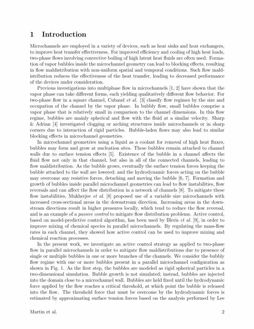
In the present work, we investigate an active control strategy as applied to two-phaseflow in parallel microchannels in order to mitigate flow maldistributions due to presence ofsingle or multiple bubbles in one or more branches of the channels. We consider the bubblyflow regime with one or more bubbles present in a parallel microchannel configuration asshown in Fig. 1. As the first step, the bubbles are modeled as rigid spherical particles in atwo-dimensional simulation. Bubble growth is not simulated; instead, bubbles are injectedinto the domain close to a microchannel wall. Bubbles are held fixed until the hydrodynamicforce applied by the flow reaches a critical threshold, at which point the bubble is releasedinto the flow. The threshold force that must be overcome by the hydrodynamic forces isestimated by approximating surface tension forces based on the analysis performed by Lee

Martin et al. 2

et al. [6]. Flow maldistribution resulting from bubble injection is regulated through actuationof valves at the entrance of each microchannel.

Figure 1: Schematic of parallel microchannels with bubbly flow.

The paper is structured as follows. Section 2 provides the mathematical foundation ofthe direct numerical simulations employed in this study. Details regarding implementation ofthe numerical algorithm employed are presented in Section 3. Control design methodology,including the means by which reduced order models are produced from direct numericalsimulations and the use of such models in a model predictive control scheme, is detailedin Section 4. Section 6 presents results of validation cases for the flow solver. Controlledflow simulations of bubbly flow are examined in Section 7, with conclusions and avenues forfuture work presented in Section 8.

2 Mathematical formulation

The computations carried out in this work utilize direct numerical simulation (DNS) withfictitious domain representation of arbitrary shaped immersed objects such as the microvalvesand bubbles. The fictitious domain approach Glowinski et al. [10], Patankar [11], Apte etal. [12] allows accurate representation of moving boundaries embedded in a fluid flow. Twotypes of moving boundaries are considered in this study: (i) specified motion of the immersedobject and (ii) freely moving objects. The motion of the microvalves is a specified rigidbody motion consisting of translation and rotational velocities. The bubbles or particles areallowed to move freely. Their motion is obtained by directly computing the forces acting onthem. As the first step, we assume the bubbles as rigid objects immersed in a surroundingviscous fluid. As shown later, such an assumption is reasonable for low Reynolds numbersand low Weber numbers. For small Weber numbers, the inertial shearing forces acting onthe bubble are much smaller than the surface tension forces. Under these conditions bubbledeformation is minimal, the shape of the bubble is preserved. One consequence of thisassumption is that modeling the motion of the bubble is much easier; the region occupiedby the bubble is forced to undergo rigid body motion consisting of only translation androtation. The bubble motion is then obtained directly by using a novel algorithm based onfictitious domain method for high-density ratios between the fluid and the immersed object.In this fully resolved simulation approach, models for drag, lift, or added mass forces onthe bubble are not required, but such forces are directly computed. Below we describe in

Martin et al. 3

detail the computational approach for freely moving rigid objects immersed in a viscous,incompressible fluid. Details of the numerical scheme and several verification and validationtest cases are also presented to show good predictive capability of the numerical solver.

Let Γ be the computational domain which includes both the fluid (ΓF (t)) and the particle(ΓP (t)) domains. Let the fluid boundary not shared with the particle be denoted by B andhave a Dirichlet condition (generalization of boundary conditions is possible). For simplicity,let there be a single rigid object in the domain and the body force be assumed constant so thatthere is no net torque acting on the object. The basis of fictitious-domain based approach [10]is to extend the Navier-Stokes equations for fluid motion over the entire domain Γ inclusiveof immersed object. The natural choice is to assume that the immersed object region is filledwith a Newtonian fluid of density equal to the object density (ρP ) and some fluid viscosity(µF ). Both the real and fictitious fluid regions will be assumed as incompressible and thusincompressibility constraint applies over the entire region. In addition, as the immersedobjects are assumed rigid, the motion of the material inside the object is constrained to be arigid body motion. Several ways of obtaining the rigidity constraint have been proposed [10],[13], [11]. We follow the formulation developed by Patankar [11] which was also applied bySharma & Patankar [14] for freely moving rigid objects in laminar flows. Apte et al. [12]extended the formulation to co-located grid finite volume schemes with good conservativeproperties necessary for turbulent flows. Details of the numerical algorithm are described indetail by Apte et al. [12]. A brief description is given here for completeness.

The momentum equation for fluid motion applicable in the entire domain Γ is given by:

ρ

(∂u

∂t+ (u · ∇) u

)= −∇p+∇ ·

(µF

(∇u + (∇u)T

))+ ρg + f , (1)

where ρ is the density field, u the velocity vector, p the pressure, µF the fluid viscosity, gthe gravitational acceleration, and f is an additional body force that enforces rigid bodymotion within the immersed object region ΓP . The fluid velocity field is constrained by theconservation of mass which for an incompressible fluid simply becomes: ∇ · u = 0.

In order to enforce that the material inside the immersed object moves in a rigid fashion,a rigidity constraint is required that leads to a non-zero forcing function f . Inside the particleregion, the rigid body motion implies vanishing deformation rate tensor:

12

(∇u + (∇u)T

)= D[u] = 0,

⇒ u = uRBM = U + Ω× r

in ΓP , (2)

where U and Ω are the translation and angular velocities of the object and r is the positionvector of a point inside the object from its centroid.

The vanishing deformation rate tensor for rigidity constraint automatically ensures theincompressibility constraint inside the particle region. The incompressibility constraint givesrise to the scalar field (the pressure, p) in a fluid. Similarly, the tensor constraint D[u] = 0 forrigid motion gives rise to a tensor field inside the particle region. A fractional-step algorithmcan be devised to solve the moving boundary problem [11, 12]. Knowing the solution at timelevel tn the goal is to find u at time tn+1.

1. In this first step, the rigidity constraint force f in equation 1 is set to zero and theequation together with the incompressibility constraint (equation 2) is solved by stan-dard fractional-step schemes over the entire domain. Accordingly, a pressure Poisson

Martin et al. 4

equation is derived and used to project the velocity field onto an incompressible so-lution. The obtained velocity field is denoted as un+1 inside the fluid domain and uinside the object.

2. The velocity field for a freely moving object is obtained in a second step by projectingthe flow field onto a rigid body motion. Inside the object:

ρP

(un+1 − u

∆t

)= f . (3)

To solve for un+1 inside the particle region we require f . The constraint on the defor-mation rate tensor given by equation 2 can be reformulated to obtain:

∇ ·(D[un+1]

)= ∇ ·

(D

[u +

f∆t

ρ

])= 0; (4)

D[un+1] · n = D

[u +

f∆t

ρ

]· n = 0. (5)

The velocity field in the particle domain involves only translation and angular velocities.Thus u is split into a rigid body motion (uRBM = U + Ω × r) and residual non-rigidmotion (u′). The translational and rotational components of the rigid body motionare obtained by conserving the linear and angular momenta and are given as:

MPU =

∫ΓP

ρP udx; (6)

IPΩ =

∫ΓP

r× ρP udx, (7)

where MP is the mass of the particle and IP =∫

ΓPρP [(r · r)I− r⊗ r]dx is the moment

of inertia tensor. Knowing U and Ω for each particle, the rigid body motion inside theparticle region uRBM can be calculated.

3. The rigidity constraint force is then simply obtained as f = ρ(uRBM− u)/∆t. This setsun+1 = uRBM in the particle domain. Note that the rigidity constraint is non-zero onlyinside the particle domain and zero everywhere else. This constraint is then imposedin a third fractional step.

In practice, the fluid flow near the boundary of the particle (over a length scale on theorder of the grid size) is altered by the above procedure owing to the smearing of the particleboundary. The key advantage of the above formulation is that the projection step onlyinvolves straightforward integrations in the particle domain.

The above formulation can be easily generalized to particles with specified motion (suchas the microvalves) by directly setting uRBM to the specified velocity. In this case, theintegrations (equations 6) in the particle domain are not necessary.

Martin et al. 5

3 Numerical Approach

The preceding mathematical formulation is implemented in a co-located, structured grid,three-dimensional flow solver based on a fractional-step scheme developed by Apte et al. [12].Modifications to the original scheme for freely moving objects were made in order to handlelarge density ratios (O(1000)) representative of water-to-air bubbles. Accordingly, in thepresent work the fluid-particle system is solved by a three-level fractional step scheme. Firstthe momentum equations (without the pressure and the rigidity constraint terms) are solved.The incompressibility constraint is then imposed by solving a variable-coefficient Poissonequation for pressure. Finally, the rigid body motion is then enforced by constraining theflow inside the immersed object to translational and rotational motion. The main steps ofthe numerical approach are given below.

3.1 Immersed Object Representation

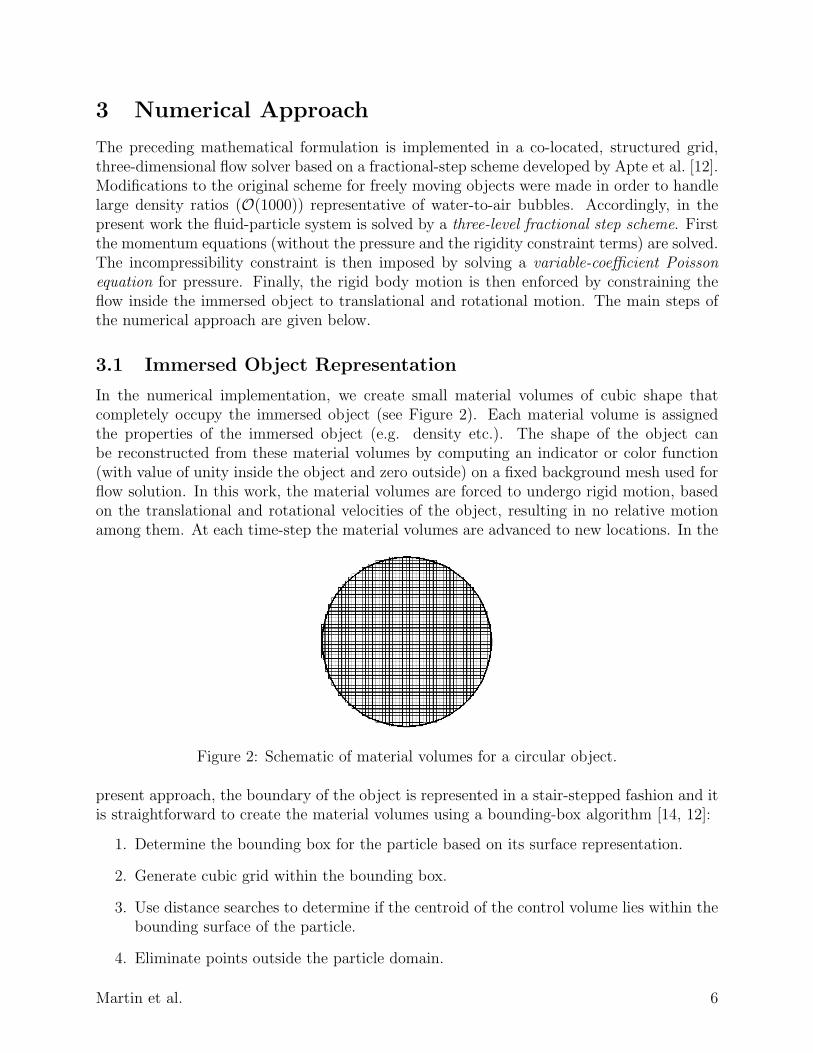
In the numerical implementation, we create small material volumes of cubic shape thatcompletely occupy the immersed object (see Figure 2). Each material volume is assignedthe properties of the immersed object (e.g. density etc.). The shape of the object canbe reconstructed from these material volumes by computing an indicator or color function(with value of unity inside the object and zero outside) on a fixed background mesh used forflow solution. In this work, the material volumes are forced to undergo rigid motion, basedon the translational and rotational velocities of the object, resulting in no relative motionamong them. At each time-step the material volumes are advanced to new locations. In the

Figure 2: Schematic of material volumes for a circular object.

present approach, the boundary of the object is represented in a stair-stepped fashion and itis straightforward to create the material volumes using a bounding-box algorithm [14, 12]:

1. Determine the bounding box for the particle based on its surface representation.

2. Generate cubic grid within the bounding box.

3. Use distance searches to determine if the centroid of the control volume lies within thebounding surface of the particle.

4. Eliminate points outside the particle domain.

Martin et al. 6

The total mass of the material volumes generated will be exactly equal to the mass of theparticle if the surface of the particle aligns with the grid. The stair-stepped surface repre-sentation, however, results in an error in the total mass of the material volumes compared tothe original shape. This error reduces with an increase in the total number of material vol-umes per object. A more complex grid generation process based on Delaunay triangulationcan be used to accurately represent the surface of the object by using standard body-fittedgrid generation tools. In the present work; however, we use sufficient number of materialvolumes to represent the object boundary and follow the stair-stepped approach owing toits simplicity.

3.2 Discretized Equations and Numerical Algorithm

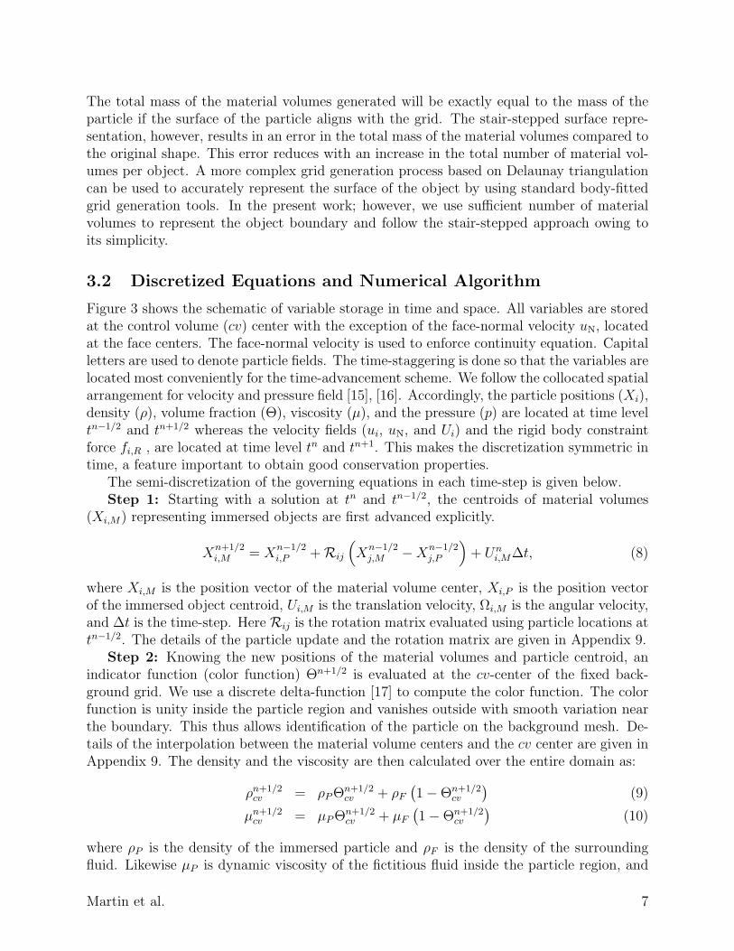
Figure 3 shows the schematic of variable storage in time and space. All variables are storedat the control volume (cv) center with the exception of the face-normal velocity uN, locatedat the face centers. The face-normal velocity is used to enforce continuity equation. Capitalletters are used to denote particle fields. The time-staggering is done so that the variables arelocated most conveniently for the time-advancement scheme. We follow the collocated spatialarrangement for velocity and pressure field [15], [16]. Accordingly, the particle positions (Xi),density (ρ), volume fraction (Θ), viscosity (µ), and the pressure (p) are located at time leveltn−1/2 and tn+1/2 whereas the velocity fields (ui, uN, and Ui) and the rigid body constraintforce fi,R , are located at time level tn and tn+1. This makes the discretization symmetric intime, a feature important to obtain good conservation properties.

The semi-discretization of the governing equations in each time-step is given below.Step 1: Starting with a solution at tn and tn−1/2, the centroids of material volumes

(Xi,M) representing immersed objects are first advanced explicitly.

Xn+1/2i,M = X

n−1/2i,P +Rij

(Xn−1/2j,M −Xn−1/2

j,P

)+ Un

i,M∆t, (8)

where Xi,M is the position vector of the material volume center, Xi,P is the position vectorof the immersed object centroid, Ui,M is the translation velocity, Ωi,M is the angular velocity,and ∆t is the time-step. Here Rij is the rotation matrix evaluated using particle locations attn−1/2. The details of the particle update and the rotation matrix are given in Appendix 9.

Step 2: Knowing the new positions of the material volumes and particle centroid, anindicator function (color function) Θn+1/2 is evaluated at the cv-center of the fixed back-ground grid. We use a discrete delta-function [17] to compute the color function. The colorfunction is unity inside the particle region and vanishes outside with smooth variation nearthe boundary. This thus allows identification of the particle on the background mesh. De-tails of the interpolation between the material volume centers and the cv center are given inAppendix 9. The density and the viscosity are then calculated over the entire domain as:

ρn+1/2cv = ρPΘn+1/2

cv + ρF(1−Θn+1/2

cv

)(9)

µn+1/2cv = µPΘn+1/2

cv + µF(1−Θn+1/2

cv

)(10)

where ρP is the density of the immersed particle and ρF is the density of the surroundingfluid. Likewise µP is dynamic viscosity of the fictitious fluid inside the particle region, and

Martin et al. 7

Figure 3: Schematic of the variable storage in time and space: (a) time-staggering, (b)three-dimensional variable storage, (c) cv and face notation, (d) index notation for a givenk-index in the z direction. The velocity fields (ui, uN) are staggered in time with respect tothe volume fraction (Θ), density (ρ), and particle position (Xi), the pressure field (p), andthe rigid body force (fi,R). All variables are collocated in space at the centroid of a controlvolume except the face-normal velocity uN which is stored at the centroid of the faces of thecontrol volume.

Martin et al. 8

µF is the dynamic viscosity of the surrounding fluid. For particles with specified motion(microvalves) µP is assumed equal to the fluid viscosity (µF ). For bubbles, appropriateviscosity of the air bubble is specified.

Step 3: Advance the momentum equations using the fractional step method [18]. First,obtain a predicted velocity field over the entire domain. We advance the velocity fieldfrom tn to tn+1. The predicted velocity fields may not satisfy the continuity or the rigidityconstraints. These are enforced later.

u∗i,cv − uni,cv

∆t+

1Vcv

∑faces of cv

u∗n+1/2i,face unNAface =

1

ρn+1/2cv

(1Vcv

∑faces of cv

τ∗n+1/2ij,face Nj,faceAface

)+ gi (11)

where gi is the gravitational acceleration, Vcv is the volume of the cv, Aface is the area of theface of a control volume, Nj,face is the face-normal vector and

u∗n+1/2i,face =

1

2

(uni,face + u∗i,face

);

τ∗n+1/2ij,face = µn+1/2

cv

[1

2

(∂uni∂xj

+∂u∗i∂xj

)+

(∂unj∂xi

)]face

In the above expressions, the velocities at the ‘face’ are obtained by using arithmetic averagesof the neighboring cvs attached to the face. For the viscous terms, the velocity gradients inthe direction of the momentum component are obtained implicitly using Crank-Nicholsonscheme. A centered discretization scheme is used for spatial gradients. Evaluation of thepressure gradients at the cv centers is explained below.

Step 4: Solve the variable coefficient Poisson equation for pressure:

1

∆t

∑faces of cv

u∗NAface =∑

faces of cv

1

ρn+1/2face

Afaceδp

δN

n+1/2

, (12)

where ρface is obtained using arithmetic averages of density in the neighboring cvs. Theface-normal velocity u∗N and the face-normal pressure gradient are obtained as:

u∗N =1

2(u∗i,nbr + u∗i,cv)Ni,face

δp

δN

n+1/2

=pn+1/2nbr − pn+1/2

cv

|scv,nbr|

where nbr represents neighboring cv associated with the face of the cv, and |scv,nbr| is thedistance between the two cvs. The variable-coefficient pressure equation is solved using aBi-Conjugate gradient algorithm [19].

Step 5: Reconstruct the pressure gradient at the cv centers using density and face-areaweighting first proposed by Ham & Young [20]

1

ρn+1/2cv

δp

δxi

n+1/2

=

∑faces of cv

1

ρn+1/2face

δpδN

n+1/2 ·~i|Ni,faceAface|∑faces of cv |Ni,faceAface|

(13)

Martin et al. 9

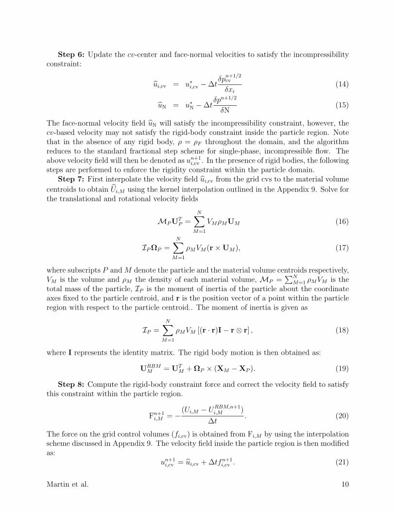
Step 6: Update the cv-center and face-normal velocities to satisfy the incompressibilityconstraint:

ui,cv = u∗i,cv −∆tδp

n+1/2cv

δxi(14)

uN = u∗N −∆tδpn+1/2

δN(15)

The face-normal velocity field uN will satisfy the incompressibility constraint, however, thecv-based velocity may not satisfy the rigid-body constraint inside the particle region. Notethat in the absence of any rigid body, ρ = ρF throughout the domain, and the algorithmreduces to the standard fractional step scheme for single-phase, incompressible flow. Theabove velocity field will then be denoted as un+1

i,cv . In the presence of rigid bodies, the followingsteps are performed to enforce the rigidity constraint within the particle domain.

Step 7: First interpolate the velocity field ui,cv from the grid cvs to the material volume

centroids to obtain Ui,M using the kernel interpolation outlined in the Appendix 9. Solve forthe translational and rotational velocity fields

MPUTP =

N∑M=1

VMρMUM (16)

IPΩP =N∑

M=1

ρMVM(r×UM), (17)

where subscripts P and M denote the particle and the material volume centroids respectively,VM is the volume and ρM the density of each material volume, MP =

∑NM=1 ρMVM is the

total mass of the particle, IP is the moment of inertia of the particle about the coordinateaxes fixed to the particle centroid, and r is the position vector of a point within the particleregion with respect to the particle centroid.. The moment of inertia is given as

IP =N∑

M=1

ρMVM [(r · r)I− r⊗ r] , (18)

where I represents the identity matrix. The rigid body motion is then obtained as:

URBMM = UT

M + ΩP × (XM −XP ). (19)

Step 8: Compute the rigid-body constraint force and correct the velocity field to satisfythis constraint within the particle region.

Fn+1i,M = −

(Ui,M − URBM,n+1i,M )

∆t. (20)

The force on the grid control volumes (fi,cv) is obtained from Fi,M by using the interpolationscheme discussed in Appendix 9. The velocity field inside the particle region is then modifiedas:

un+1i,cv = ui,cv + ∆tfn+1

i,cv . (21)

Martin et al. 10

4 Controller Design

Model-based control design requires a reduced order model of the flow dynamics that relatesindividual channel valve openings with the exit flow velocities for each channel. Whiledirect numerical simulations of the flow field produce the most accurate relationship betweenthese quantities, the computationally intensive nature of these simulations precludes theiruse in any real-time physical realization. However, many real-time control methodologieshave been developed to control linear, multiple-input, multiple-output (MIMO) systems.The development of a reduced order, linear MIMO model is therefore motivated both bythe ability of linear models to adequately represent nonlinear flow dynamics in certain flowregimes as well as the relative success of linear control methodologies in controlling nonlinearsystems.

4.1 System Identification

As a result, standard system identification techniques [21] are employed to produce a linearmodel of the flow dynamics which relates channel valve openings (inputs) to channel exitflow velocities (outputs). Specifically, an auto-regressive exogenous (ARX) model [22] of theflow dynamics is developed from direct numerical simulations of the flow regime, in whichchannel valve openings are varied in a prescribed fashion and the resulting output flowvelocities are recorded. While a linear, MIMO ARX model is developed, the relationshipbetween inputs and outputs in the ARX formulation is most easily illustrated for the single-input, single-output case. In this instance a linear difference equation relates the input andoutput

y(t) = −a1y(t− 1)− a2y(t− 2)− ...− anay(t− na) +

b1u(t− nk) + b2u(t− nk − 1) + ...+ bnbu(t− nk − nb + 1) (22)

where y(t) is the output, u(t) is the input, nk is the time delay, na is the number of poles,nb is the number of zeros plus one, and ai and bj are constants to be determined via theidentification process. The equation for the current output is therefore a function of bothvalues of the output and the input at previous sampling instants. The choice of how manyprevious input and output values to retain is driven by the model validation procedure, inwhich the output prediction of the model is compared to the results obtained from directnumerical simulations of the flow for data not utilized in the identification process. In themulti-variable case, the coefficients ai and bi become no×no and no×ni matrices, respectively,where no and ni represent the number of model outputs and inputs.

System identification is conducted following the procedure presented in [22]. Uncontrolledsimulations are utilized to determine the system settling time, which informs the choice ofboth the sampling interval and the duration of the identification tests. Identification testsare subsequently conducted via numerical simulations of the flow field, in which channelvalve angles are randomly varied to excite all modes of the flow dynamics. Flow velocitiesat the exit of each channel are recorded and this output data, in conjunction with therecorded variation of the input valve orientations, is processed within the Matlab systemidentification toolbox to produce multiple linear ARX models of varying order. Models

Martin et al. 11

are validated against numerical simulation data not used in the identification procedure.Channel exit flow velocities are generated by each model from the prescribed variation ofthe input valves used to produce the validation data set. These velocities are compared tothose obtained by direct numerical simulation of the flow field. Model selection is governedby output accuracy, as balanced with model simplicity. The selected linear, MIMO systemmodel is subsequently employed as a substitute for the actual flow dynamics in the modelpredictive controller design.

4.2 Model Predictive Control

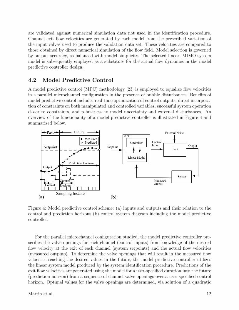
A model predictive control (MPC) methodology [23] is employed to equalize flow velocitiesin a parallel microchannel configuration in the presence of bubble disturbances. Benefits ofmodel predictive control include: real-time optimization of control outputs, direct incorpora-tion of constraints on both manipulated and controlled variables, successful system operationcloser to constraints, and robustness to model uncertainty and external disturbances. Anoverview of the functionality of a model predictive controller is illustrated in Figure 4 andsummarized below.

Figure 4: Model predictive control scheme: (a) inputs and outputs and their relation to thecontrol and prediction horizons (b) control system diagram including the model predictivecontroller.

For the parallel microchannel configuration studied, the model predictive controller pre-scribes the valve openings for each channel (control inputs) from knowledge of the desiredflow velocity at the exit of each channel (system setpoints) and the actual flow velocities(measured outputs). To determine the valve openings that will result in the measured flowvelocities reaching the desired values in the future, the model predictive controller utilizesthe linear system model produced by the system identification procedure. Predictions of theexit flow velocities are generated using the model for a user-specified duration into the future(prediction horizon) from a sequence of channel valve openings over a user-specified controlhorizon. Optimal values for the valve openings are determined, via solution of a quadratic

Martin et al. 12

programming problem, over the control horizon such that a cost function involving the devi-ation from the desired setpoints is minimized over the prediction horizon. Once the optimalsequence of valve openings is determined, only the first set of openings are provided tothe flow solver (plant). At the next sampling instant, the resulting exit flow velocities aremeasured and sent to the model predictive control scheme. Utilizing this new informationregarding the actual flow velocities achieved as a result of the valve openings, as opposed tothose predicted by the linear model, the process repeats.

Realization of the model predictive control design is achieved by through the Matlabmodel predictive control toolbox. The system model, control horizon, prediction horizon,cost function structure and associated weighting matrices, setpoint values and the measuredoutputs are input into the MPC toolbox. The quadratic programming problem is solvedwithin the toolbox to produce the channel valve openings utilized by the flow solver. Theresulting strategy is computationally lightweight, enabling future physical implementationwith small microcontrollers.

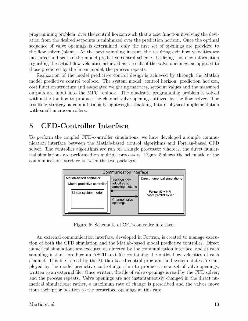
5 CFD-Controller Interface

To perform the coupled CFD-controller simulations, we have developed a simple commu-nication interface between the Matlab-based control algorithms and Fortran-based CFDsolver. The controller algorithms are run on a single processor; whereas, the direct numer-ical simulations are performed on multiple processors. Figure 5 shows the schematic of thecommunication interface between the two packages.

Figure 5: Schematic of CFD-controller interface.

An external communication interface, developed in Fortran, is created to manage execu-tion of both the CFD simulation and the Matlab-based model predictive controller. Directnumerical simulations are executed as directed by the communication interface, and at eachsampling instant, produce an ASCII text file containing the outlet flow velocities of eachchannel. This file is read by the Matlab-based control program, and system states are em-ployed by the model predictive control algorithm to produce a new set of valve openings,written to an external file. Once written, the file of valve openings is read by the CFD solver,and the process repeats. Valve openings are not instantaneously changed in the direct nu-merical simulations; rather, a maximum rate of change is prescribed and the valves movefrom their prior position to the prescribed openings at this rate.

Martin et al. 13

The direct numerical simulations mainly govern the total simulation time mainly due tothe details of the flow captured. The Matlab-based controller takes negligible amount oftime compared to CFD. This framework is efficient and is applicable to several other physicsproblems requiring coupling of CFD and model-predictive control.

6 Validation cases

The numerical formulation together with the control algorithm are first used to performbasic validation and verification studies. The numerical test cases were chosen to validatethe basic incompressible flow algorithm applied to high-aspect ratio channel flows, flowdeveloped by objects undergoing specified motion to test the capability of the solver to handlemoving microvalves, motion of freely moving particles and bubbles, and finally testing of thecoupled CFD-control algorithm. Accordingly, the following tests are performed: (i) singlephase incompressible flow in a high-aspect ratio microchannel at different Reynolds numberscorresponding to the experimental data of Qu et al. [24], (ii) flow over a fixed cylinder atdifferent Reynolds number, (iii) flow developed by an oscillating sphere corresponding toexperiments by [25], (iv) rising of a small bubble in an inclined channel corresponding toexperiments by [26], and (v) equalizing mass-flow rates in parallel microchannels using model-predictive control. After these extensive validation studies, the coupled solver is applied tomitigate flow maldistribution in parallel microchannels.

6.1 Microchannel channel case

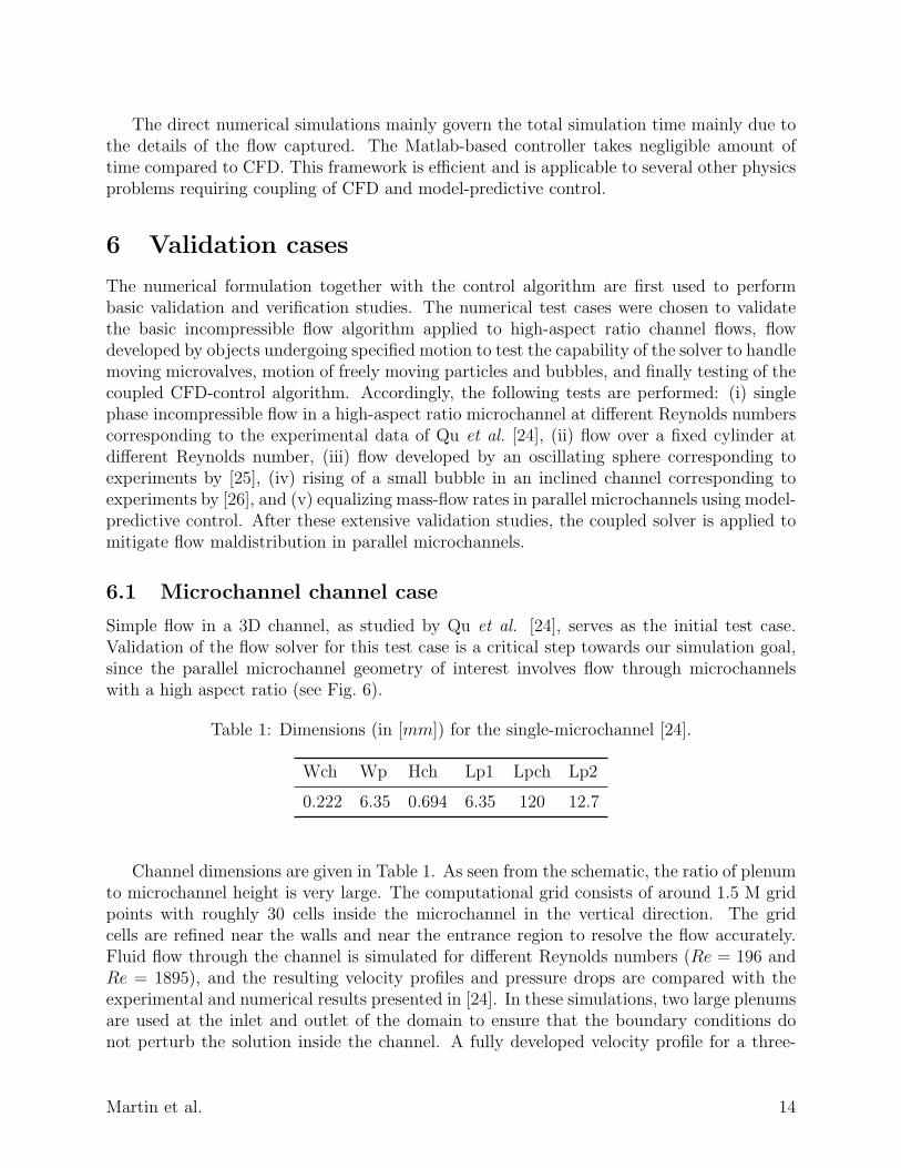
Simple flow in a 3D channel, as studied by Qu et al. [24], serves as the initial test case.Validation of the flow solver for this test case is a critical step towards our simulation goal,since the parallel microchannel geometry of interest involves flow through microchannelswith a high aspect ratio (see Fig. 6).

Table 1: Dimensions (in [mm]) for the single-microchannel [24].

Wch Wp Hch Lp1 Lpch Lp2

0.222 6.35 0.694 6.35 120 12.7

Channel dimensions are given in Table 1. As seen from the schematic, the ratio of plenumto microchannel height is very large. The computational grid consists of around 1.5 M gridpoints with roughly 30 cells inside the microchannel in the vertical direction. The gridcells are refined near the walls and near the entrance region to resolve the flow accurately.Fluid flow through the channel is simulated for different Reynolds numbers (Re = 196 andRe = 1895), and the resulting velocity profiles and pressure drops are compared with theexperimental and numerical results presented in [24]. In these simulations, two large plenumsare used at the inlet and outlet of the domain to ensure that the boundary conditions donot perturb the solution inside the channel. A fully developed velocity profile for a three-

Martin et al. 14

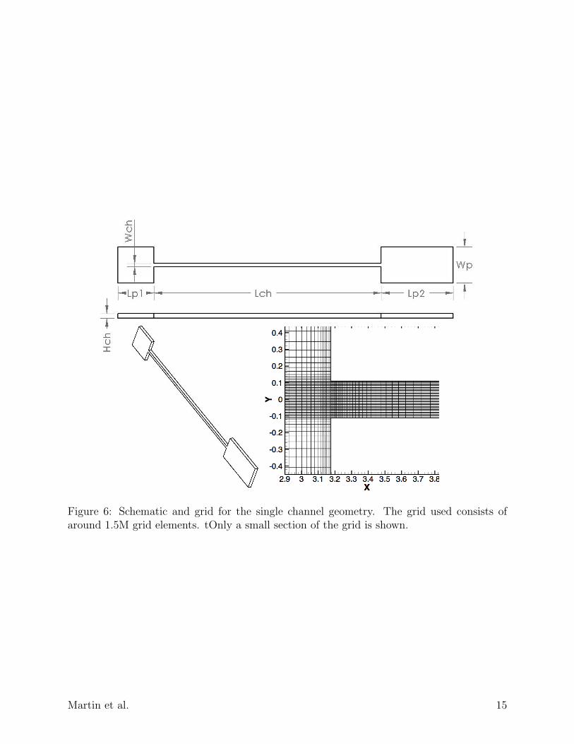
Figure 6: Schematic and grid for the single channel geometry. The grid used consists ofaround 1.5M grid elements. tOnly a small section of the grid is shown.

Martin et al. 15

dimensional rectangular channel [24] is applied at the inlet of the domain and data is onlycollected after the flow in the channel reaches steady state.

Y

U

0 50 100 150 2000

0.2

0.4

0.6

0.8

1

1.2

1.4

(a) Re = 196, x′ = 1 cm

YU

50 100 150 2000

2

4

6

8

10

(b) Re = 1895, x′ = 1 cm

Y

U

50 100 150 2000

2

4

6

8

10

(c) Re = 1895, x′ = 10 cm

Figure 7: Velocity profiles in the center plane of the channel taken at x′ = 1cm and x′ = 10cmfrom the entrance of the channel. • shows the experimental data, − − − the numericalsimulation from [24] and — the present study. The velocity is expressed in [m/s] and the ylocation in [µm].

X

Uc

0 0.02 0.04 0.06 0.08 0.1 0.120

2

4

6

8

10

12

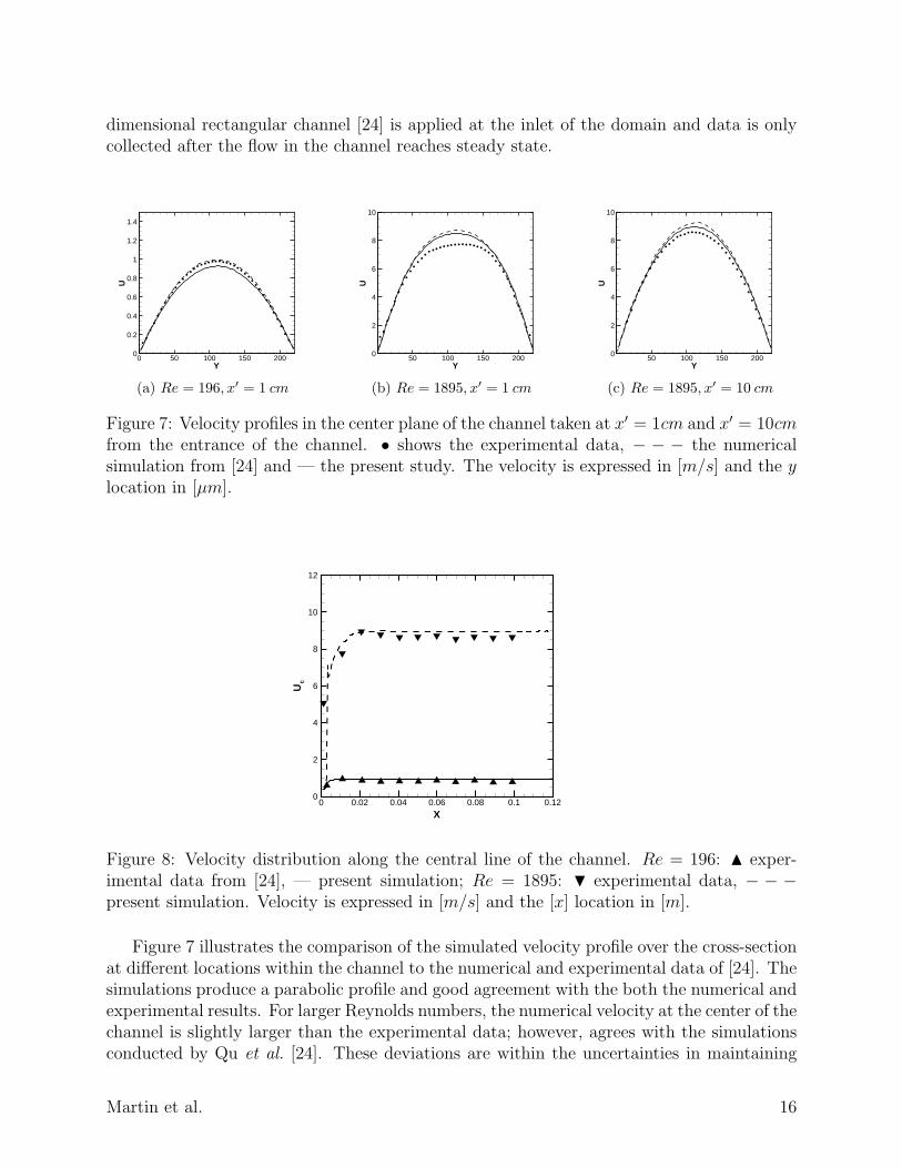
Figure 8: Velocity distribution along the central line of the channel. Re = 196: N exper-imental data from [24], — present simulation; Re = 1895: H experimental data, − − −present simulation. Velocity is expressed in [m/s] and the [x] location in [m].

Figure 7 illustrates the comparison of the simulated velocity profile over the cross-sectionat different locations within the channel to the numerical and experimental data of [24]. Thesimulations produce a parabolic profile and good agreement with the both the numerical andexperimental results. For larger Reynolds numbers, the numerical velocity at the center of thechannel is slightly larger than the experimental data; however, agrees with the simulationsconducted by Qu et al. [24]. These deviations are within the uncertainties in maintaining

Martin et al. 16

constant flow rates as well as velocity measurements. As illustrated in Figure 8, the velocityalong the center line of the channel, for the length of the channel, shows very good agreementwith the experimental data.

Table 2: Comparison between computed and theoretical pressure drops at different Reynoldsnumbers.

Pressure Drop [bar]

Rech DNS (with plenum) DNS (without plenum) Theory (without plenum)196 0.189 0.195 0.201021 1.09 1.06 1.041895 1.33 1.87 1.93

Table 2 presents the comparison of numerically obtained pressure drop inside the mi-crochannel with the theoretical pressure drop in a square microchannel (excluding theplenums). A good agreement is achieved for low Reynolds number (up to Rech = 1021).For Rech = 1895 the pressure drop is under-predicted by the simulation. This is attributedto the effects of sudden changes in aspect ratios near the inlet and outlet plenums. Flowseparations are possible near the entrance, modifying the flow evolution to fully developedvelocity profile and thus affecting the overall pressure drop. To test the accuracy of the solver,we have also simulated flow through the microchannel duct (without the plenums) with uni-form inlet on a grid similar to the grid used for the case with plenums. The pressure-dropvalues for the same mass-flow rates are shown in Table 2 and agree well with the theoreticalestimates.

6.2 Flow induced by an oscillating cylinder

Simulation of a periodic oscillating cylinder in a fluid at rest has often been used to test theaccuracy of immersed boundary techniques, and serves as our second test case. Numericalsimulation results are validated against those of [27] as well as experimental data availablefrom [25].

Two non-dimensional numbers characterize a periodic oscillating cylinder: the Reynoldsnumber Re = Umd/ν and the Keulegan-Carpenter number KC = Um/fd, where Um =0.01m/s is the maximum velocity of the cylinder, f = 0.2Hz the frequency of the oscillations,d = 0.01m is the diameter of the cylinder and ν the kinematic viscosity. The position of thecylinder in the x-direction is defined by the equation:

xp(t) = −Ap sinωt (23)

where xp(t) is the location of the centroid of the cylinder in the x-direction and Ap isthe maximum amplitude of the oscillations. Because the oscillation frequency is given byω = 2πf , the Keulegan-Carpenter number can be rewritten as KC = 2πAp/d. Simulationsare conducted with Red = 100 and KC = 5, as in [27]. The computational domain is

Martin et al. 17

u/Um

y/D

-1 -0.5 0 0.5 1 1.5

-1

-0.5

0

0.5

1

(a) ωt = 180u/Um

y/D

-1 -0.5 0 0.5 1 1.5

-1

-0.5

0

0.5

1

(b) ωt = 210u/Um

y/D

-0.4 -0.2 0 0.2 0.4

-1

-0.5

0

0.5

1

(c) ωt = 330

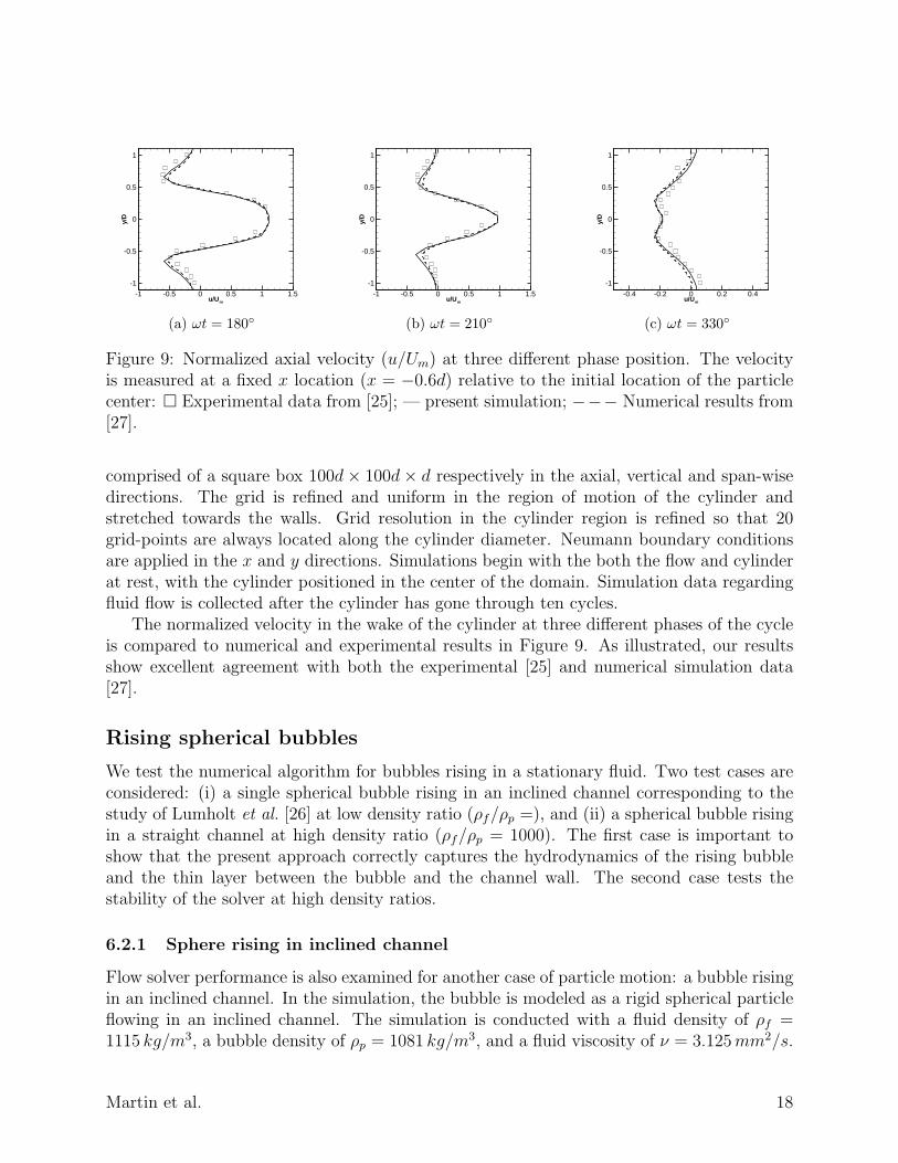
Figure 9: Normalized axial velocity (u/Um) at three different phase position. The velocityis measured at a fixed x location (x = −0.6d) relative to the initial location of the particlecenter: Experimental data from [25]; — present simulation; −−− Numerical results from[27].

comprised of a square box 100d× 100d× d respectively in the axial, vertical and span-wisedirections. The grid is refined and uniform in the region of motion of the cylinder andstretched towards the walls. Grid resolution in the cylinder region is refined so that 20grid-points are always located along the cylinder diameter. Neumann boundary conditionsare applied in the x and y directions. Simulations begin with the both the flow and cylinderat rest, with the cylinder positioned in the center of the domain. Simulation data regardingfluid flow is collected after the cylinder has gone through ten cycles.

The normalized velocity in the wake of the cylinder at three different phases of the cycleis compared to numerical and experimental results in Figure 9. As illustrated, our resultsshow excellent agreement with both the experimental [25] and numerical simulation data[27].

Rising spherical bubbles

We test the numerical algorithm for bubbles rising in a stationary fluid. Two test cases areconsidered: (i) a single spherical bubble rising in an inclined channel corresponding to thestudy of Lumholt et al. [26] at low density ratio (ρf/ρp =), and (ii) a spherical bubble risingin a straight channel at high density ratio (ρf/ρp = 1000). The first case is important toshow that the present approach correctly captures the hydrodynamics of the rising bubbleand the thin layer between the bubble and the channel wall. The second case tests thestability of the solver at high density ratios.

6.2.1 Sphere rising in inclined channel

Flow solver performance is also examined for another case of particle motion: a bubble risingin an inclined channel. In the simulation, the bubble is modeled as a rigid spherical particleflowing in an inclined channel. The simulation is conducted with a fluid density of ρf =1115 kg/m3, a bubble density of ρp = 1081 kg/m3, and a fluid viscosity of ν = 3.125mm2/s.

Martin et al. 18

The Reynolds number ReStokesp based on the Stokes settling velocity W is defined as :

ReStokesp =2aW

ν=

4a3

9ν2|ρpρf− 1|g (24)

where g = 9.82 m/s2 is the gravitational acceleration, and a = 2 mm is the diameter of theparticle. The channel is inclined at an angle of 8.23 with the vertical. This is simulated byadding components of gravitational forces in the horizontal and vertical directions.

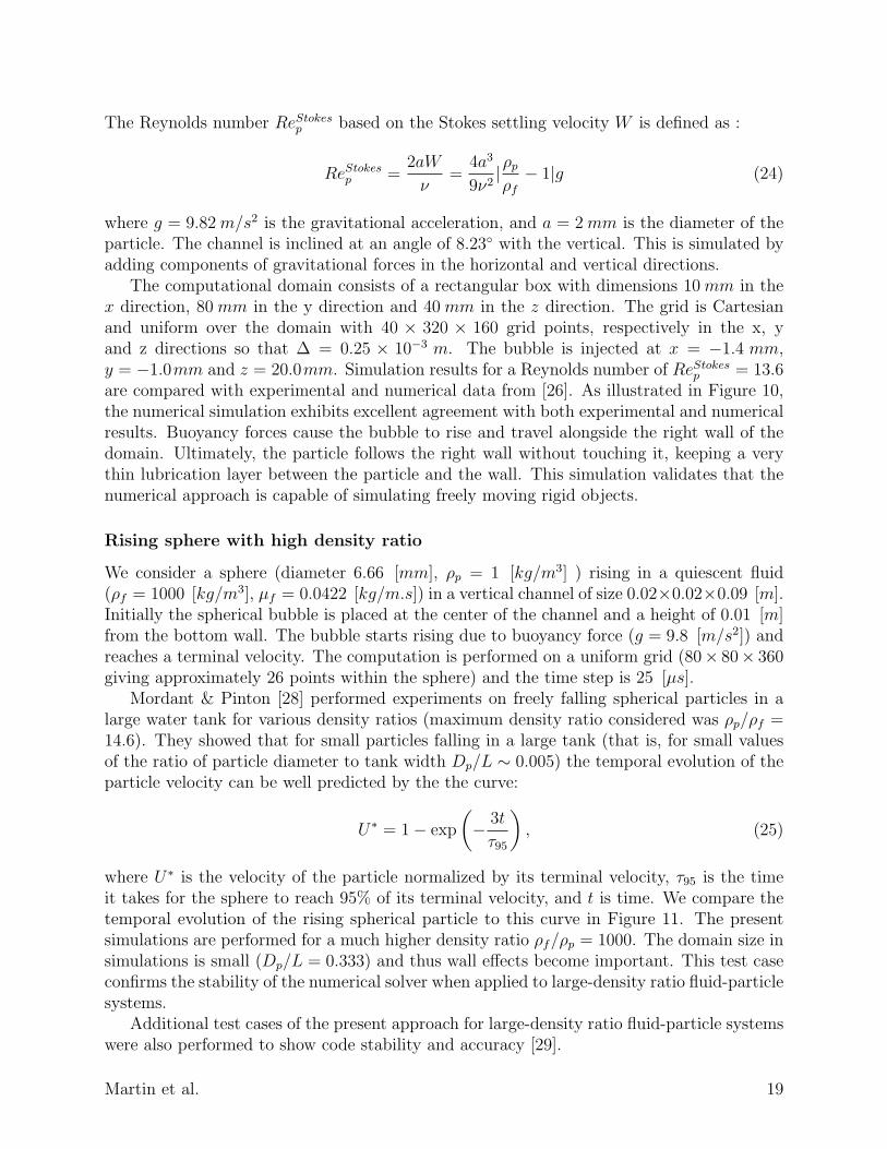
The computational domain consists of a rectangular box with dimensions 10 mm in thex direction, 80 mm in the y direction and 40 mm in the z direction. The grid is Cartesianand uniform over the domain with 40 × 320 × 160 grid points, respectively in the x, yand z directions so that ∆ = 0.25 × 10−3 m. The bubble is injected at x = −1.4 mm,y = −1.0mm and z = 20.0mm. Simulation results for a Reynolds number of ReStokesp = 13.6are compared with experimental and numerical data from [26]. As illustrated in Figure 10,the numerical simulation exhibits excellent agreement with both experimental and numericalresults. Buoyancy forces cause the bubble to rise and travel alongside the right wall of thedomain. Ultimately, the particle follows the right wall without touching it, keeping a verythin lubrication layer between the particle and the wall. This simulation validates that thenumerical approach is capable of simulating freely moving rigid objects.

Rising sphere with high density ratio

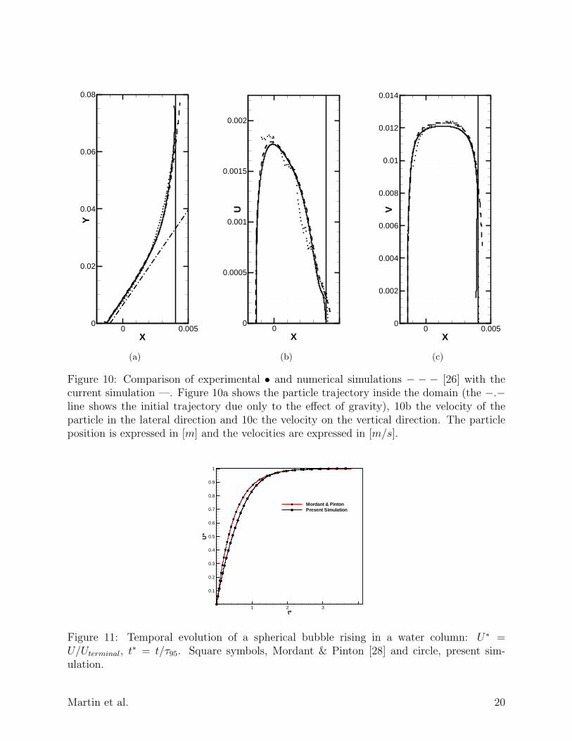
We consider a sphere (diameter 6.66 [mm], ρp = 1 [kg/m3] ) rising in a quiescent fluid(ρf = 1000 [kg/m3], µf = 0.0422 [kg/m.s]) in a vertical channel of size 0.02×0.02×0.09 [m].Initially the spherical bubble is placed at the center of the channel and a height of 0.01 [m]from the bottom wall. The bubble starts rising due to buoyancy force (g = 9.8 [m/s2]) andreaches a terminal velocity. The computation is performed on a uniform grid (80× 80× 360giving approximately 26 points within the sphere) and the time step is 25 [µs].

Mordant & Pinton [28] performed experiments on freely falling spherical particles in alarge water tank for various density ratios (maximum density ratio considered was ρp/ρf =14.6). They showed that for small particles falling in a large tank (that is, for small valuesof the ratio of particle diameter to tank width Dp/L ∼ 0.005) the temporal evolution of theparticle velocity can be well predicted by the the curve:

U∗ = 1− exp

(− 3t

τ95

), (25)

where U∗ is the velocity of the particle normalized by its terminal velocity, τ95 is the timeit takes for the sphere to reach 95% of its terminal velocity, and t is time. We compare thetemporal evolution of the rising spherical particle to this curve in Figure 11. The presentsimulations are performed for a much higher density ratio ρf/ρp = 1000. The domain size insimulations is small (Dp/L = 0.333) and thus wall effects become important. This test caseconfirms the stability of the numerical solver when applied to large-density ratio fluid-particlesystems.

Additional test cases of the present approach for large-density ratio fluid-particle systemswere also performed to show code stability and accuracy [29].

Martin et al. 19

X

Y

0 0.0050

0.02

0.04

0.06

0.08

(a)

X

U

00

0.0005

0.001

0.0015

0.002

(b)

X

V

0 0.0050

0.002

0.004

0.006

0.008

0.01

0.012

0.014

(c)

Figure 10: Comparison of experimental • and numerical simulations − − − [26] with thecurrent simulation —. Figure 10a shows the particle trajectory inside the domain (the −.−line shows the initial trajectory due only to the effect of gravity), 10b the velocity of theparticle in the lateral direction and 10c the velocity on the vertical direction. The particleposition is expressed in [m] and the velocities are expressed in [m/s].

t*

U*

1 2 3

0.1

0.2

0.3

0.4

0.5

0.6

0.7

0.8

0.9

1

Mordant & PintonPresent Simulation

Figure 11: Temporal evolution of a spherical bubble rising in a water column: U∗ =U/Uterminal, t

∗ = t/τ95. Square symbols, Mordant & Pinton [28] and circle, present sim-ulation.

Martin et al. 20

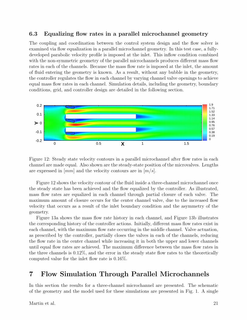
6.3 Equalizing flow rates in a parallel microchannel geometry

The coupling and coordination between the control system design and the flow solver isexamined via flow equalization in a parallel microchannel geometry. In this test case, a fully-developed parabolic velocity profile is imposed at the inlet. This inflow condition combinedwith the non-symmetric geometry of the parallel microchannels produces different mass flowrates in each of the channels. Because the mass flow rate is imposed at the inlet, the amountof fluid entering the geometry is known. As a result, without any bubble in the geometry,the controller regulates the flow in each channel by varying channel valve openings to achieveequal mass flow rates in each channel. Simulation details, including the geometry, boundaryconditions, grid, and controller design are detailed in the following section.

X

Y

0 0.5 1 1.5-0.2

-0.1

0

0.1

0.2 1.91.711.521.331.140.950.760.570.380.190

Figure 12: Steady state velocity contours in a parallel microchannel after flow rates in eachchannel are made equal. Also shown are the steady-state position of the microvalves. Lengthsare expressed in [mm] and the velocity contours are in [m/s].

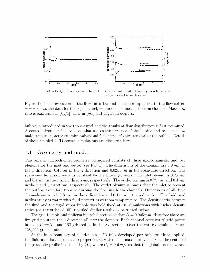
Figure 12 shows the velocity contour of the fluid inside a three-channel microchannel oncethe steady state has been achieved and the flow equalized by the controller. As illustrated,mass flow rates are equalized in each channel through partial closure of each valve. Themaximum amount of closure occurs for the center channel valve, due to the increased flowvelocity that occurs as a result of the inlet boundary condition and the asymmetry of thegeometry.

Figure 13a shows the mass flow rate history in each channel, and Figure 13b illustratesthe corresponding history of the controller actions. Initially, different mass flow rates exist ineach channel, with the maximum flow rate occurring in the middle channel. Valve actuation,as prescribed by the controller, partially closes the valves in each of the channels, reducingthe flow rate in the center channel while increasing it in both the upper and lower channelsuntil equal flow rates are achieved. The maximum difference between the mass flow rates inthe three channels is 0.12%, and the error in the steady state flow rates to the theoreticallycomputed value for the inlet flow rate is 0.16%.

7 Flow Simulation Through Parallel Microchannels

In this section the results for a three-channel microchannel are presented. The schematicof the geometry and the model used for these simulations are presented in Fig. 1. A single

Martin et al. 21

time

mas

sflo

wra

te

0 0.5 1 1.5 2 2.50.7

0.75

0.8

0.85

0.9

(a) Velocity history in each channel

time

cont

rolle

rco

mm

and

angl

eap

plie

d

1 2 3 4 50

0.05

0.1

0.15

0.2

0.25

0.3

0.35

0

2

4

6

8

10

12

14

top channel

middle channel

bottom channel

(b) Controller output history correlated withangle applied to each valve.

Figure 13: Time evolution of the flow rates 13a and controller input 13b to the flow solver:−−− shows the data for the top channel; — middle channel; -.- bottom channel. Mass flowrate is expressed in [kg/s], time in [ms] and angles in degrees.

bubble is introduced in the top channel and the resultant flow distribution is first examined.A control algorithm is developed that senses the presence of the bubble and resultant flowmaldistribution, activates microvalves and facilitates effective removal of the bubble. Detailsof these coupled CFD-control simulations are discussed here.

7.1 Geometry and model

The parallel microchannel geometry considered consists of three microchannels, and twoplenums for the inlet and outlet (see Fig. 1). The dimensions of the domain are 0.8 mm inthe x direction, 0.4 mm in the y direction and 0.025 mm in the span-wise direction. Thespan-wise dimension remains constant for the entire geometry. The inlet plenum is 0.25mmand 0.4mm in the x and y directions, respectively. The outlet plenum is 0.75mm and 0.4mmin the x and y directions, respectively. The outlet plenum is longer than the inlet to preventthe outflow boundary from perturbing the flow inside the channels. Dimensions of all threechannels are equal: 0.8mm in the x direction and 0.1mm in the y direction. The fluid usedin this study is water with fluid properties at room temperature. The density ratio betweenthe fluid and the rigid vapor bubble was held fixed at 10. Simulations with higher densityratios (on the order of 100) revealed similar results as presented below.

The grid is cubic and uniform in each direction so that ∆ = 0.005mm, therefore there arefive grid points in the z direction all over the domain. Each channel contains 20 grid-pointsin the y direction and 160 grid-points in the x direction. Over the entire domain there are128, 000 grid-points.

At the inlet boundary of the domain a 2D fully-developed parabolic profile is applied,the fluid used having the same properties as water. The maximum velocity at the center ofthe parabolic profile is defined by 3

2Up where Up = 0.6m/s so that the global mass flow rate

Martin et al. 22

entering the computational domain is m = 2.4mg/s.

7.2 System identification and controller development

The system settling time in response to a step change in a valve position was numericallydetermined as approximately 0.8ms, which was the time required for the channel flow veloc-ities to reach 98% of their steady state values. A sampling interval of one twentieth of thesettling time, or .04ms, was chosen for both the identification tests and the control design.A generalized binary noise (GBN) signal was generated to prescribe the closure of each ofthe valves between fully open and 50% closed for the system identification test. The GBNsignal was created with a mean switching time of one third the settling time and a minimumswitching time equal to the sampling rate. The duration of the test was twelve times thesettling time, or 9.6ms.

Input and output data generated by the numerical system identification test was pro-cessed in the MATLAB system identification toolbox to produce ARX models of varyingcomplexity. Model validation was performed for each model, with model quality judged bya ”best fit” criteria

Best F it =

(1− ‖y − y‖‖y − y‖

)× 100 (26)

where y is the measured output, y is the predicted output and y is mean of the measuredoutput. A model has a perfect Best Fit value of 100% if y is equal to y. A best fit valueof zero represents a fit which is no better than picking a constant value of y for the modeloutput. A model with three poles, two zeros and one delay produced best fit values of 86.5%,87.6% and 83.7%, for channels one, two and three, respectively. Models of lower order weresignificantly less accurate while higher order models were only marginally more accurate.The model identified by this process, and subsequently utilized in the controller design, was

Iy(t) = −

−2.09 −0.91 −0.74−1.70 −3.00 −1.873.13 3.21 1.96

y(t− 1)−

2.15 1.92 1.69−1.00 −0.72 −0.76−0.99 −1.04 −0.77

y(t− 2)−

−1.82 −1.85 −1.791.99 2.04 1.92−0.03 −0.05 0.01

y(t− 3) +

0.05 −0.02 −0.02−0.02 0.05 −0.02−0.03 −0.03 0.04

u(t− 1) +

0.01 −0.03 −0.01−0.01 0.03 −0.02−0.01 −0.00 0.02

u(t− 2) +

−0.02 0.02 0.010.01 −0.04 0.010.01 0.02 −0.02

u(t− 3) (27)

where y(t) = [y1(t) y2(t) y3(t)]T represents the flow velocity in each channel and u(t) =[u1(t) u2(t) u3(t)]T represents the valve closure for each channel.

Controller design required specification of the control horizon, prediction horizon, as wellas the cost function form and associated weighting parameters. In this study, a quadraticcost function was constructed in terms of a vector of valve positions, a vector comprisedof the change in the valve positions in one sampling period, and a vector representing thedifference between the exit flow rates and the desired values. Selection of the values in theweighting matrices of the cost function provided a means to balance the magnitude and rate

Martin et al. 23

of the valve closures with the attainment of the desired exit flow rates. Initial values for thecontrol horizon, prediction horizon and weighting matrices were computed via the tuningstrategy detailed in [30]. These parameters were subsequently refined based upon simulationresults of the controlled performance. Final values utilized in the simulation results arepresented in Table 3.

Table 3: Control parameters used for controller design and system ID tests.

Control ParametersControl Horizon 5 sampling periods 0.2 msPrediction Horizon 10 sampling periods 0.4 msValve Position Weighting Matrix Diagonal 3 x 3 matrix, 0.001 on diagonalValve Rate Weighting Matrix Diagonal 3 x 3 matrix, 1.0 on diagonalOutput Error Weighting Matrix Diagonal 3 x 3 matrix, 10 on diagonalValve Opening Constraint Constrained to remain between 0 and 1Valve Rate Constraint Constrained to remain within -0.15 and 0.15

7.3 Effect of a single bubble on the flow distribution

First, the effect of a single bubble, present in the top channel of the three-channel geometry,on the flow distribution is investigated. A 60 µm bubble is introduced in the top channel,close to the bottom side of the channel wall. The bubble plugs 60% of the channel height.The bubble is held fixed at this location and its effect on the flow distribution and pressuredrop are presented below. In this work, we do not simulate the physics of bubble nucleationand bubble growth. Instead, a bubble is introduced initially and held fixed. This representsa practical situation wherein the surface tension and viscous forces on the bubble are greaterthan the hydrodynamic forces, and the bubble remains attached to one side of the channelwall.

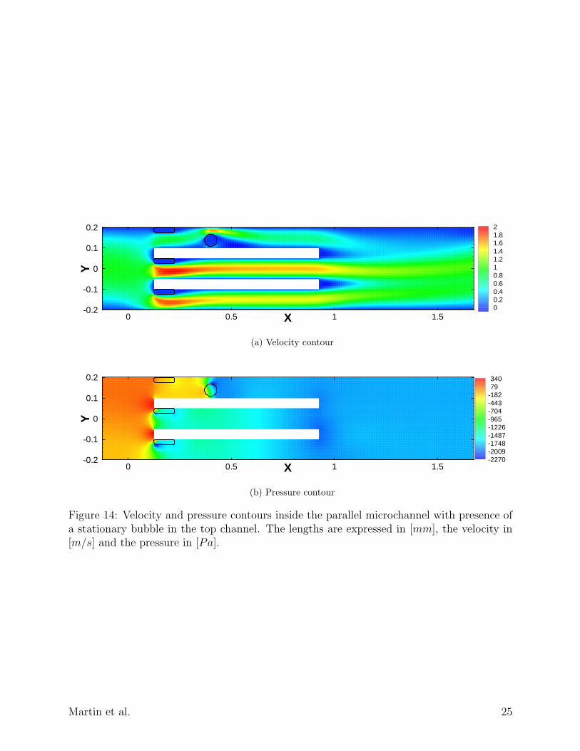
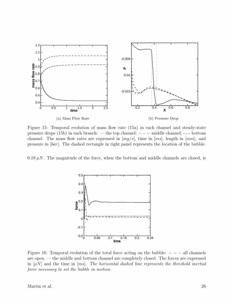
Figures 14a-b show contours of axial flow velocity and pressure inside the parallel mi-crochannel in the presence of a bubble in the top channel. For this configuration the mi-crovalves are completely open and controller is not activated, and the flow maldistributionis clearly visible. Figure 15a shows the history of flow rates in each channel after the bubbleis injected into the top channel, whereas Fig. 15b shows the steady state pressure drop ineach branch of the microchannel in the presence of the bubble, indicating higher pressuredrop in the top channel.

Next, we estimate the range of forces acting on the bubble held fixed in the top channel byvarying the microvalve configurations. We consider two extreme cases: (a) all microvalvesare completely open, and (b) the middle and bottom channel are completely closed bymicrovalves. In the first case, majority of the flow goes through the middle and bottombranches, whereas in the latter case all flow goes through the top channel. Figure 16 showsthe time history of the forces on the bubble in these two extreme configurations. It is foundthat when the bottom and middle channels are completely closed, the entire inflow goesthrough the top channel, increasing the hydrodynamic forces on the bubble. The rangeof the forces applied to the bubble in these extreme configurations vary from 0.013 µN to

Martin et al. 24

X

Y

0 0.5 1 1.5-0.2

-0.1

0

0.1

0.2 21.81.61.41.210.80.60.40.20

(a) Velocity contour

X

Y

0 0.5 1 1.5-0.2

-0.1

0

0.1

0.2 34079

-182-443-704-965-1226-1487-1748-2009-2270

(b) Pressure contour

Figure 14: Velocity and pressure contours inside the parallel microchannel with presence ofa stationary bubble in the top channel. The lengths are expressed in [mm], the velocity in[m/s] and the pressure in [Pa].

Martin et al. 25

time

mas

sflo

wra

te

0 0.5 1 1.5 2 2.5

0.4

0.5

0.6

0.7

0.8

0.9

1

1.1

1.2

(a) Mass Flow Rate

X

P

0.2 0.4 0.6 0.8

-0.015

-0.01

-0.005

(b) Pressure Drop

Figure 15: Temporal evolution of mass flow rate (15a) in each channel and steady-statepressure drops (15b) in each branch: — the top channel; −−− middle channel; -.-.- bottomchannel. The mass flow rates are expressed in [mg/s], time in [ms], length in [mm], andpressure in [bar]. The dashed rectangle in right panel represents the location of the bubble.

0.19 µN . The magnitude of the force, when the bottom and middle channels are closed, is

Figure 16: Temporal evolution of the total force acting on the bubble: − − − all channelsare open, — the middle and bottom channel are completely closed. The forces are expressedin [µN ] and the time in [ms]. The horizontal dashed line represents the threshold inertialforce necessary to set the bubble in motion.

Martin et al. 26

larger than the forces necessary to hold the bubble fixed, estimated based on the surfacetension forces, and thus the bubble can be removed by increasing mass flow rate in the topchannel. Without any actuation (i.e. all valves are completely open), the hydrodynamicforce on the bubble is insufficient to overcome the estimated surface tension forces, and thusthe bubble will remain fixed inside the top channel. The goal of the controller then is tofirst detect flow maldistribution and then activate microvalves such that the flow rate insidethe top channel is increased sufficiently to remove the bubble. This is achieved by slowlyactivating the microvalves in the middle and the bottom channel.

7.4 Coupled CFD-Controller Simulations

The model predictive control algorithm developed above is applied to mitigate flow maldis-tribution due to presence of bubbles in branches of parallel microchannels shown in Fig. 1 .Two cases are investigated to show the effectiveness of the controlled simulations: (i) pres-ence of a single bubble in the top channel, (ii) presence of one bubble in the top and bottomchannels. The history of the controller commands, evolution of the flow rates in each branch,and the trajectory of the bubble are presented below.

7.4.1 Single bubble simulation

We start with a steady-state solution for the three-channel geometry (see Fig. 1) with valveconfigurations set such that flow rates are equalized in branch of the channel. A single bubbleof diameter 60 µm, blocking the upper channel 60% is then introduced in the upper channel.The controller sensor and actuator are activated to first sense the flow maldistribution andthen provide inputs to the microvalves to regulate the flow rates in each channel such thatthe bubble is effectively removed.

As a sensor, we monitor the flow rates at the exit of each branch of the microchannel.Figure 17 shows the history of the mass flow rates in each branch of the microchannel startingwith initial equal rates. With the presence of the bubble in the top branch, the mass-flowrate in the top channel decreases whereas those in the bottom and middle channels increase.This disparity in the flow rates is detected by the sensor, and the controller provides a seriesof commands to each microvalve such that equal flow rates are restored in each channel.

Figures 18a-c provide the temporal history of the controller command, the location andvelocities of the bubble. As the sensor senses flow maldistribution, it starts to close themiddle and bottom channels, thus increasing the flow rate in the top channel. This increasein flow increases the hydrodynamic forces on the bubble and the bubble is set in motionas soon as the hydrodynamic force exceeds a pre-calculated resistive force (due to surfacetension forces) on the bubble. Once in motion, the bubble quickly acquires the velocity ofthe fluid flow as its Stokes number is very small. The bubble is slowly moved out of the topbranch. The controller then starts to close the top channel such that the flow rates in allchannels are equalized.

Martin et al. 27

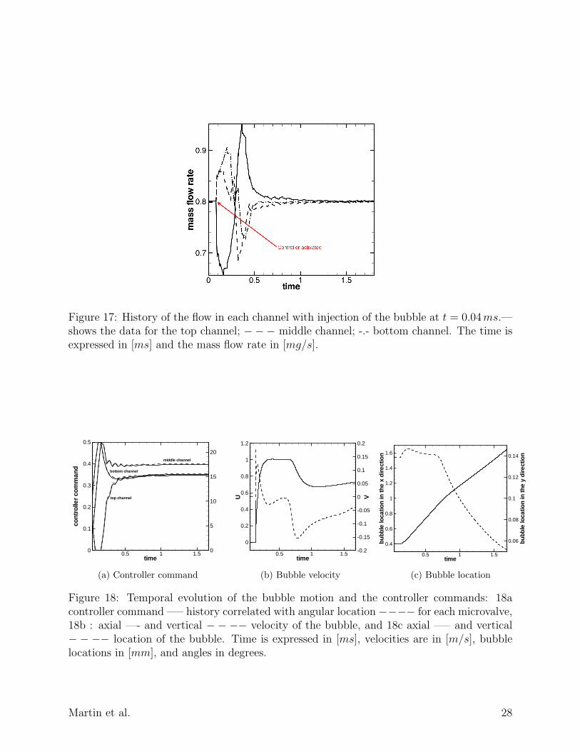
Figure 17: History of the flow in each channel with injection of the bubble at t = 0.04ms.—shows the data for the top channel; −−− middle channel; -.- bottom channel. The time isexpressed in [ms] and the mass flow rate in [mg/s].

time

cont

rolle

rco

mm

and

0.5 1 1.50

0.1

0.2

0.3

0.4

0.5

0

5

10

15

20

top channel

middle channel

bottom channel

(a) Controller command

time

U V

0.5 1 1.5

0

0.2

0.4

0.6

0.8

1

1.2

-0.2

-0.15

-0.1

-0.05

0

0.05

0.1

0.15

0.2

(b) Bubble velocity

time

bu

bble

loca

tion

inth

ex

dire

ctio

n

bu

bble

loca

tion

inth

ey

dire

ctio

n

0.5 1 1.5

0.4

0.6

0.8

1

1.2

1.4

1.6

0.06

0.08

0.1

0.12

0.14

(c) Bubble location

Figure 18: Temporal evolution of the bubble motion and the controller commands: 18acontroller command —– history correlated with angular location −−−− for each microvalve,18b : axial —- and vertical − − −− velocity of the bubble, and 18c axial —– and vertical− − −− location of the bubble. Time is expressed in [ms], velocities are in [m/s], bubblelocations in [mm], and angles in degrees.

Martin et al. 28

7.4.2 Multiple bubble simulation

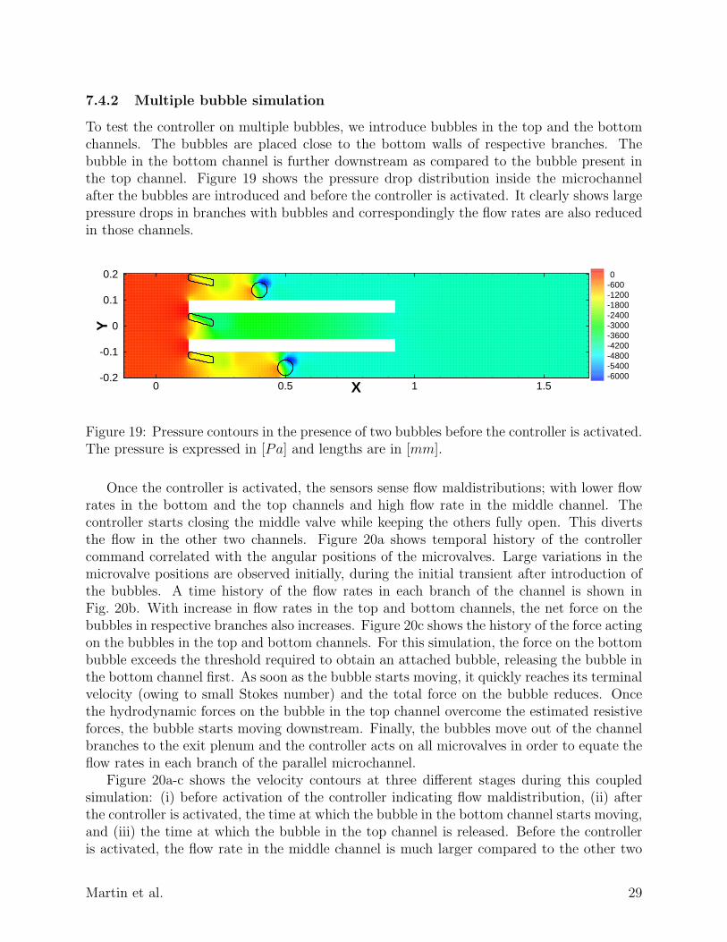
To test the controller on multiple bubbles, we introduce bubbles in the top and the bottomchannels. The bubbles are placed close to the bottom walls of respective branches. Thebubble in the bottom channel is further downstream as compared to the bubble present inthe top channel. Figure 19 shows the pressure drop distribution inside the microchannelafter the bubbles are introduced and before the controller is activated. It clearly shows largepressure drops in branches with bubbles and correspondingly the flow rates are also reducedin those channels.

X

Y

0 0.5 1 1.5-0.2

-0.1

0

0.1

0.2 0-600-1200-1800-2400-3000-3600-4200-4800-5400-6000

Figure 19: Pressure contours in the presence of two bubbles before the controller is activated.The pressure is expressed in [Pa] and lengths are in [mm].

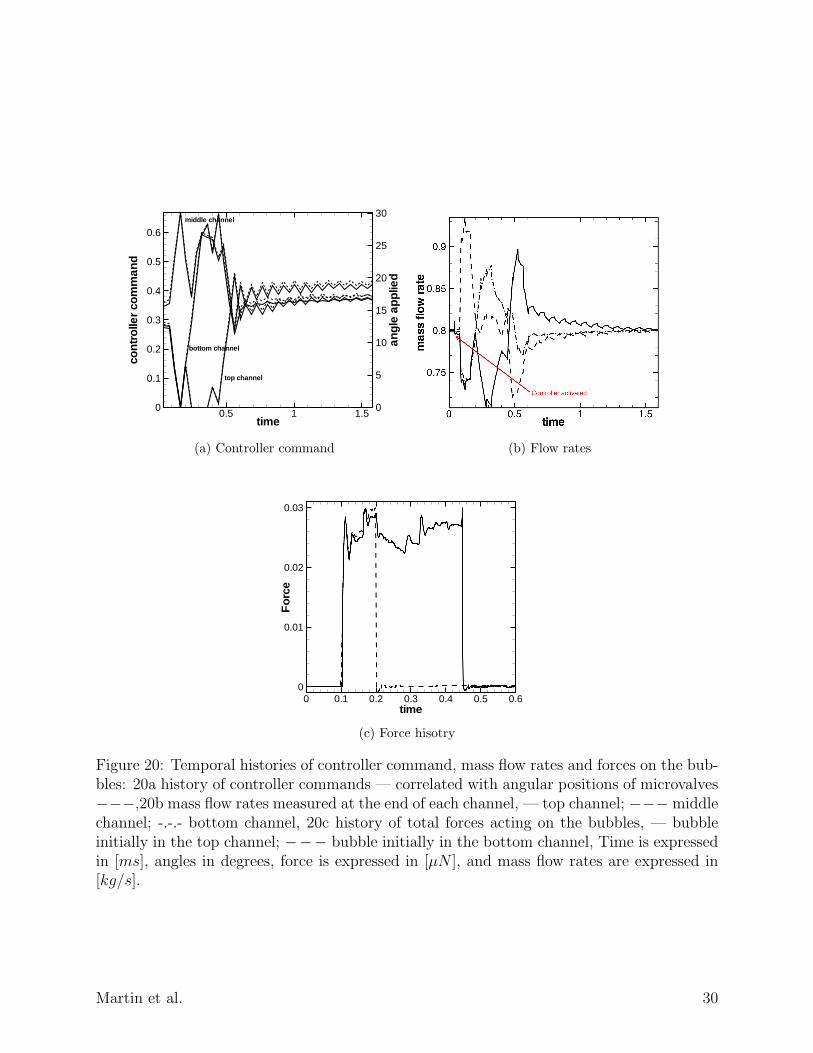
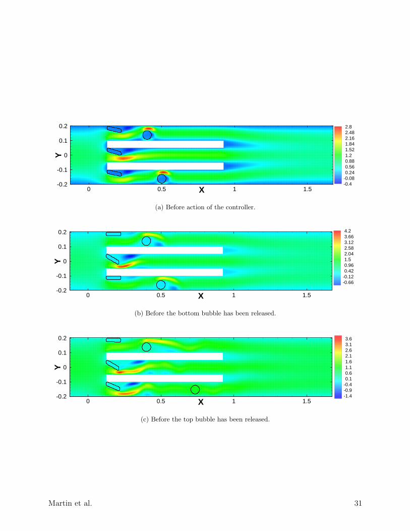
Once the controller is activated, the sensors sense flow maldistributions; with lower flowrates in the bottom and the top channels and high flow rate in the middle channel. Thecontroller starts closing the middle valve while keeping the others fully open. This divertsthe flow in the other two channels. Figure 20a shows temporal history of the controllercommand correlated with the angular positions of the microvalves. Large variations in themicrovalve positions are observed initially, during the initial transient after introduction ofthe bubbles. A time history of the flow rates in each branch of the channel is shown inFig. 20b. With increase in flow rates in the top and bottom channels, the net force on thebubbles in respective branches also increases. Figure 20c shows the history of the force actingon the bubbles in the top and bottom channels. For this simulation, the force on the bottombubble exceeds the threshold required to obtain an attached bubble, releasing the bubble inthe bottom channel first. As soon as the bubble starts moving, it quickly reaches its terminalvelocity (owing to small Stokes number) and the total force on the bubble reduces. Oncethe hydrodynamic forces on the bubble in the top channel overcome the estimated resistiveforces, the bubble starts moving downstream. Finally, the bubbles move out of the channelbranches to the exit plenum and the controller acts on all microvalves in order to equate theflow rates in each branch of the parallel microchannel.

Figure 20a-c shows the velocity contours at three different stages during this coupledsimulation: (i) before activation of the controller indicating flow maldistribution, (ii) afterthe controller is activated, the time at which the bubble in the bottom channel starts moving,and (iii) the time at which the bubble in the top channel is released. Before the controlleris activated, the flow rate in the middle channel is much larger compared to the other two

Martin et al. 29

time

cont

rolle

rco

mm

and

angl

eap

plie

d

0.5 1 1.50

0.1

0.2

0.3

0.4

0.5

0.6

0

5

10

15

20

25

30

top channel

middle channel

bottom channel

(a) Controller command (b) Flow rates

time

For

ce

0 0.1 0.2 0.3 0.4 0.5 0.60

0.01

0.02

0.03

(c) Force hisotry

Figure 20: Temporal histories of controller command, mass flow rates and forces on the bub-bles: 20a history of controller commands — correlated with angular positions of microvalves−−−,20b mass flow rates measured at the end of each channel, — top channel; −−− middlechannel; -.-.- bottom channel, 20c history of total forces acting on the bubbles, — bubbleinitially in the top channel; −−− bubble initially in the bottom channel, Time is expressedin [ms], angles in degrees, force is expressed in [µN ], and mass flow rates are expressed in[kg/s].

Martin et al. 30

X

Y

0 0.5 1 1.5-0.2

-0.1

0

0.1

0.2 2.82.482.161.841.521.20.880.560.24

-0.08-0.4

(a) Before action of the controller.

X

Y

0 0.5 1 1.5-0.2

-0.1

0

0.1

0.2 4.23.663.122.582.041.50.960.42

-0.12-0.66

(b) Before the bottom bubble has been released.

X

Y

0 0.5 1 1.5-0.2

-0.1

0

0.1

0.2 3.63.12.62.11.61.10.60.1

-0.4-0.9-1.4

(c) Before the top bubble has been released.

Martin et al. 31

X

Y

0.5 1 1.5-0.2

-0.1

0

0.1

0.2

(d) Bubble trajectories

Figure 20: Temporal evolution of velocity contours and bubble trajectories in the coupledCFD-cotroller simulation for two bubbles.The lengths are expressed in [mm], the velocity in[m/s].

branches. Once the controller is activated, it closes the microvalve for the middle channel andfully opens the valves in the top and bottom channels. The bubbles are then set in motionand finally escape into the exit plenum, reducing the flow maldistribution. Figure 20d showsthe trajectory of each bubble inside the parallel configuration.

8 Conclusion

We investigated flow maldistribution occurring in parallel microchannels due to presenceof vapor bubbles in certain branches of the channel. In the present work, the bubbly flowregime consisting of small bubbles inside the microchannels was simulated at low Reynoldsnumbers. Neglecting any deformation of the vapor bubble, the bubbles were treated as rigidparticles of density lower than the surrounding fluid. This assumption is reasonable for lowWeber and Reynolds numbers. A novel fictitious-domain based direct numerical simulationapproach was developed to simulate, from first principles, motion of freely moving rigid ob-jects with large density ratios between the object and the surrounding fluid. The approachis also applicable to model flow around rigid microvalves with specified rotational motion.The numerical approach was thoroughly validated over a range of standard numerical testsfor freely moving and specified motion of particles to show good agreements with availableexperimental data. The parallel numerical solver was integrated with a MATLAB-basedmodel-predictive control algorithm to perform coupled CFD-controller simulations whereinthe flow rates in different branches of the microchannels are controlled by activating mi-crovalves at the entrance to the channels.

The goal of these coupled simulations was to first detect flow maldistribution in thepresence of bubbles, and then eliminate any disparity in the flow rates through microvalveactuation. Accordingly, the flow rates in each branch of the microchannel were used as sensorinput. System identification techniques were first employed on numerical simulations of fluidflow through the parallel microchannel in the absence of any bubbles. These studies produceda lower dimensional model that captures the essential dynamics of the full nonlinear flow, in

Martin et al. 32

terms of a relationship between valve angles and the exit flow rate for each channel. A modelpredictive controller was then developed by utilizing this reduced order model to identifyflow maldistribution from exit flow velocities and prescribe actuation of channel valves toeffectively redistribute the flow. Coupled simulations were first applied to single-phase flowin three-channel geometry that equates the flow rates in each branch of the channel. Theapproach was then applied to two-phase flow, with artificially introduced bubbles in certainbranches. The model predictive control methodology was shown to adequately reduce flowmaldistribution by quickly varying channel valves to remove bubbles and equalize flow ratesin each channel. The approach developed is general in the sense that it is also applicableto fouling and clogging of microchannels to presence of rigid particulates. The numericalmodel is efficient and simulations involving particle clusters are feasible due to its parallelimplementation.

Acknowledgment

This work was supported under the US Army’s Tactical Energy Systems program at Ft.Belvoir. The funding was received through the Oregon Nano and Microtechnology Institute(ONAMI) at Oregon State University. All simulations were conducted at the in-house highperformance computing cluster. SVA also acknowledges Dr. Ki-Han Kim of the Office ofNaval Research for the support provided under the ONR grant number N000140610697. Thisresulted in successful implementation of the DNS algorithm for freely moving particles.

Martin et al. 33

9 Appendix

9.1 Interphase Interpolations

Any property defined at the material volumes within the particle can be projected onto thebackground grid by using interpolation functions. Use of simple linear interpolations maygive rise to unphysical values within the particle domain (e.g. volume fractions greater thanunity) [14] and may give rise to numerical oscillations in the particle velocity. In order toovercome this, a smooth approximation of the quantity can be constructed from the materialvolumes using interpolation kernels typically used in particle methods [31]:

Φ∆(x) =

∫Φ(y)ξ∆(x− y)dy (28)

where ∆ denotes grid resolution. The interpolation operator can be discretized using thematerial volume centroids as the quadrature points to give

Φ∆(x) =N∑

M=1

VMΦ(XM)ξ∆(x−XM) (29)

where XM and VM denote the coordinates and volume of the material volumes respectivelyand the summation is over all material volumes for a particle. For example, in order tocompute particle volume fraction, Φ(XM) will be unity at all material points. This givesunity volume fraction within the particle domain and zero outside the particle. In order toconserve the total volume of the particle as well as the total force/torque exerted by theparticle on the fluid, the interpolation kernel should at least satisfy

N∑M=1

VMξ∆(x−XM) = 1 (30)

N∑M=1

VM(x−XM)ξ∆(x−XM) = 0 (31)

Several kernels with second-order accuracy include Gaussian, quartic splines etc. A kernelwith compact support requiring only the immediate neighbors of a control volume has beendesigned and used in immersed boundary methods [17]. For uniform meshes with resolution∆ it utilizes only three points in one dimension and gives the sharpest representation of theparticle onto the background mesh:

ξ∆(x−XM) =1

∆3δ

(x−XM

∆

)δ

(y − YM

∆

)δ

(z − ZM

∆

), (32)

where

δ(r) =

16(5− 3|r| −

√−3(1− |r|)2 + 1, 0.5 ≤ |r| ≤ 1.5, r = (x−x0)

∆13(1 +

√−3r2 + 1, |r| ≤ 0.5

0, otherwise.

(33)

Martin et al. 34

The same interpolation kernel can be used to interpolate an Eulerian quantity defined atthe grid centroids to the material volume centroids. The interpolation kernel is second orderaccurate for smoothly varying fields [32]. The effect of these interpolations is that the surfaceof the particle is smoothed over the scale proportional to the kernel length. Note that inorder to reduce the spreading of the interfacial region, it is necessary to use compact supportas well as finer background grids and material volumes.

9.2 Updating the Particle Position

The rigid body motion (RBM) of a particle can be decomposed into translational (UT ) androtational (UR) components. The total velocity field at each point within the particle isgiven as

URBM = UT + Ω× r (34)

where UT is the translational velocity, Ω the angular velocity, and r the position vector ofthe material volume centroid with respect to the particle centroid. All the material volumeshave the same translational velocity as the particle centroid (UT = UP ).

Given a velocity field and the positions (X0M) of the material volume centroids and the

particle centroid (XP ) at t = t0, the new positions (XtM) at t = t0 + ∆t are obtained by

linear superposition of the rotational and translational components of the velocity. The axisof rotation passing through the rigid body centroid XP is given as σ = Ω/ |Ω|. The newcoordinates due to rotation around σ are given as

X′ = R(X0M −XP ) + XP (35)

where the rotation matrix is

R =

tσxσx + c tσxσy − sσz tσxσz + sσytσxσy + sσz tσyσy + c tσyσz − sσxtσxσz − sσy tσyσz + sσx tσzσz + c

. (36)

Here c = cos(α), s = sin(α), t = 1− cos(α), and α = |Ω|dt. The material volume centroidsare all uniformly translated to give the final positions,

XtM = X′ + UTdt. (37)

Martin et al. 35

References

[1] Qu, W. and Mudawar, I., 2003, “Flow boiling heat transfer in two-phase micro-channelheat sinks—-i. experimental investigation and assessment of correlation methods,” In-ternational Journal of Heat and Mass Transfer, 46(15), pp. 2755–2771.

[2] Triplett, K., Ghiaasiaan, S., Abdel-Khalik, S., and Sadowski, D., 1999, “Gas–liquidtwo-phase flow in microchannels part i: two-phase flow patterns,” International Journalof Multiphase Flow, 25(3), pp. 377–394.

[3] Cubaud, T., 2004, “Transport of bubbles in square microchannels,” Physics of Fluids,16(12), p. 4575.

[4] Sharp, K. and Adrian, R., 2005, “On flow-blocking particle structures in microtubes,”Microfluidics and Nanofluidics, 1(4), pp. 376–380.

[5] Wang, E., Shankar, D., Hidroo, D., CH Fogg, Koo, J., Santiago, J., Goodson, K., andKenny, T., 2004, “Liquid velocity field measurements in two-phase microchannel convec-tion,” 3rd International symposium on Two-phase Flow Modeling and Experimentation.

[6] Lee, P., Tseng, F., and Pan, C., 2004, “Bubble dynamics in microchannels. part i: singlemicrochannel,” International Journal of Heat and Mass Transfer, 47(25), pp. 5575–5589.

[7] Li, H., Tseng, F., and Pan, C., 2004, “Bubble dynamics in microchannels. part ii: twoparallel microchannels,” International Journal of Heat and Mass Transfer, 47(25), pp.5591–5601.

[8] Mukherjee, A. and Kandlikar, S., 2005, “Numerical study of the effect of inlet con-striction on bubble growth during flow boiling in microchannels,” 3rd InternationalConference on Microchannels and Minichannels, ICMM2005, vol. 75143.

[9] Bleris, L., Garcia, J., Arnold, M., and Kothare, M., 2006, “Model predictive hydro-dynamic regulation of microflows,” Journal of micromechanics and microengineering,16(9), p. 1792.

[10] Glowinski, R., Pan, T., Hesla, T., Joseph, D., and Periaux, J., 2001, “A fictitiousdomain approach to the direct numerical simulation of incompressible viscous flow pastmoving rigid bodies- application to particulate flow,” Journal of Computational Physics,169(2), pp. 363–426.

[11] Patankar, N., 2001, “A formulation for fast computations of rigid particulate flows,”Center for Turbulence Research Annual Research Briefs 2001, pp. 185–196.

[12] Apte, S. V., Martin, M., and Patankar, N., 2008, “A numerical method for fully re-solved simulation (frs) of rigid particle-flow interactions in complex flows,” Journal ofComputational Physics.

[13] Patankar, N., Singh, P., Joseph, D., Glowinski, R., and Pan, T., 2000, “A new formu-lation of the distributed Lagrange multiplier/fictitious domain method for particulateflows,” International Journal of Multiphase Flow, 26(9), pp. 1509–1524.

Martin et al. 36

[14] Sharma, N. and Patankar, N., 2005, “A fast computation technique for the direct numer-ical simulation of rigid particulate flows,” Journal of Computational Physics, 205(2),pp. 439–457.

[15] Kim, D. and Choi, H., 2000, “A second-order time-accurate finite volume method forunsteady incompressible flow on hybrid unstructured grids,” Journal of ComputationalPhysics, 162(2), pp. 411–428.

[16] Mahesh, K., Constantinescu, G., Apte, S., Iaccarino, G., Ham, F., and Moin, P., 2006,“Large-Eddy Simulation of Reacting Turbulent Flows in Complex Geometries,” Journalof Applied Mechanics, 73, p. 374.

[17] Roma, A., Peskin, C., and Berger, M., 1999, “An Adaptive Version of the ImmersedBoundary Method,” Journal of Computational Physics, 153(2), pp. 509–534.

[18] Ferziger, J. and Peric, M., 2002, Computational methods for fluid dynamics, SpringerNew York.

[19] van der Vorst, H., 2003, Iterative Krylov Methods for Large Linear Systems, CambridgeUniversity Press.

[20] Ham, F. and Young, Y., 2003, “A Cartesian Adaptive Level Set Method for Two-PhaseFlows.” Annu. Research Briefs, 2003: Center for Turbulence Research.

[21] Leung, L., 1999, System Identification - Theory for the user, Prentice Hall.

[22] Zhu, Y., 2001, Multivariable System Identification for Process Control, Elsevier Science.

[23] Camacho, E. and Bordons, C., 2004, Model Predictive Control, Springer-Verlag.

[24] Qu, W., Mudawar, I., Lee, S., and Wereley, S., 2006, “Experimental and computationalinvestigation of flow development and pressure drop in a rectangular micro-channel,”Journal of Electronic Packaging, 128, p. 1.

[25] Dutsch, H., Durst, F., Becker, S., and Lienhart, H., 1998, “Low-reynolds-number flowaround an oscillating circular cylinder at low keulegan–carpenter numbers,” Journal ofFluid Mechanics, 360, pp. 249–271.

[26] Lomholt, S., Stenum, B., and Maxey, M., 2002, “Experimental verification of the forcecoupling method for particulate flows,” International Journal of Multiphase Flow, 28(2),pp. 225–246.

[27] Kim, D. and Choi, H., 2006, “Immersed boundary method for flow around an arbitrarilymoving body,” Journal of Computational Physics, 212(2), pp. 662–680.

[28] Mordant, N. and Pinton, J., 2000, “Velocity measurement of a settling sphere,” TheEuropean Physical Journal B, 18(2), pp. 343–352.

[29] Finn, J., 2009, “A multiscale modeling approach for bubble-vortex interactions in hydro-propulsion systems,” M.S. Thesis, Oregon State University, Corvallis, OR.

Martin et al. 37

[30] Shridhar, R. and Cooper, D., 1998, “A Tuning Strategy for Unconstrained MultivariableModel Predictive Control,” Industrial and Engineering chemistry research, 37, pp. 4003–4016.

[31] Koumoutsakos, P., 2005, “Multiscale flow simulations using particles,” Annual Reviewof Fluid Mechanics, 37(1), pp. 457–487.

[32] Peskin, C., 2003, “The immersed boundary method,” Acta Numerica, 11, pp. 479–517.

Martin et al. 38