Embed Size (px)
Citation preview

Edith Cowan University Edith Cowan University
Research Online Research Online
Theses : Honours Theses
2002
Direct sequential simulation algorithms in geostatistics Direct sequential simulation algorithms in geostatistics
Robyn Robertson Edith Cowan University
Follow this and additional works at: https://ro.ecu.edu.au/theses_hons
Part of the Geology Commons, and the Statistical Methodology Commons
Recommended Citation Recommended Citation Robertson, R. (2002). Direct sequential simulation algorithms in geostatistics. https://ro.ecu.edu.au/theses_hons/562
This Thesis is posted at Research Online. https://ro.ecu.edu.au/theses_hons/562

Edith Cowan University
Copyright Warning
You may print or download ONE copy of this document for the purpose
of your own research or study.
The University does not authorize you to copy, communicate or
otherwise make available electronically to any other person any
copyright material contained on this site.
You are reminded of the following:
Copyright owners are entitled to take legal action against persons who infringe their copyright.
A reproduction of material that is protected by copyright may be a
copyright infringement. Where the reproduction of such material is
done without attribution of authorship, with false attribution of
authorship or the authorship is treated in a derogatory manner,
this may be a breach of the author’s moral rights contained in Part
IX of the Copyright Act 1968 (Cth).
Courts have the power to impose a wide range of civil and criminal
sanctions for infringement of copyright, infringement of moral
rights and other offences under the Copyright Act 1968 (Cth).
Higher penalties may apply, and higher damages may be awarded,
for offences and infringements involving the conversion of material
into digital or electronic form.

Direct Sequential Simulation Algorithms
in Geostatistics
A Thesis Submitted to the
Faculty of Communications, Health and Science
Edith Cowan University
Perth, Western Australia
by Robyn Robertson
In Partial Fulfillment of the Reqm:rements for the Degree
of
Bachelor of Science Honours (Mathematics)
December 2002
Supervisors: Dr Ute Mueller
Associate Professor Lyn Bloom

USE OF THESIS
The Use of Thesis statement is not included in this version of the thesis.

Abstract
Conditional sequential simulation algorithms have been used in geostatistics for many
years but we currently find new developments are being made in this field. This thesis
presents two new direct sequential simulation with histogram reproduction algorithms
and compares them with the efficient and widely used sequential Gaussian simulation
algorithm and the otiginal direct sequential simulation algorithm. We explore the
possibility of reproducing both the semivariogram and the histogram without the need
for a transformation to nmmal space, through optimising an objective function and
placing linear constr·.tints on the local conditional distributions. Programs from the
GSLIB Fortran library are expanded to provide a simulation environment. An isotropic
and an anisotropic data set are analysed. Both sets are positively skewed and the
exhaustive data is available to define global target distributions and for comparing the
cumulative distribution functions of the simulated values.

To
Nathan, Kaylee, Stephen & Louise.
II

I Declaration I
I certify that this thesis does not, to the best of my knowledge and belief
(i) incorporate without acknowledgement any material previously submitted for
a degree or diploma in any institution of higher education;
(ii) contain any material previously published or written by another person
except where due reference· is made in the text; or
(iii) contain any defamatory material.
Signature:
Date: .~~)2.Jo.3 ................... ..
Ill

Acknowledgements
I wish to express my deepest thanks to my children Nathan, Kaylee, Stephen and Louise
for their love, support and patience which has enabled me to complete my degree. I also
wish to thank my supervisors Ute Mueller and Lyn Bloom for their help and guidance in
completing my degree and thesis at Edith Cowan University.
iv

Table of Contents
Abstract ..................................................................................................................... .i
Dedication ................................................................................................................ .ii
Declaration .............................................................................................................. iii
Acknowledgements ................................................................................................. .iv
1 Introduction ............................................................................................ l
1.1 Background and Significance ........................................................................ !
1.2 Objective of the Study .................................................................................... 3
1.3 Thesis Outline ................................................................................................. 3
1.4 Notation .......................................................................................................... 4
2 Geostatistical Framework ..................................................................... 6
2.1 Random Functions .......................................................................................... 6
2.2 Distributions ................................................................................................... 7
2.3 Stationarity ...................................................................................................... 7
2.4 Relationship between Covariogram and Semivariogram ............................... 9
2.5 Inference and Modelling ............................................................................... 10
2.6 Range and Si11. .............................................................................................. 10
2.7 The Nugget Effect ........................................................................................ 11
2.8 Isotropy and Anisotropy ............................................................................... 12 . . -·· .. . ...... - -v

2.8.1 Geometric Anisotmpy ............................................................... 12
2.8.2 Zonal Anisotropy ...................................................................... 12
2.9 Isotropic Semivariogram Models .............................................................. 13
2.9.1 Nugget effect model. ................................................................. 13
2.9.2 Spherical model ........................................................................ 14
2.9.3 Exponential model .................................................................... 14
2.9.4 Gaussian model. ........................................................................ 15
2.9.5 Power model ............................................................................. 15
2.10 Kriging ..................................................................................................... 15
2.10.1 Simple Kriging ......................................................................... 16
2.11 Simulation ................................................................................................ 17
3 Sequential Simulation Methods and their lmplementation ....•....•.• 19
3.1 Sequential Simulation Algorithm .............................................................. 19
3.2 Parametric Algorithms .............................................................................. 20
3.2.1 Sequential Gaussian Simulation ................................................ 20
3 .2.2 Direct Sequential Simulation ..................................................... 21
3.3 Non-Parametric Algorithms ...................................................................... 21
3.3 .1 Direct Sequential Simulation with Histogram Identification ...... 21
3.4 Constrained Optimisation .......................................................................... 24
3.5 Linear Programming Problems .................................................................. 24
3.6 One-norm Approximation with Linear Constraints .................................... 28
3.7 Quadratic Programming ............................................................................ 29
3.8 Implementation and Specifications ............................................................ 31
3.8.1 Sequential Gaussian simulation- SGSIM .................................. 33
vi

3.8.2 Direct sequential simulation ........................................................ 33
3.8.3 DSSIM- Original direct sequential simulation ........................... 33
3.8.4 Direct sequential simulation with histogram reproduction .......... 34
3.8.5 DSSL1 -Direct sequential simulation with histogram ................ 34 reproduction using the one-norm
3.8.6 DSSL2- Direct sequential simulation with histogram ............... 37 reproduction using the two-norm
4 Performance Assessment ••••••..••...••••••••..•.••••••.•••...•...•••••••••......•••••••••.. 39
4.1 Qualitative Assessment ................................................................................ 39
4.1.1 Probability Maps .......................................................................... 39
4.1.2 Quantile Maps .............................................................................. 39
4.1.3 Conditional Vnriance ................................................................... 40
4.2 Quantitative Assessment .............................................................................. 40
4.2.1 Histogram Reproduction .............................................................. 41
4.2.2 Semivariogram Reproduction ...................................................... 42
5 Application to the Isotropic Case ....................................................... 43
5.1 Exploratory Data Analysis ........................................................................... 43
5.2 Vnriography .................................................................................................. 45
5.3 Simu1ation ..................................................................................................... 48
5.4 Histogram Reproduction .............................................................................. 51
5.5 Vnriograrn Reproduction .............................................................................. 60
5.6 Spatial Uncertainty ....................................................................................... 62
vii

5.7 Summary for Penneability ........................................................................ 65
6 Application to the Anisotropic Case ................................................. 66
6.1 Exploratory Data Analysis ........................................................................ 66
6.2 Variography .............................................................................................. 68
6.3 Simulation ................................................................................................ 71
6.4 Histogram Reproduction ........................................................................... 72
6.5 VariogramReproduction ........................................................................... 82
6.6 Spatial Uncertainty ................................................................................... 84
6. 7 Summary for Potassium ............................................................................ 89
7 Results and Conclusions ................................................................... 90
8 References .......................................................................................... 94
9 Appendices ......................................................................................... 96
9.1 Appendix A .............................................................................................. 96
9.2 Appendix 8. ............................................................................................ j02
viii

1 Introduction
1.1 Background and Significance
Geostatistics developed from a need to evaluate recoverable reserves in mineral de
posits and provides statistical tools for the description and modelling of spatial and
spatiotemporal variables. It takes into account both the structure and the random
ness inherent in any deposit. In 1962 G. Matheron defined geostatistics as "the
application of the formalism of random functions to the reconnaissance and estima
tion of natural phenomena.'' Geostatistics can be considered as a set of statistical
procedures that deal with the characterisation of spatial attributes. Geostatistics
is now used in many different fields, wherever there is a need for evaluating spa
tially correlated data, such as in mining, petroleum, oceanography, hydrogeology
and environmental science.
The two principal components of geostatistics are estimation and simulation. Es
timation is used to infer attribute values at unsampled locations from the (known)
values at sampled locations. The most common geostatistical estimation method is
lcriging, which is a generalised linear regression technique that provides at each lo
cation a best linear unbiased estimator (BLUE) for the unknown attribute studied.
Many variants of kriging have been developed, but all rely on the same concepts.
Three types of parametric kriging for a single attribute can be differentiated de
pending on the model used for the mean (Remy et al, 2001). These are termed
simple kriging (SK), ordinary kriging (OK) and kriging with a trend model (KT).
A non-parametric type of kriging is indicator kriging (IK).
Least-squares interpolation algorithms tend to smooth out local details of the
spatial variation of the attribute (Goovaerts, 1998). Kriging tends to unevenly
smooth the data, that is, kriging estimates have less spatial variability than the
real values and the smoothing is inversely proportional to the data density. Con
sequently values below the sample mean are overestimated and values above the
sample mean are underestimated. The smoothing distortion is also evidenced by
the experimental semivariogram of the estimates differing from the sampling experi
mental semivariogram, and the histogram of the sample differing from the histogram
1

of the estimated values (Olea, 1999).
Conditional simulation was initislly developed to correct the smoothing effect
produced by kriging (Deutsch & Journel, 1998). Conditional simulations are spa
tially consistent Monte Carlo simulations (Chiles and Delfiner, 1999) and are used
to characterise the uncertainty associated with the prediction of attril'mte values at
unsampled location..c; while honouring the data values at sample locations. A large
number of equiprobable realisations are generated so as to obtain global accuracy
by the reproduction of properties such as histograms and semivariograms. Condi
tional simulations are used qualitatively to obtain maps of spatial variability, and
quantitatively to evaluate the effect of spatial uncertainty on the results of complex
procedures, allowing for sensitivity and risk analysis.
Sequential simulation is a widely accepted and computationally efficient tool used
to obtain simulations that reproduce df'.sired properties through the use of condi
tional distributions. Sequential Gaussian simulation is one of the main methods that
rely on the multi Gaussian approach. At each unsampled location, an observation is
randomly drawn from the normal distribution with mean equal to the simple kriging
mean and variance equal to the simple kriging variance. Journel {1994) showed that
this normality assumption can be relaxed, and any type of local conditional distrib
ution can be used to simulate the values, as long as its mean and variance are equal
to the simple kriging parameters. This led to the development of direct sequential
simulation (dss), which ensures variograrn reproduction but not necessarily global
histogram reproduction.
In this study we explore two direct sequential simulation algorithms with his
togram reproduction, the first using the one norm ( dssPl) and the second the two
norm {dss£2). We examine the possibility of a simulation algorithm being able tore
produce both the histogram and the experimental semivariogram model without the
need for a transformation to normal space. This project allows us to link numer
ical analysis, operations research and computer programming with geostatistics.
Fortran code was developed by modifying and adding to GSLIB code, and other
programs were incorporated with this to achieve the programs required to run the
simulation algorithms.
2

1.2 Objective of the Study
In this study we develop and investigate in detail, a new direct sequential simulation
technique dssl2 and compare it to earlier direct sequential simulation methods dss
and dssfl and also to sequential Gaussian simulation. This new direct sequential
simulation algorithm that uses quadratic programming to determine local condi
tional probability distributions from which the resulting realisations will depend on.
In addition, the algorithms for sequential Gaussian simulation and the earlier direct
sequential simulation methods will be outlined and discussed.
These simulation algorithms are applied to sample data sets that have different
statistical and spatial features, and the results are evaluated and compared. Two
data sets, Permeability and Potassium, have been selected for analysis, in order
to present comparisons of the simulation methods. Both data sets are positively
skewed, albeit only slightly for Potassium. The two data sets also exhibit differ
ent patterns of spatial continuity. The Permeability data are isotropic, while the
Potassium data are anisotropic.
1.3 Thesis Outline
Chapter 2 presents the theoretical background of the random function model, sta
tionarity and simple kriging. In Chapter 3 we look at sequential simulation algo
rithms, outline the mathematical background of optimisation and discuss the imple
mentation of the simulation algorithms. In Chapter 4 we discuss the programming
algorithms developed in the research. In Chapter 5 and Chapter 6 the isotropic
data set and the anisotropic data set respectively, are presented. We present the
quantitative and qualitative performance assessments used in this study in Chapter
7. In Chapter 8 we discuss the results and findings of the study.
3

1.4 Notation
The gcostatistical notation used in this thesis follows Goovaerts (1997) and the
GSLIB user's manual (Deutsch & Journel, 1998). In particular:
V for all
A study region
a
G(O)
G(h)
Cov f.l E{-)
F(u;z)
F(u; zi (n))
range parameter
stationary variance of the random variable
Z(u)
stationary covariace of the random function
Z(u) for lag h
covariance
expected value·
cumulative distribution function of the ran-
dom variable Z(u)
conditionat cumulative distribution function
of a random variable Z(u)
F(up ... , UNjZ1, .•• , zN)multivariate cumulative distribution func
tion
,Q(h)
!(h)
t(h) h= lhl h
/(
~~K (u)
m(u)
m
N(h)
model semivariogram at lag vector h
semivariogram at lag vector h
experimental semivariogram at lag vector h
separation distance or Jag
separation vector
number of threshold values Zk
Simple Kriging weight of attribUte value at
sampled location Ua for estimation of the at
tribute value at location u
expected value of the random variable Z(u)
constant mean of the random variable Z(u)
number of sample data pairs separated by lag
vector h
4

n
p(h)
llullt I lull, Var{•)
Z(u)
z(u)
z(u.)
Z(u.)
Z'(u)
number of data values z(ua) available over
the region A
correlogram of the random function Z(u) at
lag vector h
one-norm
two-norm
variance
random variable at sample location u
actual attribute value at location u
sample attribute value at location u
random variable at location. Ua
random variable of estimated value at loca
tion u
Simple Kriging estimator of Z(u)
5

2 Geostatistical Framework
2.1 Random Functions
Geostatistics deals with the characterisation of spatial attributes in a given region
A in two- or three-dimensional space. The attribute values are usually only known
at some locations in the region A and in order to carry out any statistical infer
ence it is necessary to impose a conceptual model that will allow one to obtain a
realisation of the attribute over the entire region. This conceptual model is known
as the random function model. Suppose that the attribute values are known at the
locations ua E A, a = 1, ... , n. A known sample value z(ucr) is considered as one
particular realisation of a random variable Z{uQ'). Any unknown attribute z(u) is
regarded as one realisation of a random variable Z(u) (Armstrong, 1998; Chiles &
Delfiner, 1999; Goovaerts, 1997). The random variable Z(u) is completely defined
by its cumulative distribution function given by
F(u;z) = Pr{Z(u) $z} for all z E JR. (1)
The family of (usually) dependent random variables {Z(u), u E A} is called a
random function. The random function is fully characterised by the set of all its
N-variate cumulative distribution functions, for any number N and any choice of
the N locations Un 1 n = 1, ... , N:
F(u, ... , u";z, ... ,z") = Pr {Z (u,) 9,. .. , Z (u") $zN} (2)
A multivariate cumulative density function is used to model the joint uncertainty
about the N values z(u1), ••• ,z(uN). Generally, the number of data available is
insufficient to infer the joint distribution function, so in practice the spatial analysis
is limited to cumulative density functions involving no more than two locations at a
time, and their corresponding moments. The first two moments of the distribution
provide an w::ceptable approximate solution.
6

2.2 Distributions
Most of the theoretical concepts in geostatistics rely on data that follow a particular
probability distribution. The most widely used of these is the Gaussian or 'nor
mal' distribution whose probability density function, called the normal curve, is the
symmetric bell-shaped curve with positive and negative tails that stretch to infin
ity in both directions. The probability density function of the normal probability
distribution (Walpole & Myers, 1989) with mean Jl and variance u2, is given by
1 (1 (z-~)') g(z) = av'2ii' exp 2 -a- ' where - oo < z < oo. (3)
The standard normal distribution has mean Jl = 0 and variance u2 = 1, and in this
case Equation (3) becomes
g(z) =- exp --1 ( z') y'2ii' 2
where - oo < z < oo. (4)
Any normal random variable Z with mean J.t and standard deviation acan be trans
formed to a standard normal random variable Y by letting
z-~ Y=--. a
Another distribution often used in geostatistics is the lognormal distribution,
where the logarithms of the data values are normally distributed. The lognormal
model is a natural choice for positively skewed data such as gold grades, pollution
levels and permeability. The random variable Z is lognormal if Y = log Z is normal.
A logarithmic transformation can convert a skewed variable into a more symmetric
form, and it may also be useful in stabilising the variance. When the variance is
proportional to the mean, a logarithmic transformation may be able to correct this
condition.
2.3 Stationarity
In the case of the data under consideration in geostatistics, repeated measurements
at any one location are usually impossible so a structure needs to be imposed on
7

the random function that enables us to carry out statistical inference. The ob
served data z(Ua), a= 1, · · ·, n are considered as a single realisation of the process
{Z(u): u EA}. When replication of data is not available, this can be overcome
with assumptions concerning the spatial behaviour. A random function is said to be
stationary if the probabilistic structure looks similar in different parts of the study
region A. Replication within a single set of data is then possible from different
subregions.
A random function is stationary within a study region A if its multivariate
cumulative density function is invariant under translation, that is, the characteristics
of a random function stay the same when shifting a given set of N points from
one part of the study region to another. A random function is said to be strictly
stationary if for any set of N locations u1 , ••• , uN and any translation vector h
F(u1 , ••• , uN;z11 ... ,zN) = F(u1 + h, ... , uN + h;z11 ••• ,zN) (5)
As long as two pairs of observations have the same separation vector h, they both
can contribute in the estimation of z(u). The vector h is called the lag vector
between two spatial locations.
A random function is said to be second-order stationary when the mean E{Z(u)}
exists and does not depend on the location u, and the covariance function C (h) exists
and depends only on the separation vector h:
E(Z(u)} = E{Z(u+h)}
Cov{Z(u),Z(u +h)}= C(h)
C (0) = Var{Z(u)}
(6)
(7)
(8)
Second-order stationarity assumes the existence of a finite variance. There are
many physical phenomena, for example Brownian Motion (Serway & Beichner,
2000), and associated random functions that do not have a finite variance or covari
ance, so the assumption of strict stationarity is replaced by the weaker hypothesis
of second-order intrinsic stationarity. An intrinsic random function assumes that
for every vector h the increment Z (u +h) - Z (u) is second-order stationary and
is characterised by the relationships
E{Z(u+h)- Z(u)} = 0 (9)
8

and
Var{Z(u+h)- Z(u)} = 27(h) (10)
where 2f(h) is the variogram function. The semivariogram -y(h) shows how the
dissimilarity between Z (u) and Z (u +h) changes with separation h. The greater
the value of 1{h), the less close the relationship between values at points separated
by h. The semivariogram is an even, nonnegative function equal to 0 at h = 0:
7(h) =7(-h) 7(h) ~ 0 7(0) =D (11)
The parameters commonly used to summarise the bivariate behaviour of a sta
tionary random function are the covariance function C (h), correlogram p {h), and
semivariogram 7 (h) and these are related by:
1 (h) = C (D) - C(h) (12)
(h)= C(h) = 1- 7(h) P C (D) C(D)
(13)
The correlogram expresses how the correlation between locations changes with spa
tial separation.
If a random process is second-order stationary, then it is also intinsically station
ary, but the converse is not true. That is, if C{h) is defined, then the semivariogram
is necessarily defined, but the existence of the semivariogram does not imply the
existence of C(h). If the process is intrinsically stationary but not second-order
stationary, the covariance function does not exist. This is evident in the power var
iog::arn 7(h) = blhiP with 0 < p < 2 and b > 0, which cannot be obtained from a
covariance function as it is unbounded.
2.4 Relationship Between Covariogram and Semivariogram
Assuming that the process is second-order stationary so that C(O) is defined, then
C(D) = Var{Z(u)}. A second order stationary process has C(h) ~ 0, from which
IC(h)l ::> C(O) and C(D) ~ 0. AB llhll increases C(h) tends to zero, so the semivar
iogram of a second-order stationary process has an asymptote equal to 0{0). This
helps to provide a way of checking for stationarity. The semivariogram of the process
9

should flatten out with increasing separation distance of data points. If the semi
variogram steadily increases then the process is not second-order stationary. The
semivariograru is intrinsically stationary if
21(h) --> o as IJhll --+ oo llhll'
2.5 Inference and Modelling
(14)
Once a random function model is chosen, its parameters, the mean and covariance,
are inferred from the sample information available over the study region A. The
sample statistics are used as estimates of population parameters, so the sample needs
to be representative of the study region.
The semivariogram, rather than the covariance, is commonly used to model
spatial variability, although kriging systems are more easily solved with covariance
matrices (Deutsch & Journel, 1998). The semivariogram measures the average dis
similarity between data separated by a vector h and is inferred by the sample (ex
perimental) semivariogram, whereas the covariance measures similarity. The sample
semivariogram used for modelling is computed as half the average squared difference
between the attribute values of every data pair:
1 N(h)
'i (h) = 2N(h) !; [z(u.) - z(u, + h)]2 (15)
where z(ua) and z(ua+h) are the data values at locations Ua and ua+h respectively,
and N(h) is the number of pairs of data values separated by the vector h. The sample
semivariogram may not tend to zero when h tends to zero, although by definition
/(0) = 0.
2.6 Range and Sill
The rate of increase of the sample semivariograrn with distance indicates how quickly
the influence of a sample reduces with distance. The sample semivariogram can
increase indefinitely if the variability of the attribute has no limit at large distances,
10

and this is indicative of nonstationary behaviour. If the random function is second
order stationary, the sample sernivariogram fluctuates about a limiting value, and the
range of the spatial process is the distance at which this limit is reached. This limit
is called the sill of the semivariogram and it signifies that after a certain separation
distance there is no longer any correlation between samples. (Armstrong, 1998}. If
the semivariogram approaches its sill asymptotically, then the practical range is the
value at which the semivariogram reaches 95 % of its sill. The variograrn can reveal
nested structures, each characterised by its own range (Chiles & Delfiner, 1999}.
The sample semivariogram provides a set of experimental values for a finite
number of lags, hkl k = 1, ... ,K, and directions. Continuous functions must be
fitted to these experimental values so as to deduce semivariogram or covariance
values for any possible lag h required b:v kriging, and also to smooth out sample
fluctuations. (Goovaerts, 1997}.
2. 7 The Nugget Effect
From the definition of the semivariogram we have:
7(h) = 7( -h) and 1(0) = 0 (16)
In some applications "t(h) tends to eo i 0 as h tends to 0. This implies that
observation differences at the same location have a positive variance. This is due to
measurement error and/or a spatial process operating at lag distances shorter than
the smallest lag observed in the data set. If this micro-scale process has sill CMs and
if aLE denotes the variance of the measurement error, then
- 2 + Co - (J ME CMS• (17)
'When either of the two components is not zero, the semivariograrn exhibits a discon
tinuity at the origin. This discontinuity at the origin is called the nugget effect. The
term originated from the idea that gold nuggets are dispersed thoughout a larger
body of rock but (possibly) at distances smaller than the smallest sampling distance.
When a sendvariogram has nugget eo and sill C (0), the difference C (0) - C{) is called
11

the partial sill of the semivariogram. The nugget effect is obvious in many data sets.
In the absence of measurement error, the nugget effect is an indication that the
sampling interval was not small enough.
2.8 Isotropy and Anisotropy
The covariance and the semivariogram are said to be anisotropic if they depend
on both distance and direction. They are said to be isotropic if they depend only
on the magnitude of h. When experimental semivariograms exhibit anisotropy, a
coordinate transformation can be applied to obtain an isotropic model. ( Goovaerts,
1997; Wackernagel, 1998). To determine the presence of anisotropy we need to
look at directional experimental semivariograms. A semivariogram surface, which
is essentially a contour plot of the directional semivariograrns, visually indicates
the direction of greatest spatial continuity. It is important that any pronounced
anisotropy is modelled and not ignored. Anisotropy can be classified as either gecr
metric anisotropy or zonal anisotropy.
2.8.1 Geometric Anisotropy
A semivariogram has a gr..:ometric anisotropy when it has the same sill in all direc
tions but different ranges in at least two directions. A plot of the calculated range
of the semivariogram in various directions appears ellipsoidal, and this ellipse can
be transformed to a circle with radius equal to the minor axis via a rotation and
subsequent dilation.
2.8.2 Zonal Anisotropy
A semivariograrn exhibits zonal anisotropy when its sill values vary with direction.
This type of anisotropy can be modelled as the sum of two components; an isotropic
semivariogram in both coordinates and a one-dimensional semivariogram that de
pends only on the distance in the direction of greater variance. The coordinate
12

system is rotated so that the y-rods coincides with the direction of maximum conti
nuity.
Thus a semivariogram model is completely specified by stating the direction of
greatest continuity, and the anisotropy ratio {minor/major axis in the case of geo
metric anisotropy, and zero in the case of zonal anisotropy) and a suitable isotropic
model function In the next section we will consider isotropic semivariogram models.
These basic models are used to form a linear model that can be isotropic or display
either type of anisotropy.
2.9 Isotropic Semivariogram Models
Only certain functions can be used as models for semivariograms and covariances.
Covariances must be positive definite functions, and so semivariograms have to be
conditionally negative semi-definite, that is
n n
L;L;a;a;2'Y(u, -u;) :S 0 (18) i=l j=l
for any set of locations uP ... , 11n and constants aP ... , an. It is common practice
to fit a positive linear combination of basic models that are known to be permis
sible (Goovaerts, 1997). This eliminates the need to test the permissibility of a
semivariogram model after it has been constructa:l.. The following isotropic semi
variogram models depend only on scalar differences between the locations, h = I hi, not directions.
2.9.1 Nugget effect model
The nugget effect model is a semivariogram for a pure white-noise process. It is
defined by
9 (h) = J 0 for h = 0
l c forh>O (19)
where c;::: 0. The nugget effect is used to model a discontinuity at the origin of the
semivariogram and since it reaches the sill as soon as h > 0, it is bounded.
13

2.9.2 Spherical model
The spherical model has range a and sill c. It is defined by
- { (3h I (h)') 9 (h) = : 2;;- 2 ;;
for0$h<a {20)
for h 2:: a
where Cs 2:: 0. The semivariogram exhibits linear behaviour near the origin, and once
the range is reached, the semivariogram is bounded and remains constant.
2.9.3 Exponential model
The exponential model reaches its sill asymptotically and has a practical range a.
The model is defined by
{21)
The exponential model is bounded and exhibits linear behaviour near the origin.
Differentiating the spherical and exponential model functions with respect to h,
we find the gradient of the spherical model at the origin is
rJ (0) = ( 3 3h')l 2a 2a3 h=o
3 2a
and the gradient of the exponential model is
g' (0) = ~exp (-3h) I a a h=O
3 a
{22)
{23)
Clearly we have ;a <~for all values of a E JR., so the exponential model is steeper
near the origin.
14

2.9.4 Gaussian model
The Gaussian model has practical range a and is bounded as it reaches the sill c
asymptotically. It is defined by
g(h) = c(l-exp (-3:,')) for h 2:0 (24)
The model exhibits parabolic behaviour near the origin, and is infinitely differen
tiable everywhere. It is characteristic of highly regular attributes.
2. 9.5 Power model
The power model is unbounded and has no sill. It is defined by
g(h) = ch" for h 2:0 (25)
where 0 < w < 2, w E lit The power model plays an important role in the theory of
turbulence and its application to meteorology.
2.10 Kriging
Kriging is a local estimation technique which provides a best linear unbiased es
timator of the attribute z at location u. This method uses the modelled spatial
correlation estimated from the sample data. The estimator used in kriging is Z* (u)
which is defined as
n(u)
z· (u) = m (u) + L "· (u) [Z (u.)- m (u.)] (26) 0:=1
where m (u) and m(u.) are the expected values of the random vru:iables Z (u) and
Z (ua), and Ao: is the weight given to the sample value at location Ua. The number of
data used in the estimation, as well as their weights, may change from one location
to another. Generally only then (u) data closest to the location u being estimated
are retained. The weights are chosen so as to minimise the error variance
u1 (u) = Var {Z' (u)- Z (u)} (27)
15

under the unbiasedness constraint that
E{Z'(u)- Z(u)} = 0 (28)
This means that kriging is a best linear unbiased estimation (BLUE) method. The
kriging estimator is an exact interpolator because it honours the data values z ( ua) at
their locations. Different kriging methods are used according to the model considered
for the trend m (u).
The simulation algorithms that we outline in the next chapter use simple kriging
(SK), which considers the mean m (u) to be known and constant throughout the
study region, that is
m(u) = m for all u EA. (29)
2.10.1 Simple Kriging
The simple kriging estimator is a linear combination of the n random variables z ( ua)
and the mean value m. In this case equation (26) becomes
(30)
where then weights A!K (u) are the simple kriging weights determined to minimise
the error variance, z•(u) is the random variable of the estimated value and Z(ua)
is the random variable at the sample location ua. This minimisation results in the
following set of n (u) normal equations:
n(u)
L: >Y (u) C (u.- u~) = C (u.- u) for"= 1, ... , n (u). (31) fJ:l
The corresponding simple kriging variance is:
"'~K (u) - Var [ZsK (u)- Z (u)) n(u)
- C(O)-L,\~K(u)C(u-u.)~O a:l
(32)
(33)
Simple kriging will be applied in the sequential simulation algorithms discussed
in the next chapter to obtain estimates of the first two moments of the local distri
butions used in the simulation.
16

2.11 Simulation
Simulation is often preferred to estimation because it allows the generation of maps,
or realisations, that reproduce the sample variability. By generating many realisa
tions that reproduce global statistics such as the histogram and the semivariogram
the uncertainty about the spatial distribution of the attribute values can be assessed.
The set of geostatistical realisations allows local uncertainty, spatial uncertainty and
response uncertainty to be modelled. The models of uncertainty and subsequent risk
quantification is influenced by the decisions made along the modelling process. These
decisions include the choice of conceptual model, the selection of simulation algo
rithm and the number of realisations generated to explore th~ space of uncertainty,
and the inference of the parameters of the random function model (Goovaerts, 2001).
There are numerous simulation algorithms used in geostatistic~ applications.
These differ in the underlying random function model, the amount and type of in
formation accounted for, and computational requirements. Sequential simulation is
based on Monte Carlo simulation which generates realisations of random processes.
For the purpose of this research, we are interested in sequential Gaussian simulation
and direct sequential simulation. Both these methods involve the sequential sam
pling of a conditional cumulative distribution function. In sequential simulation, a
random path visiting all locations once and only once is defined and ea.ch location is
simulated when it is visited. With conditional simulation, the resulting realisations
honour the data values at their locations.
Sequential Gaussian simulation assumes that the given random field is multi
variate normal, which implies that the given data are normally distributed. Before
sequential Gaussian simulation is applied, the original data usually require a trans
formation into normal score data to honour the normality requirement. Direct se
quential simulation does not rely on the multi-Gaussian assumption, so it does not
require such a transformation and the simulation is performed directly in the original
data space. Variogram reproduction is ensured by JOurnal's result (Journel, 1994)
which states that for the sequential simulation algorithm to reproduce a specific
covariance model, it suffices that all C'Jnditional cumulative distribution functions
used in sequential simulation have the mean and variance equal to the corresponding
17

simple kriging mean and simple kriging veriance. We discuss the algorithm in more
detail in the next chapter.
The limitations of sequential Gaussian simulation (Caers, 2000b) are that it:
• assumes a multivariate Gaussian field, which can never be fully checked in
practice.
• requires a ba+k-transformation after simulation if a normal score transform
was applied.
• does not reproduce the original semivariogram model, only the normal score
semivariogram model.
The limitations of direct sequential simulation are that it does not always re
produce the histogram, only the mean and variance (covariance model). A post
processing algorithm may be necessary to identify the target histogram, but this
may destroy the variogram reproduction (Caers, 2000b).
18

3 Sequential Simulation Methods and their
Implementation
In this chapter we discuss the sequential simulation methods we considered, provide
the relevant mathematical background and explain their implementation algorithms.
3.1 Sequential Simulation Algorithm
The simulation algorithms we use in this study all belong to a class of simulation
algorithms known as sequential simulation algorithms. A conditional crnnulative
distribution function is modelled and sampled at each of the N nodes visited along
a random path. Reproduction of the semivariograrn model is ensured by making
each conditional cumulativr. distribution function conditional on both the original n
data and the values simulated at previously visited locations.
The sequential simulation process consists of the following steps:
• Define a random path through all nodes to be simulated, visiting each node
once and only once.
- Determine the parameters for the local conditional cumulative distrib
ution function at the node such that its mean and variance equals the
simple kriging mean and simple kriging variance respectively.
- Draw a simulated value from the conditional cumulative distribution func
tion at location u 1•
- Add the simulated value to the data set.
• Loop until all N nodes have been simulated.
Each of the sequential simulation algorithms we use follow these steps but they
take different approaches to determining the local conditional cumulative distri
bution functions. The algorithms used to determine the conditional cumulative
19

distribution functions can be divided into two main categories - parametric and
non-parametric.
3.2 Parametric Algorithms
In this section we discuss simulation algorithms for which the local conditional dis
tribution can be written as a function of the mean and variance.
3.2.1 Sequential Gaussian Simulation
The main assumption in sequential Gaussian simulation is that the local conditional
cumulative distribution function is from a standard normal distribution. If the orig
inal z-data are not standard normal, or even normal, they need to be transformed
into y-values with a standard normal distribution. This can be done by associating
to the percentiles of the cumulative distribution of Z the corresponding percentiles
of the standard normal distribution. This is called the normal score (nscore) trans
formation or Gaussian anamorphosis and it preserves the rank of the sample data.
The simulation is then carried out in normal score space where the random normal
score deviate is calculated by
Y = 1-LSK +TUSK (34)
where JlsK is the kriging mean, asK is the kriging variance and r is a random number
in [0, 1]. The resulting realisations are then back-transformed to the original variable.
For the back-transformation the program performs a linear interpolation sep
arately within each of the middle classes. The lower tail is extrapolated towards
a minimum value using a power model with a strictly positive parameter, w that
represents the power. When w = 1 the power model corresponds to a linear model.
The upper tail is extrapolated by using a hyperbolic model as this allows the cumu
lative distribution function values to go beyond the largest threshold value zk, and
the parameter w ;:::: 1 controls how fast the cumulative distribution function model
reaches its limiting value 1. The smaller w is, the longer the tail of the distribution
will be (Goovaerts, 1997).
20

3.2.2 Direct Sequential Simulation
As shown by Journel (1994), the conditional distribution F (u;; z I (n + i- 1)) can
be of any type and need not be the same at each location, as long as its param&
ters are calculated from the simple kriging mean and simple kriging variance. In
this study we will use a lognormal distribution as the local conditional cumulative
distribution function where the logarithmic variance u2 (u) is given by
u' (u) =log ( a~K (u) + 1) (ZsK (u))2
and the logarithmic mean Jl. (u) is
The random deviate is given by
z = exp (JJ.(u) + ru' (u))
where r is a random number in [0, IJ.
3.3 Non-parametric Algorithms
(35)
(36)
(37)
Unlike the Gaussian approach, non-parametric algorithms do not assume any partic
ular shape or analytical expression for the local conditional distributions ( Goovaerts,
2001).
3.3.1 Direct Sequential Simulation with Histogram Identification
Caers (2000b) proposed a direct sequential simulation method that tries to overcome
the shortcomings of sequential Gaussian simulation and the original direct sequential
simulation by directly matching the target histogram associated with each simulation
node. This target histogram is defined through a set of thresholds { tk, k = 0, ... , K}
that discretise the range of values for the attribute, and probabilities Pf., where
p'l = Pr {t,_1 < Z (u) :<:; t,} denotes the global proportion for the target histogram.
The following describes the principles of this method.
21

For each location u the value of the local conditional probability distribution
function corresponding to a given threshold k = 1, ... , K, is denoted by Pk (u [ (n))
and defined as
Pk(u I (n)) =Pr{tk-1 < Z(u) :'Otk I (n)}. (38)
The aim of the algorithm is to locally match the global target histogram as closely
as possible, while at the same time, requiring that:
1. The mean of the local conditional cumulative distribution function is equal to
the simple kriging mean, and so
K ( ) tk-1 + tk
z8K(u) = L 2 P•(u I (n)) k=1
(39)
2. The variance of the local conditional cumulative distribution function is equal
to the simple kriging variance, and so
2 "'2 tk-t+tk K ( )' asK+ (zsK (u)) = £;
2 Pk (u I (n)). (40)
3. The sum of the probabilities equals one, and so
K
LP• (u I (n)) = 1. ( 41) k=l
4. The consistency condition
0 :': pk(u I (n)) :'0 1, k = l, ... ,K (42)
holds for the probabilities.
There are many different ways to measure the match between the local condi
tional histogram and the global target histogram. We will discuss two possibilities,
the first, used by Caers (2000b), is to minimise the absolute deviation between the
target, that is global, and the local conditional probabilities. This can be achieved
by requiring the absolute deviation
K
O, = llp(u I (n))- !>'II,= LIP• (u I (n))- Pll (43) k=l
to be minimised.
22

As a result, a nonlinear constrained minimisation problem needs to be solved at
each location where the objective is to minimise.
O, =liP- P'll, (44)
where the vector p = p (u I (n)) and the vector p' is constant. Because of the
nature of the objective function in {43) we call the resulting algorithm dsstl. This
objective function is piecewise linear.
A more natural approach is investigated in this thesis. We use the least squares
principle and minimise the sum of the squares of the deviations between the local
and global histograms:
/(
O, = liP (u I (n))- P'lli = l)P• (u I (n))- J7k) 2• (45)
k=l
The measure O, is a differentiable function with respect to Pk (u I (n)). The objec
tive function in (45) minimises the squared difference between the local and global
probabilities and hence we call this algorithm dsst2. At each location we are required
to solve a constrained least squares problem. We need to minimise 0 2 subject to
the constraints (39)-(42). Equation (45) can be rewritten as
K
o, = 2::: ((P• (u I (n)))2
- 2J7kp• (u I (n)) + (p-%J') k=l
(46)
K which, after dropping the constant term, L: (.r/k)2 gives us the new objective function
k=l
K K
O, = L (pk (u I (n))) 2 - L 2p".v• (u I (n)). (47) k=l k=l
The resulting problem can be formulated as a quadratic programming problem where
the objective is to minimise
(48)
where the vector p = p (u I (n)), the vector p' is constant, and the (K x K) di
mensional matrix Q = 21.
For both problems the optimal solution, where it exists, results in local proba
bility density function values
p' (u) = {Pl (u I (n))} ,k = l, ... ,K. (49)
23

These values are regarded as the frequencies of a histogram that has the same thresh
old classes as the target histogram, and this new histogmm will be used to draw
random deviates. Given a random number r E [0, 1] and a threshold class (zi, zi+l]
with cumulative distribution function values F (zi) and F (zi+l), the random deviate
x is linearly interpolated using the definition
(r- F (z;)) (zHl - z;) X = ( ( ) ( )) + Z;. Fzi+1-Fzi
(50)
These two simulation algorithms both encounter convergence problems when
the simple kriging mean is less than the midpoint of the first threshold. When this
occurs an optimal solution does not exist. A random deviate needs to be found in an
altemative way. This could be done by using a different local conditional cumulative
distribution function, for example a normal distribution, or as in the case of this
study, by setting the random deviate equal to the simple kriging mean.
3.4 Constrained Optimisation
In the previous section we have identified two constrained optimisation problems
that need to be solved in order to determine the local conditional cumulative dis
tribution function. The constraints are linear equations and/ or inequalities and the
objective function is either piecewise linear or quadratic. The two problems are
called an 1!.1 approximation problem and a quadratic programming problem respec
tively. They can both be rewritten as linear programming problems, that is, as
problems with a linear objective function and linear constraints.
3.5 Linear Programming Problems
A linear progranuning problem is characterised by a linear objective function and
linear constraints. The standard form of a linear program is
Minimise
f (x) = CTX (51)
24

subject to
(52)
where x is ann--dimensional column vector, cT is ann-dimensional row vector, A
is an m x n matrix, and b is an m-dimensional column vector. Inequalities are
converted to equality equations by introducing new positive variables Yi known as
slack variables. This allows us to rewrite the inequalities in (52) as a system of m
linear equations in n + m unknowns
A'x' = b (53)
where A' = [A, I,.] and (x'f = [x, y]. If B is a nonsingular m x m submatrix of
A', then the solution to Bxn = b is called a basic solution of Equation (53). The
basic variables are the components of x associated with colunms of B.
A feasible solution of the linear programming problem is a solution for which
all the constraints are satisfied. A vector that satisfies Equation (52) is said to be
feasible for these constraints. A feasible constraint that is also basic is known as
a basic feasible solution. An infeasible solution is a solution for which at least one
constraint is violated. We call the collection of all feasible solutions the feasible
region. If the feasible region is bounded, the optimisation problem is bounded,
otherwise it is said to be unbounded. The optimal solution is a feasible solution
that results in the objective function having the smallest value when minimising.
When the constraints are inconsistent, an optimisation problem has no solution> and
the problem is said to be infeasible.
Feasible regions that are defined by linear constraints are com.-ex. In general, a set
S E JR.n is convex if, given any two points in the set, every point on the line segment
jOining these two points is also a member of the set. A hyperplane in JR.n is the set
of points H = { x E lRn : aT x =c} , where a =f. 0 is an n-dimensional column vector
in IRn and c is a real number. A hyperplane is a set of solutions to a single linear
equation. The closed hUJ.f spaces are defined by H = { x E Jitn : aT x ~c} and H =
{ x E JR.n : aT x :$c}. Tho open half spaces are defined by H = { x E 1Rn : aT x >c}
and H = { x E JR.n : aT x ~c} . A convex polytope is a set which can be expressed
as the intersection of a finite number of closed half spaces. Convex polytopes are
the sets of solutions obtained from a system of linear inequalities. Each inequality
25

defines a half space and the solution is the intersection of these half spaces. A
polytope may be empty, bounded or unbounded. A nonempty polytope is called a
polyhedron.
An extreme point of a convex set is a point x in the convex set that does not
lie strictly within the line segment connecting two other points of the set. Adjacent
extreme points are points that lie on a common edge. Any polytope has at most a
finite number of extreme points (Luenberger, 1984; Wismer & Chattergy, 197F.t
A function f(x) is called convex in Ill" if
f (>.x + (1- >.)y) S >.j (x) + (1- >.)! (y) (54)
for all x, y E lit" and A E [0, 1}. A function is strictly convex if this definition holds
with strict inequality when 0 < >. < 1 and x ':f:. y. A convex function is defined only
over the domain of a convex set. The definition does not require that f be either
continuous or differentiable.
A vector x is an extfeme point of a polytope K if and only if x is a basic feasible
solution to Equation (52).
Denote by K the polytope of all (feasible) solutions of (52). The relationship
between extreme points and basic feasible solutions is as follows:
1. If the convex set K corresponding to Equation (52) is nonernpty, it has at least
one extreme point.
2. If there is a finite optimal solution to a linear programming problem, there is
a finite optimal solution which is an extreme point of the constraint set.
3. The constraint set K corresponding to Equation (52) possesses at most a finite
number of extreme points.
4. If the convex polytope K corresponding to Equation (52) is bounded, then K
is a convex polyhedron and K consists of points that are convex combinations
of a finite number of points.
The optimal solution for a linear programming problem must lie on the boundary
of the feasible region. Any point on the boundary of the feasible region lies on one
26

or more of the hyperplanes defined by the respective constraint boundary equations.
The hyperplanes define a polytope with vertices at which at least n of these planes
meet. At least one member of the optimal set is at a vertex, and in general the
number of vertices can be prohibitively large, even for small problems.
The simplex method, originally formulated by Dantzig in 1947 (Gillet al., 1984),
is an algebraic procedure for determining the optimal solution of a linear program
ming problem that has underlying geometric concepts. The set of all feasible solu
tions to Equations (51)-(52) is defined by the set K = { x E ll!." : aT x :::; b, x ~ 0}
and the linear progranuning problem consists of finding an extremum of f (x) on
K. When the objective is linear, and when an optimal solution exists then there is
at least one vertex of K at which this optimum is attained.
There are two phases to the Simplex Method. Phase I is the process of locating a
vertex of the polytope. Extra slack variables and constant offsets are added to all of
the inequalities to help find a feasible vertex. Phase I concludes when a basic feasible
solution is obtained for the artificial vectors, and this solution is used as the initial
basic feasible solution for applying the simplex method to the objective function in
Phase II. Once we reach a vertex for which the slack variable is zero, we have found a
vertex of the original polytope and we then continue with Phase II on that polytope.
We then move from one vertex to an adjacent one, checking the objective function
after each move to determine if further improvement is possible. The algorithm
proceeds to move on the surface defined by the working set of constraints to an
improved point until the optimal vertex is reached. The vector to enter the basi.'!
is chosen as that with the greatest nonnegative marginal cost. The vector leaving
the basis is chosen from among all basic vectors by selecting that which causes the
maximum reduction in the objective function, allowing many intermediate simplex
vertices to be bypassed.
The objective functions we will be concerned with axe piecewise linear and
quadratic respectively, and both problems can be rewritten in such a way that the
problem becomes a linear progTamrning problem, which can be solved using a two
phase simplex algorithm.
27

3.6 One-norm Approximation with Linear Constraints
The constrained one-norm linear approximation problem is to
Minimise m
1/b- Axl/ 1 =I; Jb,- A;xJ
subject to the linear constraints
Cx - d
Ex $ f
(55)
(56)
(57)
where the vector x = [xb x2, ... , xnf E JR.n and we are given the vector b =
[b1, b2, ••. , bmf and the m x n matrix A, the k x n matrix C and the l x n matrix
E. The problem (55)-(57) can be formulated as the linear programming problem
(Barrodale and Roberts, 1978):
Minimise
e(u + v) (58)
subject to
A(x'- x") +u- v - b (59)
C (x'- x") - d
E (x' - x") + u" - f
x' x" u u11 v I I I I 2: 0 '
where e = [1,1, ... ,1] E JR.m, u = [ul!u2,··•,um]T, v = [v1tv2,···,vmf and
u" = [u'{, U~, ... , u'!]T. The vector v is introduced as a slack vari~bk to convert
the inequality constraint Ex S: f to an equivalent equality constraint. This aug-
mented form is needed in order to apply the simplex method.
To start the simplex iterations, artificial variables need to be introduc~~d fur
t,he purpose of being the initial basic variable for their respective equation. These
variables have the usual nonnegativity constraints placed on them, and the objective
function is modified so an exorbitant penalty is imposed if their values are larger
than zero.
28

After introducing the artificial vectors u', v', and v", we can restate problem
(58)-(59) in the form:
Minimise
e(u + v) + Me'(u' + v') + Me"v'' (60)
subject to
A(x'- x'') +u- v = b (61)
C (x'- X11
) + u'- v 1 - d
E(x' -x'') + u"- v" = f
Ill Ill Ill x,x,u,u,u,v,v,v > 0
e" are row vectors of 1 's of dimensiOns k and l respectively. The quantity M in
the objective function is a large positive number which represents the cost of each
artificial vector.
The iterations of the simplex method automatically force the artificial variables
to become zero, one at a time. When all the artificial variables are zero, the real
problem is solved (Hillier and Lieberman, 1995). The initial basis normally includes
some of the artificial vectors so the algorithm is implemented using the two-phase
simplex method. The objective function e1(u1 +v') +e"v" is used in phase I, and if
the optimal solution to this problem is positive, then no feasible solution to the con
straints (56) and (57) exists, and the algorithm tenninates. If the optimal solution
is zero, the algorithm proceeds with Phase II using the objective function e( u + v).
3.7 Quadratic Programming
A linearly constrained optimisation problem with a quadratic objective function is
called a quadratic program. The general quadratic program can be written as
Minimise
(62)
subject to
and X~ 0,
29

where cT is an n-dimensional row vector containing the coefficients of the linear
terms in the objective function, and Q is a (n x n) symmetric matrix containing
the coefficients of the quadratic terms. The decision variables are denoted by the n
dimensional colurrm vector x, and the constraints are defined by an (m x n) matrix
A and an m-dimensional column vector b of right-hand-side coefficients.
The Lagrangian function for the quadratic program is
(63)
where the vector A is called the vector of Lagrange multipliers. The Karush-Kuhn
Thcker conditions (WISmer & Chattergy, 1978) for the quadratic program are first
order necessary conditions for optimality that are sufficient for a global minimum
when Q is positive definite. The Karush-Kuhn-'lUcker conditions for a local mini-
mum are:
CT +xTQ +>.A<': 0 (64)
Ax- b:s; 0 (65)
xT(c+Qx+AT>.) =0 (66)
>.(Ax- b)= 0 (67)
x, A 2:: 0. (68)
We then introduce surplus variables y ElRn to the inequalities in Equation(64)
and nonnegative surplus variables v ElRn to the inequalities in (65). The Karush
Kuhn-Thcker conditions {64)-(68) can now be expressed in a form that closely re
sembles linear programming:
Qx+AT>.-y=-c
Ax+v=b
X~ 0, A;:::: 0, y ~ 0, v 2: 0
' yTx=O,Av=O
(69)
(70)
(71)
(72)
where equations (69)-(70) are linear equalities, condition(71) restricts all the vari
ables to be nonnegative, and condition(72) is called the complementary slackness
condition and it ensures that all ..\s are zero for inactive constraints and positive for
active constraints (Wismer & Chattergy,l978; Gill et al, 1984).
30

Introducing n slack variables z ~ 0 we can rewrite the quadratic problem as the
linear programming problem. This problem is given as
Minimise
subject to
n
Z= Lz; i=l
Qx+AT.>--y+z=-c
Ax+v=b
(73)
(74)
(75)
(76)
The goal is to find the solution that minimises Equation (73) whilst ensuring that
the complementary slackness conditions are also satisfied at each iteration. The rule
for selecting the entering variable is modified to accommOdate this condition. If the
sum is zero, the solution will satisfy (69) to (72). The entering variable will be the
one whose coefficient is most negative provided that its complementary variable is
not in the basis or would !eave the basis on the same iteration. At the conclusion
of the algorithm, the vector x defines the optimal solution.
This algorithm works well when the objective function is positive definite, and
·the computational effort required is comparative to the linear programming problem
with m + n constraints, where m is the number of constraints and n is the number
of variables in the quadratic program.
3.8 Implementation and Specifications
In this section we describe in detail the specific algorithms used to implement the
sequential simulation methods discussed in Sections 3.2 and 3.3. In order to imple
ment these algorithms we first had to create a simulation environment comprising
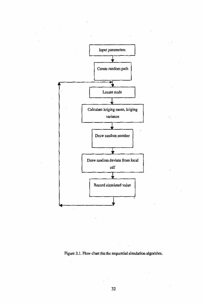
a set of Fortran programs. The flowchart shown in Figure 3.1 outlines the steps
involved in the sequential simulation algorithm discussed in Section 3.1. The main
difference between the simulation algorithms is associated with the subroutine in
which a random deviate is drawn from a local conditional distribution.
31
Input parameters
• Create random path
-:Y_
Locate node
,1. Calculate kriging mean, kriging
variance
• Draw random number
... Draw random deviate from local
cdf
+ Record simulated value
~ -
Figure 3.1. Flow chart fonthe sequential simulation algorithm.
32

3.8.1 Sequential Gaussian simulation-SGSIM
The SGSIM algorithm used the program sgsim. exe from the Geostatistical Software
Library (GSLIB). The only modification that was required to run this program was
an adjustment to the dimension of some matrices, since the Penneability data set
was larger than the preset default values. The parameter files for the Permeability
and Potassium data sets are included in Appendices AI and Bl respectively. The
program requires a semivariogram model for the normal scores, and the kriging
variance is directly interpreted as the variance of the conditional distribution, so
the nugget constant and the sill parameters must add to 1.0. (Deutsch & Journel,
1998).
3.8.2 Direct sequential simulation
In the case of the three direct sequential simulation algorithms we need to input
a non-standardised semivariogram model derived from the original sample data.
The programs do not require that the data be transformed to normal scores. Our
implementation is based on a modification of SGSIM. As a first step the subroutine
krige was changed to incorporate the sample mean into the formula for the kriging
mean, as SGSIM calculates the simple kriging mean using a global mean of zero.
This program will be referred to as dssim.exe. Additional requirements for the
particular direct sequential simulation algorithms were then added where necessary.
3.8.3 DSSIM - Original direct sequential simulation
This program is a modification of dssim.exe so that the local conditional probability
distribution is no longer assumed to be normally distributed. The code was amended
to allow the random deviate associated with a location to be drawn from a lognormal
distribution. The parameters for this distribution are calculated from the simple
kriging mean Wid simple kriging variance using Equations (35)-(36). The parameter
files are for the Permeability and Potassium data sets are seen in Appendices A2
and B2 respectively.
33

3.8.4 Direct seqnential simulation with histogram reproduction
The two algorithms, DSSLl and DSSL2 require a global target histogram at the
start of the programs. These histograms consist of 40 equiprobable classes with a
maximum and minimum value determined by the parameters zmin and zmax. The
thresholds and global probabilities for the Permeability and Potassium data sets are
given in Appendices A5 and B5 respectively. These programs differ from SGSIM and
DSSIM in that they make use of special subroutines which return a local probability
distribution from which a random deviate is drawn, as shown in Figure 3.2.
3.8.5 DSSLl R Direct sequential simulation with histogram reproduction
using the one-norm
For this algorithm we included Algorithm 552 from the Association for Computing
Machinery (ACM) Transactions of Mathematical Software (Barrodale & Roberts,
1980) as a subroutine in the modified dssim.exe program. The parameter file for
dssil.exe for the Permeability and Potassium data sets are given in Appendices A3
and B3 respectively. From Equations (55)-(57) the parameters listed in Table 3.1
must be passed to the Algorithm 552 subroutine at execution time.
The only parameters that are continuously updated from location to location are
C and d. The subroutine returns the solution vector through an array and a logical
flag which indicates if an optimal solution was found.
The program also requires values for the following three parameters:
• Iter - an upper bound on the maximum number of iterations allowed. It is set
to the suggested value of 10 (k + l + m). This parameter is actually calculated
in the program after k is input.
• Kode- a parameter that on exit informs the main program if an optimal solu
tion has been found. On entry though, if set equal to one, the nonnegativity
constraints on the probabilities are included implicitly in the constraints. This
has been coded into the program and no further input is required. If the flag
returned with the solution vector informs the main program that a solution
34

Call program
Alg552/ LSSOL
]. No Yes
Flag=()?
----Use returned pdf to
Set random deviate= create cdf
kriging mean • .J. Locate threshold interval corresponding
Reset flag = 0 to random number r.
• Calculate random deviate
using linear
interpolation.
Figure 3.2. Flowchart for calculating a random deviate with DSSL11DSSL2 .
35

was not folllld, the estimate is set equal to the simple kriging mean, and the
program continues.
e Toler - a small positive tolerance for which empirical evidence suggests be set
as toler= lQ(-;"') where d represents the munber of decimal digit,s of accuracy
available. The subroutine cannot distinguish between zero and any quantity
whose magnitude does not exceed toler. It will not pivot on any number whose
magnitude does not exceed toler. The tolerance is preset at a value of 10-5 in
the program code.
Table 3.1. Parameters for Algoritlun 552.
Parameter Description and input
K
L
M
N
A
c
E
b
d
f
Number of rows of matrix A = 40
Number of rows of matrix C = 3
Number of rows of matrix E = 0
Number of columns of the matrices A,C,E = 40
0
I 0 0
0 I
0 0
("i'') ("t'•)'
I
0
I
(''i'') (''i")'
1
(pj,V,,··· ,ptf
(z_9K, a~K + (z8K)2, l)T 0
36
ck-~+t~o)
ck-~+t~o)2
1

3.8.6 DSSL2- Direct sequential simulation with histogram reproduction
using the two-norm
This algorithm solves the quadratic progn.mming problem in Equation (48). In
order to accomplish this we use the software package LSSOL, version 1.0. This is
a set of Fortran subroutines for linearly constrained linear least-squares and convex
quadratic programming. LSSOL uses the two--phase, active-set type method. (Gill
et al, 1986). The reader is reierrcd to the user's guide for an in-depth discussion of
the program and parameters.
The LSSOL subroutine is included in a modified dssim.exe program. The pa
rameter files for dss£2. exe for the Permeability and Potassium data sets are given
in Appendices A4 and B4 respectively. The LSSOL program states the quadratic
programming in the general form
Minimise
(77)
subject to
(78)
where I and u are the lower (BL) and upper (BU) bounds respectively.
The program requires an initial estimate (X) of the solution be entered. The
LSSOL subroutine requires the following parameters to be input at execution time.
The only parameters that are continuously updated from location to location are
C, BL and BU. The subroutine returns the solution vector through an array and
a logical flag which indicates if an optimal solution was found. Before calling the
lsmain subroutine with the required inputs, we call the subroutine lsoptn to select
a programming problem of type QP2.
37

Table 3.2. Parameters for LSSOL.
Parameter Description and input
M
N
NCLIN
NROWC
NROWA
c
B!,
BU
X
A
c
Nwnber of rows of matrix A = 40
Number of variables = 40
Nwnbcr of general linear constraints = 3
Row dimension of C = 3
Row dimension of A = 40
I I I
(~) (''i'') c ... -~+tk) ( ''i'' ) 2 (''i'•)' e,.-~+t,.)2
[ 0 0 0 ... 0 I zSK cr~K + (z~K )2 J
[ l l I ... 0 I • ZsK O"~K + (z,SK )2 J fuitial cst.imate = (JJJ ,~, •.. ,PJ.)T
I 0 0
0 I 0
0 0 I
(p'{,]f,, ... ,pff
38

4 Performance Assessment
Multiple realisations generated by simulation algorithms provide a measure of the
uncertainty about the spatial distribution of attribute estimates. This uncertainty
arises from our imperfect knowledge of the phenomenon under study. It is dependent
on both the data and the model specifying our prior decisions about the phenom
enon (Goovaerts, 1997). There are several ways in which the spatial uncertainty
can be assessed. Qualitative assessment includes visualisation of realisations and
various types of displays. Quantitative assessment focusses on the reproduction of
key statistics such as the target histogram and semivariogram.
4.1 Qualitative Assessment
For each simulation algorithm, we generate a set of L realisations. These sets can
be post-processed and the spatial uncertainty can be visualised through different
displays, including probability maps, quantile maps and conditional variance.
4.1.1 Probability Maps
At each simulated grid node uj, the probability of exceeding a given threshold zk is
evaluated as the proportion of the L simulated values that exceed that threshold.
The map of such probabilities is referred to as a probability map.
4.1.2 Quantile Maps
The p-quantile of the distribution F (x) is the value Xp such that
F(xp) = Pr(X ~ x,) = p. (79)
Quantile maps display the p-quantile values corresponding to any given probability
p. In this study we will be comparing xo.bthe median xo.s and xo.9· Local differences
between realisations can be depicted through the changes in the quantile maps.
39

4.1.3 Conditional Variance
The conditional variance u2 (u) measures the spread of the conditional probability
distribution around its mean zE (u) :
a2 (u) = L: [z- z'E;(u)] 2 f (u[ (n)) dz. (80)
In practice, this is approximated by the discrete sum
K+l
a2 (u)"' L [z- zE, (u)] 2 [F (u;z. (n))- F (u; Zk-1 (n))] (81) k=l
where zk, k = 1, ... , K, are the threshold values discretising the range of variation
of z-values, Zk is the mean of the class (zk_1, Zk], which depends on the within-class
interpolation model, and zE (u) is the expected value of the conditional cumulative
dbtribution function approximated by the discrete swn
K-t-1
z;, (u)"' L z IF (u;zk(n))- F (u; Zk-1 (n))]. (82) k=l
The variance estimate in (81) depends on the K within-class means Zk. The
COnditional variance cr (u) I COnditional CUmulative distribution function mean and
upper tail mean can be very sensitive to the choice of extrapolation model. Local
differences between realisations can be depicted through mapping a measure of the
spread of the distribution of L simulated values at each simulated grid node.
4.2 Quantitative Assessment
The quality of a realisation could be defined as its ability to match a priori knowl
edge about the spatial distribution of the attributes values (Goovaerts, 2001). The
structural characteristics of a simulation, which include the histogram and the semi
variogram, are evaluated from its values at the nodes of the discretisation grid, which
differ from the characteristics of the theoretical model or the sample data. (Chiles
& Delfiner, 1999).
The performance of the simulations can be checked both visually and quanti
tatively by comparing the histogram and the semivariogram reproduction for each
40

realisation. These allow us to calculate the fluctuation variance of the spatial mean
of the simulation and, in the Gaussian case, the spatial variance of the simulation
and of its variogram. This enables us to see if the deviations of these characteristics
from their theoretical values are acceptable.
4.2.1 Histogram Reproduction
Two quantitative measures used to compare the target histogram and the histogram
of the realisations is given by the mean absolute deviation (MAD) and the mean
squared deviation (MSD) between the target quantiles and the quantiles of the
realisation. If there are K classes the mean absolute deviation is given by
E jz,- z)'l j H ~·-='1'---=--MAn= K
and the mean squared deviation as
K ( .(£))2 I: Zi-Zi i=l
HMsv= K
(83)
(84)
where Zi and Zi denotes the ith quantile of the target distribution and the fth re
alisation respectively. When the mean squared deviation is very large, the natural
way to reduce the magnitude of the measure is to take the square root. The mag
nitude of the discrepancies between realisation and model statistics are referred to
as ergodic fluctuations and they depend on several factors, including the density of
the conditioning data, the semivariogram parameters and the size of the simulation
grid.
Both measures of accuracy are used in comparing the histogram reproduction for
the simulation algorithms as the mean average deviation is comparative to DSSLl
and the mean squared difference is comparative to DSSL2. By considering both
measure we can eliminate any bias towards a particular algorithm.
41

4.2.2 Semivariogram Reproduction
To compare the semivariogram of the realisations with the theoretical model we
calculate the mean square deviation between the theoretical model and the exper
imental semivariogram values. For an isotropic data set, this is done by using an
omnidirectional model and omnidirectional expedrr:.ental semivariogram for each re
alisation and the mean squared deviation is given by
L 2 L: (7 (h;)- 'i (h;)) MSD1 = :c:;~"-1----;---
L (85)
where l1i denotes the ith lag vector, L denotes the number of lags and 'Y and .:Y
denote the theoretical semivariogram and the experimental semivariogram of the
realisation respectively.
"When the data set is anisotropic we sum the mean squared deviation in the
directions of maximum and minimum continuity. This mean squared deviation is
given by
where 'Yma.x and 'Ymin are the experimental semivariograms in the directions of max
imum and minimum continuity respectively. When the mean squared deviation is
very large, the natural way. to reduce the magnitude of the measure is to take the
square root.
42

5 Application to the Isotropic Case
The Permeability data set comes from Goovaerts (2001) and consists of of perme
ability values in a 2-D section of a reservoir. The 10404 data measurements are
located on a 102 x 102 regular grid which has a grid spacing of 1.0 unit. The sam
ple set Perm50 also comes from Goovaerts (2001) and consists of fifty permeability
values randomly drawn from Permeability.
5.1 Exploratory Data Analysis
Descriptive statistics for the permeability variable from Permeability and Perm50
are listed in Table 5.1.
Table 5.1. Descriptive statistics for the Permeability and Perm50 data sets.
Permeability Perm50
n 10404 50
Mean 582.95 592.53
Std Deviation 502.5 481.653
Variance 252502 231989
Skewness 1.265 1.184
Kurtosis 1.370 1.417
Minimum 1.03 4.47
1st quartile 194.21 194.28
Median 480.69 576.30
3rd quartile 869.17 853.42
Maximum 2498.87 2081.85
IQR 674.96 659.14
!Umge 2497.84 2077.38
The data sets have similar means and standard deviations, but there is a notice
able difference in minimum, median and maximum values. The sample data have a
higher minimum and median and a lower maximum than the exhaustive data. The
43

positive skewness evident in the histograms, and seen in Figure 5.1, is confirmed by
the summary statistics, but overall the sample data appear to reflect the smnmary
statistics of the exhaustive data. Neither set is normally distributed.
0.25
0.2 .. g 0.15 Cll = 1:1" ~ 0.1 ~
0.05
0 0
Permeability 0.25 Perm50
0.2 .. " 0.15 I: Cll = 1:1" Cll 0.1 li:
0.05
0 400 800 1200 1600 2000 2400 0 400 800 1200 1600 2000 2400
Permeabilit' Permeabilit'
Figure 5.1. Histograms for· Permeability (left) and Perrn50 (right).
There are several extreme values in the data sets. The maximum Permeability
and P erm50 values are approximately equal to fom times the mean. These extreme
values will influence the simple kriging means. These values are sometimes deleted
from a sample data set or adjusted to reduce their influence, but since they originated
from an exhaustive data set, they must be incorporated into the analysis in this case.
The cumulative frequency distributions and the Q-Q plot comparing the exhaus
tive and sample permeability data sets are shown in Figure 5.2.
Q-Q Plot 2500
2000
~- 4 0 1500 o,n E ... Q) 1000
1:1. ;. .... • 500 .0!-•..
~· • 500 1000 1500 2000
Permeability
Ci' c: ~ 0.8
ii-Q) ... O.G u.. ., .!: M ~ :::0
02 § (j
2500
Cumulative Frequency Distribution
-+- Permeability -+- Perm50
500 1000 1500
Permeability 2000 2500
Figure 5.2 Q-Q plot (left) and cumulative frequency distribution (right).
We notice the cumulative frequency cmves arc almost identical to begin with
and then there are some deviations in their shapes. The sample does not contain
44

the extreme high values present in the exhaustive data set, but the fit is reasonably
good considering the sample size is relatively small.
The forty permeability thresholds are used to define the global probability distri
bution in DSSLl and DSSL2 are given in Appendix A5. These values are bounded
by a minimum value of 1 and a maximum value of 2500. For each simulation we will
consider the conditional cumulative frequency function at two locations u 1 ( 46, 94)
and u2(88, 52) whose exact values are known to be 421.02 and 26.11 respectively.
Location u 1 is situated in a sparsely sampled region of above average values and
location u2 is situated in close proximity to three low values.
Figure 5.3 shows plots of the permeability values for Permeability and Per-rn50.
The sample data are randomly located within the study region. The Perm50 data
are sparsely situated in the southern and north-eastern regions and do not capture
the spread of high values evident in the exhaustive Permeability data.
N Pe~so 0
00 ,- • 0(1 120 0 1""1 1 ~[I (10'1 1QO 0r 1 • • 11:1001""1 200 OCJ Z50000 IJ • • :::00 000
2eoocn 490 000 • • • 490 000 t:'OO 000 • • • • • 600000 780 0 00 ..... • • • • 78 0000 880 000 IJ.1 • 880000 • • • 1340 OL10 •• • 1340.000 2000.000 • • 2000.000 2500.COO 2500.000 • • • •
• 0 • • • ~
0 5 1 102
Figure 5.3. Plots of permeability values for Permeability (left) and Perm50 (right).
5.2 Variography
The direct simulation algorithms we investigate all make use of simple kriging, and
for this to be applied we must first calculate an experimental semivariogram and fit
an appropriate model. The direct sequential simulation algorithms do not requn:e
the data to be transformed, but in order to apply sequential Gaussian simulation
the Perm50 data must first be transformed to obtain standard normal scores. The
45

variogram surfaces from Perm50 and the Perm50 Normal Scores data sets were
created using 4 lags with a lag spacing of 10 and are shown in Figure 5.4. There
appears to be no strong evidence of anisotropy evident in either data set, so an
isotropic model was fitted in both instances.
0 Perm50 Variogram Surface
0 Perm50 Normal Scores Variogram Surface
<:t <:t 0 .0
0
soooo.ooo 0.2SO 1.ooo .... os o.soo 1 .SOOcz .. OS 0. 7 SO
2 .OOOcz .. OS 1 .000 2 .SOOcz .. OS 1 .2SO 3.ooo .... os o 3.soo .... os 4.ooo .... os 4.soo .... os •
1 .SOO 1.7SO
2 .000
0 ~+-----~--r-------~
0 ~T---------r-----~~
-40 0 40 -40 0 40
Figure 5.4. Variogram surface for Perm50 and Perm50 Normal Scores.
T he omnidirectional experimental semivariogram for Perm50 was calculated us
ing 12 lags at a lag spacing of 5.5. The fitted model and its parameters are shown
in Figm e 5.5 and Table 5.2 respectively. T he model consists of a nugget effect and
two spherical structures. The contribution of the nugget is approximately 19% of
the total sill and the two spherical structures have ranges of 10 and 50 respectively.
YCihl) Omnidirectional 270000 •
• 240000 -------2 10000 • • • 180000 • 150000 • 120000 • 90000
60000
30000
0 0 7 14 21 28 35 42 4Q 56 63
Jhl
Figure 5.5. Omnidirectional experimenLal semivariogram model for Perrn50.
46

Table 5.2. Omnidirectional semivariogram model for Penn50,
1st Structure 2nd Structure 3rd Structure
Type Nugget Spherical Spherical
Range 10.0 50.0
Sill 43680 63000 124000
The omnidirectional experimental semivariogram for the Perm50 Normal Scores
was calculated using 8 lags at a lag spacing of 10 and its parameters are given in
Table 5.3. The model is shown in Figure 5.6 and it consists of a nugget contributing
14% of the total sill and one spherical structure with a range of 24.
7CI•D Omnidirectional • • • ----- • ,. •
00
0.4
" 0
0 • " 24 .. ., .. " "' 72 .. ,., Figure 5.6. Omndircctional semivariogram model for Perm50 Nonnal Scores.
Table 5.3. Omnidirectional semivarigram model for Perm50 Normal Scores.
Type
Range
Sill
1st Structure 2nd Structure
Nugget
0.14
47
Spherical
24.0
0.86

5.3 Simulation
The Permeability data set is positively skewed, so when using SGSIM, the lower tail
is extrapolated using a negatively skewed power model with w = 2.5 and for the
upper tail a hyperbolic model with w = 2.0. The cumulative frequenccy distribution
for Permeability, shown in Figure 5.2, has a relatively long tail, and we do not
want to understate the probability of occurrence of very large values. The minimum
value for the permeability values is set to 1. The DSSIM algorithm does not have a
maximum value set but the other algorithms have their maximum value set to 2500.
The positive skewness visible in the Permeability data set suggf'..sts considering a
lognormal local conditional distribution, by transforming the mean and variance of
the data using Equations (35)-(36).
To reduce computational effort, the conditioning data is locatOO within a neighM
bourhood of the location being simulated. At least four and at most twenty origiM
nal data values, ar._i up to twelve simulated values are used in each simulation. A
multiple-grid concep~ is used, whereby a coarse grid is simulated first and then used
to condition a second, finer grid simulation. The grid refinement is performed three
times and this results in better reproduction of the long range variogram structure.
The random number generator draws independent seed values uniformly distrib
uted in [0, lJ. Each realisation is identified by its random number seed, and this
number remains the same for each simulation algorithm. This means, for example,
that realisation #1 using SGSIM was generated using the same random path as
realisation #1 using DSSIM. For each algorithm we generate 100 realisations.
In Figure 5.7 and Figure 5.8 we compare the mosaic maps for the realisations with
the minimum, median and maximum mean absolute deviation and mean squared
deviation from the Permeability data set respectively. The realisations with the
maximum deviations are the same for both accuracy measures for all simulation
algorithms except DSSLI. The realisations with the minimum deviations are the
same for both accuracy measures when using DSSIM and DSSL2. There does not
appear to be any significant differences between the corresponding realisations of
the different measures.
The SGSIM and DSSIM algorithms appear to overestimate the values in most
48

O.Q 120000
u.o.ooo 200.000 2ll0.000 .o480.000 000.000 7 90.000 980.000 1~.000
2000.000 2500.000
0 .0 120.000 190.000 200.000 2ll0.000 "180.000 600.000 780.000 880.000 1340.000 2000.000 :2500,000
0 .0 120.000
190.000 200.000 260.000 -180.()(X)
000.000 780.000 880.000 13'*0.000 2000.000 2500.000
N PERM50 ~
I, •
•
"'
0 . 0 5 1
g SGSIM (MAXIMUM, 1100) MAD ..... · ... 0 .0
120 .000
0
g DSSIM (MAXIMUM, 134) MAD
0 51 102
00 120 000 190.000 200.000 2<10.000
"8 0 .000 600 000 . 7 8 0.000 . 880 .000 1340.000 2000.000 2500.000
102
190.000 200 .000 260.000 480 .000 600.000 780 .000 880.000 1340.000 2000.000 :2600.000
00 120000 100.000 200.000
2 60.000 4SOJJOO
600.000 780.000
880.000 13~0.000
2000.000 2000.000
0 .0 120.000 190.000 200.000 260.000 "180.000 600.000 780.000 880.000 1340 .000 2000.000 2500.000
00 120 000
100.000 200.000 2!10.000 "180.000 000.000 780.000 880.000 1340.000 2000.000 2500.000
Figure 5.7 . Post plots for realisations with mm1mum, median and maxrrnum mean absolute
deviation.
49

g SGSIM (MINIMUM, 145) MSD ,r
g OSSL2 (MINIMUM, 139) MSO
0.0 120.000 IQOOOO
200.000 2<!0.000 •eo ooo 000.000 790000 880.000 13<W.OOO 2000000 2~.000
0 0 120.000 1 00 000 200.000 2<10.000 480 000 000.000 790.000 880.000 13-40.000 2000000 2<500.000
0 .0 120 .000 100 000 200.000 >eo.OOO 480 000 000.000 700.000 880.000 1340.000 2000000 2<500000
iti
0
iti
0
00 120000 100000 200.000 2<!0.000 480 000 000.000 790 000 180.000 13 4 0 .000 2000 000 2GOO.OOO
00 120.000 UIO.OOO
200.000 2<10.000 480 000 000.000 790 000 880.000 1310.000 2000000 2<500.000
00 1 20.000 1QO.OOO
200.000 2(5().000
480 000 000.000 700.000 880.000 13 .. 0 .000 2000000 2<500.000
"' PERMSO 0 ~
I' •
iti
0 . 0
• 51
00 120.000
100000 200.000 2eo.ooo 480 000 000.000 7110000 880.000
13<10.0CXJ
2000000 2COO.OOO
0 .0 1 20 .000
100000 200.000 2e0.000 480 000 000.000 790.000
880.000
1340 .000
2000000 2000 000
g SGSIM (MAXIMUM, 1100) MSD ~ 00
g DSSIM (MAXIMUM, 134) MSD
. . . ·.
iti
0
102
00 120.000 1110000 200.000 2<!0.000 •ao ooo 000.000 780 000
880.000 13-40.000 2000 000 2(5()().000
120,CX)Q
1110000 200.000 2<10000 •so ooo 000.000 700 000 8010.000 1340 .000 2000000 2GOO.OOO
00 120 000 1til0.000
200 000 280.000 480 000 000.000 790 000 880.000 1310.000 2000000 2<500.000
0 0 120.000 190000 200000 >CIOOOO
•eo ooo 000.000 780 000 aao ooo 1310 .000 2000000 2500.000
g OSSL2 (MAXIMUM, 130) MSD 'I"'" 0 .0
0
120.000 1110 000 200.000 200.000 .o480 000 000.000 780 000
880000 13 .. 0 000 2000000 2000000
Figure 5.8. Post plots for realisations with mmunum, median and maxtmum mean squared
deviation.
50

regions and the spatial features are not reproduced very well. The maps show that
the high regions seen in the Permeability map have not been reproduced. The algo
rithms have attempted to replicate the region of higher values in the southeast corner
and the region of low values near the central eastern border. The DSSLl and DSSL2
algorithms ropruduce the spatial features well and indicate that there are high values
in the southwe.:1t and northeast corners but they tend to underestimate the low3r
values. 'T'h~, also indicate the presence of high values in the southeastern corner
and low values near the central eastern border, There is far better reproduction of
the low values within the western half using the DSSLl and DSSL2 algorithms than
with SGSIM and DSSIM.
The region of very high values seen the the southwest corner in the Permeabil
ity map has not been reproduced by any of the simulation algorithms but this is
understandable since the this area was not sampled from. The realisations relating
to DSSL! and DSSL2 appear more disjointed and scattered than the SGSIM and
DSSIM realisations. The DSSIM realisation appear to be smoother than the others,
and there seems to be a lot of locations with values closer to the mean.
5.4 Histogram Reproduction
The histograms for the realisations with the best, worst and median reproduction
are shown in Figure 5.9. The SGSIM realisations match closely to the Perm50
distribution, but they do not reproduce the Permeability distribution. The DSSIM
realisations are influenced by the local conditional distribution used in the simulation
process, and this lognormal distribution is clearly evident in the graphs. As the mean
absolute deviation increases there is a noticeable change in the shape of the DSSIM
distributions. The distribution of the realisation with the maximum deviation
appears to be almost normally distributed. The distributions for DSSLl and DSSL2
are very similar and both reproduce the Penneability distribution very well. The
large spikes of low values are due to the random deviate being set equal to the simple
kriging mean when the algorithms fail to find a solution. This problem occurs when
the simple kriging mean is less than the midpoint for the first global probability
threshold. The spike increases in size as the mean absolute deviation increases.
51

03
g 02 ., :I
~ .._ 0 I
0
03
g 02
~ .,. ~ 01 ...
0
03
,.. u ii :I
02
.,. ~ ... 01
0
03
,.. ~ 02
.,. ~ 01 ...
0
SGSIM (MINIMUM, 1137) MAD 03
,.. 02
~ .,. ~ 01
0
SGSIM (MEDIAN, 1117) MAD 03 SGSIM (MAXIMUM, 11100) MAO
~ 0 2
~ :I .,. f 0 1 ...
0 0 400 800 1200 1600 2000 2400 0 400 800 1200 1600 2000 2400 0 400 800 1200 1600 2000 2400
Permeability
OSSIM (MINIMUM, #60) MAD
Permeability
0 3 DSSIM (MEDIAN, 1131) MAD
~ 02 0::: ., :I g-~ 01
Permeability
03 DSSIM (MAXIMUM, 1134) MAD
~ 02 0::: .. " .,. ., ~ 01
0 400 800 1200 1600 2000 2400 0 • 400 800 1200 1600 2000 2400
Permeability 400 800 1200 1600 2000 2400
Permeability
0
0
Permeability
0.3
"' 02 g ~ .,. ~ .._ 0 I
PERMEABILITY
400 800 1200 1600 2000 2400 Permeabilily
03
~ 02
iii " ~ ... 01
PERM 50
400 800 1200 1600 2000 2400
Permeablity
DSSU (MINIMUM, 114) MAD DSSLl (MEDIAN, 1113) MAD OSSL1 (MAXIMUM, 1157) MAD
03 03
"' ,.. u u 0::: 02 0::: 02 ~ .. :I
.,. .,. Q)
~ ~ OJ ... 0 1
0 0 0 400 800 1200 1600 2000 2400
400 800 1200 1600 2000 2400 400 BOO 1200 1600 2000 2400
Permeability Permeability Permeability
OSSL2 (MINIMUM, 1139) MAD DSSL2 (MEDIAN, 1199) MAD OSSL2 (MAXIMUM, #30) MAD
03 03
,.. ,.. u u ii 02 0::: 02
Q)
" :I .,. .,. ~ .. ... 01 ~ 01
0 0 400 600 1200 1600 2000 2400 0 400 800 1200 1600 2000 2400 0 400 800 1200 1600 2000 2400
Permeability Permeability Permeability
Figure 5.9. Histograms for minimum, median and maximum mean absolute deviation.
52

,., u
" .. :J cr .. .::
0.3
02
0.1
SGSIM (MINIMUM, #45) MSD
400 800 1200 1600 2000 2400
Permeabilily
o.J DSSIM ( MINIMUM, #60) MSD
,., 02 g " :J cr
" ~ 0.1
... 800 1200 1600 2000 2<00
Permeability
0.3
,., u
" 02 ..
:J
Z" .:: 0.1
SGSIM (MEDIAN, #64) MSD
400 800 1200 1600 2000 2400
Permeability
o.J DSSIM (MEDIAN, #44) MSD
g 0.2 .. ~ u.. 0.1
... 800 1200 1600 2000 2<00
Permeability
0.3
,., 02 u
" .. :J cr .. .:: 0.1
0.3
~ 02
" " :J cr
" ~ 0.1
PERMEABILITY PERM 50 0.3 0.3
,., 02 02 g ~ " l 0 1
:J cr ~ 0.1 ...
SGSIM (MAXIMUM, #100) MSD
400 800 1200 1600 2000 2400
Permeability
DSSIM (MAXIMUM, #34) MSD
400 800 1200 1600 2000 2400 Permeability
400 800 1200 1600 2000 2400
Permeability
400 800 1200 1600 2000 2400
Permeablity
,., u
" .. :J cr
" .::
0.3
02
0.1
DSSL1 (MINIMUM, #23) MSD
400 eoo 1200 16oo 2ooo 24oo
Permeability
DSSL2 (MINIMUM, #39) MSD
,., u
0.3
; 0.2 :J g-~ 0.1
400 800 1200 1800 2000 2400
Permeability
"' u c;
" :J cr ~ ...
0.3
02
0.1
DSSL1 (MEDIAN, #92) MSD
400 800 1200 1600 2000 2400
Permeability
DSSL2 (MEDIAN, #13) MSD
0.3
0.2
0.1
400 800 1200 1600 2000 2400
Permeability
DSSL1 (MAXIMUM, #65) MSD
0.3
02
0.1
400 800 1200 1600 2000 2400 Permeability
DSSL2 (MAXIMUM, #30) MSD
0.3
0.2
0.1
400 BOO 1200 1600 2000 2400
Permeabili ty
Figure 5.10. Histograms for minimum, median and maximum mean squared deviation.
53

Figure 5.10 compares the probability distribution functions for the realisations
with the minimum, median and maximum mean squared deviation. The SGSIM
realisations again match closely to the Perm50 distribution and they do not match
the Permeability distribution. The DSSIM realisations are influenced by the local
conditional lognormal distribution with relatively smooth distributions. The DSSLl
and DSSL2 distributions are very similar and the low value spikes are noticeable.
The reproduction of the Permeability distribution is evident.
For the SGS!M algorithm realisation #100 has the worst match with the global
distribution for both. The choice of measure does not have a significant effect on
the SGSIM distributions. The DSSIM distributions are noticeably different for the
realisations with both minimum and maximum deviations. There does not appear
to be a significant difference in the DSSLl and DSSL2 realisations between the
different measures of accuracy. The spike of low values appears to be slightly lower
for the DSSLl realisations using the mean squared deviation rather than the mean
absolute deviation.
From Table 5.4 we see that for the realisations with the minimum mean absolute
deviation, the DSSL2 algorithm appears to perform better, but when we look at
those with the median and maximum mean absolute deviation, the DSSIM algorithm
provides a better fit to the Permeability data set.
Table 5.4. Mean absolute deviation between realisation and target distribution.
Histogram MAD SGSIM DSSIM DSSL1 DSSL2
Rank # MAD # MAD # MAD # MAD
Minimum 37 53.47 60 41.51 4 49.79 39 33.70
Median 17 87.28 31 75.79 13 96.99 99 88.05
Maximum 100 170.00 34 158.91 57 183.10 30 207.51
A similar result is seen in Table 5.5 when comparing the realisations using the
mean squared deviation. The difference between the two deviation methods is seen
in the realisations with the median deviations. For the mean absolute deviation we
find DSSIM <SGSIM<DSSL2<DSSL1 but for the mean squaxed deviation the order
54

has changed to DSSIM<DSSL2<DSSL1<SGSIM. The DSSLl performs better than
the DSSL2 algorithm for the realisations with the minimum and median deviations.
Table 5.5. Mean sqared deviation between realisation and target distribution.
Histogram MSD SGSIM DSSIM DSSLl DSSL2
Rank # MSD # MSD # MSD # MSD
Minimum 45 79.03 60 52.26 23 67.53 39 45.17
Median 64 128.46 44 99.; 92 124.04 13 106.30
Maximum 100 203.48 34 176.81 65 213.60 30 234.65
Table 5.6 and Table 5.7 compare the realisations with the minimum mean ab-
solute deviation and the mean squared deviation respectively. For DSSLl and
DSSL2, the median values are higher and the lower quartiles are less than the target
values. The upper quartile for SGSIM with both accuracy measures is significantly >
lower than the upper quartile for Permeability.
Table 5.6. Comparison of realisations with minimum mean absolute deviation.
Minimum MAD SGSIM DSSIM DSSL1 DSSL2 Permeability Perm50
Mean 556.24 588.19 542.52 570.63 582.95 592.53
Std Deviation 520.47 500.73 495.70 517.48 502.5 481.65
Skewness 1.45 1.06 1.05 1.23 1.26 1.18
Minimum 1.84 1.00 1.00 1.00 1.03 4.47
1st quartile 192.80 187.27 127.51 174.97 194.21 194.28
Median 469.76 476.76 496.90 503.56 480.69 576.30
3rd quartile 794.00 867.67 866.35 870.32 869.17 853.42
Maximum 2500 3559.29 2498.92 2497.78 2498.87 2081.85
No restriction was placed on the maximum value for the DSSIM algorithm and
this value is very high. The SGSIM has a higher standard deviation than Perme
ability when using the mean absolute deviation, but when using the mean squared
deviation the standard deviation is less. Compared to Perrneability1 both DSSIM
and DSSL2 have a lower degree of skewness for both accuracy measures.
55

Table 5.7. Comparison of realisations with minimum mean squared deviation.
MinimumMSD SGSIM DSSIM DSSLJ DSSL2 Permeability Perm50
Mean 557.90 588.19 553.67 570.63 582.95 592.53
Std Deviation 446.91 500.73 492.!3 517.48 502.5 481.65
Skewness 1.35 1.06 1.00 1.23 1.26 J.J8
Minimwn 2.00 1.00 !.OJ 1.00 1.03 4.47
1st quartile 194.31 !87.27 !37.06 174.97 194.21 194.28
Median 562.02 476.76 525.43 503.56 480.69 576.30
3rd quartile 785.01 867.67 870.81 870.32 869.17 853.42
Maximum 2500 3559.29 2499.82 2497.78 2498.87 2081.85
There are quite a few differences between the realisations with the median mean
absolute deviations and median mean squared deviation, seen in Table 5.8 and Table
5.9. The most significant difference is with the lower quartile values where DSSLl is
markedly less than Permeability when we use the mean absolute deviation. Although
not quite as low, the lower quartile value for DSSL2 is also significantly less than
for Permeability with both accuracy measures.
Table 5.8. Comparison of realisations with median mean absolute deviation.
Median MAD SGSIM DSSIM DSS!,J DSSL2 Permeability Perm50
Mean 614.81 600.16 483.55 497.22 582.95 592.53
Std Deviation 479.32 433.22 473.22 487.96 502.5 481.65
Skewness 1.37 0.80 1.21 1.36 1.26 J.J8
Minimum 2.61 1.00 1.03 1.02 1.03 4.47
1st quartile 198.19 259.66 57.51 101.31 194.21 194.28
Median 585.54 541.05 324.51 327.25 480.69 576.30
3rd quartile 841.35 865.26 763.03 8!9.11 869.!7 853.42
Maximum 2500 3327.74 2495.29 2499.37 2498.87 2081.85
The median values are also lower for DSSLl and DSSL2 when using the mean
absolute deviation, and DSSL2 is also lower when using the mean squared deviation.
The SGSIM: values are significantly higher than those for Permeability for both
56

measures. The DSSIM realisations are not a<> skewed as the target distribution
of the other realiastions generated by the other algorithms. Again we notice the
DSSIM realisations have very high maximum values. All realisations, except for
SGSIM when using the mean squared deviation, have a lower standard deviation
than Pe1meability.
Table 5.9. Comparison of realisations with median mean squared deviation.
Median MSD SGSIM DSSIM DSSL1 DSSL2 Permeability Perm50
Mean 635.24 557.76 528.53 493.81 582.95 592.53
Std Deviation 517.80 401.38 474.32 491.53 502.5 481.65
Skewness 1.28 0.87 1.11 1.36 1.26 1.18
Minimum 2.05 1.00 1.00 1.03 1.03 4.47
1st quartile 195.11 240.96 156.4.4 104.22 194.21 194.28
Median 593.64 496.35 492.93 283.60 480.69 576.30
3rd quartile 865.27 795.96 846.61 807.29 869.17 853.42
Maximum 2500 2988.07 2494.21 2499.09 2498.87 2081.85
The summary statistics for the realisations with the maximum mean absolute
deviation and maximum mean squared deviation are given in Table 5.10 and Table
5.11 respectively.
Table 5.10. Comparison of realisations with maximum mean absolute deviation.
Maximum MAD SGSIM DSSIM DSSL1 DSSL2 Permeability Perm50
Mean 711.36 709.97 398.18 375.29 582.95 592.53
Std Deviation 449.30 425.24 428.36 415.05 502.5 481.65
Skewness 0.96 0.64 !.52 1.68 1.26 1.18
Minimum 1.65 1.00 1.01 1.01 1.03 4.47
lst quartile 369.75 382.90 37.15 49.21 194.21 194.28
Median 724.26 668.65 203.55 196.17 480.69 576.30
3rd quartile 874.07 983.12 643.59 607.66 869.17 583.42
Maximum 2500 3136.33 2498.34 2494.34 249P.87 2081.85
57

Table 5.11. Comparison of realisations with maximum mean squared deviation.
MaximumMSD SGSIM DSSIM DSSL1 DSSL2 Permeability Perm50
Mean 711.36 709.97 472.70 375.29 582.95 592.53
Std. Deviation 449.30 425.24 454.40 415.05 502.5 481.65
Skewness 0.96 0.64 1.25 1.68 1.26 1.18
Minimum 1.65 1.00 1.00 1.01 1.03 4.47
1st quartile 369.75 382.90 64.59 49.21 194.21 194.28
Median 724.26 668.65 334.72 196.17 480.69 576.30
3rd quartile 874.07 983.12 737.95 607.66 869.17 583.42
Maximum 2500 3136.33 2495.16 2494.34 2498.87 2081.85
The SGSIM and DSSIM realisations have much greater means than the target
distribution, whereas those from DSSLl and DSSL2 have significantly lower means.
This also appears to be the case with the lower quartile values, medians and upper
quartile values. The SGSIM, DSSIM and DSSL2 algorithms have the same realisa
tion with maximum mean absolute deviation as maximum mean squared deviation.
The SGSIM and DSSIM realisations are not as skewed as the Permeability data set.
The cumulative distributions for the mean absolute deviation and the mean
squared deviation are shown in Figure 5.11 and they indicate that DSSLl and DSSL2
better represent the cumulative distribution function of the target distribution. The
deviation in the lower half of the SGSIM and DSSJM distributions is significant,
although the SGSIM realisation with the minimum deviation has a very good fit
to the target distribution. There is very little difference between the two accuracy
measures for DSSL2. The target cumulative distribution function for DSSLl is well
reproduced for the lower values when the mean absolute deviation is compared.
The greatest deviation for DSSLl and DSSL2 for the realisations with the smaller
deviations, is seen in the upper quartile region.
Looking at the cumulative distributions for both the mean absolute deviation
and the mean sqared deviation, and taking into accoWlt the difference between the
best and worst fitted realisations, the DSSLI algorithm appears to result in the best
histogram reprodUction.
58

0.8
~ 0.6 :0 "' .0 0 0.4 n:
0.2
0.8
~ 0.6 :0 "' .0 0
n: 0.4
0.2
0.8
~ 0.6
:0
"' .0 0.4 ~ 0..
0.2
0.8
:E 0.6 :0
"' .0 0 0.4 n:
0.2
SGSIM · MAD
--MINIMUM, (137)
--MEDIAN, (017)
--MAXIMUM, (1100)
--PERMEABILITY
250 500 750 1000 1250 1500 1750 2000 2250 2500
Permeability
DSSIM · MAD
--MINIMUM, (•60)
--MEDIUM, (Ill )
--MAXIMUM, (034)
--PERMEABILITY
250 500 750 1000 1250 1500 1750 2000 2250 2500
Permeability
DSSLl· MAD
--MINIMUM, (187)
--MEDIAN, (143)
--MAXI MUM, (•30)
--PERMEABILITY
250 500 750 1000 1250 1500 1750 2000 2250 2500
Permeability
DSSL2 · MAD
--MINIMUM, <•39)
--MEDIAN, <•99)
--MAXIMUM, (.30)
--PERMEABILITY
250 500 750 1000 1250 1500 1750 2000 2250 2500 Permeability
0.8
~ 0.6 :0 "' .0 0 0.4 n:
0.2
0.8
~ 0.6 :0 "' .0 0
n: 0.4
0.2
0.8
~ 0 .6
:0 "' .0 0.4 0 n:
0.2
0.8
... 0.6 = :g
.0 0 0.4 0:.
0.2
SGSIM • MSD
MINIMUM, (145)
--MEDIAN, <•64)
--MAXI MUM, (1100)
--PERMEABILITY
250 500 750 1000 1250 1500 1750 2000 2250 2500 Permeability
DSSIM • MSD
--MINIMUM, (160)
--MEDIUM, (044)
--MAXIMUM, (034)
--PERMEABILITY
250 500 750 1000 1250 1500 1750 2000 2250 2500
Permeabili ty
DSSLl · MSD
--MINIMUM, (123)
--MEDIAN, (192)
--MAXIMUM, (.65)
--PERMEABILITY
250 500 750 1000 1250 1500 1750 2000 2250 2500
Permeability
MINIMUM, (039)
--MEDIAN, (113)
--MAXIMUM, (•30)
--PERMEABILITY
250 500 750 1000 1250 1500 1750 2000 2250 2500
Permeability
Figure 5.11. Cumulative distribution functions for nununum, median and maximum mean absolute deviation (left) and mean squared deviation (right).
59

5.5 Variogram Reproduction
The omnidirectional experimental semivariograrns are displayed together with the
semivariogram model in Figure 5.12 (left). The program used to calculate the ex
perimental semivariograms did not start at lag 0, as the semivariogram model does,
and this accounts for the difference in the graphs. The fan shape they produce
indicates that there is a wide range in sill values. As expected the SGSIM semivari
ogram model is very well reproduced, but this is calculated using the normal scores.
SGSIM appears to have a good short range coincidence of model and experimental
sernivariograms. The majority of experimental semivariograms however understate
the variability compared to the target, although the range of the target appears
to be approximately reproduced. The DSSIM model has a higher sill than all but
a few of the omnidirectional experimental seroivariograros calculated and there are
a couple of experimental semivariograms that have very large deviations from the
semivariogram model which results in a wide spread overall. The short range fit is
relatively good, although there is a tendency to understate it.
We notice with the DSSLl model that approximately seventy percent of the
omnidirectional semivariograrns understate the sill. The short range variability is
overstated with most graphs of experimental semiV'cU"iograms above the model. The
DSSLl model also has the smaller spread of sill values when compared to DSSIM
and DSSL2. The DSSL2 algorithm appears to have an overall gTeater variability.
The short range behaviour is very similar to DSSLl. Approximately half the exper
imental semivariograms overstsate the long range variability.
In Figure 5.12 (right} we compare the experimental semivariograms with the
minimum, median and maximum deviations from the target model. These graphs
show the shape of the experimental semivariogTarns more clearly. Comparing the ex
perimental semivariograrns with the minimum deviation, we notice that the SGSIM
model is reproduced the best, followed by the DSSLl and DSSL2 models. The
DSSIM algorithm has a larger spread in sill values between the omnidirectional
experimental semivariograms with the minimum and maximum deviations.
Table 5.12 confirms that overall the DSSLl and DSSL2 methods are both better
than SGSIM and DSSIM in reproducing the target semivariogTarn model, with the
60

1.2 SGSIM (normal scores)
0.8
0.6
0.4
0.2
0~~--~--~~--~--~~--~--r-~
0 3 6 9 12 15 18 21 24 27 30
350000
300000
250000
r 2ooooo
150000
100000
50000
h
0~~--,-~--~~~-r--r--r--~~--,
0
350000
300000
250000
200000
150000
100000
50000
10 15 20 25 30 35 40 45 50 55
h
DSSLl
o +--r--r-~~~,-~--~-r--r--r~
350000
300000
250000
1 2ooooo
150000
100000
0 10 15 20 25 30 35 40 45 50 55
h
DSSL2
50000
0 ~-r~~,-~--T--r--r--r~~~~
0 10 15 20 25 30 35 40 45 50 55
h
1.2
0.8
r o.6
0.4
0.2
SGSIM (normal scores)
MINIMUM (#32) ---MEDIAN (1153)
--MAXIMUM (#55) --MODEL
o+---T---,---~---r---r---r--~--~
0
350000
300000
250000
1 2ooooo
150000
100000
50000
5 10 15 20 25 30 35 40
h
DSSIM
MINIMUM,(# 72) ---MEDIAN,(# 59)
--MAXIMUM, (#62) --MODEL
0~-r--r--r--r--r~~~~--~~--~
350000
300000
250000
1 2ooooo
150000
100000
50000
350000
300000
250000
200000
150000
100000
50000
0 5 10 15 20 25 30 35 40 45 50 55
0
0
h
DSSLl
MINIMUM, (#75) --MEDIAN, (#25)
--MAXIMUM, (#20) --MODEL
10 15 20 25 30 35 40 45 50 55
h
DSSL2
- MINIMUM,(#97)--MEDIAN,(#61)
--MAXIMUM,(# 4) --MODEL
10 15 20 25 30 35 40 45 50 55
h
Figure 5.12. Omnidirectional experimental semivariograms for 100 realisations (left) and with minimum, median and maximum mean squared deviation (right).
61

DSSLl algoritlun fitting better than DSSI.J2, since it is more central to the fan of
omnidirectional experimental semivariograms.
Table 5.12. Comparison of mean squared deviation for experimental semivariograms.
Semivariogram SGSIM DSSIM DSSLI DSSL2
l:Umk # MSD # MSD # MSD # MSD
Minimum 32 O.QJ 72 3788.8 75 8965.2 97 9288.8
Median 53 0.09 59 25686.4 25 94!3.0 61 22097.5
Maximum 55 0.25 62 105915.8 20 62951.3 4 71623.6
5.6 Spatial Uncertainty
The quantile plots in Figure 5.13 display the rmccrtainty in the simulated values.
The DSSLl, DSSL2 and to a lesser extent DSSIM, have dark blue sections nem the
central eastern border in the 0.9-quantilc maps. These areas indicate that there is
a high degree of certainty in the simulated values being low values. The DSSIM
algorithm does not indicate this area.
WheJl comparing the 0.1-quantile and 0.9-quantile maps, the cimulated values
generated using the DSSllvl algorithm have a lower degree of uncertainty, as they
have the greatest difference in values. The highest degree of tmcertainty appears
to arise when the SGSIM algorithm is mwd. 111e remits for DSSIJl and DSSL2
alguriUmts arc very similar to each other.
Two grid nodes were selected from regions displaying different spatial uncertainty
to compare the parametric and non-parametric algorithms. The true permeability
values at locations u 1 = {88,52) and u 2 = (46,94) arc 26.11 and 421.02 n::~pectively
and these are represented by the dashed lines in Figure 5.11.
62

g SGSIM (p=0.5) 00
~ SGSIM (p=0.9)
120.000 120.000 , .., 000
:>00 000 200.000 480000 eoo.ooo
iO 780 000 iO 880 .000 1340 000 2000000
2&Kl.OOO 2000 000
0 0
0
Figure 5.13. Mosaic plots comparing the 0. 1-decile, 0.5-decile and 0.9-decile.
63
00 120.000
'"" 000 200.000 280.000 480000 eoo.ooo 790.000 880.000 1340,000
2000000 2<500.000
00 120.000 190.000 200.000 2<10.000 480000 000.000 790.000
880.000 1340.000 2000 000 2!500.000
0.0 120.000 190000
200.000 200.000 480 .000 000.000 790.000 880.000 13'fO.OOO 2000000 2000.000
0 0 120.000
'"" 000 200.000 200.000 480.000 000.000 700 000
880.000 13-40 .000 2000000 2000.000

1.0
0.8
Conditior~al CDF Models at ud88,52)
--SGSIM --DSSIM --DSSLI - DSSL2
400 800 1200 1600 2000 2400 2800 Permeability
1 .0
0.8
~ 0.6 :s "' .Q 0 0.4 .. 0.
02
0.0 0
Conditional CDF Models at ux=(46,94)
--SGStM --DSSIM
--DSSL1
DSSL2
500 1000 1500 2000 2500
Permeability
Figure 5.14. Local conditional cumulat ive distributions.
At location u 1 there is a greater difference between the uncertainty models than
at location u 2 . The SGSIIvi model is controlled by the kriging variance which is
related to the distance the location is from neighbouring sample data, and this has
a greater spread at location u 2 than location u 1 which is close to sample data. The
DSSIM model has a large spread of values at both locations.
The conditional variance for each algorithm is displayed through mosaic maps
in Figure 5.15.
0 ,J(J.II ,A)
I QC(i;e~
1~···...Q!:,. - Ot."'·~ .._~l\J·..l~
llM• .... )6
l 5U'.J• ..I.Z,
•Lt-·,·~ z.~.-"-~
" DSSIM Condttlonal Variance 0
0
Figure 5.15. Comparison of conditional variance for the algorithms.

The conditional variance is very low for the DSSIM algorithm compared to the
other algorithms. The DSSL! and DSSL2 are very similar, although there are some
regions for which the DSSL2 algorithm results in a greater variation in values. The
SGSIM algorithm has the highest variatioP in simulated values. These regions are
located in areas of higher values and where the data were sparsely sampled.
5.7 Summary for Permeability
Comparing the histogram and sernivariogram reproduction for the four algorithms,
we find that, as expected, SGSIM reproduces the variogram for the normal score
data and the histogram of the sample data set. DSSIM reproduced the local log~
normal distribution used in the algorithm, but the semivariogram model was only
reproduced well over a short range. The DSSLl and DSSL2 both reproduced the
target distribution but the DSSLl algorithm reproduced the sernivariogram model
better than all the other algorithms, so it would appear to be the better algorithm
for this isotropic case.
65

6 Application to the Anisotropic Case
The Potassium data set is a two-dimensional simulated exhaustive data set based
on soil samples taken originally from B.~ uncropped field in the Jimperding Brook
catchment region in the south-west of Western Australia (Bloom & Kentwell, 1999).
The data comprise potassium concentrations in parts per million (ppm). The 3600
data measurements are located on a 60 x 60 regular grid which has a grid spacing
of one metre. Data at one hundred locations were drawn at random and form the
sample data set KJOO.
6.1 Exploratory Data Analysis
Descriptive statistics for the potassium variable from Potassium and KJOO are listed
in Table 6.1.
Table 6.1. Descriptive statistics for Potassium and K100 data sets.
Potassium K100
n 3600 100
Mean 87.097 89.447
Std Deviation 34.703 34.416
Variance 1204.31 1184.46
Skewness 1.035 0.603
Kurtosis 1.962 0.08
Minimum 23.872 34.6
1st quartile 59.941 63.875
Median 82.470 86.85
3rd quartile 106.867 110.575
Maximum 331.978 189.0
The data sets have similar descriptive statistics, although there is a noticeable
difference in the maximum values. The sample has a significantly lower maximum
value than the exhaustive set. The positive skewness evident in the exhaustive data
histogram (Figure 6.1) is confirmed by the summary statistics. We notice the sample
66

data set. Overall, the sample data appear to reflect the summary statistics of the
exhaustive data.
Pofllssium K100 0.25
0.2 0.2
.. .. f.l 0.15 f.l 0.15 c: c: & & :I :I go c:r & & 0.1 ~
0.1 ~
0.05 0.05
0 0
0 60 160 240 320 0 60 160 240 320
Potassium Potassium
Figure 6.1. Histograms· for Potassium (left) and KJ OO (right) .
There are several extreme values in the data sets. T he maximum Potassium and
K100 values are approximately fom times and twice the mean respectively. These
extreme values will inflate estimated values in their neighbomhood. The Q-Q plot
and cumulative distribution nmctions of the Potassi'um and the K1 00 data sets are
shown in Figure 6.2.
Q·Q Plot cumulative Frequency Distribution 360 / ---+
Ci' 300 c
/
~ 0.8 /
240 / tr
Ill Q /
... 0.6 Q 180 / • u. ... / Q) :s:: ... :::> 0.4
120 ./ ... ~ l":J - 0.2 60 E
' u -- Potassium --K100 0 0
0 60 120 180 240 300 360 0 60 120 180 240 300 360
Potassium Potassium
Figure 6.2. Q-Q plot (left) and cumulative frequency function (right) for Potassium and
KJOO.
Comparing the distributions we notice t hat the K100 data are representat ive of
the Potassium data. T he Q-Q plot reveals the effectiveness of the sampling. The
. 67

two distributions are ahnost identical as they follow the dashed line fail·ly closely,
the only significant exception being a single extreme value.
The forty permeability thresholds used to define the global probability distribu
tion in DSSLl and DSSL2 are given in Appendix B5. These values are bounded by a
minimum value of 20 and a maximum value of 360. For each simulation we will con-
sider the conditional cumulative frequency function at two locations u1 (28.5, 44.5)
and u 2 (28.5, 22.5) whose exact values are known to be 57.975 and 202.381 respec
tively. Location u 1 is in an area of low values and location u 2 is situated near high
values. Figme 6.3 shows mosaic plots of the potassium values for Potassium and
Kl 00. The sample data appear to have a good coverage of the study region. T he
K100 data set seems to captme the spread of high and low values evident in the
Potassium data set.
o POTASSIUM oo K100 (() 0.0 I[) 0.0
41 .000 • • •• 41 .000 56.000 • • 56.000
67.000 .....
67.000 •• 75.000 • • • 75.000 • • 89.000 • • • .. 89.000 • 97.000 .. • 97.000
0 117.000 0 • • • • • 117.000 r<J r<J • • • • 150.000 •• • • • 150.000 • • • • .. . • • • • . .. _
• • • "' ..
.• . • • • •
0 0 • 0 30 60 0 30 60
Figure 6.3. Plots of potassium values for Potassium (left) and K100 (right).
6.2 Variography
An experimental semivariogram was calculated and an appropriate model fitted so
simple kriging could be used in the direct simulation algorithms. The direct se
quential simulation algorithms do not require any data transformation, but in order
to apply sequential Gaussian simulation, the K 100 data must first be transformed
to obtain standard normal scores. The variogram surfaces of the K100 and K100
68

Nomwl Score data sets were creat ed using 7lags with a lag spacing of 3.0 and these
are shown in Figure 6.4 .
.... K100 Variogram Surface (\1
..- K100 Normal Scores Variogram Surface 0.0 (\1 0.0
200.000 0 .250
400 .000 0.500
600.000 0.750
aoo.ooo 1.000
1000.000 1.250 0 1200.000 0 1.500
1400.000 1.750
1600.000 2.000
1BOO.OOO 2.500
2.500
.... .... ~~--------~--~--_, (\1
I
-2 1 0 21 -21 0 21
Figure 6.4. Variogram surface for K100 and K100 Nor-mal Scor-es.
The data sets both appear to exhibit anisotropy, with gTeater continuity in the
N65W direction, and minimum continuity in the N25E direction. The experimental
semivariog1·ams for both data sets were calculated using 10 lags with a lag spacing
of 3. A geometric anisotropic model was fitted to the experimental semivariograms
of the K100 and K100 normal scores. In both cases, it consists of a nugget effect
and one spherical structme.
l<or K100, the nugget has a relative nugget effect of approximately 7% and the
spherical structme has a range of 22 and a nisotropy factor of 0.76. The anisotropic
model is shown in Figure 6.5 with the experimental semivariog1:ams and the parame
ters are given in Table 6.2. The model is fitted using the program Variowin and the
direction is given in degrees anticlockwise from East, so direction 65 and direction
155 relate to N25E and N65W respectively.
Table 6.2. Geometric anisotropic model for Kl 00.
Type
Range
Sill
Anisotropic ratio
1st Structw·e 2nd Structure
Nugget
84.0
69
Spherical
22.0
1104
0.76

7li•D Direction 65 •
= \lOO - - - - - -- -~-~·~--:-~-~''---"----
'D
912~1121l::<'ZI3:1 ,.,
Direction 155
1ro:l -------------~-------~-jo)) -.--- .. •
• •
9121S~~1:1o'ZI3l
" Figure 6.5. Geometric anisotropic model fitted to experimentalsetnivariogram for K100.
For KlOO, the nugget has a relative nugget effect of approximately 8% and the
spherical structure has a range of 25.0 and anisotropy factor of 0.64. The anisotropic
model is fitted to the experimental semivariogram in Figure 6.6, and the parameters
are given in Table 6.3.
""' ... ..,
Dlrtction 155
•.• --- -- -- -- =-=----;:_:::--=-~--:--:--.. "
y(llol)
••• ..,
~ " 1B 21 ~ » ~ ,.,
Direction 65
• D.g ---- - -- -:.;-;:•;.-------=------
Figur~ 6.6. Geometric anisotropic model fitted to experimental semivariogram for K100
Normal Scares.
70

Table 6.3. Geometric anisotropic model for K1 00 Normal Scores.
1st Structure 2nd Structure
Type Nugget Spherical
Range 25.0
Sill 0.08 0.92
Anisotropic ratio 0.64
6.3 Simulation
The parameter files for the simulation algorithms are listed in Appendix B. The
simulated values are located on a regular grid of size 60 x 60 and they all work
with a limited data search neighbourhood of 40.0 tmits. A minimum of four and
a maximum of twenty original sample data, and a maximum of twelve simulated
values are used in each simulation. For SGSIM, the cumulative distribution func
tion (Figure 6.2) indicates extrapolating the lower tail to the minimum value of 20,
using a linear model and the upper tail using a hyperbolic model with w = 1.5. One
hundred realisations were generated for each algorithm, and then ranked in increas
ing order according to both their mean absolute deviation (MAD) and their mean
squared deviation (MSD) from the exhaustive Potassium data set. The minimum
and maximum values, zmin and zma.x, for the potassium values are set to 20 aJid
360 respectively for SGSIM, DSSL! and DSSL2.
The positive skewness visible in the Potassium data set suggests considering a
lognormal local conditional distribution, by transforming the mean and variance of
the data using equations (35)-(36). To reduce computational effort, the conditioning
data is located within a neighbourhood of the location being simulated. At least
four and at most twenty original data values, and up to twelve simulated values are
used in each simulation. A multiple-grid concept is used, whereby a coarse grid is
simulated first and then used to condition a second, finer grid simulation. The grid
refinement is performed three times and this results in better reproduction of the
long range variogram structure.
71

The random number generator draws independent seed values unifonnly distrib
uted in [0, 1] . Each realisation is identified by its random number sred, and this
number remains the same for each simulation algorithm. This means, for example,
that realisation #1 using SGSIM was generated using the same random path as
realisation #1 using DSSIM.
6.4 Histogram Reproduction
In Table 6.4 and Table 6.5 we compare the mean absolute deviation and mean
squared deviation values for the realisations with the minimum, median and maxi
mum deviations, and from these it appears SGSIM has the closest fit to the Potas
sium data set, with DSSIM actually giving a better fit for the realisations with the
maximlUll deviatiOilll. The DSSL2 algorithm ha<i a better fit than DSSL1 except for
the maxinnun mean squared deviation.
Table 6.4. Comparison of the mean absolute deviations.
Histogram MAD SGS!M DSS!M DSSL1 DSSL2
Ranlt # MAD # MAD # MAD # MAD
Minimum 2 2.05 73 2.60 69 5.11 52 4.18
Median 7 4.28 20 5.28 90 9.10 5 8.53
Maximum 93 9.64 69 8.78 95 13.40 95 13.23
Table 6.5. Comparison of the mean squared deviations.
Histogram MSD SGS!M DSS!M DSSL1 DSSL2
Rank # MSD # MSD # MSD # MSD
Minimum 53 2.60 29 3.35 36 7.29 93 5.77
Median 5 5.12 17 5.79 64 11.13 20 10.17
Maximum 93 11.58 69 9.58 72 14.74 33 16.01
Figure 6. 7 and Figure 6.8 compare the realisations ranked according to mean
absolute deviation and mean squared deviation respectively. We notice immediately
when viewing the pootpiots that the SGSIM and DSSllvl realisations appear very
similar, as do DSSL1 and DSSI,2.
72

0
"'
. ... .. .. . · . .
0~-------:~~----~
~00
.. 1.000
""000 67.000 70.000 ag ooo 97,000 117 000 150.000
Figure 7. 7. Post plots for realisations with muumum, median and maXlillum mean absolute
deviation.
73
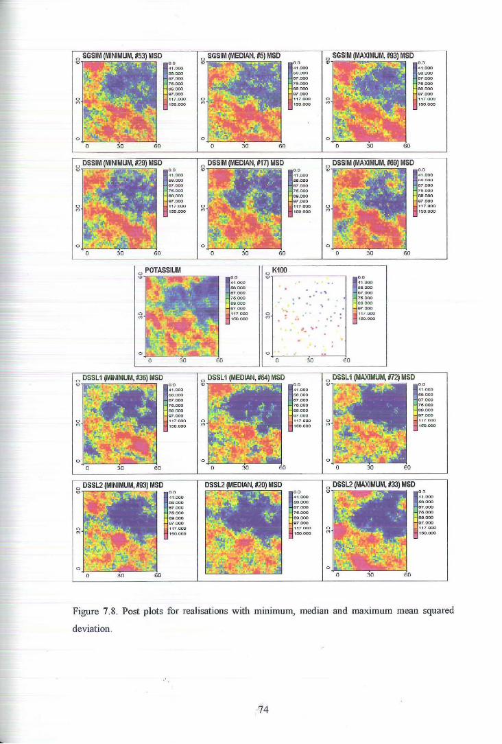
0 (')
.. ' ..
I ,
~0.0 .;1.000 56 000 07.000 7CLOOO
""000 97.000 117 000
HSO.OOO
Figure 7.8. Post plots for realisations with m1mmum, median and maxtmum mean squared
deviation.
74

There is a noticeable difference between these two distinct groups. The DSSLl
and DSSL2 realisations have a similar coverage of low values, but the values are
within the lowest interval scale. The SGSIM and DSSIM realisations appear to have
a rather large spread of high values that are well connected to each other. The high
values from DSSLl and DSSL2 are more disjointed and scattered in appearance.
Neither SGSIM nor DSSIM really capture the low values in the NE corner, but
this is not surprising since the sampling is very sparse in this region. The DSSLl and
DSSL2 realisations capture these low values best when the deviation is a maximwn.
DSSLl and DSSL2 underestimates the low values. All four algorithms seem to
recognise that there is a small area of higher values within the region of low values
near the NE corner. The high values near the centre of the region are captured
by all the algorithms, although it appears to be more evident in the SGSIM and
DSSIM post plots. It appears that SGSJM and DSSJM may overestimate the high
va]uP.s and DSSLl and DSSL2 both underestimate the high valued regions. The
anisotropy is visually evident from the mosaic maps.
The different measures of accuracy do not appear to differentiate between the
SGSIM and DSSIM algorithms. Both the mean absolute deviation and the mean
squared deviation result in realisation #93 having the maximum deviation for SGSIM.
Similarly realisation #96 has the maximum deviation for the DSSIM algorithm re
gardless of the measure of accuracy. Using the mean absolute deviation we also
notice that the realisation #95 has the maximum deviation for both DSSLl and
DSSL2.
The histograms in Figure 6.9 and Figure 6.10 highlight the differences in the
distributions of the realisations. There is very little difference between the two
accuracy measures for both SGSIM and DSSIM realisations. The DSSIM histograms
arc reproducing the :ocal conditional lognormal distribution that was used in the
simulation algorithm. Large spikes of low values are seen in the DSSLl and DSSL2
distributions and this is due to the algorithms inability to find an optimal solution
and the random deviate was set equal to a low-valued simple kriging mean. This
appears to have a significant affect on the shape of the histograms.
75

03 SGSIM (MINIMUM, #2) MAD 03 SGSIM (MEDIAN, #7) MAD 03 SGSIM (MAXIMUM, #93) MAD
C' 02
~ " !: 0 1
0
03
~ 02 c ~ " . ~ 01
0
03
g- 0.2
~ " . .:: 01
0
03
... 02 u
~ " . .:: 01
0
0 40 80 120 160 200 240 280 320
Potassium
DSSIM (MINIMUM, #73) MAD
0 40 80 120 160200 240280320
Potassium
0
03
... 02 u li t .! 0 l
0
03 POTASSIUM
~ 02
! 01
0
0 40 80 120 160 200 240 280 320
Potassium
DSSIM (MEDIAN, #20) MAD
0 40 80 120 160200240280320
Potassium
03
02
g i 01
0
~ " .
02
~ 01
0
03
... 02 u c ~
" . ~ 0 1
0
KlOO
0 40 80 120 160 200 240 280 320 Potassium
DSSIM (MAXIMUM, #69) MAD
0 40 80 120160200240280320
Potassium
0 40 80 120 160 200 240 280 320
Potassium
0 40 80 120 160 200 240 280 320
Potassium
DSSU (MINIMUM, #69) MAD 03
DSSLl (MEDIAN, #90) MAD 03 DSSLl (MAXIMUM, #95) MAD
goz 02 . [ " " & . .:: .::
01 01
0 0
0 40 80 120 160 200 240 280 320 0 ~0 80 120 160 200 240 280 320 0 40 80 120 160 200 240 280 320
Potassium Potassium Potassium
DSSL2 (MINIMUM, #52) MAD 03
DSSL2 (MEDIAN, #5) MAD 03
DSSL2 (MAXIMUM, #95) MAD
02 02 g ...
u c
~ . " " " . 01 ~ 01 .::
0 0 0 40 80 120 160 200 240 280 320 0 40 80 120 16C 200 240 280 320 0 40 80 120 160 200 240 280 320
Potassium Potassium Potassium
Figure 6.9. Histograms for realisations with mmunum, median and maximum mean absolute deviation.
,.
76

03
f 02
... ~ 01
0
03
... 02 u c ., " g-.:: 0 I
0
03
02 ... u c .. " <T
~ OJ
0
03
... u c
02 .. " g-.:: 01
0
SGSIM (MINIMUM, #53) MSD
0 40 80 120 160 200 240 280 320 Potusium
DSSIM (MINIMUM, #29) MSD
0 40 80 120 ISO zoo 240 280 320 Potassium
03
02
r ... ~ 0 1
0
03
... 02 u c .. " <T
~ 01
0
03 POTASSIUM
02
0
SGSIM (MEDIAN, #5) MSD
0 40 80 120 160 200 240 280 320 Potassium
DSSIM (MEDIAN, #17) MSD
0 40 80 120 160 200 240 280 320
Potassium
... u c !: ... ..
03
02
.!:: 01
0
03 SGSIM (MAXIMUM, #93) MSD
02 r ... ~ 01
0 0 40 80 120 160 200 240 280 320
Potassium
03 DSSIM (MAXIMUM, #69) MSD
02 ... u c .. " ... ~ 01
0
0 •o so 120 160 200 240 280 320
Potassium
KlOO
0 ~ 80 1201602002~280320 Potassium
Q 40 80 120 160 200 240 280 320 Potassium
DSSLl (MINIMUM, #36) MSD DSSU (MEDIAN, #64) MSD DSSLl (MAXIMUM, #72) MSD 03 03
02 ... 02 ... u
~ c !: ...
<T ~ ~ 0 1 0 1
0 0
0 40 80 120 160 200 240 280 320 0 40 80 120 160 200 2~ 280 320 0 40 80 120 160 200 240 280 320
Potassium Potassium Potassium
DSSL2 (MINIMUM, #93) MSD DSSL2 (MEDIAN, #20) MSD 03
DSSL2 (MAXIMUM, #33) MSD 03
t" 02 ... 02 u c
c !: !: ... <T .. .. .:: .!:: 01 01
0 0 0 40 80 120 160 200 240 280 320 0 ~ 80 120 160 200 240 280 320 0 40 80 120 160 200 240 280 320
Potassium Potassium Potassium
Figure 6. 1 0. Histograms for realisations with deviation.
mmnnum, median and maximum mean square
.•
77

In Table 6.6 and Table 6. 7 we compare the swrunary statistics for the minimum
deviation realisations for the four algorithms using both the mean absolute deviation
and the mean squared deviation.
'l'able 6.6. Comparison of realisations with minimum mean absolute deviation.
Minimum MAD SGSIM DSS!M DSSL1 DSSL2 Potassium KJOO
Mean 87.32 86.08 84,21 85.37 87.1 89.45
Std Deviation 35.05 34.49 44.32 45.43 34.7 Z4.42
Skewness 1.27 0.29 1.57 1.61 1.04 0.60
Minimum 29.80 20.00 20.23 20.01 23.87 34.6
1st quartile 56.74 59.71 49.23 49.46 59.94 63.88
Median 82.41 84.45 83.12 82.09 82.47 86.85
3rd quartile 107.91 109,78 107.28 106.89 106,87 110,58
Maximum 360.00 194.97 359.42 353.69 331.98 189.0
Table 6.7. Comparison of realisations with minimum mean squared deviation.
MinimumMSD SGSIM DSSIM DSSLl DSSL2 Potassium KJOO
Mean 86.89 86,56 82.73 85.21 87.1 89.45
Std Deviation 36.56 33.91 38.24 42.13 34.7 34.42
Skewness 1.25 0.28 1.58 1.84 1.04 0.60
Minimum 25.05 20,00 20.23 20.02 23.87 34.6
1st quartile 56.13 60.29 55.93 55.13 59,94 63.88
Median 82.22 84.57 82.30 83,94 82.47 86,85
3rd quartile 108.23 111.34 102.64 104.70 106,87 110.58
Maximum 360.00 208.74 358.53 353.11 331.98 189,0
All the algorithms have generated realisations with positively skewed distribu-
tions greater than the target distribution but the DSSIM algorithm has a very small
level of skewness. The average and median values are close to the Potassium mean
and median. The most significant difference is that the mrucimum value for DSSIM
is a lot smaller than the maximum Potassium value, but it is vey close to the KJOO
value. The DSSLI and DSSL2 algorithms have higher standard deviations than
78

both the Potassium and KJOO data sets and the minimmn and in particular, the
lower quartile for t;heoe two algorithms is distindly lower.
In Table 6.8 and Table 6.9 we compare the realisations with the median mean
absolute deviation and the median mean squared deviation. All the algoritluns have
less skewed distributions than the previous realisations with minimum deviatiol1'3.
Table 6.8. Comparison of realisations with median mean absolute deviation.
Median MAD SGSIM DSSIM DSSL1 DSSL2 Potassium [(100
Mean 88.69 89.25 76.74 79.39 87.1 89.45
Std Deviation 31.21 32.01 30.35 38.53 34.7 34.42
Skewness 0.36 0.09 0.00 1.40 1.04 0.60
Minimum 29.18 20.00 20.35 20.08 23.87 34.6
1st quartile 65.45 65.98 50.21 45.09 59.94 63.88
Median 88.36 89.61 79.30 79.89 82.47 86.85
3rd quartile 108.86 111.64 99.54 100.86 106.87 110.58
Maximum 257.01 203.63 189.02 352.00 331.98 189.0
Table 6.9. Comparison of realisations with median mean squared deviation.
Median MSD SGSIM DSS1M DSSL1 DSSL2 Potassium K!OO
Mean 88.75 87.75 76.42 77.79 87.1 89.45
Std Deviation 34.18 35.53 32.69 32.21 34.7 34.42
Skewness 0.41 0.13 0.10 0.78 1.04 0.60
Minimum 29.64 20.00 20.01 20.04 23.87 34.6
1st quartile 56.77 59.21 42.10 49.20 59.94 63.88
Median 88.12 87.34 78.02 79.79 82.47 86.85
3rd quartile 115.08 114.94 102.76 100.02 106.87 110.58
Maximum 273.16 204.16 214.25 358.74 331.98 189.0
DSSL2 is the only algorithm to reproduce the maximum value of the Potassium
data set. SGSIM overestimates the minimwn and nnderestimates the maximum
values, although both DSSIM and DSSLI underestimate the maximum value sub
stantially. Both SGSIM and DSSIM have higher medians than Potassium, and
DSSLl and DSSL2 have significantly lower median values.
79

The realisations with the maximwn deviations ·are compared in Table 6.10 and
Table 6.11. The SGSIM and DSSIM mean and median values have increased and the
DSSLl and DSSL2 mean and median values have decreased. The standard deviation
for SGSIM is higher than that for Potassium. Tills is also a lot higher for DSSL2
when using the mean squared deviation.
Table 6.10. Comparison of realisations with maximum mean absolute deviation.
Maximum MAD SGSIM DSS!M DSSL1 DSSL2 Potassium KlOO
Mean 95.85 93.68 72.63 72.82 87.1 89.45
Std Deviation 42.74 36.13 30.39 29.21 34.7 34.42
Skewness 1.39 0.10 0.17 0.19 1.04 0.60
Minimum 21.02 20.00 20.07 20.14 23.87 34.6
1st quartile 64.00 66.42 40.56 44.15 59.94 63.88
Median 90.39 93.83 74.77 73.82 82.47 86.85
3rd quartile 122.96 119.95 96.81 95.55 106.87 110.58
Maximum 360.00 197.41 252.29 189.02 331.98 189.0
Table 6.11. Comparison of realisations with maximum mean squared deviation,
Maximum MSD SGSIM DSSIM DSSL1 DSSL2 Potassium KJOO
Mean 95.85 93.68 72.65 88.56 87.1 89.•15
Std Deviation 42.74 36.13 32.27 52.15 34.7 34.42
Skewness 1.39 0.10 0.08 1.69 1.04 0.60
Minimum 21.02 20.00 20.13 20.12 23.87 34.6
1st quartile 64.00 66.42 38.15 47.16 59.94 63.88
Median 90.39 93.83 76.39 83.10 82.47 86.85
3rd quartile 122.96 119.95 98.72 107.85 106.87 110.58
Maximum 360.00 197.<11 189.02 358.84 331.98 189.0
In Figure 6.11 we compare the cumulative frequency functions for the realisations
with minimum, median and maximum mean absolute deviation and mean square
deviation.
The distributions appear very similar regardless of which accuracy measure is
applied. The spike of low values that result for DSSLl and DSSL2 is again seen
80

;; :<; .. "' 0
ct
;; :<; .. "' 0
ct
~ :<; .. "' E 0..
~ :<; .. "' E 0..
0.8
0.6
0.4
0.2
0
SGSIM - MAD,_.,...--=------
MINIMUM, (#2)
--MEDIAN, (#7)
--MAXIMUM, (1193)
--POTASSIUIM
0 30 60 90 120 !50 180 210 240 270 300 330 360
Potassium
0.8
0.6
0.4 MINIMUM, (1173)
0.2 --MEDIAN, (#20)
--MAXIMUM, (1169)
0 --POTASSIUM
0 30 60 90 120 !50 180 210 240 270 300 330 360
Potassium
DSSLl- MAD
08
0.6
0.4 MINIMUM, (1169)
0.2 MEDIAN, (#90)
--MAXIMUM, (#95)
--POTASSIUM 0
0 30 60 90 120 !50 180 210 240 270 300 330 360
Potassium
DSSL2- MAD
0.8
0 .6
0.4 MINIMUM, (#52)
0.2 --MEDIAN, (115)
--MAXIMUM, (1195)
0 --POTASSIUM
0 30 60 90 120 !50 180 210 240 270 300 330 360
Potassium
0.8
0.6
0.4
0.2
0.8
;; 0.6
:a .. "' 0.4 E
0..
0.2
0
0.8
;; :<;
0.6 .. "' E 0..
0.4
0.2
0
0.8
~ 0.6
:<; .. "' E 0.4
0..
0.2
0
SGSIM- MSD ------MINIMUM (#53)
--MEDIAN (#5)
--MAXIMUM(#93)
--POTASSIUIM
0 30 60 90 120 !50 180 210 240 270 300 330 360
Potassium
MINIMUM, (#29)
--MEDIAN, (#17)
--MAXIMUM, (#69)
--POTASSIUM
0 30 60 90 120 !50 180 210 240 270 300 330 360
Potassium
MINIMUM (1136)
--MEDIAN (1164)
--MAXIMUM (1172)
--POTASSIUM
0 30 60 90 120 !50 180 210 240 270 300 330 360
Potassium
DSSL2 - MSD
MINIMUM, (#93)
MEDIAN, (#20)
--MAXIMUM, (1133) --POTASSIUM
0 30 60 90 120 150 180 210 240 270 300 330 360
Potassium
Figure 6. 11. Cumulative distribution functions for realisations with nurumum, median and maximum mean absolute deviation (left) and mean squared deviation (right).
81

in the deviation from the lower tail of the target distribution, but it is greater for
DSSLl thlan DSSL2. The SGSIM and DSSIM algorithms both reproduce the target
distribution well near the lower tail. The DSSLl and DSSL2 algoritluns reproduce
the target distribution better near the median.
6.5 Variogram Reproduction
Since an anisotropic semivariogram model is required, we calculated experimental
semivariograms for e.1.ch realisation in both the N65W and the N25E directions, so
comparisons can be made with the target model. The experimental semivariograms
were calculated using gamv. exc from the GSLIB programs. The experimental semi
variograms were calculated for 40 lags with an angular tolerance of 22.5° and a lag
distance of 1.0. The mean squared deviation was calculated for each semivariogram
using the swn of the squared deviations in both directions as in Equation (86), and
the square root was taken to make comparisons. The SGSIM algoritlun was mod
elled with the normal score data before it was back-transformed and this accounts
tOr the difference in magnitude seen in the graphs. The mean squared deviation is
calculated using the first fifteen lags in both the direction of maximtun continuity,
N65W, and the N25E direction as this enables us to compare the same realisations
in both direction'>.
Table 6.12 displays the mean squared deviation for the experimental semivar
iograms using both directions, and it appears that after SGSIM's fit, the DSSIM
algorithm results in the closest experimental scmivariograms.
Table 6.12. Comparison of mean squared deviations for Potassium- N65W.
Semivariogram SGSIM DSSIM DSSLl DSSL2
Rank # MSD # MSD # MSD # MSD
Minimum 93 0.02 19 57.8 3 107.6 88 85.4
Median 84 0.14 79 209.7 23 335.7 47 379.9
Maximum 40 0.2·1 86 352.7 66 1221.6 •10 1461.<1
In Figure 6.12 we sec the experimental scrnivariograms for the 100 realisations.
82

1.4 - N65W M - N25E
1.4
1.2 1.2
'Y 0 .8 'Y
0.8
0.6 0.6
0.4 0.4
0.2 0.2
0 0
0 3 6 9 12 15 18 21 24 27 0 3 6 9 12 15 18 21
h h
3000 DSSIM- N65W 3000 DSSIM- N25E
2500 2500
2000 2000
1 1500 'Y 1500
1000 1000
500 500
0
3 6 9 12 15 18 21 24 0 3 9 12 15 18 21 h h
3000 Ll - N65W 3000 DSSLl- N25E
2500 2500
2000 2000
1 1500 'Y 1500
1000 1000
500 500
0
0 3 6 9 12 15 18 21 24 0 6 9 12 15 18 21
h h
3000 DSSL2- N65W 3000 DSSL2- N25E
2500 2500
2000 2000
11500 1 1500
1000 1000
500 500
0 0
0 3 6 9 12 h 15 18 21 24 0 3 6 9 12 15 18 21 h
Figure 6.12. Variograms for 100 realisations in direction of maximum continuity (left) and minimum continuity (right).
,.
83
The program used to calculate the experimental semivariograms did not start at
lag 0, ~ the semivariogram model docs, and this accow1ts for the difference in the
graphs. In the direction of maximum continuity, N65W, both SGSIM and DSSIM
have the majority of semi.variograms below the model.
With DSSLl and DSSL2 we find the majority of experimental semivariograms
above the model over a short range, but as the model reaches its sill, there arc
approximately half below. There is a very large spread in the semivariograms for
DSSLI and DSSL2 which is does not happen with DSSIM. In the minor direction,
N25E, we find more semivariograms fall below the model than above for all the
algorithms. Again there is a wide spread for the DSSLl and DSSL2 algoritluns.
This is not so wide for SGSIM and DSSIM. The algorithms appear to have a similar
nugget to the model.
In Figure 6.13 we see that in the major direction, DSSIM is reproduced fairly
well for a small number of realisations but this is only over a short range and the
target sill is not reached.
SGSIM is very well reproduce for the realisation with minimum deviation, but
the median i.':l well tmder the sill, so this reasonable reproduction is only for a small
number of semivnriograms. DSSLl and DSSL2 have a greater number of semivari
ograms reproducing the target, but there is a large percentage that have very high
sills. In the minor direction SGSilvl is reasonably well reproduced over a short range
for almost half the experimental semivariograms, but they do not reproduce the
overall range and sill. DSSIM appears to be reasonably reproduced for about half
the semivariograrns as the minimwn and median deviations are fairly well repro
duced. This also appear.; to be the case for DSSLl aud DSSL2 which have very
good reproduction with the minimwn and median semivariograms, but the maxi
mum has an extremely high sill. DSSLl and DSSL2 appear to have better fits in
the minor direction than the major direction.
6.6 Spatial Uncertainty
The spatial Wlcertainty of a set of realisations is visualized in the decile maps of
Figure 6.14.

1.4
1.2
0.8
y 0.6
0.4
0.2
0
2400
2100
1800
1500
y 1200
900
600
300
0
2400
2100
1800
1500
r 1200
900
600
300
0
2400
2100
1800
1500
r 1200
900
600
300
SGSIM • N65W
MINIMUM, (#93) --MEDIAN, (#84) --MAXIMUM, (#40) --MODEL
0 6 12 15 18 21 24
h
DSSIM · N65W
0
0
MINIMUM, (#19) MEDIAN, (#79) --MAXIMUM, (1186)--MODEL
3 6 9 12 h
15 18 21 24
DSSLl - N65W
MINIMUM, (113) --MEDIAN, (#23) --MAXIMUM, (#66)-- MODEL
3 6 9 12 15 18 21 24 h
DSSL2 · N65W
-;::::::::---
MINIMUM, (#88)--MEDIAN, (#47) --MAXIMUM, (#40)--MODEL
o +---~--,---~--~--~--~--~--~--
0 3 6 9 12 15 18 21 24 h
1.4 SGSIM · N25E
1.2
0.8
y 0.6
0.4
0.2 MINIMUM, (#93) --MEDIAN, (#84)
--MAXIMUM, (#40) --MODEL 0
0 3 6 9 h
12 15 18
2400
2100
1800
1500
y 1200
900
600
300
0
2400
2100
1800
1500
y 1200
900
600
300
0
2400
2100
1800
1500
y 1200
900
600
300
DSSIM · N25E
MINIMUM, (#19) --MEDIAN, (#79)
--MAXIMUM, (1186) --MODEL
0 6 9 h
12 15 18
DSSLl - N25E
M INIMUM, (#3} - - MEDIAN, (#23) --MAXIMUM, (1166) --MODEL
0 3 6 9 12 15 18
DSSL2 · N25E
3
MINIMUM, (#88)--MEDIAN, (#47) --MAXIMUM, (#40)--MODEL
6 9 h
12 15 18
Figure 6.13. Variograms for realisations with rrummum, median and maximum mean squared deviation in direction of maximum continuity (left) and minimum continuity (right).
85
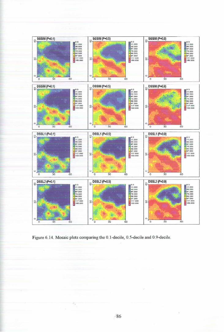
~0.0
'41 .000 MOOO 6 7.000 7 15.000 81l.OOO 97.000 1 17 000
150.000
0
Figure 6.14. Mosaic plots comparing the 0.1-decile, 0.5-decile and 0 .9-decile.
86
~00
.. 1.000 MOOD 67.000 78.000 SQOOO 97.000 117.000
150.000
~0 0
4 1 .000 56.000 07.000 70.000 ggooo 0 7 .000 1 17 000
160.000
~00
-11 .000 MOOO 67 .000 715 .000 sgooo 97 .000 1 •17 000
150.000
~0.0
41 .000 66.000 e r.ooo 7 C5.000 8 9.000 0 7.000 117 000
150.000

The 0.1, 0.5 and 0.9 deciles are displayed for each algorithm. There appears
to be a greater spread in the region of low values for SGSIM and DSSIM. All the
algorithms have a similar distribution in the southwest. In the southeast ther are
more high values for SGSIM and DSSIM. The red areas in the 0.1-quantile plots
indicate that there is a high possiblity that the unknown permeability values in this
region are high, since these values are exceeded by ninety percent of the simulated
values. SGSIM and DSSIM have a similar uncertainty associated with there spatial
distributions as do DSSL1 and DSSL2.
Two grid nodes were selected from regions displaying different spatial uncertainty
to compare the parametric and non-parametric algorithms. T he true potassium
values at locations u 1 = (28.5, 44.5) and u 2 = (28.5, 22.5) are 57.975 and 202.381
respectively and these are represented by the dashed lines in Figure 6.15.
Conditional CDF Models at Ur(28.5,44.5) Conditional CDF Models at Ur(28.5,22.5)
0.8 0.8
~ 0.6 :s "' Q 0 ... 0.4 - SGSIM Q.
~ 0.6 :a "' Q 0 0.4 g: - SGSIM
- DSSIM - OSSIM - DSSL1
0.2 - DSSL2 0.2 - OSSL1
OSSL2
0 0
0 20 40 60 60 100 0 60 120 180 240 300 360
Potassium Pot11ssium
Figure 6.15. Local conditional cumulative distributions.
At location u 1 the cumulative histograms for DSSL1 and DSSL2 are almost
identical, and very steep, indicating the value is likely to be less than 40. This
is considerably less than the true value of 57.975, but all the algorithms include
the true value in their range of potassium values. These differ markedly from the
SGSIM and DSSIM cmnulative histograms. The DSSIM algorithm has the highest
probability of attaining the true value at this location.
At location u 1 the cumulative histograms are different for all a lgorithms, al
though SGSIM and DSSIM are almost identical for the lower fifty percent of values.
87

SGSIM only has a very small probability of attaining the true potassium value, less
than five percent. The DSSIM algorithm does not include the true value of 202.381
in its range of potassium values. The greatest probability of the true potassium value
being attained, approximately twenty five percent., is with the DSSL2 a lgorithm.
The conditional variance for each algorithm is displayed through mosaic maps
in Figure 6.16. The DSSIM algorithm does not indicate any regions of significantly
high uncertainty. The SGSIM, DSSLl and DSSL2 all indicate some areas where
the uncertainty is very high. This appears to be greatest in the band of high values
where sample data are sparsely located. The greatest uncertainty within the low
valued areas is in the NW corner, but none of ihe algorithms indicate this to be a
significant amount.
0 SGSIM CONDITIONAL VARIANCE
•.0 0 0
(J
•••
0
~000
400ll00 !'I!XI [10('1
R()(l 000 1000 000 t:::oo roo 1oo4fJU OOU
10()tt O:::•ll 1eoo oon ~0000
0 DSSL 1 CONDITIONAL VARIANCE
I.L) 0 0
u 1"11
0
::!00 oco <IDOUUO I)(XJ rJ,"Y.J
eoo nm 1000 000 t::oo ooo 14tJU OOU
1eoo rot• ·~o ron 2000 000
0 DSSIM CONDITIONAL VARIANCE
~ 00
u ,,
0
::!00 000 ·HAl uCo:J
!'l·onoo Rnn noo !COO 000 1:::00 CQC• 1ol00 cuu \OUtl O:llo
100CI o:•n :::oooooo
o DSSL2 CONDITIONAL VARIANCE ~ 00
u fT1
0
0 30 60
.;:ooo ... o 41;10.) uoo nonoo
zooo 000
Figure 6.16. Comparison of conditional variance for the algorithms.
88

6. 7 Summary for Potassium
These results for Potas8ium have coniirmed what we already knew about the SGSIM
algorithm. This algorithm has very good reproduction of the semivariogram model
when using normal score data and it reproduces the sample distribution since these
were the values used to produce the normal score data. The DSSIM algorithm did
not reproduce the target semivariogram very well in either the direction of maxi
mum continuity, N65W, or the minor direction, N25E. DSSIM reproduces the local
conditional distribution that was used, in this case a Gaussian distribution. With
the exception of the lower tail which is affected by the inability of the algorithm to
converge and find a feasible solution, the DSSLl and DSSL2 both reproduced the
global distribution very well. There is very little difference between the results of the
DSSLl and DSSL2 algorithms. The DSSLl and DSSL2 algorithms both had trou
ble reproducing the model semivariograrn for a large number of realisations. Both
algorithms have some very extreme semivariograrns1 but for those that do show a
reasonable reproduction, DSSL2 appears to have a larger proportion of experimental
semivariograms closer to the target. For this anisotropic model, the DSSL2 algo
rithm would therefore appear to provide the best reproduction of both the histogram
and the semivariogram.
89

7 Results and Conclusions
In this study we investigated four sequential simulation algorithms, namely se
quential Gaussian simulation (SGSIM), the original direct sequential simulation
(DSSIM), and two direct sequential simulation with histogram reproduction algo
rithms, one using the one-norm (DSSLl) and the other the twe>-norm (DSSL2). We
were interested to see how the algorithms with histogram reproduction compared to
each other and to the more traditional SGSIM and DSSIM algorithms.
This study used two data sets displaying different characteristics. The permeabil
ity data display a strong positive skewness and are from a 2-D section of a reservoir.
The potassium data exhibit a slight positive skewness and the values come from
soil samples. Both data sets comprise a sample data set and an exhaustive data set
which establishes a target distribution and a reference for comparing the different
simulation algorithms.
An important aim of this study was to determine if it is possible for a simulation
algorithm to reproduce both the histogram and the experimerl .. W semivariogram
model without the need for a normal score tra.nsforrnation. Secondly, we wanted to
compare two alg;orithms, one based on the one-norm and the other on the two-norm,
to see if the natural measure produced better r,~sults. Thirdly, we were interested
in the computational effort required for both algorithms.
Each simulation algorithm generated 100 realisations and the simulation results
are produced in both tabloid and graphical form. The histograms and experimental
semivariograms for each realisation were compared to the exhaustive data sets. Two
measures of accuracy were used in analysing the histogram reproduction. This was
done hecause the mean absolute deviation is related to the DSSLl algorithm and
the mean squared deviation is related to the DSSL2 algorithm. By using both mea
surements in the comparisons, a preference is not being unduly given to a particular
algorithm. For the experimental semivariograms, the mean squared deviation from
the target semivariogram model was computed.
The realisations were ranked according to their increasing deviation from the
target •1alues and the minimum, median and maximum realisations from each algo
rithm were used in the comparison of results. The multiple realisations generated
90

help depict the uncertainty about the spatial distribution of the data. The results
were analysed graphically through the use of histograms, cumulative distribution
functions, mosaic maps and semivariograrns and with tables using the accuracy
measurements. These results were compared between individual realisations and
between the different algorithms.
Histogram reproduction without the need for a transformation into normal space
or the rnultiMGaussian assumptions was found to be possible using either the DSSLl
or DSSL2 algorithms, although we will discuss later in this chapter some problems
that were encountered with these two simulation algorithms. The DSSIM algorithm
reproduced the local conditional distribution and not the target distribution, and
SGSIM reproduced d~e sample distribution and not the target distribution. These
two algorithms would require a transformation in order to reproduce the required
target distribution.
Semi variogram reproduction was best when SGSIM was used, but this was in
normal score space. The normal score data must be backMtransfonned and the excelM
lent variogram reproduction may then destroyed (Caers, 2000b). DSSIM was unable
to reproduce the model experimental sernivariogram. The experimental semivariM
ograms calculated for the DSSIM realisations were not at all representative of the
experimental semivariogram model. Both the DSSLI and DSSL2 algorithms were
able to reproduce the experimental semivariogram model. This was better with the
omnidirectional Permeability data set than with the anisotropic Potassium data set.
The results for the DSSL! and DSSL2 algorithms are very similar.
Mosaic maps displaying the 0.1, 0.5 and 0.9 deciles were generated for each
simuh1tion algorithm, along with conditional variance maps. These display the un
certainty in a distribution and may influence the choice of algorithm used. These
characteristics are also very similar with the DSSLI and DSSL2 algorithms, but the
DSSL2 has a slightly higher variation in its higher valued areas than DSSLl.
The DSSLI and DSSL2 algorithms both encountered situations when a feasible
solution could not Le found to the objective function and a decision was made to set
the random deviate equal to the simple kriging mean when this occurred. Figure
7.1 compares the number of infeasible solutions encountered by both algorithms for
the data sets.
91

Infeasible Solutions for Permeability Data. Infeasible Solutions for Potassium Data.
100
80
~ = IU
60
= 17 40 IU
Lt 20
- DSSL1
- DSSL2
300 600 900 1200 1500 1800 0
0 200 400 600 800 1000
II Infeasible Solutions II Infeasible Solutions
Figure 7.1. Comparison of infeasible solutions encountered for Permeability (left) and
Potassium (right) .
fu Table 7.1 we see that the average percentage of solutions that did not converge
was significantly high, especially for the potassium data set. fu both cases DSSL2
had fewer infeasible solutions occUlTing but the number is still very high. This
appears to have had an impact on the number of low values within a realisation.
The number of very low values may be artificially high and improving this situation
should result in better histogram and variogram reproduction.
Table 7.1. Perecentage of infeasible solutions encountered by DSSLl and DSSL2.
Percentage of Infeasible Solutions DSSL1 DSSL2
Permeability 10.3 9.1
Potassium 17.7 16.3
Fmther research is needed to find a way to overcome this problem. Adding local
accmacy to the simulation ( Caers, 2000a) by adding a spike in the local condi
tional distribution increases the connectivity of extreme values and may be a way to
improve the histogram reproduction and reduce the number of infeasible solutions
encountered by the algorithm. It is likely this will affect the variogram reproduction
and a compromise may have to be found.
The global distribution used in this analysis was taken to be the exhaustive data
set. When the sample data are not truly representative of the distribution, it may
help to use a smoothed distribution based on the exhaustive data set to create the
threshold values Tequired for the DSSLl and DSSL2 algorithms.
92

Another factor to take into account when deciding which of the two algoritlnns
is better, is the time taken to execute the simulations. This time factor was very
noticeable in our study. The time will vary depending on the specifications of the
computer system, but we found on average that the DSSL2 algorithm takes approx
imately 3.5 times as long as the DSSLl algorithm for the Permeability data set and
almost 6 times as long for the Potassiwn data set, as seen in Table 7 .2.
Table 7.2. Computation time for DSSLl and DSSL2.
Computation Time per Simulation DSSLl DSSL2
Permeability 24 82
Potassium 6 35
We believe that 'improvements in the current programming structure will de
crease this slightly, but the DSSL2 will still take longer than the DSSLl algorithm.
These simulation methods arc both considerably slower than sequential Gaussian
simulation and direct sequential simulation which give ahnost instantaneous results,
so when one of those methods is suitable to the analysis required, it is recommended
that it be used.
In sununary, this analysis has shown that it is possible to reproduce both the
histogram {cmnulative distribution function) and the semivariogram ru.ing direct
sequential simulation and without the need for a transformation into nonnal space
or the assumption of nonnality. This was found to be possible using a choice of
objective functions based on either the one-norm or the two-norm. The decision as
to which algoritlun to use may be influenced by the computational time involved
and the characteristics of the data. The DSSLl algorithm provided the better re
sults for the isotropic Gata set and the DSSL2 algorithm perfonned better with the
anisotropic data set,.
93

8 References
Armstrong, M. (1998). Basic Linear Geostatistics. Berlin: Springer-Verlag.
Barrodale, I. & Roberts, F.D.K. {1978). An efficient algorithm for discrete £1linear
approximation with linear constraints. SIAM J. Num. Anal., 15(3), 603-611.
Barrodale, I. & Roberts, F.D.K. {1980). Algorithm 552. Solution of the con
strained f.1 linear approximation problem. ACM Transactions on Mathematical
Software, 6{2), 231-235.
Bloom, L.M. & Kentwell, D.J. {1999). A geostatistical analysis of cropped and un
cropped soil in the Jimperding Brook catchment area of Western Australia. In
J. Gomez-Hernandez et al (Eds.), ge<JENVII- Geostatistics for environmental
applications (pp. 369-380). Dordrecht: Kluwer Academic Publishers.
Caers, J. (2000a). Adding Local Accuracy to Direct Sequential Simulation. Math
ematical Geology, 32(7), 815-850.
Caers, J. (200Gb). Direct sequential indicator simulation. In Kleingeld, W. & Krige,
D. {Eels.), Geostats 2000: Gape Town, Proceedings of the 6th International
Geostatistics Congress (pp. 39-48), Cape Town, South Africa, April 10-14,
2000.
Chiles, J-P. & Delfiner, P. {1999). Geostatistics: Modelling Spatial Uncertainty.
New York: Wiley-Interscience.
Deutsch, C.V. & Journel, A.G. {1998). GSLIB: Geostatistical Software Library and
User's Guide. Second Edition. New York: Oxford University Press.
Gill, P.E., Murray, W. & Wright, M.H. (1984). Practical Optimisation. London:
Academic Press.
Gill, P.E., Hammarling, S.J., Murray, W., Saunders, M.A. and Wright, M.H.
{1986). User's guide for LSSOL (Version 1.0}: a Fortran package for con
strained linear least-squares and convex quadratic program!f!ing, Report SOL
84-6, Department of Operations Research, Stanford University, California.
94

..•
Goovaerts, P. (1997). Geostatistics for Natural Resources EvaluaUon. New York:
Oxford University Press.
Goovaerts, P. (2001). Geostatistical assessment of the spaces of local1 spatial and
response uncertainty for continuous petrophysical properties. Unpublished pa
per, University of Michigan, Ann Arbor.
Hillier, F.S. & Lieberman, G.J. (1995). Introduction to Operations Research. (6'"'
ed.). New York: McGraw-Hill, Inc.
Journel, A. G. (1994). Modelling Uncertainty: Some conceptual thoughts. In R.
Dimitrakopoulos (Ed.), Geostotistics for the Next Centv.ry, (pp. 30-43). Dor
drecht: Kluwer Academic.
Journel, A. G. & Huijbregts, C.J. {1978). Mining Geostatistics. New York: Acad
emic Press.
Luenberger, D.G. (1989). Linear and Nonlinear Programming. (2nd ed.) Menlo
Park, California: Addison-Wesley.
Remy, N., Shtuka, A., Levy, B. & Caers, J. (2001). GsTL: the Geostatistical Tem
plate Library in C++. Unpublished paper, Stanford University, California.
Serway, R.A. & Beichner, R.J. (2000). Physics for Scientists and Engineers. (5''
ed.). Fort Worth: Saunders College Publishing.
Wackernagel, H. (1995). Multivariate Geostatistics. Berlin: Springer.
Walpole, R.E. & Myers, R.H. {1993). Probability and Statistics for Engineers and
Scientists. (5'h ed.). New York: Macmillan.
Wismer, D.A. & Chattergy, R. {1978). Introduction to Nonlinear Optimization. A
Problem Solving Approach. New York: Elsevier North-Holland, Inc.
Xu, W. & Joumel, A. G. (1994). DSSIM: A general sequential simulation algorithm.
In Report 7, Stanford Center for Reservoir Forecasting, Stanford, CA .
. ,., .. , .. _
95

9 Appendices
APPENDIX A.
Parameter files for Isotropic Case
A1. sgsim.par 97
A2. dssim.par 98
A3. dssll.par 99
A4. dssl2.par 100
AS. target distribution thresholds 101
..... -96

. ~ .
Al sgsim.par
Parameters for SGSIM ********************
START OF PARAMETERS: perrn50.dat 1 2 0 3 -1.0 1 sgsim. trn 0 ref .dat 3 0
0 0 1. Oe21
1.0 2 4
2500.0 2.5 2.0
0 sgsim.dbg sgsim.dat 100 102 102 1 69069 4 12 1 1 0 60.0 o.o
0 no.dat 4
1.0 1.0
0.0
20
3
60.0 0.0
0.0
0.14
1.0 1.0
1.0
1.0 0.0
1.0
1 1 0.86 90.0
24.0 0. 0 o. 0
24.0 o.o
• • •
-file with data columns for X,Y,Z,vr,wt,sec.var. trimming limits
-transform the data (O=no, l=yes) file for output trans table consider ref. dist (O=no, l=yes) file with ref. dist distribution columns for vr and wt zmin,zmax(tail extrapolation) lower tail option, parameter upper tail option, parameter
-debugging level: 0,1,2,3 -file for debugging output -file for simulation output -number of realizations to generate -nx,xmn,xsiz -ny,ymn,ysiz -nz,zmn,zsiz -random number seed -min and max original data for sim -number of simulated nodes to use -assign data to nodes (O=no, l=yes) -multiple grid search (O=no, l=yes),num -maximum data per octant (O=not used) -maximum search radii (hmax,hmin,vert) -angles for search ellipsoid -ktype: O=SK,1=0K,2=LVM,3=EXDR,4=COLC
file with LVM, EXDR, o:r: COLC variable column for secondary variable
-nst, nugget effect -it,cc,ang1,ang2,ang3 -a_hmax, a_hmin, a_vert
······
97

A2 dssim.par
Parameters for DSSIM ********************
START OF PARAMETERS: perm50.dat 120300 -1.0 l.Oe21 0 dssim.trn 0 histsmth.out 1 2 1.0 1 4 0
2500.0 1.0 2.0
dssim.dbg dssim.dat 100 102 1.0 102 1.0 1 0.0 69069 4 20 12 1 1 3 0 60.0 60.0
0. 0 0. 0
1.0 1.0
1.0
0.0 0. 0 1.0 0 0.60
592.53 582.95 2 nodata.dat 4 2 1
43680 0.0
0.0 1
63000 90.0 0.0 10.0 10.0
124000 90.0 o.o o.o 50.0 50.0
0.0
-file with data -columns for X,Y,Z,vr,wt,sec.var. -trimming limits -transform the data (O=no, l=yes) -file for o~tput trans table -consider ref, dist {O=no, l=yes) -file with ref. dist distribution -columns for vr and wt -zmin, zmax {tail extrapolatio;::.) -lower tail option, parameter -upper tail option, parameter -debugging level: 0,1,2,3 -file for debugging output -file for simulation output -number of realizations to generate -nx,xmn,xsiz -ny,ymn,ysiz -nz,zmn,zsiz -random number seed -min and max original data for sim -number of simulated nodes to use -assign data to nodes {O=no, 1=yes) -multiple grid search {O=no, 1~es) ,num -maximum data per octant (O=not used) -maximum search radii {hmax,hmin,vert) -angles for search ellipsoid -ktyp~: O=SK,l=OK,2=LVM,3=EXDR,4=COLC -global mean, standard deviation - local dist:1-normal,2-lognormal
file with LVM, EXDR, or COLC variable column for secondary variable
-nst, nugget effect -it,cc,ang1,ang2,ang3 -a_hmax, a_hmin, a_vert -it,cc,angl,ang2,ang3 -a_hmax, a_hmin, a_vert
98

A3 dssll.par
Parameters for DSSLl ********************
START OF PARAMETERS: permS 0. da t 120300 -1.0 0
l.Oe21
dssLl. trn 0 histsmth.out 1 2 p40.dat dssll.inf 2 1
1.0 2500.0 1 1.0 1 2500.0 1 dssLl.dbg dssLl.dat 100 102 102 1 69069 4 12 1
1.0 1.0
0.0
20
1 3 0 60.0 60.0
0. 0 0. 0 0 0.60 592.53 nodata.dat 4
43680
1.0 1.0
1.0
1.0 0.0 1.0
582,95
2 1
1
63000 90.0 o.o 0.0 10.0 10.0 0.0
124000 90.0 0.0 0.0 50.0 50.0 0.0
-file with data -columns for X,Y,Z,vr,wt,sec.var. -trimming limits -transform the data (O=no, l=yes) -file for output trans table -consider ref. dist (O=no, l=yes) -file with ref. dist distribution -columns for vr and wt -cdf file -info file -select(l-DSSIM,2-DSSL1)opt(l-skmean,
2-logsim,3-normal) -zmin,zmax(tail extrapolation) -lower tail option, parameter -upper tail option, parameter -debugging level: 0,1,2,3 -file for debugging output -file for simulation output -number of realizatiuns to generate -nx,xmn,xsiz -ny,ymn,ysiz -nz,zrnn,zsiz -random number seed -min and max original data for sim -number of simulated nodes to use -assign data to nodes (O=no, l=yes) -multiple grid search (O=no, l=yes),num -maximum data per octant {O=not used) -maximum search radii (lunax,hJ.•in,vert) -angles for search ellipsoid -ktype: O=SK,l=OK,2=LVM,3=EXDR,4=COLC -global mean, standard deviation -file with LVM, EXDR, or COLC variable -column for secondary variable -nst, nugget effect -it,cc,angl,ang2,ang3 -a_hmax, a_hmin, a_vert -it,cc,angl,ang2,ang3 -a_hmax, a_hmin, a_vert
99

A4 dssl2.par
Parameters for DSSL2 ********************
START OF PARAMETERS: permSO,dat 1 2 0 3 -1.0 0 dssL2. trn 0
0 0 l.Oe21
histsmth.out 1 2 p40.dat dssL2. in£ 210 1.0 1 1 1
2500.0 1.0
2500.0
dssL2 .dbg dssL2 .dat 100 102 1. 0 102 1. 0 1 0. 0 69069 4 20 12 1 1 3 0 60.0 60.0 o. 0 0. 0
0 0. 60 592.53 nodata,dat 4
43680
1.0 1.0
1.0
1.0 o.o 1.0
582.95
2 1
1
63000 90.0 0.0 10.0 10.0
124000 90.0 0.0 50.0 50.0
o.o 0.0
0.0 o.o
-file with data columns for X,Y,Z,vr,wt,sec.var. trimming limits
-transform the data (O=no, l=yes) -file for output trans table -consider ref. dist (O=no, l=yes) -file with ref. dist distribution -columns for vr and wt -cdf file -output info file -select l-DSSIM,2-DSSL2 opt: l-QP2,2-LS1 -zmin,zmax(tail extrapolation) -lower tail option, parameter -upper tail option, parameter -debugging level: 0,1,2,3 -file for debugging output -file for simulation output -number of realizations to generate -nx,xmn,xsiz -ny,ymn,ysiz -nz,zmn,zsiz -random number seed -min and max original data for sim -number of simulated nodes to use -assign data to nodes (O=no, l=yesl -multiple grid search (O=no, l=yes),num -maximum data per octant (O=not used) -maximum search radii (hmax,hmin,vert) -angles for search ellipsoid -ktype: O=SK,l=OK,2=LVM,3=EXDR,4=COLC -global mean, standard deviation -file with LVM, EXDR, or COLC variable -cOlumn for secondary variable -nst, nugget effect -it,cc,angl,ang2,ang3 -~hmax, a_hmin, a_vert -it,cc,angl,ang2,ang3 -a_bmax, a_hmin, a_vert
100

AS p40.dat
p40 3 40 i k prob 1 17. 5869775 0.025 2 43.547355 0.025 3 80.4025825 0.025 4 117.25781 0.025 5 146' 372725 0.025 6 163.18037 0. 025 7 179.987915 0. 025 8 191.95234 0.025 9 193.0798025 0.025 10 194.207325 0,025 11 195.5754475 0.025 12 197.74167 0. 025 13 199.9079925 0.025 14 205.601605 0.025 15 230.6076125 0. 025 16 255.61362 0.025 17 283.75861 0. 025 18 349.414575 0. 025 19 415.07057 0. 025 20 480.6922 0. 025 21 510.626525 0.025 22 540.52645 0. 025 23 570.426375 0. 025 24 595.14352 0.025 25 619.426925 0. 025 26 643.71033 0.025 27 706.7461425 0.025 28 776.85997 0.025 29 846.973945 0.025 30 869.159725 0. 025 31 876.8952525 0.025 32 884.63078 0.025 33 974.5320775 0.025 34 1101.154505 0.025 35 1227.776875 0.025 36 1340.76718 0.025 37 1445.18373 0,025 38 1549.600405 0.025 39 1912.615898 0.025 40 2498.8733 0.025
101

APPENDIX B.
Parameter files for Anisotropic Case
B!. sgsim.par 103
82. dssim.par 104
83. dssll.par !OS
84. dssl2.par 106
85. target distribution thresholds 107
102

Bl sgsim.par
Parameters for SGSIM ******************••
START OF PARAMETERS: klOO.dat 120300 -1. 0 1. Oe21 1 sgsim, trn 0 histsmth.out 1 2 20.0 1
360.0 20.0
4 1.5 1 sgsim.dbg sgsim.dat 100 60 0.5 60 0.5 1 0.0 69069 < 20 12 1 1 3 0 40.0 40.0
0. 0 0.0 0 0. 0 87.097 nodata.dat 4 1 0. 08
1.0 1.0 1.0
1.0 0.0
1.0 34.703
1 0.92 115.0 25.0 16.0
0.0 0.0
0,0
-file with data columns for X,Y,Z,vr,wt,sec.var. trimming limits
-transform the data (O=no, l=yes) -file for output trans table -consider ref. dist (O=no, l=yes) -file with ref. dist distribution -columns for vr and wt -zmin,zmax(tail extrapolation) -lower tail option, parameter -upper tail option, parameter -debugging level: 0,1,2.3 -file for debugging output -file for simulation output -number of realizations to generate -nx,xmn,xsiz -ny,ynm,ysiz -nz,znm,zsiz -random number seed -min and max original data for sim -number of simulated nodes to use -assign data to nodes (O=no, l=yes) -multiple grid search {O=no, l=yes),num -maximum data per octant (O=not used) -maximum search radii (lunax,hmin,vert) -angles for search ellipsoid -ktype: O~SK,l=OK,2=LVM,3=EXDR,4=COLC
-global mean, standard deviation -file with LVM, EXDR, or COLC variable -column for secoadary variable -nst, nugget effect -it,cc,angl,ang2,ang3 -a_hmax, a_hmin, a_vert
103

B2 dssim.par
Parameters for DSSIM
***** ****** *** *** ***
START OF klOO.dat 1 2 0 -1.0
PARAMETERS:
3 0 0 l.Oe21
0 direct_k. trn 0 histsmth.out 1 2 20,0 1 4 0
360,0 20.0 1.5
direct_k.dbg direct_k.dat 100 60 0 .s 60 0.5 1 0.0 69069 4 20 12 1 1 3 0 40.0 40.0
0. 0 o.o 0 0.60
1.0 1.0 1.0
0.0 0.0 1.0
89.45 34.42 nodata.dat 4 1 1
84 1104 115.0 0.0 o.o
22.0 16.72 0.0
-file with data columns for X,Y,Z,vr,wt,sec.var. trinuning limits
-transform the data {O=no, l=yes) file for output trans table consider ref. dist (O=no, l=yes) file with ref. dist distribution columns for vr and wt zmin, zmax {tail extrapolation) lower tail option, parameter upper tail option, parameter
-debugging level: 0,1,2,3 -file for debugging output -file for simulation output -number of realizations to generate -nx,xmn,xsiz -ny ,ymn,ysiz -nz, zrnn, zsiz -random number seed -min and max original data for sim -number of simulated nodes to use -assign data to nodes {O=no, l=yes) -multiple grid search {O=no, !=yes) ,num -maximum data per octant {O=not used) -maximum search radii {hma:x,hmin,vert) -angles for search ellipsoid -ktYPe: O=SK, l=Olt, 2=LVM, 3=EXDR, 4=COLC -global mean, standard deviation
file with LVM, EXDR, or COLC variable column for secondaiy variable
-nst, nugget effect -it,cc,angl,ang2,ang3 -a-Pmax, a_hmin, a_vert
104

B3 dssll.par
Parameters for DSSLl ********************
START OF PARAMETERS: klOO.dat 120300 -1.0 l.Oe21 0 dssim. trn 0 histsrnth.·.:mt 1 2 k40.dat dssim.inf 2 1
20.0 360.0 1 20.0 1 360.0 1 dssim.dbg dssim.dat 100 60 0.5 1.0 60 0.5 1.0 1 0. 0 1.0 69069 4 20 12 1 1 3 0 40.0 40.0 1.0
0.0 0.0 0.0 0 0.60 1.0 89.45 34.42 nodata.dat 4 1 84 1 1104 115.0 0.0 0.0
22.0 16.72 0.0
-file with data -columns for X,Y,Z,vr,wt,sec.var. -trimming limits -transform the data (O~no, l=yes) -file for output trans table -consider ref. dist (O=no, l=yes) -file with ref. dist distributi-on -columns for vr and wt -cdf file -info file -select(l-DSSIM,2-DSSLl)opt(1-skmean,
2-logsim, 3 -normal) -zmin,zmax(tail extrapolation) -lower tail option, parameter -upper tail option, parameter -debugging level: 0,1,2,3 -file for debugging output -file for simulation output -number of realizations to generate -nx,xrnn,xsiz -ny,ymn,ysiz -nz,zmn,zsiz -random number seed -min and max original data fo.r sim -number of simulated nodes to use -assign data to nodes (O=no, l=yes) -multiple grid search (O=no, l=yes),num -maximum data per octant (O=not used) -maximum search radii (hmax,hmin,vert} -angles for search ellipsoid -ktype: O=SK,l=OK,2=LVM,3=EXDR,4=COLC -global mean, standard deviation
file with LVM, EXDR, or COLC variable column for secondary variable
-nst, nugget effect -it,cc,angl,ang2,ang3 -a_hmax, a_hmin, a_vert
105

B4 dssl2.par
Parameters for DSSL2 ********************
START OF PARAMETERS: klOO ,dat 120300 -1.0 l.Oe21 0 dSSL2. trn 0 histsmth.out 1 2 k40. dat dssL2.inf 2 10 20.0 1 1 1
360.0 20.0 360.0
dssL2.dbg dSSL2.dat 100 60 0.5 60 0,5 1 0.0 69069 4 20 12 1 1 3
1.0 1.0 1.0
0 40.0
0. 0 0 89.45
40.0 1.0 0. 0 0. 0
0,60 1.0 34.42
nodata.dat 4 1 1
84 1104 115.0 0.0
22.0 16.72 0.0 0.0
-file with data columns for X,Y,Z,vr,wt,sec.var. trimming limits
-transform the data (O=no, l=yes) -file for output trans table -consider ref. dist {O=no, l=yes) -file with ref. dist distribution -columns for vr and wt -cdf file -output info file -select l-dssim,2-dssl2 opt:10-QP2,20-LS1 -zmin,zmax(tail extrapolation) -lower tail option, parameter -upper tail option, parameter -debugging level: 0,1,2,3 -file for debugging output -file for simulation output -number of realizations to generate -nx,xmn,xsiz -ny,ymn,ysiz -nz,zmn,zsiz -random number seed -min and max original data for sim -number of simulated nodes to use -assign data to nodes (O=no, l=yes) -multiple grid search (O=no, 1=yes),num -maximum data per octant (O=not used) -maximum search radii (hnmx,hmin,vert) -angles for search ellipsoid -ktype: O=SK, 1=0K, 2=LVM, 3=EXDR, 4=COLC -global mean, standard deviation -file with LVM, EXDR, or COLC variable -column for secondary variable -nst, nugget effect -it,cc,angl,ang2,ang3 -a_hnmx, a_hmin, a_vert
106

BS k40.dat
k40 3 40 i k prob 1 38.15775 0.025 2 41.8968 0,025 3 45.1628 0.025 4 48 0.025 5 49.57725 0.025 6 51.78715 0.025 ? 53.9086 0.025 8 55.872 0.025 9 57.79575 0.025 10 59.85275 0,025 11 62.525 0. 025 12 64.7698 0. 025 13 67.0457 0. 025 14 69.2315 o. 025 15 71.778 0. 025 16 73. 6688 0. 025 17 76.21795 0. 025 18 78.12165 0.025 19 80.387 0.025 20 82.326 0.025 21 84.85635 0.025 22 87.22815 0.025 23 89.323 0.025 24 91.367 0,025 25 93.94825 0.025 26 96.38045 0.025 2? 98.5661 0.025 28 101.1474 0.025 29 104.115 0. 025 30 106.8665 0.025 31 109.6984 0.025 32 112. 9QB 0.025 33 117.162 0.025 34 121.31225 0.025 35 125.7195 0.025 36 130.7551 0,025 37 139.59615 0.025 38 150.5525 0.025 39 168.418 0.025 40 331.978 0.025
107


![Sequential unconstrained minimization algorithms for constrained …faculty.uml.edu/cbyrne/summa2.pdf · 2008. 1. 10. · sequential unconstrained minimization algorithms [15]. We](https://img.pdfslide.us/doc/110x75/611fc7373f6d994a6c4a2ffa/sequential-unconstrained-minimization-algorithms-for-constrained-2008-1-10.jpg)