Direct Prediction of 3D Body Poses from Motion Compensated Sequences

Bugra Tekin1 Artem Rozantsev1 Vincent Lepetit1,2 Pascal Fua1

1CVLab, EPFL, Lausanne, Switzerland, firstname.lastname@epfl.ch2TU Graz, Graz, Austria, lepetit@icg.tugraz.at

Abstract

We propose an efficient approach to exploiting motion

information from consecutive frames of a video sequence to

recover the 3D pose of people. Previous approaches typ-

ically compute candidate poses in individual frames and

then link them in a post-processing step to resolve ambigui-

ties. By contrast, we directly regress from a spatio-temporal

volume of bounding boxes to a 3D pose in the central frame.

We further show that, for this approach to achieve its

full potential, it is essential to compensate for the motion

in consecutive frames so that the subject remains centered.

This then allows us to effectively overcome ambiguities and

improve upon the state-of-the-art by a large margin on the

Human3.6m, HumanEva, and KTH Multiview Football 3D

human pose estimation benchmarks.

1. Introduction

In recent years, impressive motion capture results have

been demonstrated using depth cameras, but 3D body pose

recovery from ordinary monocular video sequences remains

extremely challenging. Nevertheless, there is great inter-

est in doing so, both because cameras are becoming ever

cheaper and more prevalent and because there are many po-

tential applications. These include athletic training, surveil-

lance, and entertainment.

Early approaches to monocular 3D pose tracking in-

volved recursive frame-to-frame tracking and were found to

be brittle, due to distractions and occlusions from other peo-

ple or objects in the scene [43]. Since then, the focus has

shifted to “tracking by detection,” which involves detect-

ing human pose more or less independently in every frame

followed by linking the poses across the frames [2, 31],

which is much more robust to algorithmic failures in iso-

lated frames. More recently, an effective single-frame ap-

proach to learning a regressor from a kernel embedding

of 2D HOG features to 3D poses has been proposed [17].

Excellent results have also been reported using a Convolu-

tional Neural Net [25].

However, inherent ambiguities of the projection from 3D

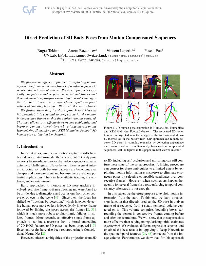
Figure 1. 3D human pose estimation in Human3.6m, HumanEva

and KTH Multiview Football datasets. The recovered 3D skele-

tons are reprojected into the images in the top row and shown

by themselves in the bottom row. Our approach can reliably re-

cover 3D poses in complex scenarios by collecting appearance

and motion evidence simultaneously from motion compensated

sequences. All the figures in this paper are best viewed in color.

to 2D, including self-occlusion and mirroring, can still con-

fuse these state-of-the-art approaches. A linking procedure

can correct for these ambiguities to a limited extent by ex-

ploiting motion information a posteriori to eliminate erro-

neous poses by selecting compatible candidates over con-

secutive frames. However, when such errors happen fre-

quently for several frames in a row, enforcing temporal con-

sistency afterwards is not enough.

In this paper, we therefore propose to exploit motion in-

formation from the start. To this end, we learn a regres-

sion function that directly predicts the 3D pose in a given

frame of a sequence from a spatio-temporal volume cen-

tered on it. This volume comprises bounding boxes sur-

rounding the person in consecutive frames coming before

and after the central one. We will show that this approach is

more effective than relying on regularizing initial estimates

a posteriori. We evaluated different regression schemes and

obtained the best results by applying a Deep Network to

the spatiotemporal features [21, 45] extracted from the im-

age volume. Furthermore, we show that, for this approach

991

to perform to its best, it is essential to align the succes-

sive bounding boxes of the spatio-temporal volume so that

the person inside them remains centered. To this end, we

trained two Convolutional Neural Networks to first predict

large body shifts between consecutive frames and then re-

fine them. This approach to motion compensation outper-

forms other more standard ones [28] and improves 3D hu-

man pose estimation accuracy significantly. Fig. 1 depicts

sample results of our approach.

The novel contribution of this paper is therefore a princi-

pled approach to combining appearance and motion cues to

predict 3D body pose in a discriminative manner. Further-

more, we demonstrate that what makes this approach both

practical and effective is the compensation for the body mo-

tion in consecutive frames of the spatiotemporal volume.

We show that the proposed framework improves upon the

state-of-the-art [2, 3, 4, 17, 25] by a large margin on Hu-

man3.6m [17], HumanEva [36], and KTH Multiview Foot-

ball [6] 3D human pose estimation benchmarks.

2. Related Work

Approaches to estimating the 3D human pose can be

classified into two main categories, depending on whether

they rely on still images or image sequences. We briefly

review both kinds below. In the results section, we will

demonstrate that we outperform state-of-the-art representa-

tives of each of these two categories.

3D Human Pose Estimation in Single Images. Early

approaches tended to rely on generative models to search

the state space for a plausible configuration of the skeleton

that would align with the image evidence [12, 13, 27, 35].

These methods remain competitive provided that a good

enough initialization can be supplied. More recent ones [3,

6] extend 2D pictorial structure approaches [10] to the 3D

domain. However, in addition to their high computational

cost, they tend to have difficulty localizing people’s arms

accurately because the corresponding appearance cues are

weak and easily confused with the background [33].

By contrast, discriminative regression-based ap-

proaches [1, 4, 16, 40] build a direct mapping from image

evidence to 3D poses. Discriminative methods have been

shown to be effective, especially if a large training dataset,

such as [17] is available. Within this context, rich features

encoding depth [34] and body part information [16, 25]

have been shown to be effective at increasing the estima-

tion accuracy. However, these methods can still suffer

from ambiguities such as self-occlusion, mirroring and

foreshortening, as they rely on single images. To overcome

these issues, we show how to use not only appearance, but

also motion features for discriminative 3D human pose

estimation purposes.

In another notable study, [4] investigates merging image

features across multiple views. Our method is fundamen-

tally different as we do not rely on multiple cameras. Fur-

thermore, we compensate for apparent motion of the per-

son’s body before collecting appearance and motion infor-

mation from consecutive frames.

3D Human Pose Estimation in Image Sequences.

Such approaches also fall into two main classes.

The first class involves frame-to-frame tracking and dy-

namical models [43] that rely on Markov dependencies on

previous frames. Their main weakness is that they require

initialization and cannot recover from tracking failures.

To address these shortcomings, the second class focuses

on detecting candidate poses in individual frames followed

by linking them across frames in a temporally consistent

manner. For example, in [2], initial pose estimates are re-

fined using 2D tracklet-based estimates. In [47], dense op-

tical flow is used to link articulated shape models in ad-

jacent frames. Non-maxima suppression is then employed

to merge pose estimates across frames in [7]. By contrast

to these approaches, we capture the temporal information

earlier in the process by extracting spatiotemporal features

from image cubes of short sequences and regressing to 3D

poses. Another approach [5] estimates a mapping from

consecutive ground-truth 2D poses to a central 3D pose.

Instead, we do not require any such 2D pose annotations

and directly use as input a sequence of motion-compensated

frames.

While they have long been used for action recogni-

tion [23, 45], person detection [28], and 2D pose estima-

tion [11], spatiotemporal features have been underused for

3D body pose estimation purposes. The only recent ap-

proach we are aware of is that of [46] that involves build-

ing a set of point trajectories corresponding to high joint

responses and matching them to motion capture data. One

drawback of this approach is its very high computational

cost. Also, while the 2D results look promising, no quan-

titative 3D results are provided in the paper and no code is

available for comparison purposes.

3. Method

Our approach involves finding bounding boxes around

people in consecutive frames, compensating for the motion

to form spatiotemporal volumes, and learning a mapping

from these volumes to a 3D pose in their central frame.

In the remainder of this section, we first introduce our

formalism and then describe each individual step, depicted

by Fig. 2.

3.1. Formalism

In this work, we represent 3D body poses in terms of

skeletons, such as those shown in Fig. 1, and the 3D loca-

tions of their D joints relative to that of a root node. As

several authors before us [4, 17], we chose this representa-

tion because it is well adapted to regression and does not

992

(a) Image stack (b) Motion compensation (c) Rectified spatiotemporal volume (d) Spatiotemporal feautures (e) 3D pose regression

Figure 2. Overview of our approach to 3D pose estimation. (a) A person is detected in several consecutive frames. (b) Using a CNN, the

corresponding image windows are shifted so that the subject remains centered. (c) A rectified spatiotemporal volume (RSTV) is formed

by concatenating the aligned windows. (d) A pyramid of 3D HOG features are extracted densely over the volume. (e) The 3D pose in the

central frame is obtained by regression.

require us to know a priori the exact body proportions of

our subjects. It suffers from not being orientation invariant

but using temporal information provides enough evidence

to overcome this difficulty.

Let Ii be the i-th image of a sequence containing a sub-

ject and Yi ∈ R3·D be a vector that encodes the corre-

sponding 3D joint locations. Typically, regression-based

discriminative approaches to inferring Yi involve learning a

parametric [1, 18] or non-parametric [42] model of the map-

ping function, Xi → Yi ≈ f(Xi) over training examples,

where Xi = Ω(Ii;mi) is a feature vector computed over

the bounding box or the foreground mask, mi, of the per-

son in Ii. The model parameters are usually learned from

a labeled set of N training examples, T = (Xi,Yi)Ni=1.

As discussed in Section 2, in such a setting, reliably esti-

mating the 3D pose is hard to do due to the inherent ambi-

guities of 3D human pose estimation such as self-occlusion

and mirror ambiguity.

Instead, we model the mapping function f condi-

tioned on a spatiotemporal 3D data volume consisting

of a sequence of T frames centered at image i, Vi =[Ii−T/2+1, . . . , Ii, . . . , Ii+T/2], that is, Zi → Yi ≈ f(Zi)where Zi = ξ(Vi;mi−T/2+1, . . . ,mi, . . . ,mi+T/2) is a

feature vector computed over the data volume, Vi. The

training set, in this case, is T = (Zi,Yi)Ni=1, where Yi is

the pose in the central frame of the image stack. In practice,

we collect every block of consecutive T frames across all

training videos to obtain data volumes. We will show in the

results section that this significantly improves performance

and that the best results are obtained for volumes of T = 24to 48 images, that is 0.5 to 1 second given the 50fps of the

sequences of the Human3.6m [17] dataset.

3.2. Spatiotemporal Features

Our feature vector Z is based on the 3D HOG descrip-

tor [45], which simultaneously encodes appearance and mo-

tion information. It is computed by first subdividing a

data volume such as the one depicted by Fig. 2(c) into

equally-spaced cells. For each one, the histogram of ori-

ented 3D spatio-temporal gradients [21] is then computed.

To increase the descriptive power, we use a multi-scale ap-

proach. We compute several 3D HOG descriptors using dif-

ferent cell sizes. In practice, we use 3 levels in the spatial

dimensions—2×2, 4×4 and 8×8—and we set the temporal

cell size to a small value—4 frames for 50 fps videos—to

capture fine temporal details. Our final feature vector Z is

obtained by concatenating the descriptors at multiple reso-

lutions into a single vector.

An alternative to encoding motion information in this

way would have been to explicitly track body pose in the

spatiotemporal volume, as done in [2]. However, this in-

volves detection of the body pose in individual frames

which is subject to ambiguities caused by the projection

from 3D to 2D as explained in Section 1 and not having

to do this is a contributing factor to the good results we will

show in Section 4.

Another approach for spatiotemporal feature extraction

could be to use 3D CNNs directly operating on the pixel in-

tensities of the spatiotemporal volume. However, in our ex-

periments, we have observed that, 3D CNNs did not achieve

any notable improvement in performance compared to spa-

tial CNNs. This is likely due to the fact that 3D CNNs re-

main stuck in local minima due to the complexity of the

model and the large input dimensionality. This is also ob-

served in [19, 26].

3.3. Motion Compensation with CNNs

For the 3D HOG descriptors introduced above to be rep-

resentative of the person’s pose, the temporal bins must cor-

respond to specific body parts, which implies that the person

should remain centered from frame to frame in the bound-

ing boxes used to build the image volume. We use the De-

formable Part Model detector (DPM) [10] to obtain these

bounding boxes, as it proved to be effective in various ap-

plications. However, in practice, these bounding boxes may

not be well-aligned on the person. Therefore, we need to

993

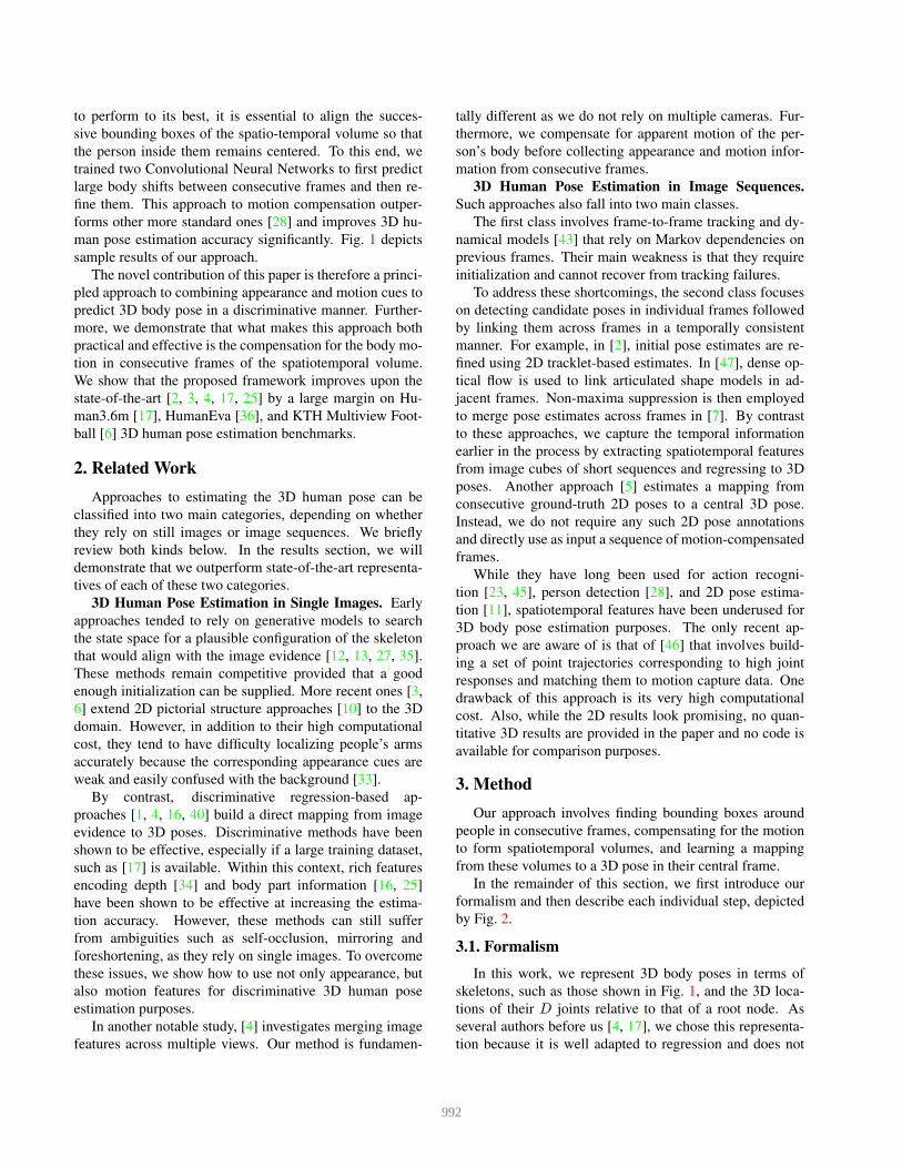
(a) No compensation (b) Motion compensation

Figure 3. Heat maps of the gradients across all frames for Greeting

action (a) without and (b) with motion compensation. When mo-

tion compensation is applied, body parts become covariant with

the 3D HOG cells across frames and thus the extracted spatiotem-

poral features become more part-centric and stable.

first shift these boxes as shown in Fig. 2(c) before creating

a spatiotemporal volume. In Fig. 3, we illustrate this re-

quirement by showing heat maps of the gradients across a

sequence without and with motion compensation. Without

it, the gradients are dispersed across the region of interest,

which reduces feature stability.

We therefore implemented an object-centric motion

compensation scheme inspired by the one proposed in [32]

for drone detection purposes, which was shown to perform

better than optical-flow based alignment [28]. To this end,

we train regressors to estimate the shift of the person from

the center of the bounding box. We apply these shifts to the

frames of the image stack so that the subject remains cen-

tered, and obtain what we call a rectified spatio-temporal

volume (RSTV), as depicted in Fig. 2(c). We have chosen

CNNs as our regressors, as they prove to be effective in var-

ious regression tasks.

More formally, let m be an image patch extracted from a

bounding box returned by DPM. An ideal regressor ψ(·) for

our purpose would return the horizontal and vertical shifts

δu and δv of the person from the center of m: ψ(m) =(δu, δv). In practice, to make the learning task easier, we

introduce two separate regressors ψcoarse(·) and ψfine(·).We train the first one to handle large shifts and the second

to refine them. We use them iteratively as illustrated by

Algorithm 1. After each iteration, we shift the images by

the computed amount and estimate a new shift. This process

typically takes only 4 iterations, 2 using ψcoarse(·) and 2

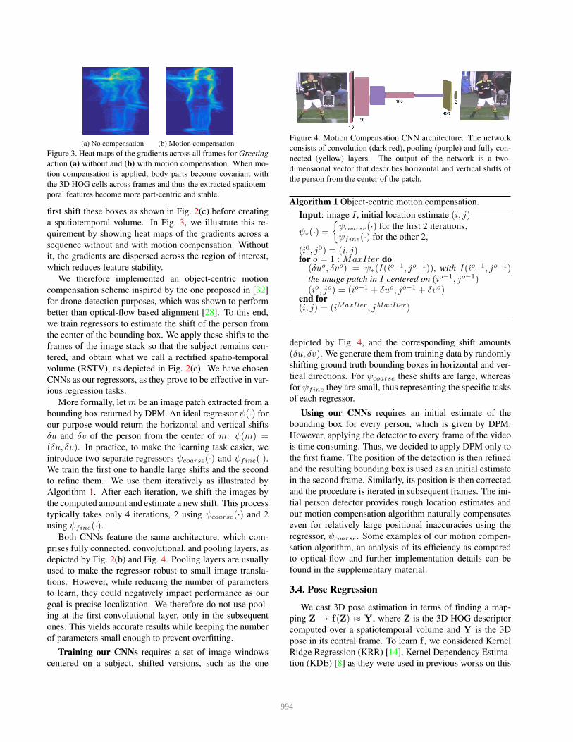
using ψfine(·).Both CNNs feature the same architecture, which com-

prises fully connected, convolutional, and pooling layers, as

depicted by Fig. 2(b) and Fig. 4. Pooling layers are usually

used to make the regressor robust to small image transla-

tions. However, while reducing the number of parameters

to learn, they could negatively impact performance as our

goal is precise localization. We therefore do not use pool-

ing at the first convolutional layer, only in the subsequent

ones. This yields accurate results while keeping the number

of parameters small enough to prevent overfitting.

Training our CNNs requires a set of image windows

centered on a subject, shifted versions, such as the one

Figure 4. Motion Compensation CNN architecture. The network

consists of convolution (dark red), pooling (purple) and fully con-

nected (yellow) layers. The output of the network is a two-

dimensional vector that describes horizontal and vertical shifts of

the person from the center of the patch.

Algorithm 1 Object-centric motion compensation.

Input: image I , initial location estimate (i, j)

ψ∗(·) =

ψcoarse(·) for the first 2 iterations,ψfine(·) for the other 2,

(i0, j0) = (i, j)for o = 1 :MaxIter do(δuo, δvo) = ψ∗(I(i

o−1, jo−1)), with I(io−1, jo−1)the image patch in I centered on (io−1, jo−1)(io, jo) = (io−1 + δuo, jo−1 + δvo)

end for(i, j) = (iMaxIter, jMaxIter)

depicted by Fig. 4, and the corresponding shift amounts

(δu, δv). We generate them from training data by randomly

shifting ground truth bounding boxes in horizontal and ver-

tical directions. For ψcoarse these shifts are large, whereas

for ψfine they are small, thus representing the specific tasks

of each regressor.

Using our CNNs requires an initial estimate of the

bounding box for every person, which is given by DPM.

However, applying the detector to every frame of the video

is time consuming. Thus, we decided to apply DPM only to

the first frame. The position of the detection is then refined

and the resulting bounding box is used as an initial estimate

in the second frame. Similarly, its position is then corrected

and the procedure is iterated in subsequent frames. The ini-

tial person detector provides rough location estimates and

our motion compensation algorithm naturally compensates

even for relatively large positional inaccuracies using the

regressor, ψcoarse. Some examples of our motion compen-

sation algorithm, an analysis of its efficiency as compared

to optical-flow and further implementation details can be

found in the supplementary material.

3.4. Pose Regression

We cast 3D pose estimation in terms of finding a map-

ping Z → f(Z) ≈ Y, where Z is the 3D HOG descriptor

computed over a spatiotemporal volume and Y is the 3D

pose in its central frame. To learn f , we considered Kernel

Ridge Regression (KRR) [14], Kernel Dependency Estima-

tion (KDE) [8] as they were used in previous works on this

994

task [16, 17], and Deep Networks.

Kernel Ridge Regression (KRR) trains a model for

each dimension of the pose vector separately. To find the

mapping from spatiotemporal features to 3D poses, it solves

a regularized least-squares problem of the form,

argminW

∑

i

||Yi −WΦZ(Zi)||22 + ||W||22 , (1)

where (Zj ,Yj) are training pairs and ΦZ is the Fourier

approximation to the exponential-χ2 kernel [17]. This

problem can be solved in closed-form by W =(ΦZ(Z)

TΦZ(Z) + I)−1ΦZ(Z)TY.

Kernel Dependency Estimation (KDE) is a structured

regressor that accounts for correlations in 3D pose space. To

learn the regressor, not only the input as in the case of KRR,

but also the output vectors are lifted into high-dimensional

Hilbert spaces using kernel mappings ΦZ and ΦY , respec-

tively [8, 17]. The dependency between high dimensional

input and output spaces is modeled as a linear function. The

corresponding matrix W is computed by standard kernel

ridge regression,

argminW

∑

i

||ΦY (Yi)−WΦZ(Zi)||22 + ||W||22 , (2)

To produce the final prediction Y, the difference between

the predictions and the mapping of the output in the high

dimensional Hilbert space is minimized by finding

Y = argminY

||WTΦZ(Z)− ΦY (Y)||22 . (3)

Although the problem is non-linear and non-convex,

it can nevertheless be accurately solved given the KRR

predictors for individual outputs to initialize the process.

In practice, we use an input kernel embedding based on

15,000-dimensional random feature maps corresponding to

an exponential-χ2 kernel, a 4000-dimensional output em-

bedding corresponding to radial basis function kernel as

in [24].

Deep Networks (DN) rely on a multilayered architec-

ture to estimate the mapping to 3D poses. We use 3 fully-

connected layers with the rectified linear unit (ReLU) ac-

tivation function in the first 2 layers and a linear activa-

tion function in the last layer. The first two layers con-

sist of 3000 neurons each and the final layer has 51 out-

puts, corresponding to 17 3D joint positions. We performed

cross-validations across the network’s hyperparameters and

choose the ones with the best performance on a validation

set. We minimize the squared difference between the pre-

diction and the ground-truth 3D positions to find the map-

ping f parametrized by Θ:

Θ = argminΘ

∑

i

||fΘ(Zi)−Yi||22 . (4)

We used the ADAM [20] gradient update method to steer

the optimization problem with a learning rate of 0.001 and

dropout regularization to prevent overfitting. We will show

in the results section that our DN-based regressor outper-

forms KRR and KDE [16, 17].

4. Results

We evaluate our approach on the Human3.6m [17],

HumanEva-I/II [36], and KTH Multiview Football II [6]

datasets. Human3.6m is a recently released large-scale mo-

tion capture dataset that comprises 3.6 million images and

corresponding 3D poses within complex motion scenarios.

11 subjects perform 15 different actions under 4 different

viewpoints. In Human3.6m, different people appear in the

training and test data. Furhtermore, the data exhibits large

variations in terms of body shapes, clothing, poses and

viewing angles within and across training/test splits [17].

The HumanEva-I/II datasets provide synchronized images

and motion capture data and are standard benchmarks for

3D human pose estimation. We further provide results on

the KTH Multiview Football II dataset to demonstrate the

performance of our method in a non-studio environment.

In this dataset, the cameraman follows the players as they

move around the pitch. We compare our method against

several state-of-the-art algorithms in these datasets. We

chose them to be representative of different approaches to

3D human pose estimation, as discussed in Section 2. For

those which we do not have access to the code, we used the

published performance numbers and ran our own method

on the corresponding data.

4.1. Evaluation on Human3.6m

To quantitatively evaluate the performance of our ap-

proach, we first used the recently released Human3.6m [17]

dataset. On this dataset, the regression-based method

of [17] performed best at the time and we therefore use

it as a baseline. That method relies on a Fourier approxi-

mation of 2D HOG features using the χ2 comparison met-

ric, and we will refer to it as “eχ2 -HOG+KRR” or “eχ2 -

HOG+KDE”, depending on whether it uses KRR or KDE.

Since then, even better results have been obtained for some

of the actions by using CNNs [25]. We denote it as CNN-

Regression. We refer to our method as “RSTV+KRR”,

“RSTV+KDE” or “RSTV+DN”, depending on whether

we use respectively KRR, KDE, or deep networks on the

features extracted from the Rectified Spatiotemporal Vol-

umes (RSTV). We report pose estimation accuracy in terms

of average Euclidean distance between the ground-truth and

predicted joint positions (in millimeters) as in [17, 25] and

exclude the first and last T/2 frames (0.24 seconds for

T = 24 at 50 fps).

The authors of [25] reported results on subjects S9 and

S11 of Human3.6m and those of [17] made their code avail-

able. To compare our results to both of those baselines, we

therefore trained our regressors and those of [17] for 15 dif-

995

Method Directions Discussion Eating Greeting Phone Talk Posing Buying Sitting

eχ2 -HOG+KRR [17] 140.00 (42.55) 189.36 (94.79) 157.20 (54.88) 167.65 (60.16) 173.72 (60.93) 159.25 (52.47) 214.83 (86.36) 193.81 (69.29)

eχ2 -HOG+KDE [17] 132.71 (61.78) 183.55 (121.71) 132.37 (90.31) 164.39 (91.51) 162.12 (83.98) 150.61 (93.56) 171.31 (141.76) 151.57(93.84)

CNN-Regression [25] - 148.79 (100.49) 104.01 (39.20) 127.17 (51.10) - - - -

RSTV+KRR (Ours) 119.73 (37.43) 159.82 (91.81) 113.42 (50.91) 144.24 (55.94) 145.62 (57.78) 136.43 (44.49) 166.01 (69.94) 178.93 (69.32)

RSTV+KDE (Ours) 103.32 (55.29) 158.76 (119.16) 89.22 (37.45) 127.12 (76.58) 119.35 (53.53) 115.14 (65.21) 108.12 (84.10) 136.82 (91.25)

RSTV+DN (Ours) 102.41 (36.13) 147.72 (90.32) 88.83 (32.13) 125.28 (51.78) 118.02 (51.23) 112.38 (42.71) 129.17 (65.93) 138.89 (66.18)

Method: Sitting Down Smoking Taking Photo Waiting Walking Walking Dog Walking Pair Average

eχ2 -HOG+KRR [17] 279.07 (102.81) 169.59 (60.97) 211.31 (83.72) 174.27 (82.99) 108.37 (30.63) 192.26 (90.63) 139.76 (38.86) 178.03 (67.47)

eχ2 -HOG+KDE [17] 243.03 (173.51) 162.14 (91.08) 205.94 (111.28) 170.69 (96.38) 96.60 (40.61) 177.13(130.09) 127.88 (69.35) 162.14 (99.38)

CNN-Regression [25] - - 189.08 (93.99) - 77.60 (23.54) 146.59 (75.38) - -

RSTV+KRR (Ours) 247.21 (101.14) 140.54 (56.04) 192.75 (84.85) 156.84 (78.13) 70.98 (22.69) 152.01 (76.16) 91.47 (26.30) 147.73 (61.52)

RSTV+KDE (Ours) 206.43 (163.55) 119.64 (69.67) 185.96 (116.29) 146.91 (98.81) 66.40 (20.92) 128.29 (95.34) 78.01 (28.70) 126.03 (78.39)

RSTV+DN (Ours) 224.9 (100.63) 118.42 (54.28) 182.73 (80.04) 138.75 (77.24) 55.07 (18.95) 126.29 (73.89) 65.76 (24.41) 124.97 (57.72)

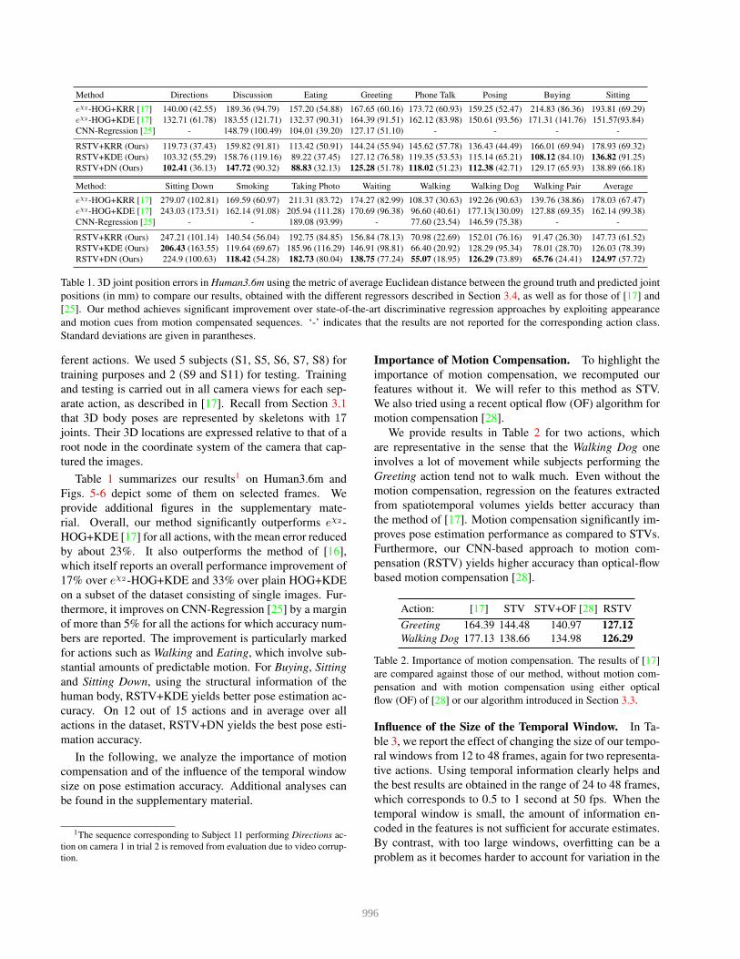
Table 1. 3D joint position errors in Human3.6m using the metric of average Euclidean distance between the ground truth and predicted joint

positions (in mm) to compare our results, obtained with the different regressors described in Section 3.4, as well as for those of [17] and

[25]. Our method achieves significant improvement over state-of-the-art discriminative regression approaches by exploiting appearance

and motion cues from motion compensated sequences. ‘-’ indicates that the results are not reported for the corresponding action class.

Standard deviations are given in parantheses.

ferent actions. We used 5 subjects (S1, S5, S6, S7, S8) for

training purposes and 2 (S9 and S11) for testing. Training

and testing is carried out in all camera views for each sep-

arate action, as described in [17]. Recall from Section 3.1

that 3D body poses are represented by skeletons with 17joints. Their 3D locations are expressed relative to that of a

root node in the coordinate system of the camera that cap-

tured the images.

Table 1 summarizes our results1 on Human3.6m and

Figs. 5-6 depict some of them on selected frames. We

provide additional figures in the supplementary mate-

rial. Overall, our method significantly outperforms eχ2 -

HOG+KDE [17] for all actions, with the mean error reduced

by about 23%. It also outperforms the method of [16],

which itself reports an overall performance improvement of

17% over eχ2 -HOG+KDE and 33% over plain HOG+KDE

on a subset of the dataset consisting of single images. Fur-

thermore, it improves on CNN-Regression [25] by a margin

of more than 5% for all the actions for which accuracy num-

bers are reported. The improvement is particularly marked

for actions such as Walking and Eating, which involve sub-

stantial amounts of predictable motion. For Buying, Sitting

and Sitting Down, using the structural information of the

human body, RSTV+KDE yields better pose estimation ac-

curacy. On 12 out of 15 actions and in average over all

actions in the dataset, RSTV+DN yields the best pose esti-

mation accuracy.

In the following, we analyze the importance of motion

compensation and of the influence of the temporal window

size on pose estimation accuracy. Additional analyses can

be found in the supplementary material.

1The sequence corresponding to Subject 11 performing Directions ac-

tion on camera 1 in trial 2 is removed from evaluation due to video corrup-

tion.

Importance of Motion Compensation. To highlight the

importance of motion compensation, we recomputed our

features without it. We will refer to this method as STV.

We also tried using a recent optical flow (OF) algorithm for

motion compensation [28].

We provide results in Table 2 for two actions, which

are representative in the sense that the Walking Dog one

involves a lot of movement while subjects performing the

Greeting action tend not to walk much. Even without the

motion compensation, regression on the features extracted

from spatiotemporal volumes yields better accuracy than

the method of [17]. Motion compensation significantly im-

proves pose estimation performance as compared to STVs.

Furthermore, our CNN-based approach to motion com-

pensation (RSTV) yields higher accuracy than optical-flow

based motion compensation [28].

Action: [17] STV STV+OF [28] RSTV

Greeting 164.39 144.48 140.97 127.12

Walking Dog 177.13 138.66 134.98 126.29

Table 2. Importance of motion compensation. The results of [17]

are compared against those of our method, without motion com-

pensation and with motion compensation using either optical

flow (OF) of [28] or our algorithm introduced in Section 3.3.

Influence of the Size of the Temporal Window. In Ta-

ble 3, we report the effect of changing the size of our tempo-

ral windows from 12 to 48 frames, again for two representa-

tive actions. Using temporal information clearly helps and

the best results are obtained in the range of 24 to 48 frames,

which corresponds to 0.5 to 1 second at 50 fps. When the

temporal window is small, the amount of information en-

coded in the features is not sufficient for accurate estimates.

By contrast, with too large windows, overfitting can be a

problem as it becomes harder to account for variation in the

996

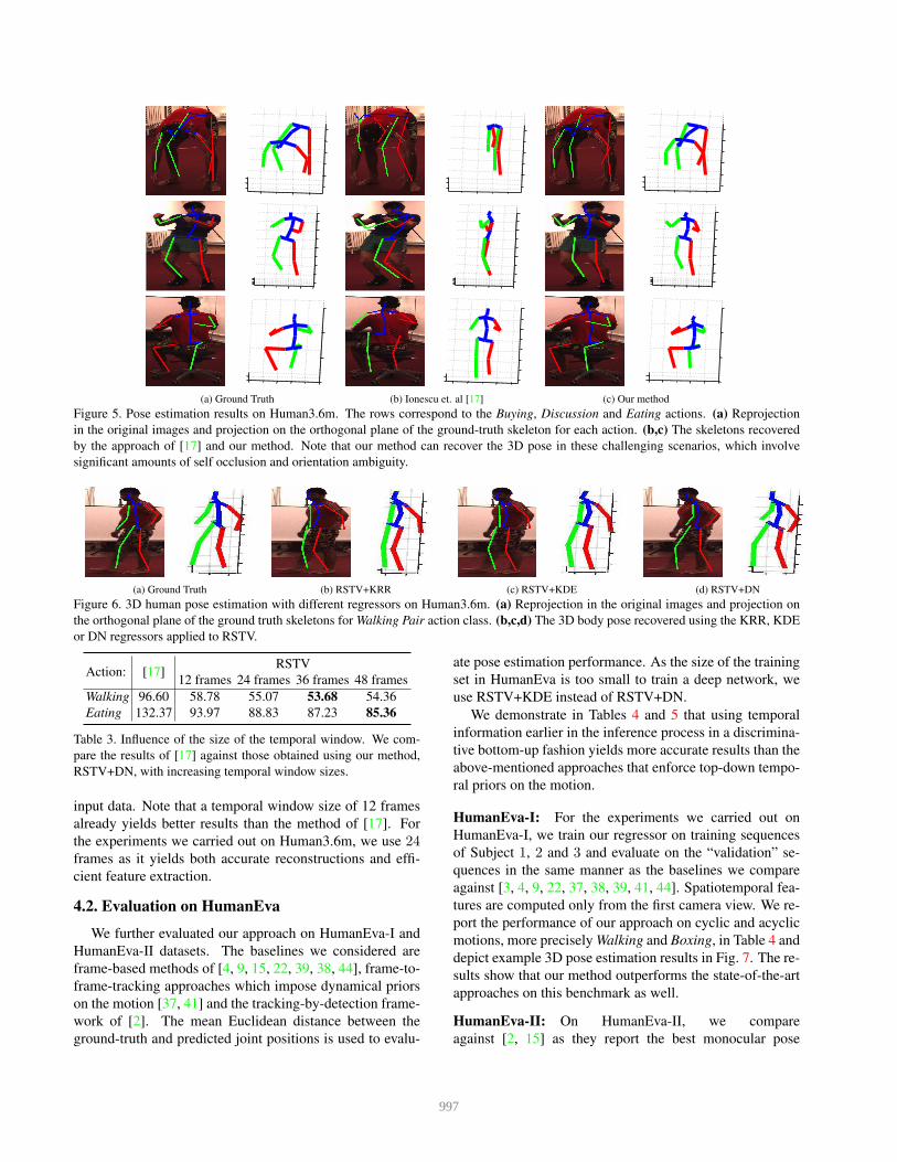
(a) Ground Truth (b) Ionescu et. al [17] (c) Our method

Figure 5. Pose estimation results on Human3.6m. The rows correspond to the Buying, Discussion and Eating actions. (a) Reprojection

in the original images and projection on the orthogonal plane of the ground-truth skeleton for each action. (b,c) The skeletons recovered

by the approach of [17] and our method. Note that our method can recover the 3D pose in these challenging scenarios, which involve

significant amounts of self occlusion and orientation ambiguity.

(a) Ground Truth (b) RSTV+KRR (c) RSTV+KDE (d) RSTV+DN

Figure 6. 3D human pose estimation with different regressors on Human3.6m. (a) Reprojection in the original images and projection on

the orthogonal plane of the ground truth skeletons for Walking Pair action class. (b,c,d) The 3D body pose recovered using the KRR, KDE

or DN regressors applied to RSTV.

Action: [17]RSTV

12 frames 24 frames 36 frames 48 frames

Walking 96.60 58.78 55.07 53.68 54.36

Eating 132.37 93.97 88.83 87.23 85.36

Table 3. Influence of the size of the temporal window. We com-

pare the results of [17] against those obtained using our method,

RSTV+DN, with increasing temporal window sizes.

input data. Note that a temporal window size of 12 frames

already yields better results than the method of [17]. For

the experiments we carried out on Human3.6m, we use 24frames as it yields both accurate reconstructions and effi-

cient feature extraction.

4.2. Evaluation on HumanEva

We further evaluated our approach on HumanEva-I and

HumanEva-II datasets. The baselines we considered are

frame-based methods of [4, 9, 15, 22, 39, 38, 44], frame-to-

frame-tracking approaches which impose dynamical priors

on the motion [37, 41] and the tracking-by-detection frame-

work of [2]. The mean Euclidean distance between the

ground-truth and predicted joint positions is used to evalu-

ate pose estimation performance. As the size of the training

set in HumanEva is too small to train a deep network, we

use RSTV+KDE instead of RSTV+DN.

We demonstrate in Tables 4 and 5 that using temporal

information earlier in the inference process in a discrimina-

tive bottom-up fashion yields more accurate results than the

above-mentioned approaches that enforce top-down tempo-

ral priors on the motion.

HumanEva-I: For the experiments we carried out on

HumanEva-I, we train our regressor on training sequences

of Subject 1, 2 and 3 and evaluate on the “validation” se-

quences in the same manner as the baselines we compare

against [3, 4, 9, 22, 37, 38, 39, 41, 44]. Spatiotemporal fea-

tures are computed only from the first camera view. We re-

port the performance of our approach on cyclic and acyclic

motions, more precisely Walking and Boxing, in Table 4 and

depict example 3D pose estimation results in Fig. 7. The re-

sults show that our method outperforms the state-of-the-art

approaches on this benchmark as well.

HumanEva-II: On HumanEva-II, we compare

against [2, 15] as they report the best monocular pose

997

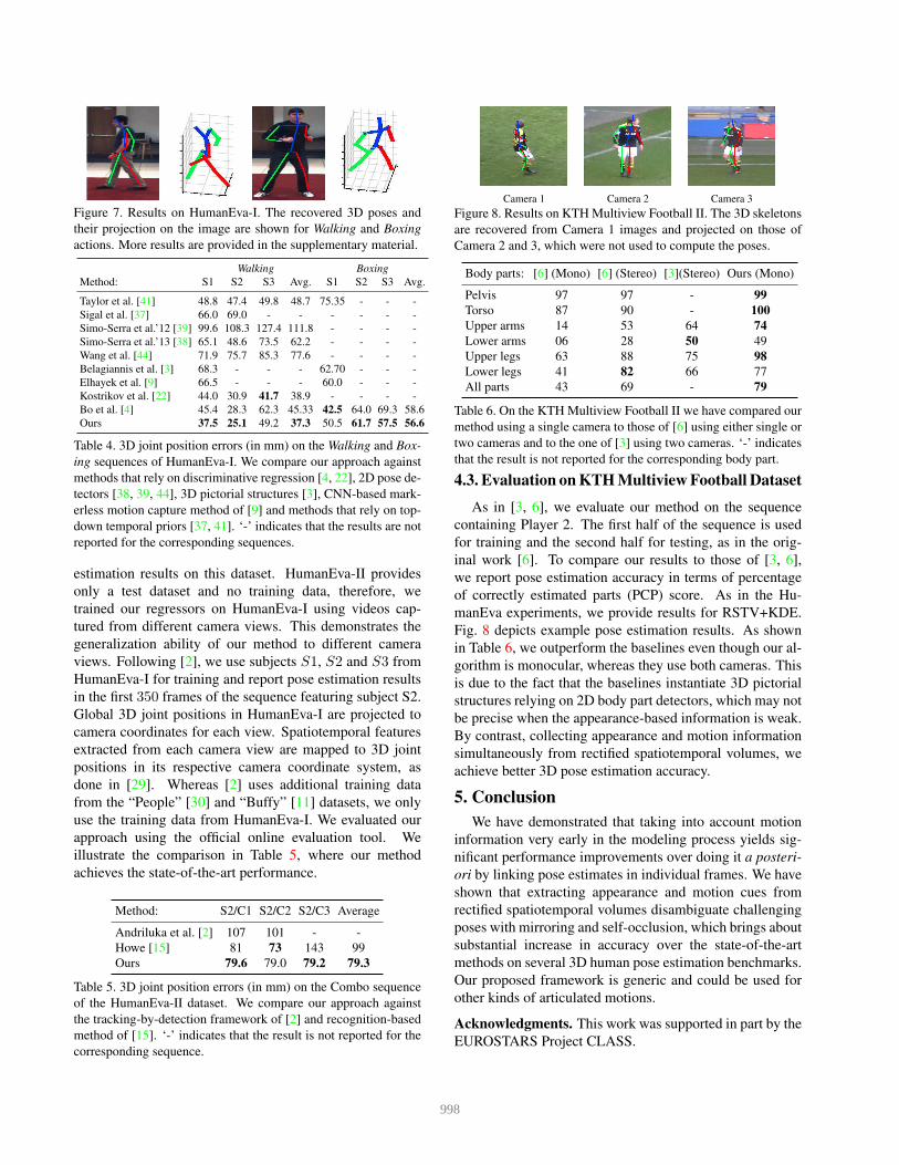
Figure 7. Results on HumanEva-I. The recovered 3D poses and

their projection on the image are shown for Walking and Boxing

actions. More results are provided in the supplementary material.

Walking Boxing

Method: S1 S2 S3 Avg. S1 S2 S3 Avg.

Taylor et al. [41] 48.8 47.4 49.8 48.7 75.35 - - -

Sigal et al. [37] 66.0 69.0 - - - - - -

Simo-Serra et al.’12 [39] 99.6 108.3 127.4 111.8 - - - -

Simo-Serra et al.’13 [38] 65.1 48.6 73.5 62.2 - - - -

Wang et al. [44] 71.9 75.7 85.3 77.6 - - - -

Belagiannis et al. [3] 68.3 - - - 62.70 - - -

Elhayek et al. [9] 66.5 - - - 60.0 - - -

Kostrikov et al. [22] 44.0 30.9 41.7 38.9 - - - -

Bo et al. [4] 45.4 28.3 62.3 45.33 42.5 64.0 69.3 58.6

Ours 37.5 25.1 49.2 37.3 50.5 61.7 57.5 56.6

Table 4. 3D joint position errors (in mm) on the Walking and Box-

ing sequences of HumanEva-I. We compare our approach against

methods that rely on discriminative regression [4, 22], 2D pose de-

tectors [38, 39, 44], 3D pictorial structures [3], CNN-based mark-

erless motion capture method of [9] and methods that rely on top-

down temporal priors [37, 41]. ‘-’ indicates that the results are not

reported for the corresponding sequences.

estimation results on this dataset. HumanEva-II provides

only a test dataset and no training data, therefore, we

trained our regressors on HumanEva-I using videos cap-

tured from different camera views. This demonstrates the

generalization ability of our method to different camera

views. Following [2], we use subjects S1, S2 and S3 from

HumanEva-I for training and report pose estimation results

in the first 350 frames of the sequence featuring subject S2.

Global 3D joint positions in HumanEva-I are projected to

camera coordinates for each view. Spatiotemporal features

extracted from each camera view are mapped to 3D joint

positions in its respective camera coordinate system, as

done in [29]. Whereas [2] uses additional training data

from the “People” [30] and “Buffy” [11] datasets, we only

use the training data from HumanEva-I. We evaluated our

approach using the official online evaluation tool. We

illustrate the comparison in Table 5, where our method

achieves the state-of-the-art performance.

Method: S2/C1 S2/C2 S2/C3 Average

Andriluka et al. [2] 107 101 - -

Howe [15] 81 73 143 99

Ours 79.6 79.0 79.2 79.3

Table 5. 3D joint position errors (in mm) on the Combo sequence

of the HumanEva-II dataset. We compare our approach against

the tracking-by-detection framework of [2] and recognition-based

method of [15]. ‘-’ indicates that the result is not reported for the

corresponding sequence.

Camera 1 Camera 2 Camera 3

Figure 8. Results on KTH Multiview Football II. The 3D skeletons

are recovered from Camera 1 images and projected on those of

Camera 2 and 3, which were not used to compute the poses.

Body parts: [6] (Mono) [6] (Stereo) [3](Stereo) Ours (Mono)

Pelvis 97 97 - 99

Torso 87 90 - 100

Upper arms 14 53 64 74

Lower arms 06 28 50 49

Upper legs 63 88 75 98

Lower legs 41 82 66 77

All parts 43 69 - 79

Table 6. On the KTH Multiview Football II we have compared our

method using a single camera to those of [6] using either single or

two cameras and to the one of [3] using two cameras. ‘-’ indicates

that the result is not reported for the corresponding body part.

4.3. Evaluation on KTH Multiview Football Dataset

As in [3, 6], we evaluate our method on the sequence

containing Player 2. The first half of the sequence is used

for training and the second half for testing, as in the orig-

inal work [6]. To compare our results to those of [3, 6],

we report pose estimation accuracy in terms of percentage

of correctly estimated parts (PCP) score. As in the Hu-

manEva experiments, we provide results for RSTV+KDE.

Fig. 8 depicts example pose estimation results. As shown

in Table 6, we outperform the baselines even though our al-

gorithm is monocular, whereas they use both cameras. This

is due to the fact that the baselines instantiate 3D pictorial

structures relying on 2D body part detectors, which may not

be precise when the appearance-based information is weak.

By contrast, collecting appearance and motion information

simultaneously from rectified spatiotemporal volumes, we

achieve better 3D pose estimation accuracy.

5. Conclusion

We have demonstrated that taking into account motion

information very early in the modeling process yields sig-

nificant performance improvements over doing it a posteri-

ori by linking pose estimates in individual frames. We have

shown that extracting appearance and motion cues from

rectified spatiotemporal volumes disambiguate challenging

poses with mirroring and self-occlusion, which brings about

substantial increase in accuracy over the state-of-the-art

methods on several 3D human pose estimation benchmarks.

Our proposed framework is generic and could be used for

other kinds of articulated motions.

Acknowledgments. This work was supported in part by the

EUROSTARS Project CLASS.

998

References

[1] A. Agarwal and B. Triggs. 3D Human Pose from Silhouettes

by Relevance Vector Regression. In CVPR, 2004.

[2] M. Andriluka, S. Roth, and B. Schiele. Monocular 3D Pose

Estimation and Tracking by Detection. In CVPR, 2010.

[3] V. Belagiannis, S. Amin, M. Andriluka, B. Schiele,

N. Navab, and S. Ilic. 3D Pictorial Structures for Multiple

Human Pose Estimation. In CVPR, 2014.

[4] L. Bo and C. Sminchisescu. Twin Gaussian Processes for

Structured Prediction. IJCV, 2010.

[5] J. Brauer, W. Gong, J. Gonzalez, and M. Arens. On the Ef-

fect of Temporal Information on Monocular 3D Human Pose

Estimation. In ICCV, 2011.

[6] M. Burenius, J. Sullivan, and S. Carlsson. 3D Pictorial Struc-

tures for Multiple View Articulated Pose Estimation. In

CVPR, 2013.

[7] X. Burgos-Artizzu, D. Hall, P. Perona, and P. Dollar. Merg-

ing Pose Estimates Across Space and Time. In BMVC, 2013.

[8] C. Cortes, M. Mohri, and J. Weston. A General Regression

Technique for Learning Transductions. In ICML, 2005.

[9] A. Elhayek, E. Aguiar, A. Jain, J. Tompson, L. Pishchulin,

M. Andriluka, C. Bregler, B. Schiele, and C. Theobalt. Ef-

ficient Convnet-Based Marker-Less Motion Capture in Gen-

eral Scenes with a Low Number of Cameras. In CVPR, 2015.

[10] P. Felzenszwalb, R. Girshick, D. McAllester, and D. Ra-

manan. Object Detection with Discriminatively Trained Part

Based Models. PAMI, 2010.

[11] V. Ferrari, M. Martin, and A. Zisserman. Progressive Search

Space Reduction for Human Pose Estimation. In CVPR,

2008.

[12] J. Gall, B. Rosenhahn, T. Brox, and H.-P. Seidel. Optimiza-

tion and Filtering for Human Motion Capture. IJCV, 2010.

[13] S. Gammeter, A. Ess, T. Jaeggli, K. Schindler, B. Leibe, and

L. Van Gool. Articulated Multi-Body Tracking Under Ego-

motion. In ECCV, 2008.

[14] T. Hofmann, B. Schlkopf, and A. J. Smola. Kernel Methods

in Machine Learning. The Annals of Statistics, 2008.

[15] N. R. Howe. A Recognition-Based Motion Capture Baseline

on the Humaneva II Test Data. MVA, 2011.

[16] C. Ionescu, J. Carreira, and C. Sminchisescu. Iterated

Second-Order Label Sensitive Pooling for 3D Human Pose

Estimation. In CVPR, 2014.

[17] C. Ionescu, I. Papava, V. Olaru, and C. Sminchisescu. Hu-

man3.6M: Large Scale Datasets and Predictive Methods for

3D Human Sensing in Natural Environments. PAMI, 2014.

[18] A. Kanaujia, C. Sminchisescu, and D. N. Metaxas. Semi-

Supervised Hierarchical Models for 3D Human Pose Recon-

struction. In CVPR, 2007.

[19] A. Karpathy, G. Toderici, S. Shetty, T. Leung, R. Sukthankar,

and L. Fei-Fei. Large-Scale Video Classification with Con-

volutional Neural Networks. In CVPR, 2014.

[20] D. Kingma and J. Ba. Adam: A Method for Stochastic Opti-

misation. In ICLR, 2015.

[21] A. Klaser, M. Marszałek, and C. Schmid. A Spatio-Temporal

Descriptor Based on 3D-Gradients. In BMVC, 2008.

[22] I. Kostrikov and J. Gall. Depth Sweep Regression Forests for

Estimating 3D Human Pose from Images. In BMVC, 2014.

[23] I. Laptev. On Space-Time Interest Points. IJCV, 2005.

[24] F. Li, G. Lebanon, and C. Sminchisescu. Chebyshev Ap-

proximations to the Histogram χ2 Kernel. In CVPR, 2012.

[25] S. Li and A. B. Chan. 3D Human Pose Estimation from

Monocular Images with Deep Convolutional Network. In

ACCV, 2014.

[26] E. Mansimov, N. Srivastava, and R. Salakhutdinov. Initial-

ization Strategies of Spatio-Temporal Convolutional Neural

Networks. CoRR, abs/1503.07274, 2015.

[27] D. Ormoneit, H. Sidenbladh, M. Black, T. Hastie, and

D. Fleet. Learning and Tracking Human Motion Using Func-

tional Analysis. In IEEE Workshop on Human Modeling,

Analysis and Synthesis, 2000.

[28] D. Park, C. L. Zitnick, D. Ramanan, and P. Dollar. Exploring

Weak Stabilization for Motion Feature Extraction. In CVPR,

2013.

[29] R. Poppe. Evaluating Example-Based Pose Estimation: Ex-

periments on the Humaneva Sets. In CVPR, 2007.

[30] D. Ramanan. Learning to Parse Images of Articulated Bod-

ies. In NIPS, 2006.

[31] D. Ramanan, A. Forsyth, and A. Zisserman. Strike a Pose:

Tracking People by Finding Stylized Poses. In CVPR, 2005.

[32] A. Rozantsev, V. Lepetit, and P. Fua. Flying Objects Detec-

tion from a Single Moving Camera. In CVPR, 2015.

[33] B. Sapp, A. Toshev, and B. Taskar. Cascaded Models for

Articulated Pose Estimation. In ECCV, 2010.

[34] J. Shotton, A. Fitzgibbon, M. Cook, and A. Blake. Real-

Time Human Pose Recognition in Parts from a Single Depth

Image. In CVPR, 2011.

[35] H. Sidenbladh, M. J. Black, and D. J. Fleet. Stochastic

Tracking of 3D Human Figures Using 2D Image Motion. In

ECCV, 2000.

[36] L. Sigal, A. Balan, and M. J. Black. Humaneva: Synchro-

nized Video and Motion Capture Dataset and Baseline Algo-

rithm for Evaluation of Articulated Human Motion. IJCV,

2010.

[37] L. Sigal, M. Isard, H. W. Haussecker, and M. J. Black.

Loose-Limbed People: Estimating 3D Human Pose and Mo-

tion Using Non-Parametric Belief Propagation. IJCV, 2012.

[38] E. Simo-Serra, A. Quattoni, C. Torras, and F. Moreno-

Noguer. A Joint Model for 2D and 3D Pose Estimation from

a Single Image. In CVPR, 2012.

[39] E. Simo-Serra, A. Ramisa, G. Alenya, C. Torras, and

F. Moreno-Noguer. Single Image 3D Human Pose Estima-

tion from Noisy Observations. In CVPR, 2012.

[40] C. Sminchisescu, A. Kanaujia, Z. Li, and D. Metaxas. Dis-

criminative Density Propagation for 3D Human Motion Es-

timation. In CVPR, 2005.

[41] G. W. Taylor, L. Sigal, D. J. Fleet, and G. E. Hinton. Dy-

namical Binary Latent Variable Models for 3D Human Pose

Tracking. In CVPR, 2010.

[42] R. Urtasun and T. Darrell. Sparse Probabilistic Regression

for Activity-Independent Human Pose Inference. In CVPR,

2008.

999

[43] R. Urtasun, D. Fleet, A. Hertzman, and P. Fua. Priors for

People Tracking from Small Training Sets. In ICCV, 2005.

[44] C. Wang, Y. Wang, Z. Lin, A. L. Yuille, and W. Gao. robust

Estimation of 3D Human Poses from a Single Image.

[45] D. Weinland, M. Ozuysal, and P. Fua. Making Action Recog-

nition Robust to Occlusions and Viewpoint Changes. In

ECCV, 2010.

[46] F. Zhou and F. de la Torre. Spatio-Temporal Matching for

Human Detection in Video. In ECCV, 2014.

[47] S. Zuffi, J. Romero, C. Schmid, and M. J. Black. Estimating

Human Pose with Flowing Puppets. In ICCV, 2013.

1000