Direct, indirect, and composition effects of monetary

Direct, indirect, and composition effects ofmonetary interventions?

James S. Cloyne † Oscar Jorda‡ Alan M. Taylor §

March 2018

DO NOT CIRCULATE WITHOUT PERMISSION FROM THE AUTHORS

Abstract

Impulse responses trace the average effect of a policy intervention on a macroeconomicoutcome over time. Using local projections, this dynamic average effect can be decom-posed three ways as: (1) the direct effect of the intervention on the outcome; (2) theindirect effect due to changes in how other covariates affect the outcome when there is anintervention; and (3) a composition effect due to differences in covariates between treatedand control subpopulations. This Blinder-Oaxaca-type decomposition of the impulseresponse provides convenient ways to evaluate the effects of policy, state-dependence,and balance conditions for identification.

JEL classification codes: E01, E30, E32, E44, E47, E51, F33, F42, F44

Keywords: Blinder-Oaxaca decomposition, local projections, interest rates, monetarypolicy, state-dependence, balance, identification.

?We thank Chitra Marti for excellent research assistance. The views expressed in this paper are the soleresponsibility of the authors and to not necessarily reflect the views of the Federal Reserve Bank of SanFrancisco or the Federal Reserve System.

†Department of Economics, University of California, Davis; and CEPR ().‡Federal Reserve Bank of San Francisco; and Department of Economics, University of California, Davis

([email protected]; [email protected]).§Department of Economics and Graduate School of Management, University of California, Davis; NBER;

and CEPR ([email protected]).

mailto:[email protected]




1. Introduction

An accurate measure of exogenous movements (or interventions) in monetary policy may not be

enough to empirically evaluate its effects on economic outcomes. There are at least two reasons why

this may be the case. First, in small samples, there can be differences in average economic conditions

between the subpopulations implicitly defined by whether or not there is an intervention, even if in

large samples these differences would vanish under appropriate identification. Failure to sterilize

this lack of balance will bias estimates of the impulse response. Second, interventions can affect

how other variables affect the outcomes. The impulse response will then conflate this indirect effect

with the direct effect of the intervention itself. Traditional estimates of impulse responses, such as

those based on vector autoregressions or VARs, implicitly assume that these two effects are zero.

We show that this is far from being the case in the data and what to do about it. Our paper thus

explains how to correct for these distortions and thus obtain an accurate measure of the effect of

monetary policy interventions.

Empirical impulse responses are diagnostic statistics of those economic mechanisms most likely

to explain the data. They are routinely used to evaluate alternative macroeconomic models of the

business cycle. Not unlike medical trials, randomly assigned (unsystematic and unanticipated)

interventions—the impulse—are the surest way to avoid confounding from alternative sources,

whether observable or not. The literature has therefore dedicated considerable effort to obtaining

such exogenous monetary interventions. Recent examples include Gurkaynak, Sack, and Swanson

(2005), Gertler and Karadi (2015), Miranda-Agrippino (2015), and Ramey (2016), among several

others. Our particular focus here will be on an updated version of Romer and Romer (2004)

constructed by Cloyne and Hurtgen (2016). The reason we use this series of monetary shocks is that

they will provide for a well-accepted benchmark for our experiments.

Impulse responses can be interpreted as the dynamic counterpart of the ubiquitous average

treatment effect reported in applied economics. In a typical randomized controlled trial, the

average treatment effect compares the counterfactual expectation of the outcome variable under

intervention (the treatment subpopulation) with the expectation absent intervention (the control

subpopulation), both conditional on observable information. Impulse responses can similarly be

seen as the difference between a counterfactual and its forecast—which is a conditional expectation.

Thus, a natural and convenient way to compute impulse responses is via local projections (Jorda,

2005).

Specifically, the decomposition methods that we introduce take the local approach in Jorda (2005)

and extends it to be able to carry out the well-known Blinder-Oaxaca decomposition (Blinder, 1973;

Oaxaca, 1973). This decomposition is standard in applied microeconomics (Fortin, Lemieux, and

Firpo, 2011), but until now had not found equivalent acceptance in applied macroeconomics.

Extending the local projections framework in this manner turns out to be trivially simple.

1

Estimation and inference can be obtained by standard linear regression methods. Yet the extension

is sufficiently general to allow for a great deal of unspecified state-dependence. Given the current

state of the economy, in our case simply characterized by interest rates, inflation and economic

activity, a 25 basis point increase in the federal funds rate target can have very different effects.

Using historical episodes to characterize states of interest, we reexamine long-standing explanations

on the effectiveness of monetary policy.

We believe that although the new methods introduced here are an important refinement over

long-standing views on how monetary economies work, they have their limitations. As Fortin et al.

(2011), the Blinder-Oaxaca decomposition inherently follows a partial equilibrium approach. For

example, it is not correct to infer how much more or less effective monetary policy would be if, say,

fiscal policy actively pursued a reduction of public debt to 30% of GDP. Instead, the decomposition

measures differences in monetary policy effectiveness by averaging across alternative historical

episodes whose make-up it takes as given. In that regard, it is not different than if one were to try

to extrapolate from an impulse response what the appropriate course of action is for the monetary

authority. Our analysis is not normative. That said, there may situations where external instruments

are available to identify these alternative channels but they are not explicitly explored in this paper.

Using the new methods that we introduce here, we begin by replicating estimates of the responses

of economic activity, inflation, and interest rates reported in Romer and Romer (2004) using local

projections. These estimates serve as benchmarks and indeed confirm the findings in Romer and

Romer (2004). Still within the traditional framework, we show that there exist differences in the

treated and control subpopulations. These differences generate bias in traditional estimates of

impulse responses and we show what the corrected responses look like.

Next we go one step further. Using a Blinder-Oaxaca specification, we extend the analysis

and decompose these responses into composition, indirect, and direct effects of a monetary policy

intervention. We show that composition effects attenuate the activity response to an increase in the

funds rate, but accentuate the response of inflation. At the mean, the indirect effect is relatively small,

perhaps explaining why studies based on VARs have usually found little evidence of neglected

non-linearities. However, deviations from sample averages affect the shape of the responses greatly,

as we show.

We pursue this question further by examining selected historical episodes. We examine the

month following the stock market crash of 1987. The funds rate was lowered by 50 basis points in

response to the crash. Yet we show that such a reaction would be expected to have a much more

muted effect on economic activity than it did on average historically. In contrast, in 1996, about the

half way point of a long expansion and with productivity on the upswing, we find, perhaps not

surprisingly, that policy actions would have a smaller effect on prices despite affecting economic

activity almost the same as historically.

To sum up, we view our paper as making two types of contribution, one methodological, the

other furthering our understanding of how monetary economies behave. On the methodological

front we show that with a relatively straightforward extension of the local projection approach, one

2

can gain tremendous insight from the data. We expect that these methods will be particularly useful

in other applications and that they will be extended in a variety of ways.

2. Preliminary statistical discussion and intuition

When it comes to investigating causal relationships, randomized controlled trials are generally

viewed as the gold standard of scientific research. We briefly discuss some basic ideas based on

this paradigm to motivate the local projection decomposition that we introduce later on. We forgo

being too precise about the assumptions needed here, instead preferring to focus on the intuition.

Formal statements of any assumptions needed can be found in, e. g., Wooldridge (2001) and Fortin

et al. (2011). For now assume that treatment s ∈ {0, 1} is randomly assigned, at least conditional on

controls x.

Suppose that we are interested in the response of an outcome variable, y, to a randomly assignedintervention, s. The observed data are therefore generated by:

y = (1− s) y0 + s y1 = y0 + s (y1 − y0). (1)

That is, the observed random variable y is either the random variable y0, which is observed when

s = 0, or it is the random variable y1 when s = 1. Note that y0, y1 are potential outcomes in the

terminology of the Rubin causal model (Rubin, 1974). The random variables yj with j ∈ {0, 1} have

unconditional mean E(yj) = µj. A natural statistic of interest is E(y1 − y0) = µ1 − µ0, that is, the

average difference in the unconditional mean between the treated and the control subpopulations.

Note that the data can be observed in one state or the other, but we never get to observe a realization

of these random variables in both states simultaneously.

The potential outcomes notation can be somewhat new to applied macroeconomists. A few

examples can help clarify basic notions. In a randomized controlled trial, a common (strong)

ignorability assumption is that yj ⊥ s for j = 0, 1. This assumption does not imply that y and sare unrelated to one another. We are not assuming that there is no treatment effect. Rather, the

assumption means that the choice of intervention s is unrelated to the potential outcomes that may

happen for a given choice of s ∈ {0, 1}. For this reason, a quantity such as E(y1|s = 0) is well defined.

It refers to the expected value that the random variable y1—from the treated subpopulation—would

counterfactually take if it were not exposed to treatment. We will use such counterfactual expectations

below.

2.1. The Blinder-Oaxaca decomposition

Without loss of generality, we can write yj = µj + vj where E(vj) = 0 since E(yj) = µj by definition.

Any heterogeneity in the treated and control subpopulations is therefore relegated to the terms vj.

Whenever covariates (explanatory variables or simply, controls) x are available, they are useful to

3

characterize heterogeneity across units (and later for us, across time) and we may assume additivity

so that vj = g(x) + εj. As a starting point it is natural to further assume that these covariates

enter linearly, so that vj = (x− E(x))γj + εj. We include the covariates in deviations from their

unconditional mean to ensure that E[(x− E(x))γj] = 0, in which case unobserved heterogeneity

is such that E(εj) = 0. If observed heterogeneity is well captured by the vector of explanatory

variables and the linearity assumption is correct, then it is also the case that E(εj|xj) = 0. That is,

the projection of yj onto xj is properly specified.

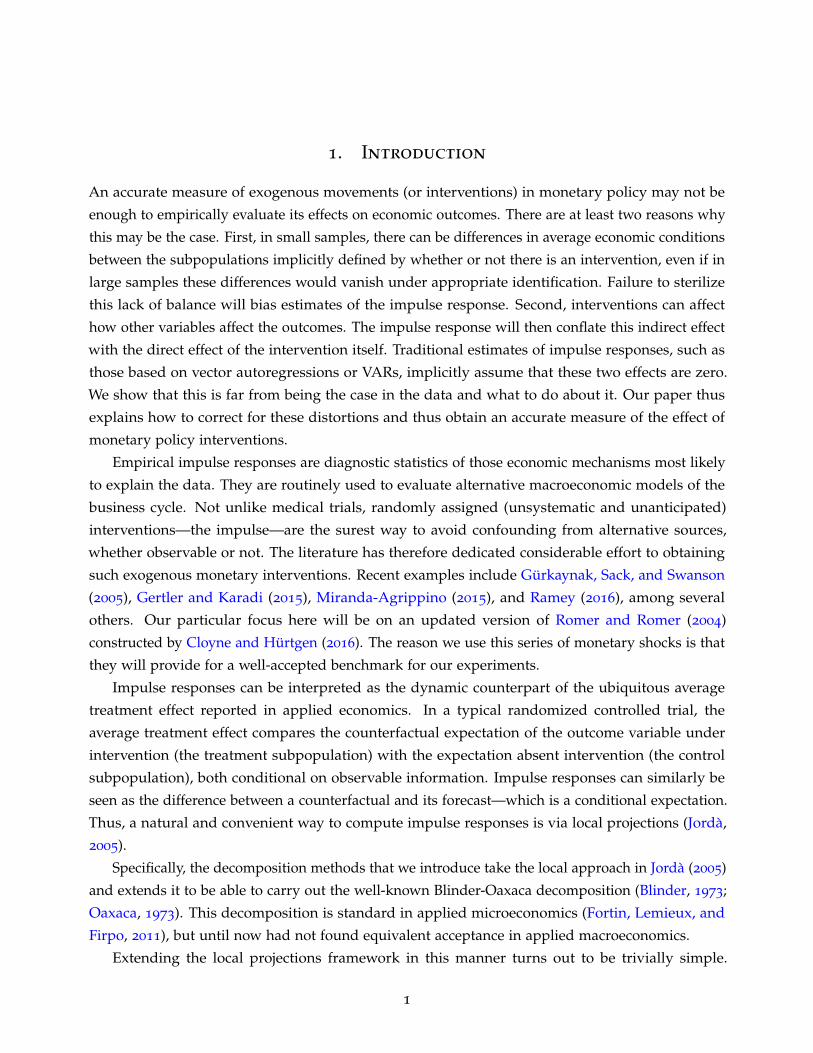
Researchers are often interested in understanding the overall effect on the intervention on

outcomes. The Blinder-Oaxaca decomposition (Blinder, 1973; Oaxaca, 1973) is used often in applied

microeconomics for this purpose. It is worth going through its derivation here before later using

similar arguments on local projections. These derivations borrow heavily from Wooldridge (2001)

and Fortin et al. (2011). The overall effect of the intervention can be written as:

E(y1|s = 1)− E(y0|s = 0) = E[E(y1|x, s = 1)|s = 1]− E[E(y0|x, s = 0)|s = 0]

= µ1 + E[x− E(x)|s = 1]γ1 + E(ε1|s = 1)︸︷︷︸=0

− {µ0 + E[x− E(x)|s = 0]γ0 + E(ε0|s = 0)︸︷︷︸=0

}. (2)

Adding and subtracting E[x− E(x)|s = 1]γ0, expression (2) can be rearranged as follows:

E(y1|s = 1)− E(y0|s = 0) = (µ1 − µ0)

+ E[x− E(x)|s = 1](γ1 − γ0)

+ {E[x− E(x)|s = 1]− E[x− E(x)|s = 0]}γ0 (3)

Expression (3) contains three interesting elements. The term µ1 − µ0, refers to the difference in the

unconditional means of the treated and control subpopulations and we refer to it as the direct effect

of an intervention.

The term E[x− E(x)|s = 1](γ1 − γ0) reflects changes in how the covariates affect the outcome

due to the intervention. We will refer to this term as the indirect effect of intervention. For example,

a background in mathematics may translate into a higher salary for workers assigned to take

additional training in computer science, but may not otherwise (or at least not to the same extent

if there is a complementarity between both knowing mathematics and computer science). Notice

that E[x− E(x)|s = 1]γ0 explores the salary of workers with a given background in mathematics,

had they been counterfactually assigned not to take the additional training in computer science. A

natural hypothesis we will be interested in testing is H0 : γ1 − γ0 = 0. Failure to reject the null

suggests that the effect of the covariates on the outcome is not affected by the intervention. It turns

4

out that traditional estimates of impulse responses implicitly assume this to be the case. Later on we

will see that such a hypothesis plays a critical role in evaluating impulse response state-dependence.

The final term, {E[x− E(x)|s = 1]− E[x− E(x)|s = 0]}γ0 indicates that, all else equal, the effect

of intervention may be driven simply by differences in the average value of the explanatory variables

between the treated and control subpopulations. We will call this term, the composition effect. A

test of the null H0 : E[x− E(x)|s = 1]− E[x− E(x)|s = 0] = 0→ H0 : E[x|s = 1]− E[x|s = 0] = 0

is useful to determine the balance of the distribution of covariates between treated and control

subpopulations. In a randomized control trial, there should be no differences and the null would not

be rejected. A rejection of the null instead indicates that selection into treatment could depend on

the value of the covariates and hence introduce selection bias in the estimation. Thus, a test of this

null can be used to detect potential failures of identification. In any case, small sample measurement

of the composition effect can be used to sterilize the impulse response.

In practice, a natural way to obtain each term in the decomposition of expression (3) given a

finite sample of N observations would be to estimate the following regression using expression (1)

as the sprinboard:

yi = µ0 + (xi − x)γ0 + si{β + (xi − x)θ}+ ωi (4)

where β = µ1− µ0 is an estimate of the direct effect; θ = γ1− γ0 and hence (x1− x)θ is an estimate

of the indirect effect. The notation x1 refers to the sample mean of the covariates for the treated

units. A test of the null H0 : θ = 0 is a test of the null that the indirect effect is zero and that the

covariates affect the outcomes in the same way whether or not a unit is treated. Finally, the term

(x1 − x0)γ0 is an estimate of the composition effect and a natural balance test is a test of the null

H0 : E(x|s = 1)− E(x|s = 0) = 0. Note that the error term is ωi = εi,0 + si(ε1,i − ε0,i). Under the

maintained assumptions, it has mean zero conditional on covariates.

3. Deconstructing the impulse response:

Direct, indirect, and composition effects

The methods discussed in Section 2, while common in applied microeconomics research, have not

permeated macroeconomics as much. In this section we show that local projections offer a natural

bridge between literatures and hence offer a more detailed understanding of impulse responses, the

workhorse of applied macroeconomics research.

In order to move from the preliminary statistical discussion to a time series setting in which to

investigate impulse responses, we define the outcome random variable observed h periods since

intervention as y(h) and a typical observation from a sample of T observations as yt+h. As before,

we begin with a binary policy intervention (earlier, the treatment) denoted s ∈ {0, 1} with a typical

observation from a finite sample denoted as st. A vector of observable predetermined variables is

5

denoted x, and an observation from a finite sample as xt. Note that x includes contemporaneous

values and lags of a vector of variables including the intervention, as well as lags of the (possibly

transformed) outcome variable, among others. Moreover, define y = (y(0), y(1), . . . , y(H)) or when

denoting an observation from a finite sample, yt = (yt, yt+1, . . . yt+H).

A natural natural starting point regarding the assignment of the policy intervention is to follow

Angrist, Jorda, and Kuersteiner (2016), whose selection on observable assumption we restate here

for convenience:

Assumption 1. Conditional ignorability or selection on observables. Let ys denote the potentialoutcome that the vector y can take on impact and up to H periods after intervention s ∈ {0, 1}. Then we says is randomly assigned conditional on x relative to y if:

ys ⊥ s|x for s = s(x, η;φ) ∈ {0, 1}; φ ∈ Φ.

This assumption makes explicit that the policy intervention s is itself a function the observables x,

unobservables η, and a parameter vector φ. The conditional ignorability assumption means that

ys ⊥ η, that is, the unobservables are random noise. Moreover, we assume that φ is constant for

the given sample considered. In other words, we rule out variation in the policy rule assigning

intervention.

Although such a general statement of conditional ignorability provides a great deal of flexibility

(see Angrist et al., 2016), a simpler assumption can be made when considering a linear framework

as we do in the analysis that follows. In particular, for our purposes, the following assumption will

suffice:

Assumption 2. Conditional mean independence. Let E(ys) = µs for s ∈ {0, 1} so that, without lossof generality, ys = µs + vs. As before, we now assume linearity so that vs = (x− E(x))Γs + εs. Becauseof the dimensions of ys, notice that Γs is now a matrix of coefficients with row dimension H + 1. Underconditional mean independence,

E(ys|x) = µs; E(vs) = 0; E(εs|x) = 0; s ∈ {0, 1} (5)

Based on Assumption 2, local projections can be easily extended to have the same format as

expression (4). Specifically:

yt+h = µh0 + (xt − x)γh

0 + st βh︸︷︷︸usual local projection

+ st (xt − x)θh︸︷︷︸Blinder-Oaxaca

+ωt+h; h = 0, 1, . . . , H; t = h, ..., T. (6)

That is, relative to the usual specification of a local projection, the only difference is the additional

term st(xt − x)θh. As a result of this simple extension, estimates of the components of an impulse

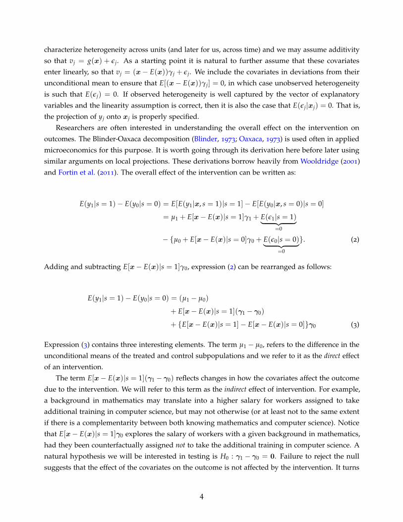
response can be calculated in parallel fashion to Section 2.1. That is:

6

Direct effect: µh1 − µh

0 = βh

Indirect effect: (x1 − x)(γh1 − γh

0 ) = (x1 − x)θh

Composition effect: (x1 − x0)γh0 (7)

where xs refers to the sample mean of the controls in each of the subpopulations s ∈ {0, 1}.In a time series context, one requires an assumption about the stationarity of the covariate

vector x. Without it, calculating means for the treated and control subpopulations would not be a

well-defined exercise. In a typical local projection it is not necessary to make such an assumption

because the parameter of interest is βh and all that is required for inference is for the projection to

have a sufficiently rich lag structure to ensure that the residuals are stationary. Consequently, we

now add the following assumption:

Assumption 3. Ergodicity. The vector of covariates xt—which can potentially include lagged values ofthe (possibly transformed) outcome variable and the treatment as well as current and lagged values of othervariables—is assumed to be a covariance-stationary vector process ergodic for the mean (see, e.g., Hamilton1994).

Ergodicity ensures that the sample mean converges to the population mean. Assuming covariance-

stationarity is a relatively standard way to ensure that this is the case. More general assumptions

could be made to accommodate less standard stochastic processes. However, covariance-stationarity

and ergodicity are sufficiently general to include many of the processes commonly observed in

practice.

3.1. Beyond binary policy interventions

Policy interventions sometimes vary from one intervention to the next. Think of monetary policy

and the different ways in which interest rates can be raised or lowered. Call it the problem of

choosing the policy dose. When the set of alternative doses is finite and small, it is easy to extend

the analysis from the Section 2 by defining s ∈ {s0, s1, ..., sJ} where s0 refers to the benchmark case

(e.g. s0 = 0) against which alternative treatments {s1, ..., sJ} are compared. An example of such an

approach in times series can be found in Angrist et al. (2016).

Investigating dose responses in this manner is advantageous. No assumption is made on possible

non-linear and non-monotonic effects of the treatment on the outcome. We know that, for example,

drugs administered in certain doses can be quite beneficial, but doubling the dose does not mean

that the benefit doubles—in fact, most drugs become lethal at higher and higher doses!

When doses vary continuously, say −∞ < δ < ∞, extending potential-outcomes ignorability

assumptions becomes impractical. There would be infinite potential outcomes (one for each value

of the dose received) and hence, we would be unable to recover parameters from finite samples.

7

However, with little loss of generality, we can assume that variation in doses affect outcomes through

a policy scaling factor δ = δ(x). The dependence of δ on x captures policy considerations and also

allows for non-monotonic effects in the choice of dose.

Under this more general form of δ, expression (1) now requires a further assumption regarding

the choice of dose given policy intervention in order to be able to identify the policy effect. A natural

assumption is conditional mean independence of the dose given assignment, which can be stated as

follows:

Assumption 4. Conditional mean independence of dose given assignment. As in Assumption 2,let ys = µs + vs with vs = (x− E(x))Γs + εs. Define the scaling factor δ(x). Then we assume that:

E[δ(x)y1|x) = δ(x)µ1,

that is, E[δ(x)ε1] = 0 since E[δ(x)(x− E(x))Γs|x] = 0 mechanically.

Notice that no further assumption is necessary regarding y0. Thus, Assumption 4 is a useful

reminder of the conditions required to explore impulse responses in general settings. Because this

paper introduces a number of novel elements, we will henceforth restrict the analysis to the case

where δ(x) = δ and leave for a different paper a more thorough investigation of non-monotonicities

in dose assignment. Such an assumption is no different than in standard VARs (e.g. Christiano,

Eichenbaum, and Evans, 1999)—doubling the dose, doubles the response. However, we think that

given the typical policy interventions observed, and given that outcomes are usually analyzed in

logarithms—so that policy interventions have proportional effects—this is a very reasonable starting

point. Based on this simplification, expression (4) can now be extended as follows:


0 + δt βh + δt(xt − x)θh + ωt+h; h = 0, 1, . . . , H; t = h, ..., T. (8)

using the convention δt = 0 if st = 0. The parameters βh and θh have the same interpretation as in

expression (6) in that scaling by the dosage allows one to interpret the coefficients on a per-unit-dose

basis. In the monetary policy application, this would correspond, say, to a 1 ppt increase in the

policy rate. Dividing by −4 would equivalently generate responses to a 0.25 bps decrease of the

policy rate instead. A constant scaling factor also implies symmetry. Importantly, the direct, indirect,

and composition effects can be estimated using estimates from the extended local projections in (8)

in the same manner as in the case of a binary treatment as explained in expression (7).

3.2. Blinder-Oaxaca state-dependent responses

An interesting feature of the Blinder-Oaxaca decomposition is that it allows us to evaluate the

indirect effect of the policy intervention at a particular value of the controls. For example, Angrist

8

et al. (2016) show that monetary policy loosening is less effective at stimulating the economy than

tightening. Tenreyro and Thwaites (2016) find asymmetric effects based on whether the economy

is in a boom or a bust. Jorda, Schularick, and Taylor (2017) report similar results using a different

approach and report that low inflation environments dull stimulative policy. These and many other

scenarios can be easily entertained using the Blinder-Oaxaca decomposition and the same set of

parameter estimates.

In particular, notice that:

E(y1|x∗, δ)− E(y0|x∗, s = 0) = δµ1 + δ[x∗ − E(x)]γ1 − {µ0 + [x∗ − E(x)]γ0}

= β + δ[x∗ − E(x)]θ, (9)

since E(δε1|x∗) = 0 and where x∗ refers to the specific value of x we wish to condition on.

Hence, based on the same estimates as those of the extended local projection in expression (8),

given x∗, the impulse response is:

δβ + δ(x∗ − x)θ (10)

for a given choice of δ since the composition effect is zero as [x∗ − x] is the same for the treated and

control subpopulations. Notice that we rely on the residuals having mean conditional on x of zero.

It is important to also note that because identification usually centers on treatment assignment rather

than identification for the controls, conditioning on certain values of x can only be interpreted from

a partial equilibrium perspective. Nevertheless, because in time series applications lagged values in

x are pre-determined with respect to the policy intervention, they are a legitimate description of a

state of the world in which we are interested in conducting a counterfactual experiment.

Several remarks are worth stating. First, although a convenient tool to investigate state-

dependence, note that given the assumptions we have made, the Blinder-Oaxaca decomposition

lacks enough information to evaluate how much more or less effective the impulse response indirect

effect would be if, say, the control xjt were to be made one unit bigger. The reason is that we have

made no assumptions about the assignment of the controls. We cannot infer causal effects about

them without further assumptions. The measured indirect effect for the jth control could be polluted

by any correlation with one or more other controls, for example.

Second, several hypotheses of interest underlie expression (7). Absence of direct effects can be

assessed by evaluating H0 : βh = 0; absence of indirect effects with H0 : φh = 0; and absence of

composition effects with H0 : γh0 = 0. All of these null hypotheses only require standard Wald tests

directly obtainable from standard regression output given our maintained assumptions. Thus formal

tests of economically meaningful hypotheses can be easily reported as we do in our application.

9

4. The direct effect of monetary policy

4.1. Replicating Romer and Romer (2004)

In monetary economies, a natural question of interest is to characterize the dynamic response of

economic activity, inflation and interest rates to an exogenous monetary intervention. Romer and

Romer (2004) provide a good place to start. We refer to their paper as RR from this point forward.

In their paper, they construct a series of exogenous monetary shocks by comparing actual changes

in the funds rate target with changes predicted by Federal Reserve Board staff. This series has

the advantage that it is directly observable and not the result of fitting any particular econometric

model. When introducing new methods, it is helpful to benchmark new findings against results that

have received wide acceptance in the literature.

The baseline regressions in RR are based on the following regression (and the same notation

used in their paper):

∆yt = a0 +1

∑k=1

akDkt +24

∑i=1

bi∆yt−i +36

∑j=1

cjδt−j + et (11)

where y is either the log of industrial production, the log of the producer price index, or the federal

funds rate target; Dk are monthly dummies; and were δ here refers to S in the original paper as the

measure of a monetary policy shock to be consistent with the notation introduced here. The data

are observed monthly from 1970:1 to 1996:12. Later we will extend this sample but for now we are

content to replicate the main results of their paper.

An equivalent way to estimate impulse responses is by using local projections, which in this

case correspond to the restricted version of expression (8) introduced earlier. Specifically:

yt+h − yt−1 = µh +1

∑k=1

ahk Dkt + (xt − x)γh + δtβ

h + ωt+h h = 0, 1, . . . H. (12)

where x is a vector that includes the lags of the first difference of the log of industrial production,

the log of the producer price index, the federal funds rate target, as well as lags of monetary policy

shock, δt. For parsimony, we include up to three lags of each of these controls (we experimented

with longer lags but the results remained mostly unchanged). In this setting, the impulse response

is simply the vector β = (β0, . . . , βH)′. We display the impulse responses for industrial production,

producer prices, and the federal funds rate in Figure 1.

The responses in Figure 1 are directly comparable with Figures 2 and 4 in RR as well as Figure

9, panels (b) and (c). Figures 2 and 4 are based on expression (11) whereas Figure 9 is based on a

vector autoregression (VAR) using the monetary shock as one of the variables in the system.

Figure 1 replicates closely the findings in RR. The response of industrial production in panel

(a), if anything, conforms better with economic intuition. Unlike RR, who find on impact a slightly

10

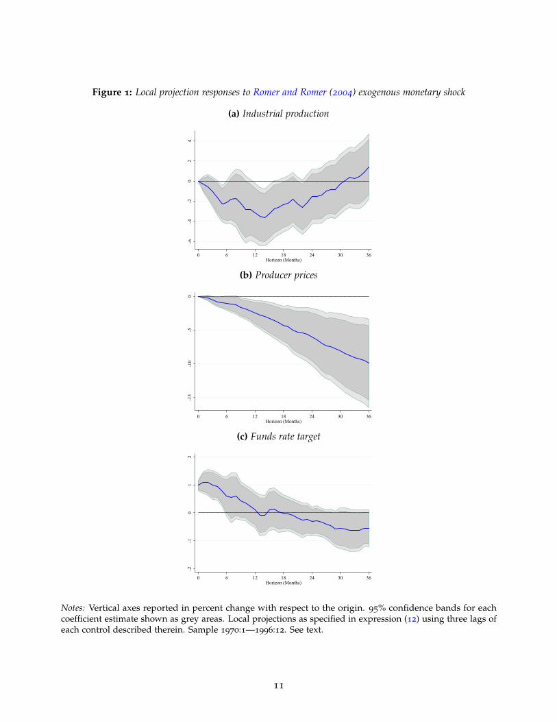
Figure 1: Local projection responses to Romer and Romer (2004) exogenous monetary shock

(a) Industrial production

-6-4

-20

24

0 6 12 18 24 30 36Horizon (Months)

(b) Producer prices

-15

-10

-50

0 6 12 18 24 30 36Horizon (Months)

(c) Funds rate target

-2-1

01

2

0 6 12 18 24 30 36Horizon (Months)

Notes: Vertical axes reported in percent change with respect to the origin. 95% confidence bands for eachcoefficient estimate shown as grey areas. Local projections as specified in expression (12) using three lags ofeach control described therein. Sample 1970:1—1996:12. See text.

11

positive response for the first four months, our response is negative right after impact. It bottoms

out at around 3.8% (rather than 4.3%) and gradually returns to zero before the end of the third year.

RR found that the response remains negative throughout the four years that they displayed.

The response of producer prices also matches well Figure 4 in RR. Panel (b) of Figure 1 shows

that prices decline on impact almost linearly for the entire period. In contrast, RR find essentially no

response in the first 2 years but then prices decline at about the same rate as they do for us. The

response of the funds rate target, although not reported in RR, is consistent with responses reported

in the literature (e.g. Christiano et al., 1999; Ramey, 2016).

4.2. Bias correction from composition effects

In this section we investigate composition effects (the balance condition in randomized controlled

trials) using the same specification used to generate the impulse responses in Figure 1. If the

RR shocks truly reflect exogenous interventions, the “treated” and “control” subpopulations of

the explanatory variables should be the same. At a fundamental level, differences will emerge

if identification has not been achieved. In that case treatment assignment is predictable by the

explanatory variables. At a more practical level, identification may hold in large samples, but in

small samples small differences between the subpopulations may remain. These small differences

are not enough to argue against identification in a statistical sense, but they will bias estimates of

the impulse response.

A simple way to explore any potential biases from composition effects using a standard local

projection is to examine the difference in means between the treatment and control subpopulations,

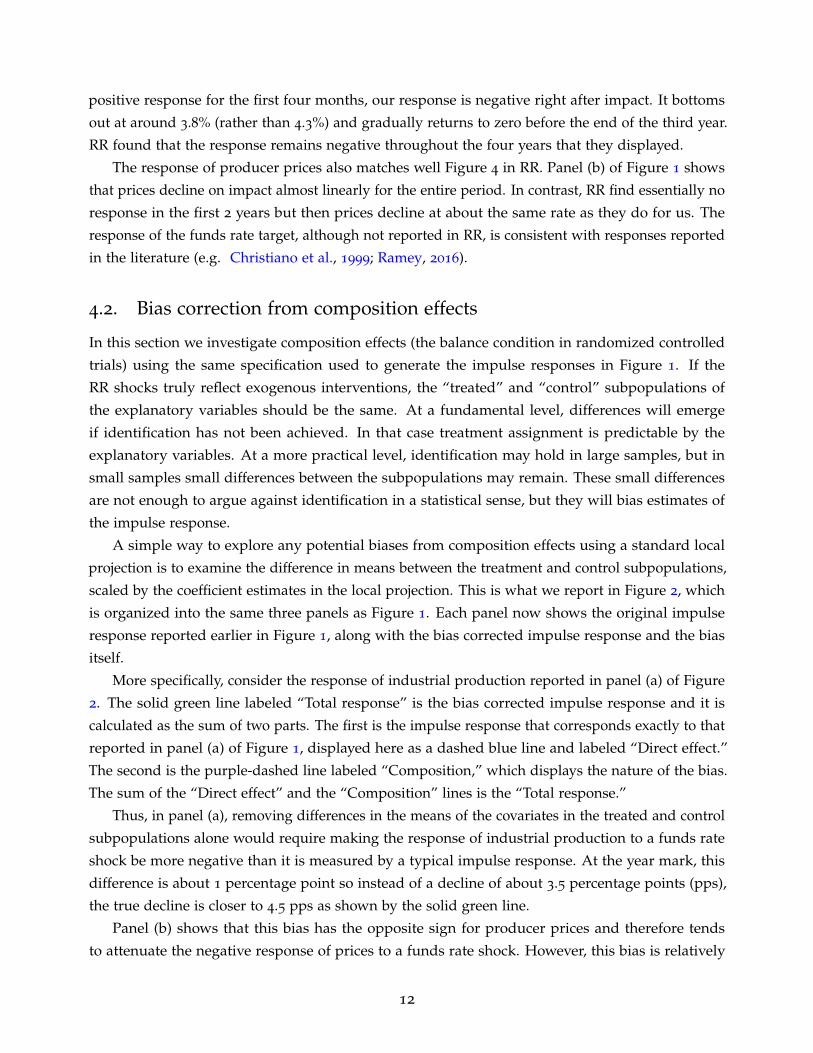
scaled by the coefficient estimates in the local projection. This is what we report in Figure 2, which

is organized into the same three panels as Figure 1. Each panel now shows the original impulse

response reported earlier in Figure 1, along with the bias corrected impulse response and the bias

itself.

More specifically, consider the response of industrial production reported in panel (a) of Figure

2. The solid green line labeled “Total response” is the bias corrected impulse response and it is

calculated as the sum of two parts. The first is the impulse response that corresponds exactly to that

reported in panel (a) of Figure 1, displayed here as a dashed blue line and labeled “Direct effect.”

The second is the purple-dashed line labeled “Composition,” which displays the nature of the bias.

The sum of the “Direct effect” and the “Composition” lines is the “Total response.”

Thus, in panel (a), removing differences in the means of the covariates in the treated and control

subpopulations alone would require making the response of industrial production to a funds rate

shock be more negative than it is measured by a typical impulse response. At the year mark, this

difference is about 1 percentage point so instead of a decline of about 3.5 percentage points (pps),

the true decline is closer to 4.5 pps as shown by the solid green line.

Panel (b) shows that this bias has the opposite sign for producer prices and therefore tends

to attenuate the negative response of prices to a funds rate shock. However, this bias is relatively

12

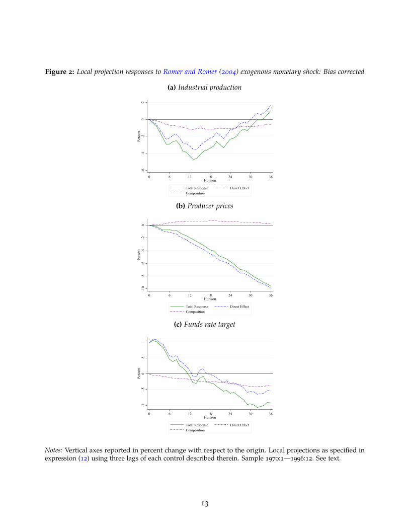
Figure 2: Local projection responses to Romer and Romer (2004) exogenous monetary shock: Bias corrected


-6-4

-20

2Pe

rcen

t

0 6 12 18 24 30 36Horizon

Total Response Direct EffectComposition

(b) Producer prices

-10

-8-6

-4-2

0Pe

rcen

t

0 6 12 18 24 30 36Horizon



-1-.5

0.5

1Pe

rcen

t

0 6 12 18 24 30 36Horizon


Notes: Vertical axes reported in percent change with respect to the origin. Local projections as specified inexpression (12) using three lags of each control described therein. Sample 1970:1—1996:12. See text.

13

small—about 0.5 pp at the year mark. The bias correction is also rather small for the funds rate,

which is consistent with the RR shock being pretty close to being exogenous—about 25bps at the

year mark.

In summary, evidence of a violation of the balance condition is scant. The more noticeable

bias happens for the response for industrial production but even then, the main conclusions in RR

remain largely intact. That said, a correction of such biases is very simple to implement as Figure 2

shows.

4.3. Direct, indirect and composition effects

Now that we have established that our local projection-based responses match RR well—although

even in this simple setting small sample biases can arise from composition effects—we show how

the methods introduced earlier can be used to further decompose each response into its constituent

elements: direct, indirect and composition effects. That is, we extend the results presented in Figure

2 using expression (8) and construct the terms delineated in expression (7). The result is displayed

in Figure 3.

The three panels of Figure 3 are organized the same way as the three panels of Figures 1 and 2.

Within each panel, we report four lines. The solid green line roughly corresponds to the response

reported in Figure 1 and is the sum of the direct (the dashed blue line), indirect (the dashed orange

line) and the composition (the dashed purple line) responses. Small differences are visible due to

the richer specification.

Consider the response of industrial production reported in panel (a) of Figure 3. The total

response largely duplicates that reported in panel (a) of Figure 1 even though it is calculated with the

richer specification described in expression (8). The shape and even the magnitudes are qualitative

and quantitatively very similar. Much like panel (a) in Figure 2, there is some bias coming from the

composition effect, but essentially no correction is needed due to the indirect effect.

As we will show later, this does not mean that there are no indirect effects—quite the contrary.

Recall that in expression (7), the indirect is obtained by comparing the mean of the covariates in the

treated subpopulation relative to the overall mean, scaled by estimates of their slope coefficients. In

a well balanced experiment (such as this one), that difference will be nearly zero at the mean so no

matter the scaling, the indirect effect evaluated at the sample mean is usually close to zero. However,

whether or not the indirect effect matters depends on the slope coefficient estimates themselves.

These are significantly different from zero and give rise to interesting state-dependent effects, as we

illustrate in the next section.

In sum, removing the indirect and composition effects leaves a more amplified response of

industrial production (by about one percentage point more) than reported earlier. Indirect and

composition effect corrections for prices and the funds rate target—reported in panels (b) and (c)

of Figure 3—are much smaller, in the order of one half of a percentage point or less and generally

induce responses that don’t differ materially from those originally reported in Figure 1.

14

Figure 3: Local projection responses to exogenous RR monetary shock: Blinder-Oaxaca decomposition


-5-4

-3-2

-10

Perc

ent

0 6 12 18 24 30 36Horizon

Total Response Direct EffectIndirect Effect Composition

(b) Producer prices

-15

-10

-50

Perc

ent

0 6 12 18 24 30 36Horizon



-2-1

01

2Pe

rcen

t

0 6 12 18 24 30 36Horizon



15

5. State-dependence: historical episodes revisited

In this section we illustrate how the Blinder-Oaxaca decomposition can be used to explore historical

episodes. In particular, we will revisit expressions (9) and (10) using the same data and examples

we used in the previous section. We focus on two particular episodes: November 1987 and February

1996. In October 19, 1987 the stock market crashed, not just in the U.S. but across several markets

worldwide. By the end of October, stocks had lost about 23% of their value. The Federal Reserve

responded by lowering the federal funds rate by 50 basis points. Given what the economy looked

like in October 1987, we ask whether monetary policy would have been expected to be an effective

tool in stimulating the economy.

The second episode, in contrast, is not attached to any significant event. Instead it sits ap-

proximately in the middle of a long expansion and in the middle of a period of relatively stable

interest rates. That is, there were no significant policy actions before or after. On the other hand,

the mid-1990s are often thought to coincide with a boost in productivity that would last until the

mid-2000s, right before the Great Recession. We think that the relative calm of this episode provides

a nice counterpoint to the 1987 episode.

In both episodes, given economic conditions in the lead in, the path that the federal funds rate

would have expected to follow roughly coincided with the historical average. This is important. Any

differences in the responses of prices or industrial production cannot be attributed to differences in

the expected policy path. Importantly, note that we are not rationalizing the data ex-post. Rather,

using the full sample and the data up to the date considered, we display the path of the funds rate,

producer prices and industrial output expected to prevail.

Figure 4 displays the 1987 episode on the left-hand side and the 1996 episode on the right-hand

side. The first row shows the responses of industrial production, the second row for producer prices

and the third row for the funds rate. We show as a solid line the same responses displayed earlier in

Figure 3 with a solid line as well, whereas the dashed line displays the impulse response conditional

on the particular historical episode under consideration.

Consider 1987 first, displayed in panels (a), (c), and (e). As remarked earlier, the path of the

funds rate displayed in panel (e) is nearly the same as the average path for the entire sample.

Any differences appear at the very end of the horizon displayed. However, this is also when the

coefficients are least precisely estimated. At a minimum, it can be said without fear of exaggeration

that for the first two years, the funds rate paths are nearly identical. Are these paths therefore

associated with similar responses in industrial production and producer prices?

Panel (a) in Figure 4 clear shows this not to be the case. Even if we focus primarily on the

first two years, the response of industrial production conditional on the outlook in October 1987

is considerably more muted. Note that all along we have assumed the responses to be symmetric.

That is, we have implicitly restricted the specification so that an increase in the funds rate generates

the same response (but with the opposite sign) on industrial production and producer prices.

Thus, a surprise reduction in the funds rate in November 1987 would have been expected to

16

Figure 4: Local projection responses to exogenous RR monetary shock: Historical Episodes

Industrial production

(a) November 1987

-6-4

-20

Perc

ent

0 6 12 18 24 30 36Horizon

Total Response: baseline Total response starting in 1987m11

(b) February 1996

-8-6

-4-2

0Pe

rcen

t

0 6 12 18 24 30 36Horizon


Producer prices

(c) November 1987

-8-6

-4-2

0Pe

rcen

t

0 6 12 18 24 30 36Horizon


(d) February 1996-8

-6-4

-20

2Pe

rcen

t

0 6 12 18 24 30 36Horizon


Federal funds rate

(e) November 1987

-4-3

-2-1

01

Perc

ent

0 6 12 18 24 30 36Horizon


(f) February 1996

-3-2

-10

12

Perc

ent

0 6 12 18 24 30 36Horizon


Notes: Vertical axes reported in percent change with respect to the origin. Local projections as specified inexpression (8) using three lags of each control described therein and then evaluated with data up to October1987 in columns (a), (c), and (e); and January 1996 in columns (b), (d), and (f) . Sample 1970:1—1996:12. Seetext.

17

stimulate industrial production by a much smaller amount (at the 2-year mark the difference is

about 2-percentage points) than would have been the case historically.

Initially, producer prices would have reacted somewhat more strongly than the average although

the differences are small throughout and by the two-year mark, the cumulative change in prices

would have been nearly identical. Altogether these figures suggest that the Federal Reserve faced a

more unfavorable trade-off in terms of economic activity versus inflation, than had been the case

historically in our sample.

Turning to the 1996 episode, matters are quite different. Again, panel (f) of Figure 4 shows

that the funds rate responses are quite similar. In fact, if anything, the funds rate path would have

been expected to be slightly steeper initially. In contrast to the 1987 industrial production response

displayed in panel (a) fo the same figure, the 1996 response reported in panel (b) is nearly identical

to the historical average. The only difference emerges with producer prices, as panel (d) makes clear.

The response of prices is much more muted. By the 2-year mark, producer prices are essentially

unchanged and only start declining thereafter.

It is an interesting juxtaposition, in both episodes we find a more unfavorable economic activity-

inflation trade-off. In 1987 this is largely due to the much more muted response of industrial

production relative to the historical average. In 1996 industrial production behaves no differently

than on average, but the price response becomes significantly more muted.

6. Monetary policy asymmetries

Up to this point we have shown that with a trivial extension of the local projections framework, we

gain much more clarity on how to interpret impulse responses used by a vast literature before us.

We have seen how composition effects can crop up and attenuate or amplify an impulse response.

Moreover, such composition effects provide for a natural way to evaluate identification. If the

experiments are well designed and properly identified, there should be no composition effects.

The second latent element of a typical impulse response is the indirect effect, which may exist

even in a properly identified setting. On average the indirect effect may appear to be small but

as we have seen, there can be considerable differences lurking in the sample when one examines

alternative historical episodes.

In this section we revisit the issue of symmetry, that is, the notion that an increase in the funds

rate has the same effect (but with the opposite sign) than a decrease. Several authors before us have

found evidence that this is the case, e.g. Angrist et al. (2016) and Tenreyro and Thwaites (2016).

Here we show that a simple modification of our framework delivers the necessary tools to assess

this symmetry hypothesis.

Return to expression (8), repeated here for convenience:


0 + δt βh + δt(xt − x)θh + ωt+h; h = 0, 1, . . . , H; t = h, ..., T.

18

Now instead of two subpopulations, the control and treated subpopulations (the latter scaled

by the dose δt), we consider three. The control subpopulation stays the same, but the treated

subpopulation gets divided into rate increases and rate decreases. We denote quantities for the

treated subpopulation when the treatment consists in raising the funds rate using the subscript ∆,

and we use the subscript ∇ when considering decreasing the funds rate instead. This extension

poses no difficulty since we can recast expression (8) as:

yt+h =µh0 + (xt − x)γh

0+ (13)

δ∆t βh

∆ + δ∇t βh∇+

δ∆t (xt − x)θh

∆+

δ∇t (xt − x)θh∇ + ωt+h; h = 0, 1, . . . , H; t = h, ..., T.

where δ∆ is the change in the policy rate if that change is positive, and is zero otherwise; and δ∇ is

symmetrically defined.

Estimates of expression (13) can then be used to construct an extension of the Blinder-Oaxaca

decomposition, similarly to expression (7), that is:

Direct effect of increases: βh∆

decreases: βh∇

Indirect effect of increases: (x∆ − x)θh∆

decreases: (x∇ − x)θh∇

Composition effect increases: (x∆ − x0)γh0

decreases: (x∇ − x0)γh0

(14)

As an illustration, Figure 5 provides impulse responses obtained by these methods when one

stratifies the RR shocks into negative and positive shocks. Notice that, for example, if the experiment

is well identified, an exogenous negative shock (a funds rate cut) during a recession is just as likely

as a negative shock in the middle of an expansion. This observation is worth keeping in mind as we

comment on our findings.

Note that both columns in Figure 5 report responses to the same experiment, meaning, an

exogenous one percent increase in the funds rate. The common scaling facilitates the discussion.

The results in Figure 5 may seem to contradict what has been reported in the literature at first blush.

Negative RR shocks (reported on the left-hand column) appear to carry more of a bang: industrial

production and prices respond by larger amounts relative to when there is a positive RR shock

(reported on the right-hand column). Importantly, these differences do not crop up because the path

of the funds rate is such that interest rates are kept higher for longer. On the contrary, as panel (c)

of the figure make evident.

19

Figure 5: Local projection responses to exogenous RR monetary shock: Historical Episodes


Negative RR shock

-15

-10

-50

5Pe

rcen

t

0 6 12 18 24 30 36Horizon

Total Response (Cuts) Direct Effect (Cuts)Indirect Effect (Cuts) Composition (Cuts)

Positive RR shock

-4-2

02

46

Perc

ent

0 6 12 18 24 30 36Horizon

Total Response (Increases) Direct Effect (Increases)Indirect Effect (Increases) Composition (Increases)

(b) Producer prices

-20

-15

-10

-50

Perc

ent

0 6 12 18 24 30 36Horizon


-6-4

-20

2Pe

rcen

t

0 6 12 18 24 30 36Horizon


(c) Federal funds rate

-4-3

-2-1

01

Perc

ent

0 6 12 18 24 30 36Horizon


-10

12

Perc

ent

0 6 12 18 24 30 36Horizon



20

What makes the figure tricky to interpret is that we have no context to evaluate under what

conditions an exogenous cut in interest rates takes place (or for that matter, an increase). This is

where the allowance for state-dependence through the indirect effect terms in expression (14) will

come in handy. First, notice that periods of expansion are more abundant than periods of recession.

Thus a larger fraction of the sample for which an exogenous RR shock is observed take place in

periods of expansion. In those periods, a cut in rates is likely to overstimulate the economy relative

to other times.

In contrast, positive shocks (meaning increases in the funds rate) are also more likely to be

observed in periods of expansion. But those are the periods where one expects that the funds rate

will be endogenously increased and therefore may appear to have a lesser effect in that context.

Alas, the extra terms in the decomposition allow us to examine more closely for asymmetries

during particular episodes that may make more economic sense from the point of view of a particular

experiment. That is, consider negative RR shocks during periods of recession when interest rates

are generally reduced or examine positive RR shocks during expansions when interest rates are

generally increased.

7. Conclusion

Current thinking about impulse responses and their role in monetary economics has been greatly

influenced by the tight link between vector autoregressions (or VARs) and the solutions to traditional

linear or linearized models of monetary economies. These solutions tend to be of first order.

Extending the lag length of the VAR was the natural first step toward generalizing the empirical

analysis away from the necessary strictures of theory. Sims (1980) made that much clear in his

seminal paper. The literature has made great strides since within this framework.

Rather than starting from the theory and moving toward the empirics, this paper moves in the

opposite direction. It starts by taking the impulse response as a legitimate moment of interest, akin

to a dynamic average treatment effect. And in doing so, it borrows the econometric tools from an

extensive literature in applied microeconomics. Our contribution is thus to show the ways in which

VARs impose constraints on impulse responses that are not supported by the data. By taking a less

structural approach to the data generating process, we have shown simple ways in which to exploit

the information in the sample that inform about the manner monetary economies work.

Local projections (Jorda, 2005) have facilitated the combination of the methods available in

applied microeconomics and shown how they can help in applied macroeconomics. For example, we

have shown that even when there is proper identification, small sample differences in the treated and

control subpopulations of the explanatory variables can generate biases in the measured impulse

response. We called these biases the composition effect.

Moreover, we have shown policy interventions can affect the manner explanatory variables

affect outcomes, even when on average this effect is zero. The implication is that the same policy

intervention will be expected to have a different effect depending on the conditions under which the

21

intervention is effected. We called this the indirect effect. Using this result, we have shown how

different historical episodes can be brought to bear on the monetary policy trade-offs a policymaker

could face in practice depending on the state of the economy.

These are some of the preliminary but important results that we have uncovered by using

relatively straightforward regression methods. Of course, several extensions of this framework

are possible and we have highlighted some of them in the text. Our hope is that the methods we

propose will be seen as complementary to existing methods and a useful building block for future

research.

22

References

Angrist, J. D., O. Jorda, and G. M. Kuersteiner (2016). Semiparametric estimates of mon-etary policy effects: String theory revisited. Journal of Business and Economic Statis-tics http://dx.doi.org/10.1080/07350015.2016.1204919.

Blinder, A. S. (1973). Wage discrimination: Reduced form and structural estimates. The Journal ofHuman Resources 8(4), 436–455.

Christiano, L. J., M. Eichenbaum, and C. L. Evans (1999). Monetary policy shocks: What have welearned and to what end? In J. B. Taylor and M. Woodford (Eds.), Handbook of Macroeconomics,Volume 1 of Handbook of Macroeconomics, Chapter 2, pp. 65–148. Elsevier.

Cloyne, J. and P. Hurtgen (2016, October). The Macroeconomic Effects of Monetary Policy: A NewMeasure for the United Kingdom. American Economic Journal: Macroeconomics 8(4), 75–102.

Fortin, N., T. Lemieux, and S. Firpo (2011). Decomposition Methods in Economics, Volume 4 of Handbookof Labor Economics, Chapter 1, pp. 1–102. Elsevier.

Gertler, M. and P. Karadi (2015, January). Monetary Policy Surprises, Credit Costs, and EconomicActivity. American Economic Journal: Macroeconomics 7(1), 44–76.

Gurkaynak, R. S., B. Sack, and E. Swanson (2005, May). Do Actions Speak Louder Than Words?The Response of Asset Prices to Monetary Policy Actions and Statements. International Journal ofCentral Banking 1(1).

Jorda, O. (2005, March). Estimation and Inference of Impulse Responses by Local Projections.American Economic Review 95(1), 161–182.

Jorda, O., M. Schularick, and A. M. Taylor (2017, January). Large and State-Dependent Effects ofQuasi-Random Monetary Experiments. Working Paper Series 2017-2, Federal Reserve Bank ofSan Francisco.

Miranda-Agrippino, S. (2015, June). Unsurprising Shocks: Information, Premia, and the MonetaryTransmission. Discussion Papers 1613, Centre for Macroeconomics (CFM).

Oaxaca, R. (1973, October). Male-Female Wage Differentials in Urban Labor Markets. InternationalEconomic Review 14(3), 693–709.

Ramey, V. A. (2016). Macroeconomic shocks and their propagation. In J. B. Taylor and H. Uhlig(Eds.), Handbook of Macroeconomics, Volume 2A, pp. 71–162. Elsevier.

Romer, C. D. and D. H. Romer (2004, September). A New Measure of Monetary Shocks: Derivationand Implications. American Economic Review 94(4), 1055–1084.

Rubin, D. B. (1974). Estimating causal effects of treatments in randomized and nonrandomizedstudies. Journal of Educational Psychology 66(5), 688–701.

Sims, C. A. (1980). Macroeoconomics and reality. Econometrica 48(1), 1–48.

Tenreyro, S. and G. Thwaites (2016, October). Pushing on a String: US Monetary Policy Is LessPowerful in Recessions. American Economic Journal: Macroeconomics 8(4), 43–74.

Wooldridge, J. M. (2001, July). Econometric Analysis of Cross Section and Panel Data, Volume 1 of MITPress Books. The MIT Press.

23

Documents

Direct, indirect, and composition effects of monetary