Embed Size (px)
Citation preview
Direct Imaging of Exoplanets
I. Techniques
a) Adaptive Optics
b) Coronographs
c) Differential Imaging
d) Nulling Interferometers
e) External Occulters
II. Results
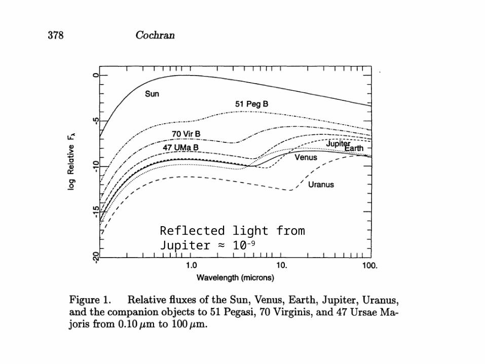
Reflected light from Jupiter ≈ 10–9
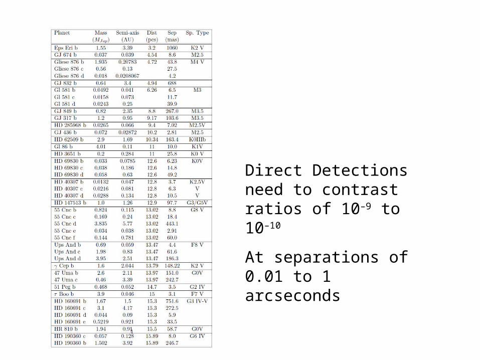
Direct Detections need to contrast ratios of 10–9 to 10–10
At separations of 0.01 to 1 arcseconds
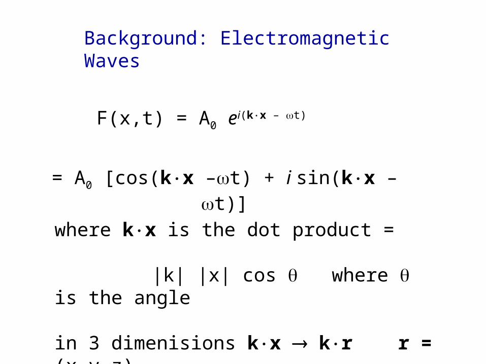
Background: Electromagnetic Waves
F(x,t) = A0 ei(kx – t)
= A0 [cos(kx –t) + i sin(kx –t)]
where kx is the dot product =
|k| |x| cos where is the angle
in 3 dimenisions kx kr r = (x,y,z)
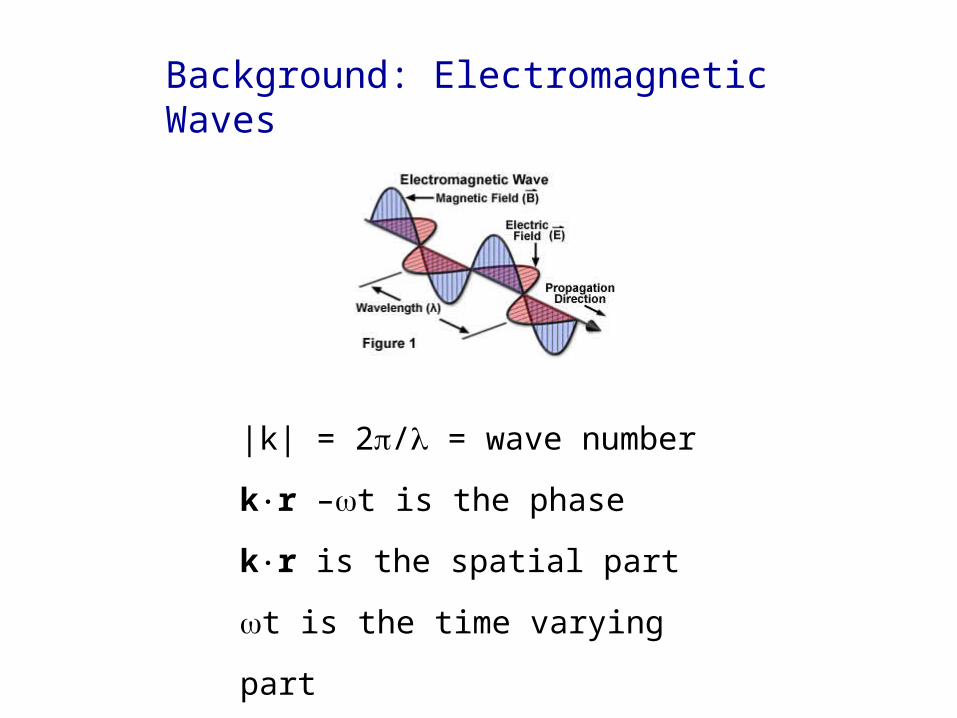
Background: Electromagnetic Waves
|k| = 2/ = wave number
kr –t is the phase
kr is the spatial part
t is the time varying part
Background: Fourier Transforms
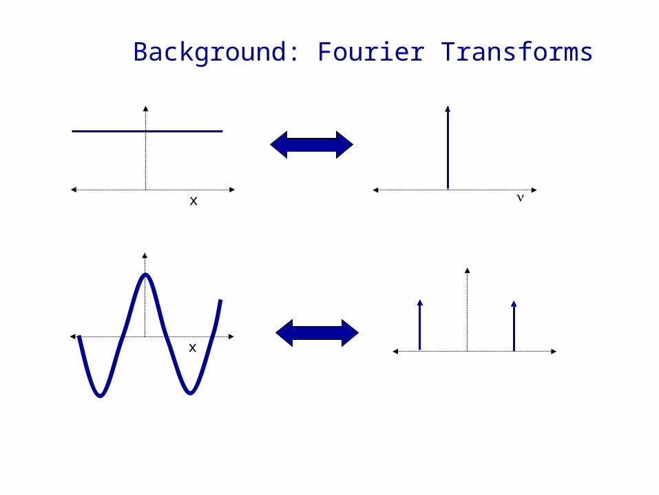
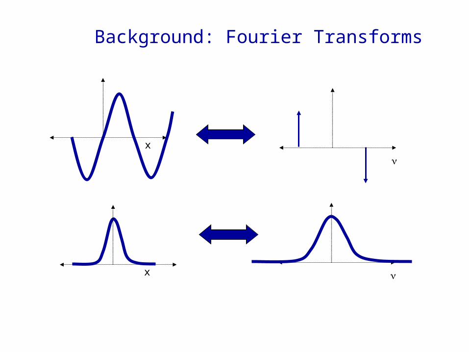
Cosines and sines represent a set of orthogonal functions.
Meaning: Every continuous function can be represented by a sum of trigonometric terms
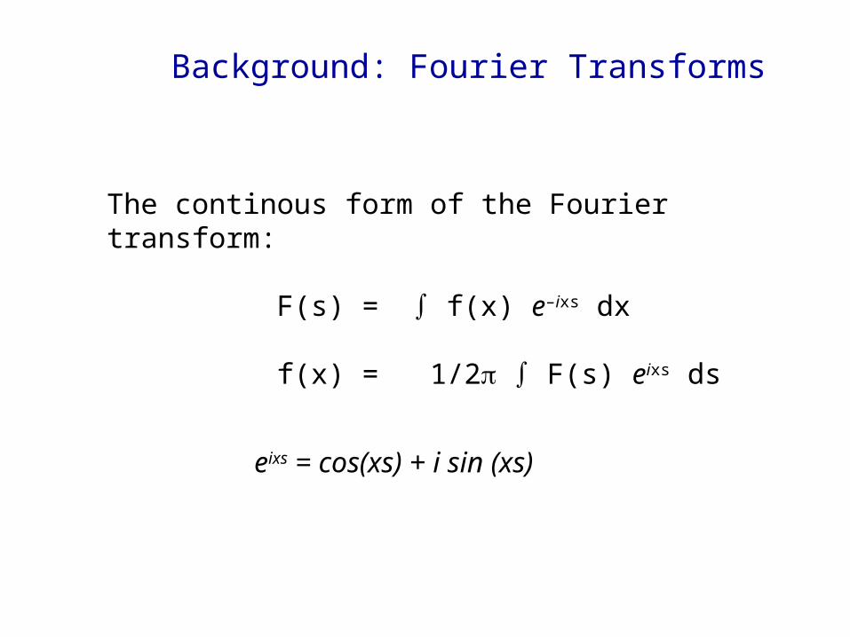
Background: Fourier Transforms
The continous form of the Fourier transform:
F(s) = f(x) e–ixs dx
f(x) = 1/2 F(s) eixs ds
eixs = cos(xs) + i sin (xs)
Background: Fourier Transforms
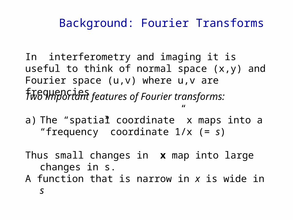
In interferometry and imaging it is useful to think of normal space (x,y) and Fourier space (u,v) where u,v are frequencies
Two important features of Fourier transforms:
a) The “spatial coordinate” x maps into a “frequency” coordinate 1/x (= s)
Thus small changes in x map into large changes in s. A function that is narrow in x is wide in s
Background: Fourier Transforms
x
x
Background: Fourier Transforms
x
x
Background: Fourier Transforms
x
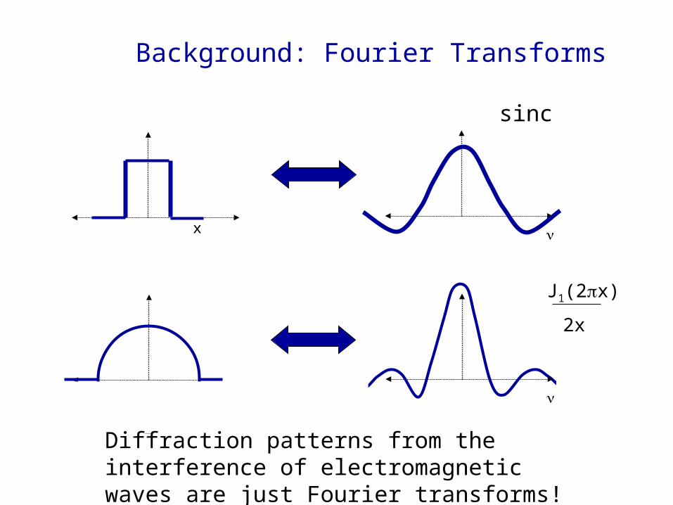
sinc
x
J1(2x)
2x
Diffraction patterns from the interference of electromagnetic waves are just Fourier transforms!
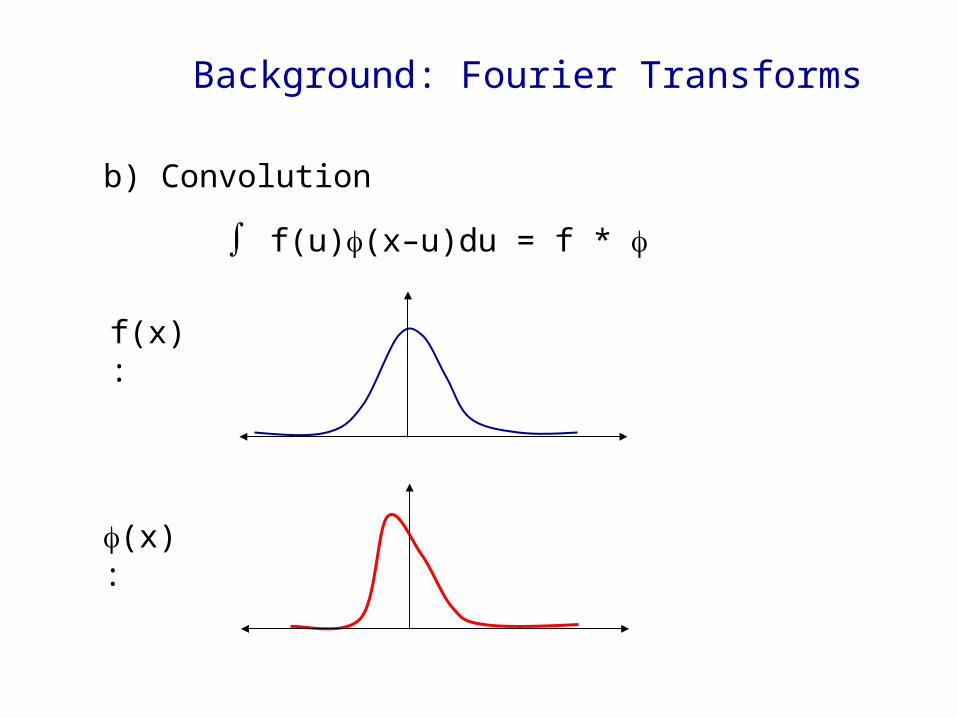
b) Convolution
Background: Fourier Transforms
f(u)(x–u)du = f *
f(x):
(x):
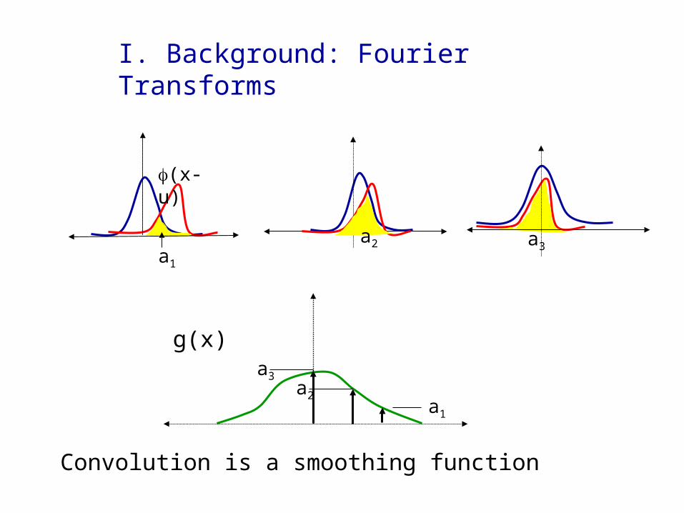
I. Background: Fourier Transforms
(x-u)
a1
a2
g(x)a3
a2
a3
a1
Convolution is a smoothing function
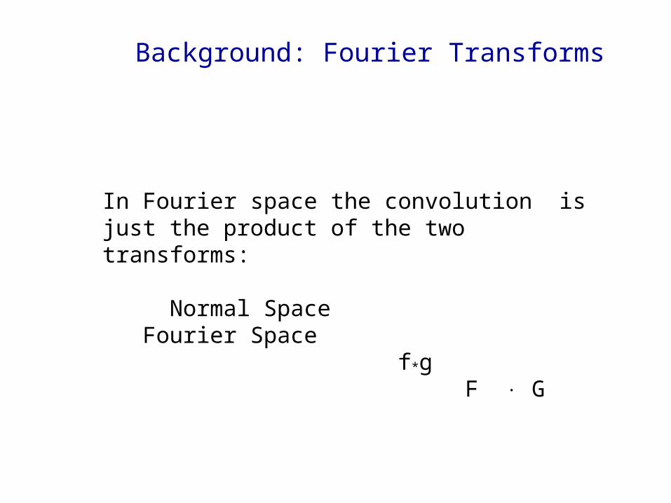
In Fourier space the convolution is just the product of the two transforms:
Normal Space Fourier Space f*g F G
Background: Fourier Transforms
Example of an Adaptive Optics System: The Eye-Brain
The brain interprets an image, determines its correction, and applies the correction either voluntarily of involuntarily
Lens compression: Focus corrected mode
Tracking an Object: Tilt mode optics system
Iris opening and closing to intensity levels: Intensity control mode
Eyes squinting: An aperture stop, spatial filter, and phase controlling mechanism
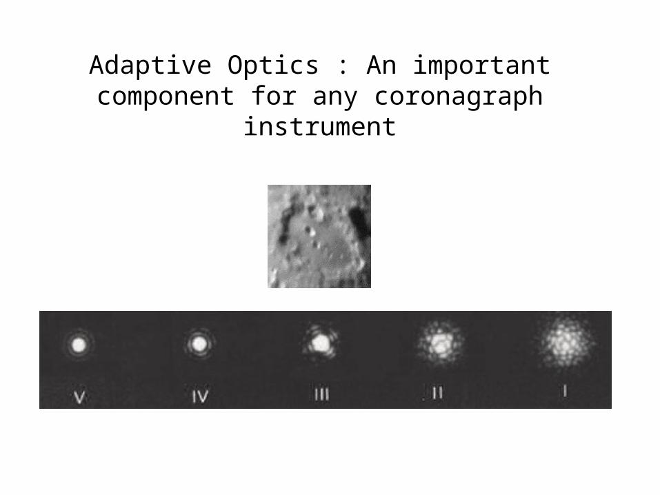
Adaptive Optics : An important component for any coronagraph instrument
Adaptive Optics
The scientific and engineering discipline whereby the performance of an optical signal is improved by using information about the environment through which it passes
AO Deals with the control of light in a real time closed loop and is a subset of active optics.
Adaptive Optics: Systems operating below 1/10 Hz
Active Optics: Systems operating above 1/10 Hz
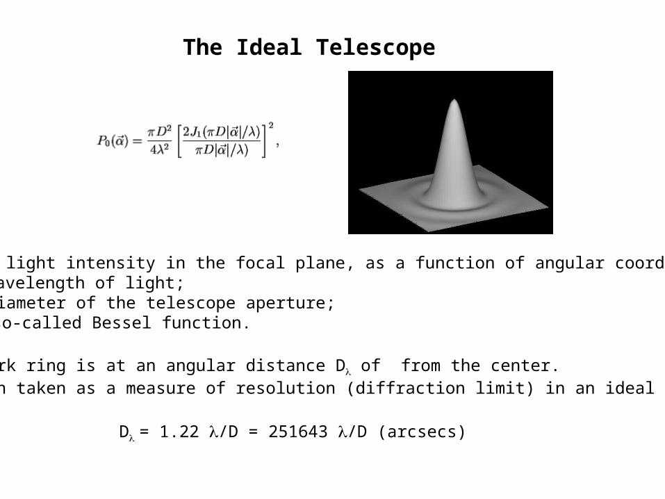
where: • P() is the light intensity in the focal plane, as a function of angular coordinates ; • is the wavelength of light; • D is the diameter of the telescope aperture; • J1 is the so-called Bessel function.
The first dark ring is at an angular distance D of from the center.This is often taken as a measure of resolution (diffraction limit) in an ideal telescope.
The Ideal Telescope
D= 1.22 /D = 251643 /D (arcsecs)
Telescope
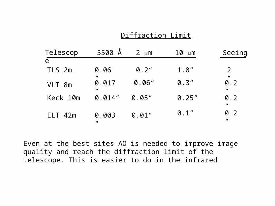
Diffraction Limit
5500 Å 2 m 10 m
TLS 2m
VLT 8m
Keck 10m
ELT 42m
0.06“ 0.2“ 1.0“
0.017“
0.014“
0.003“
0.06“
0.05“
0.01“
0.3“
0.25“
0.1“
Seeing
2“
0.2“
0.2“
0.2“
Even at the best sites AO is needed to improve image quality and reach the diffraction limit of the telescope. This is easier to do in the infrared
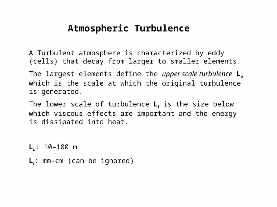
Atmospheric Turbulence
A Turbulent atmosphere is characterized by eddy (cells) that decay from larger to smaller elements.
The largest elements define the upper scale turbulence Lu which is the scale at which the original turbulence is generated.
The lower scale of turbulence Ll is the size below which viscous effects are important and the energy is dissipated into heat.
Lu: 10–100 m
Ll: mm–cm (can be ignored)
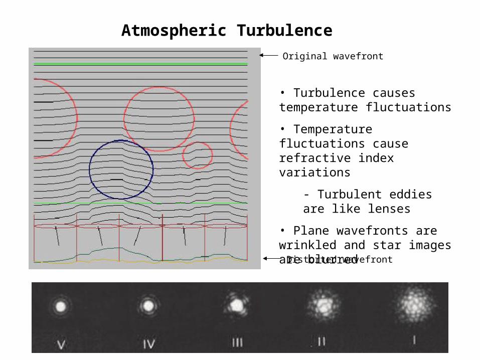
• Turbulence causes temperature fluctuations
• Temperature fluctuations cause refractive index variations
- Turbulent eddies are like lenses
• Plane wavefronts are wrinkled and star images are blurred
Atmospheric Turbulence
Original wavefront
Distorted wavefront
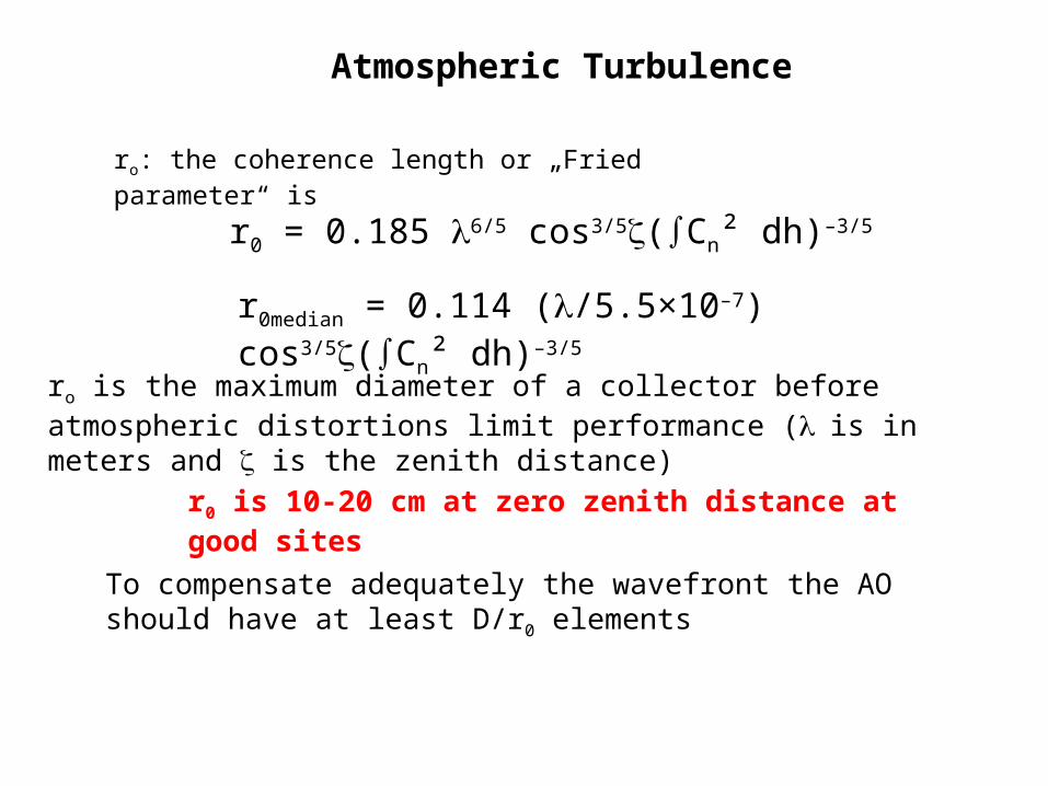
ro: the coherence length or „Fried parameter“ is
r0 = 0.185 6/5 cos3/5(∫Cn² dh)–3/5
r0median = 0.114 (/5.5×10–7) cos3/5(∫Cn² dh)–3/5
ro is the maximum diameter of a collector before atmospheric distortions limit performance (is in meters and is the zenith distance)
r0 is 10-20 cm at zero zenith distance at good sites
To compensate adequately the wavefront the AO should have at least D/r0 elements
Atmospheric Turbulence
Definitions
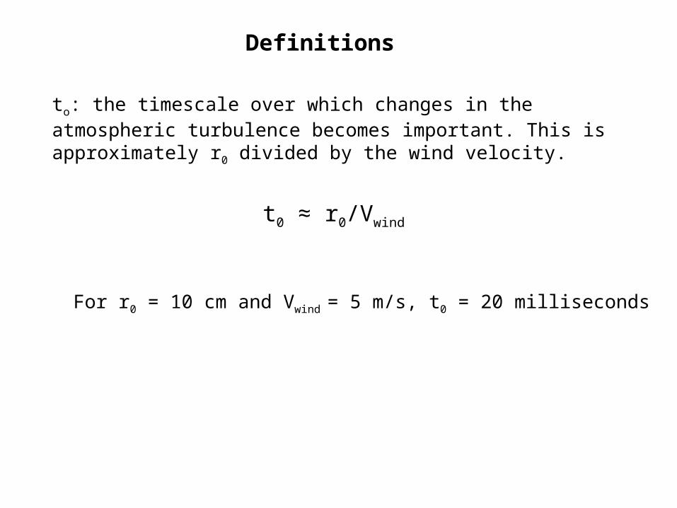
to: the timescale over which changes in the atmospheric turbulence becomes important. This is approximately r0 divided by the wind velocity.
t0 ≈ r0/Vwind
For r0 = 10 cm and Vwind = 5 m/s, t0 = 20 milliseconds
Definitions
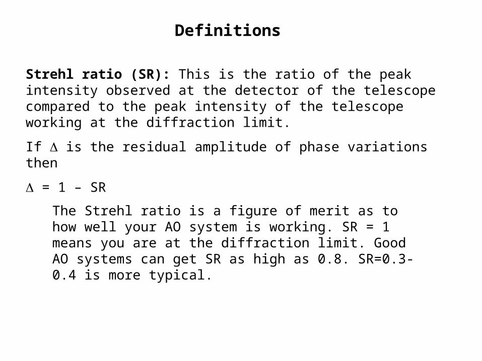
Strehl ratio (SR): This is the ratio of the peak intensity observed at the detector of the telescope compared to the peak intensity of the telescope working at the diffraction limit.
If is the residual amplitude of phase variations then
= 1 – SR
The Strehl ratio is a figure of merit as to how well your AO system is working. SR = 1 means you are at the diffraction limit. Good AO systems can get SR as high as 0.8. SR=0.3-0.4 is more typical.
Definitions
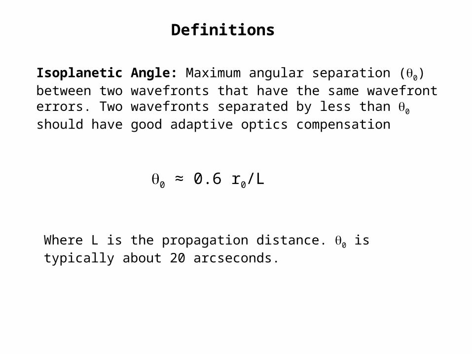
Isoplanetic Angle: Maximum angular separation (0) between two wavefronts that have the same wavefront errors. Two wavefronts separated by less than 0 should have good adaptive optics compensation
0 ≈ 0.6 r0/L
Where L is the propagation distance. 0 is typically about 20 arcseconds.
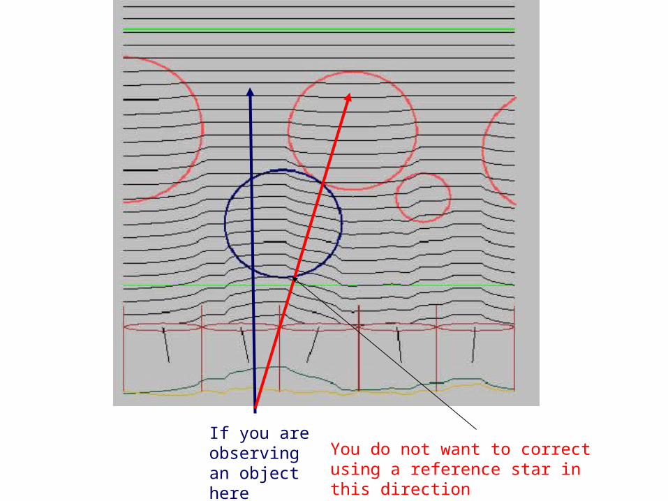
If you are observing an object here
You do not want to correct using a reference star in this direction
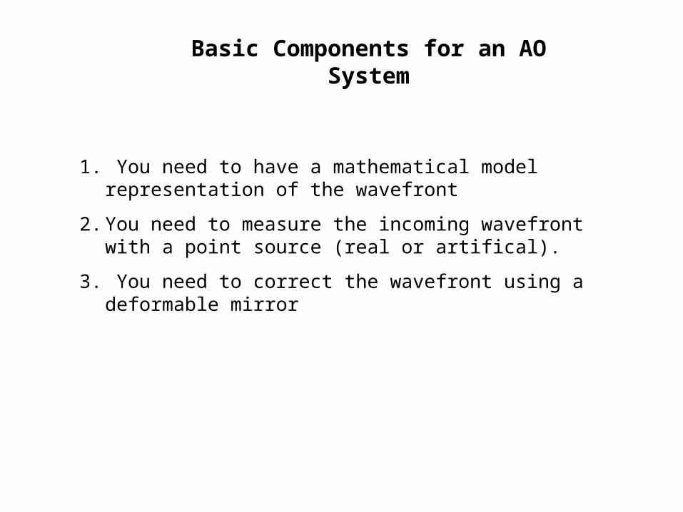
Basic Components for an AO System
1. You need to have a mathematical model representation of the wavefront
2. You need to measure the incoming wavefront with a point source (real or artifical).
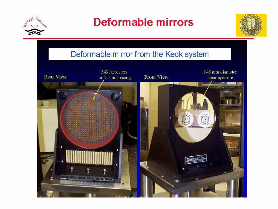
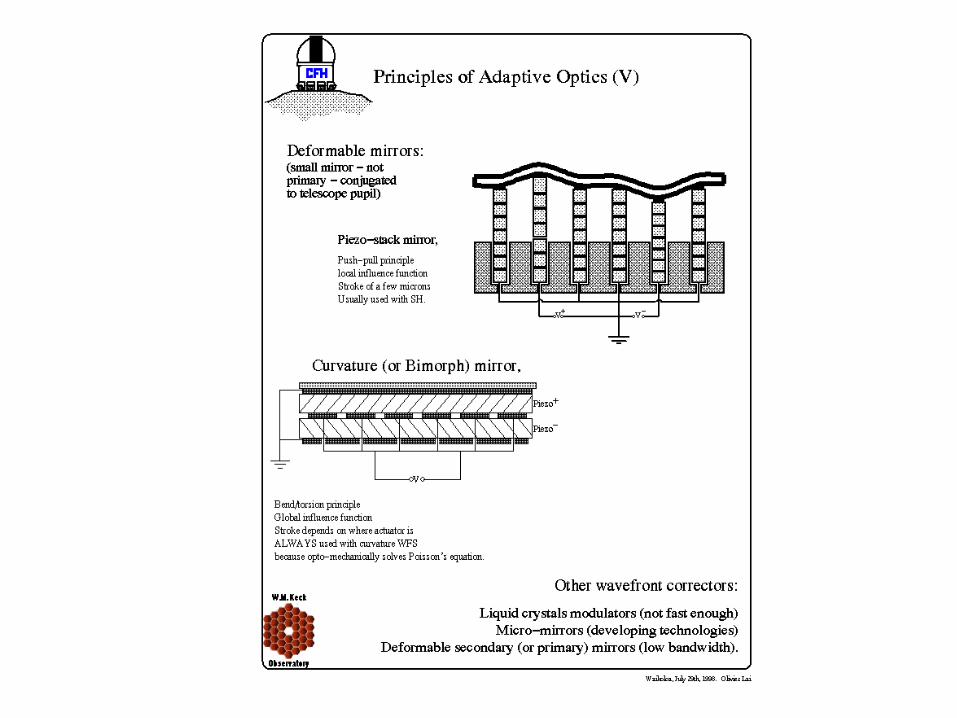
3. You need to correct the wavefront using a deformable mirror
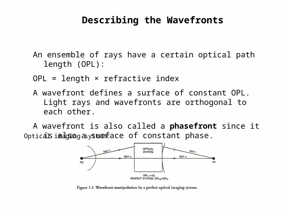
Describing the Wavefronts
An ensemble of rays have a certain optical path length (OPL):
OPL = length × refractive index
A wavefront defines a surface of constant OPL. Light rays and wavefronts are orthogonal to each other.
A wavefront is also called a phasefront since it is also a surface of constant phase.
Optical imaging system:
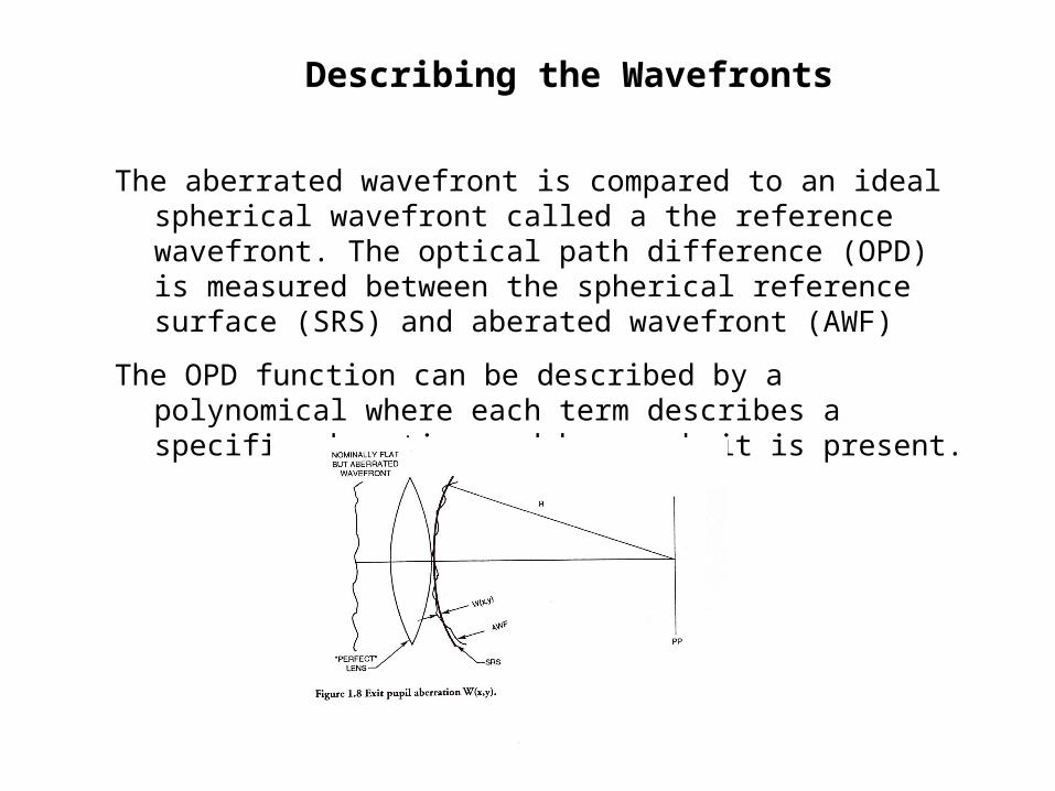
Describing the Wavefronts
The aberrated wavefront is compared to an ideal spherical wavefront called a the reference wavefront. The optical path difference (OPD) is measured between the spherical reference surface (SRS) and aberated wavefront (AWF)
The OPD function can be described by a polynomical where each term describes a specific aberation and how much it is present.
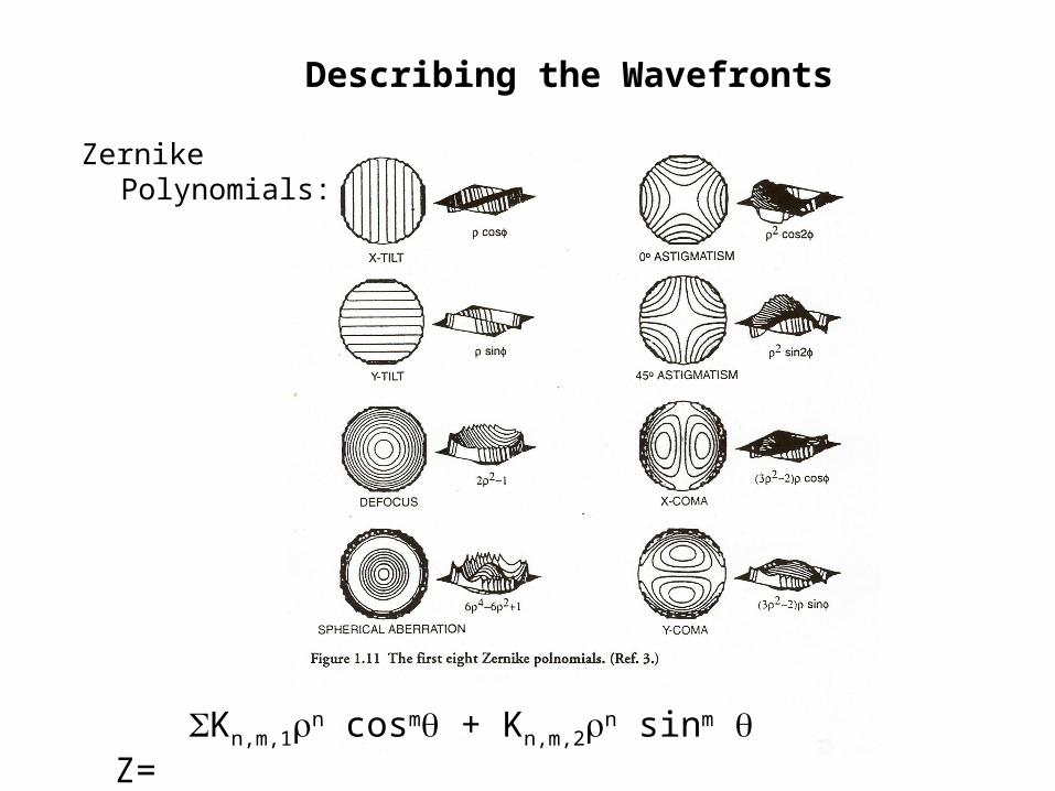
Describing the Wavefronts
Zernike Polynomials:
Z= Kn,m,1n cosm + Kn,m,2n sinm
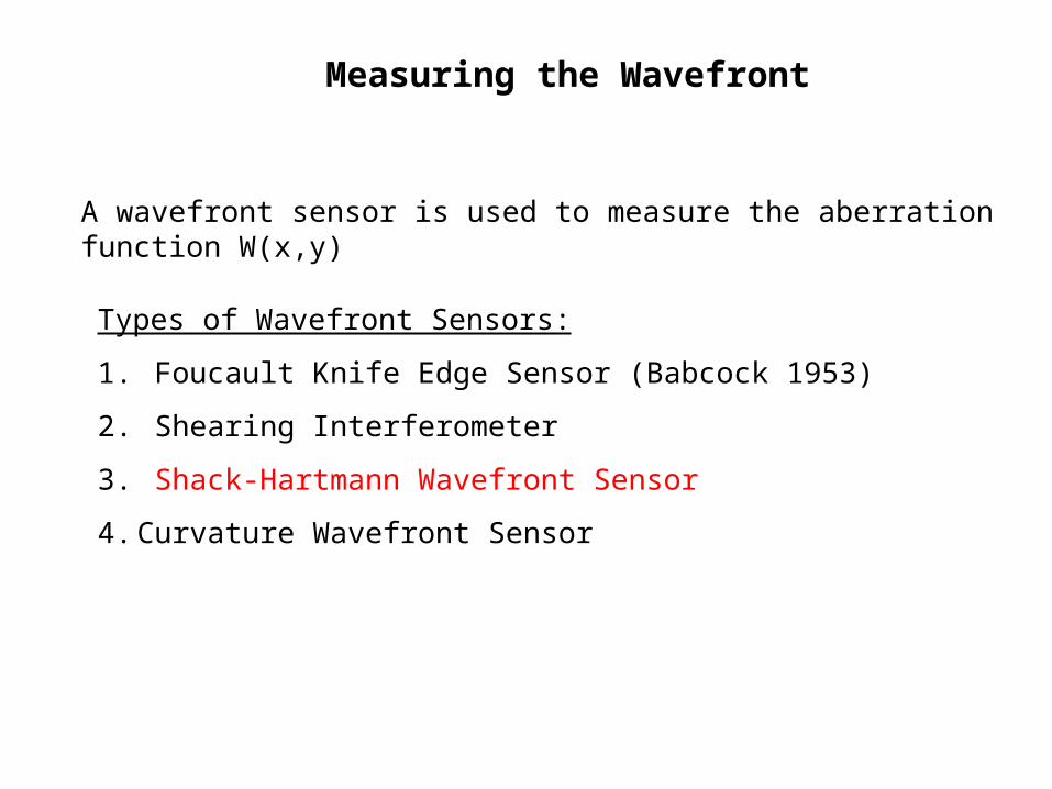
Measuring the Wavefront
A wavefront sensor is used to measure the aberration function W(x,y)
Types of Wavefront Sensors:
1. Foucault Knife Edge Sensor (Babcock 1953)
2. Shearing Interferometer
3. Shack-Hartmann Wavefront Sensor
4. Curvature Wavefront Sensor
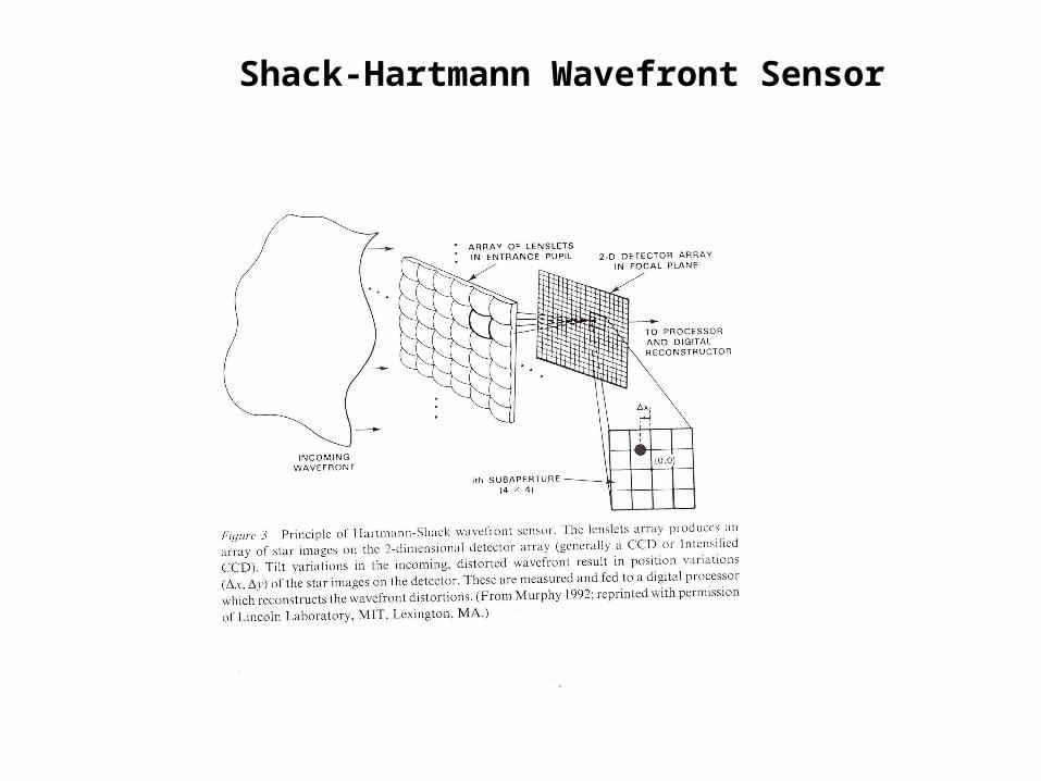
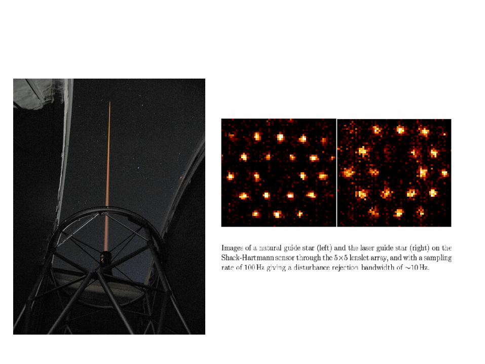
Shack-Hartmann Wavefront Sensor
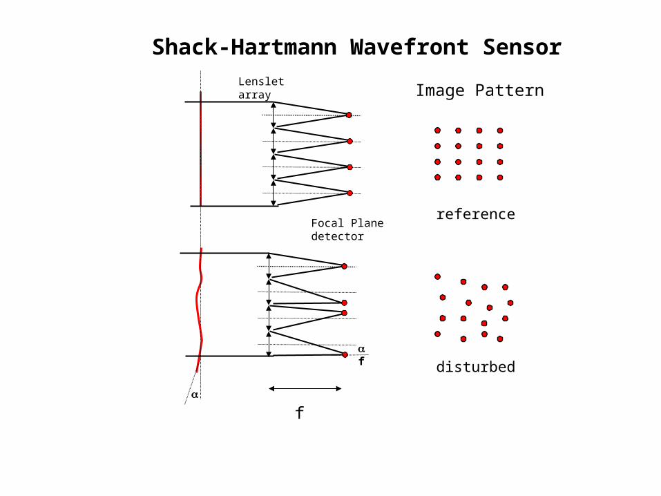
Shack-Hartmann Wavefront Sensor
f
Image Pattern
reference
disturbed
f
Lenslet array
Focal Plane detector
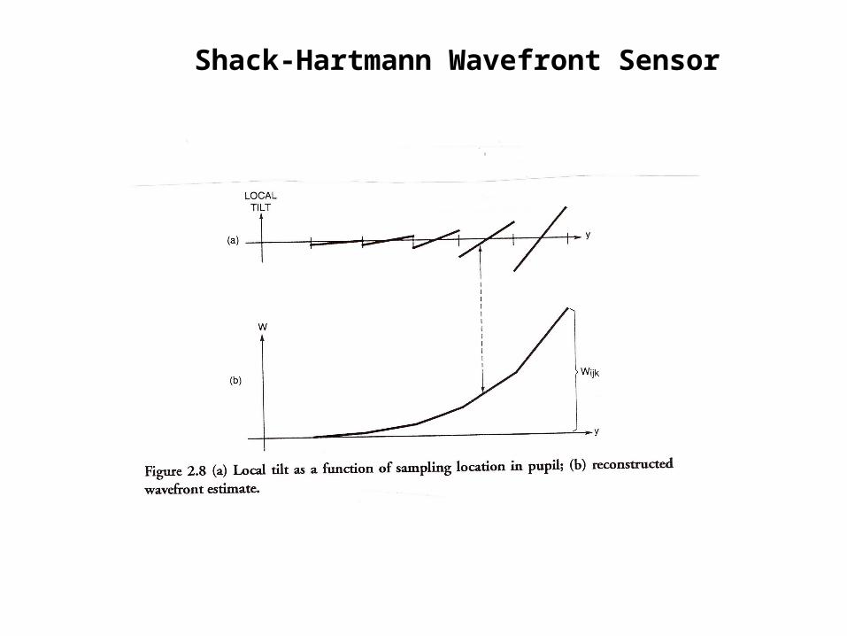
Shack-Hartmann Wavefront Sensor
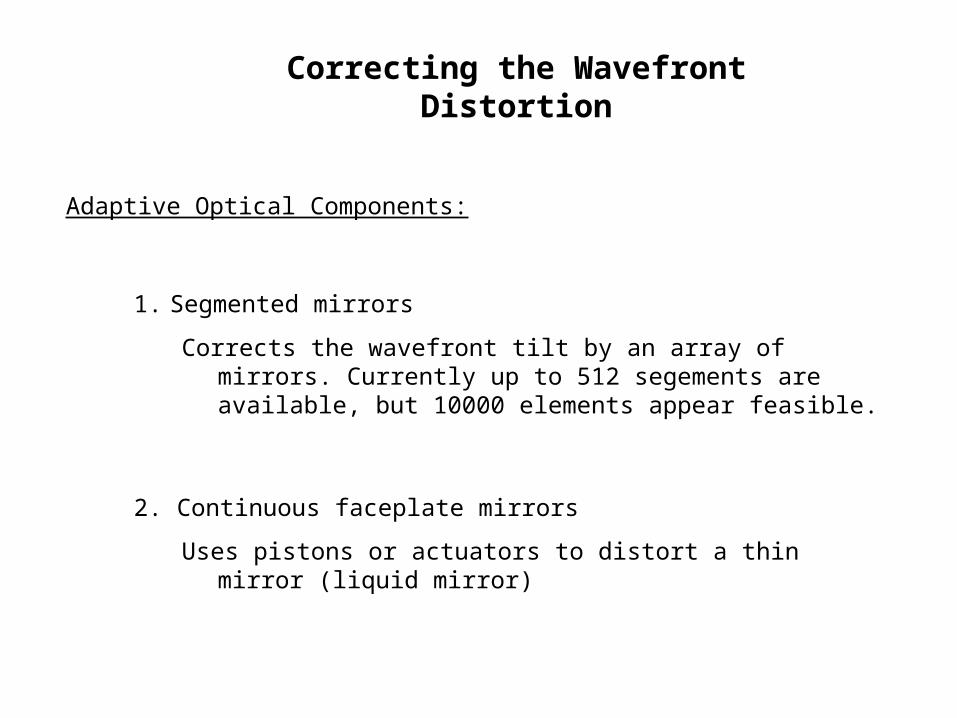
Correcting the Wavefront Distortion
Adaptive Optical Components:
1. Segmented mirrors
Corrects the wavefront tilt by an array of mirrors. Currently up to 512 segements are available, but 10000 elements appear feasible.
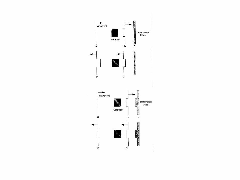
2. Continuous faceplate mirrors
Uses pistons or actuators to distort a thin mirror (liquid mirror)
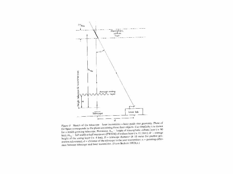
Reference Stars
You need a reference point source (star) for the wavefront measurement. The reference star must be within the isoplanatic angle, of about 10-30 arcseconds
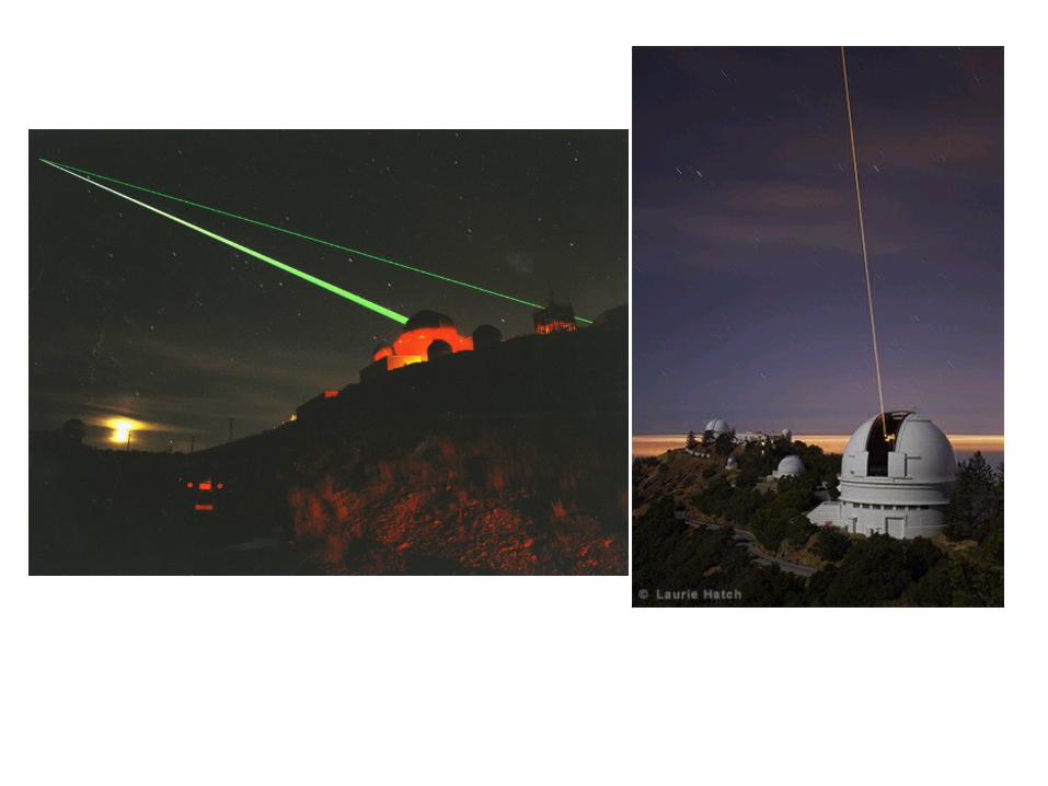
If there is no bright (mag ~ 14-15) nearby star then you must use an artificial star or „laser guide star“.
All laser guide AO systems use a sodium laser tuned to Na 5890 Å pointed to the 11.5 km thick layer of enhanced sodium at an altitude of 90 km.
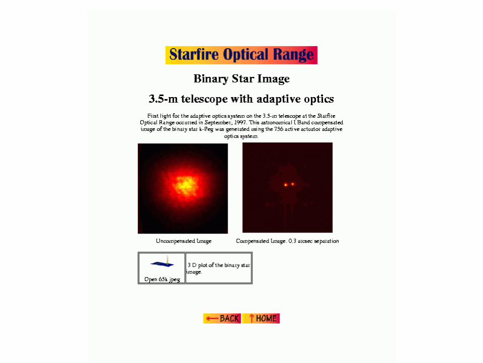
Much of this research was done by the U.S. Air Force and was declassified in the early 1990s.
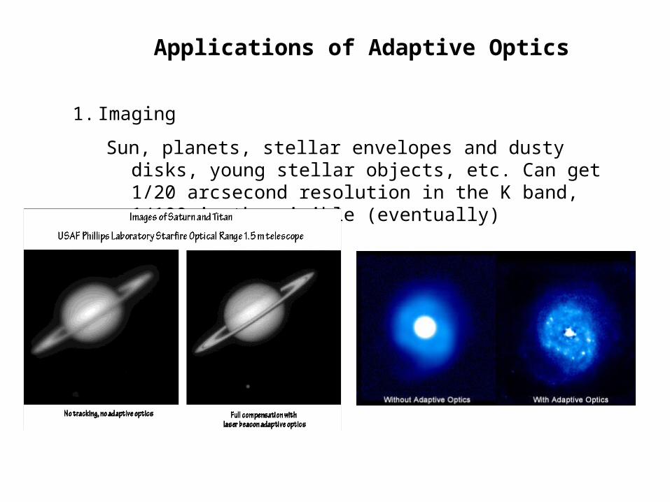
1. Imaging
Sun, planets, stellar envelopes and dusty disks, young stellar objects, etc. Can get 1/20 arcsecond resolution in the K band, 1/100 in the visible (eventually)
Applications of Adaptive Optics
Applications of Adaptive Optics
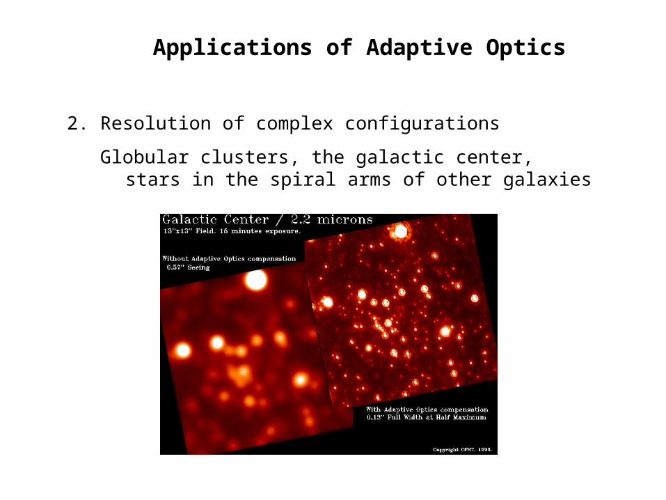
2. Resolution of complex configurations
Globular clusters, the galactic center, stars in the spiral arms of other galaxies
Applications of Adaptive Optics
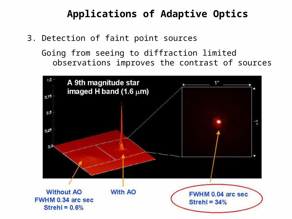
3. Detection of faint point sources
Going from seeing to diffraction limited observations improves the contrast of sources by SR D2/r0
2.
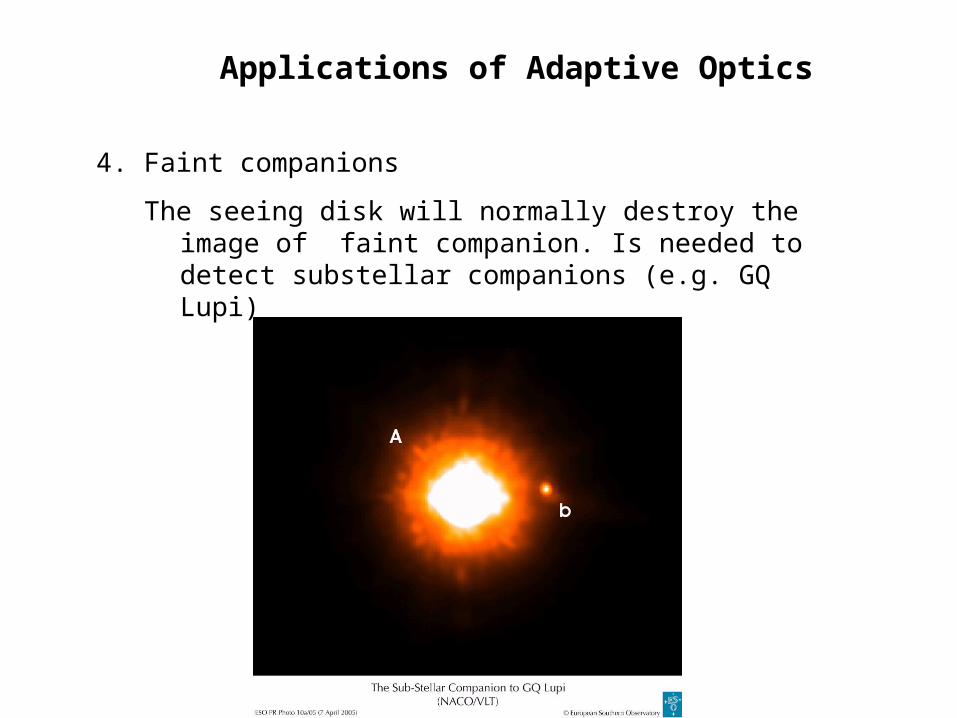
4. Faint companions
The seeing disk will normally destroy the image of faint companion. Is needed to detect substellar companions (e.g. GQ Lupi)
Applications of Adaptive Optics
Applications of Adaptive Optics
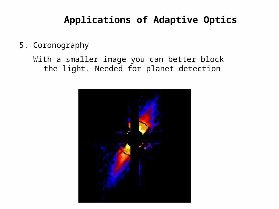
5. Coronography
With a smaller image you can better block the light. Needed for planet detection
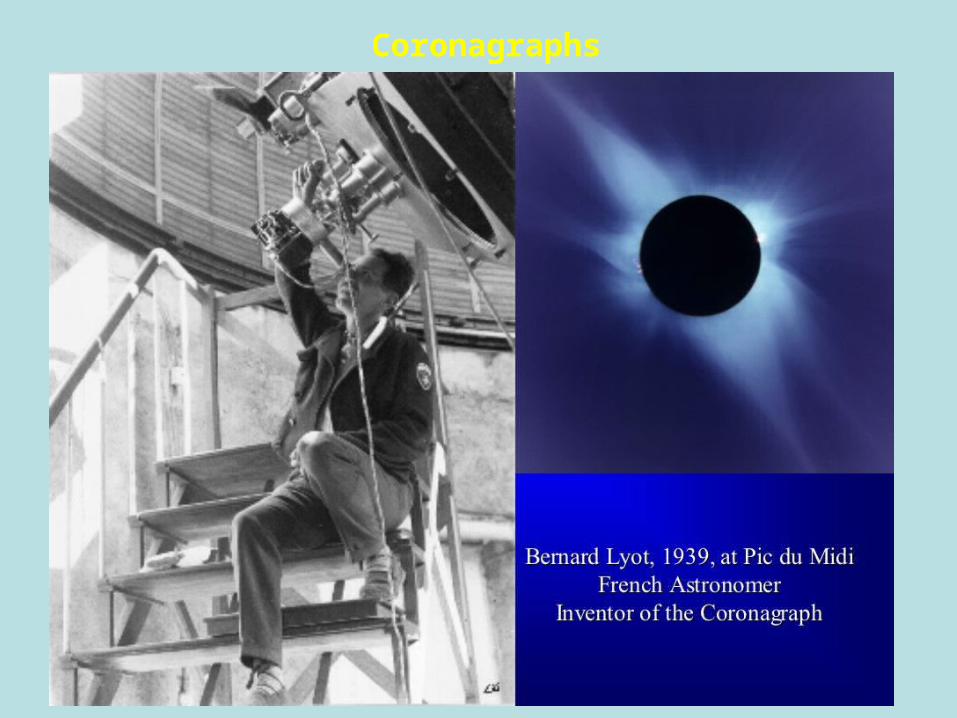
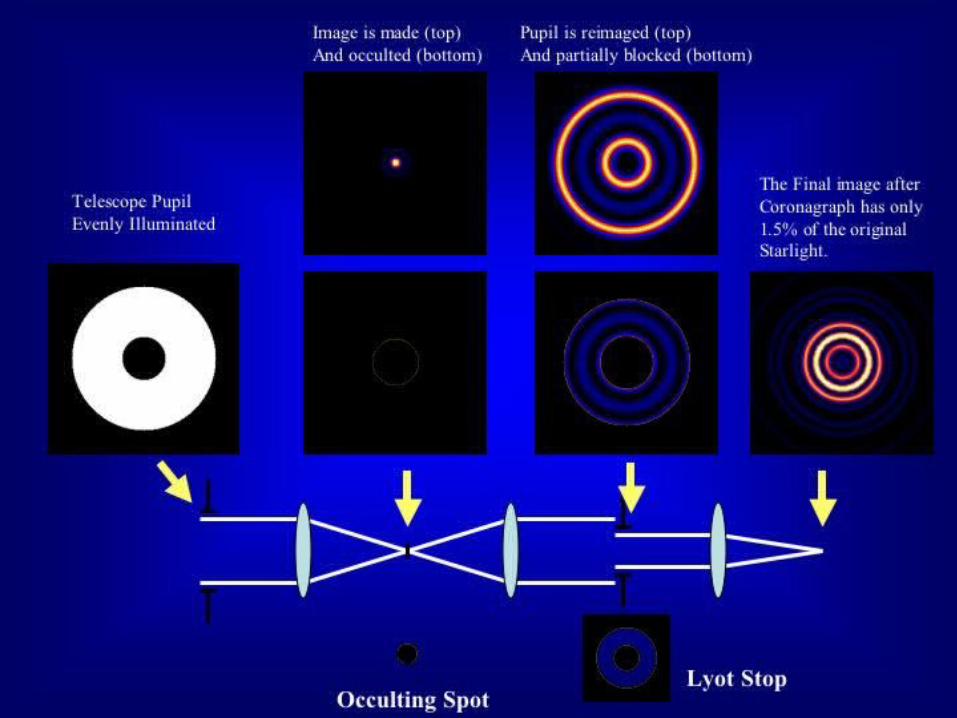
Coronagraphs
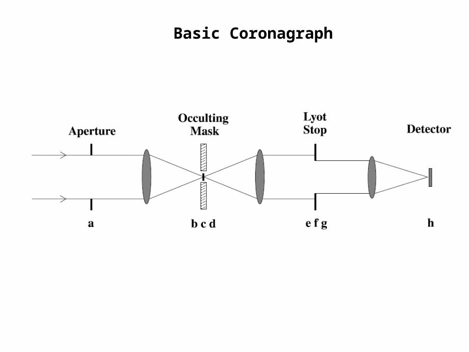
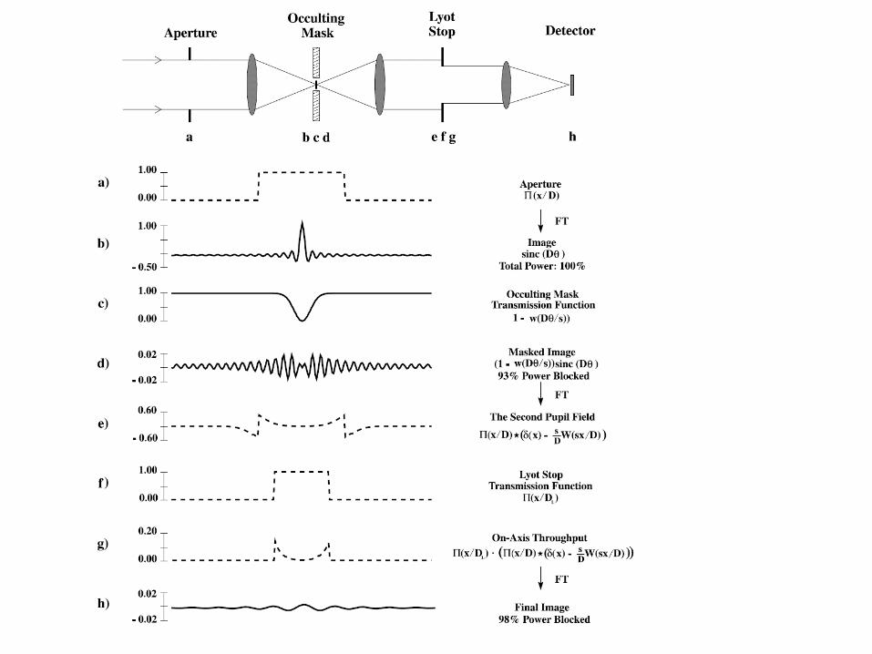
Basic Coronagraph
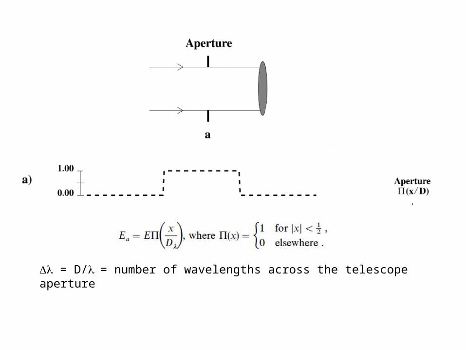
= D/= number of wavelengths across the telescope aperture
b)
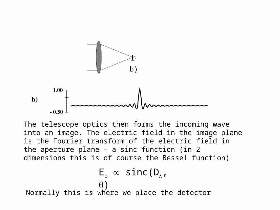
The telescope optics then forms the incoming wave into an image. The electric field in the image plane is the Fourier transform of the electric field in the aperture plane – a sinc function (in 2 dimensions this is of course the Bessel function)
Eb ∝ sinc(D, )
Normally this is where we place the detector
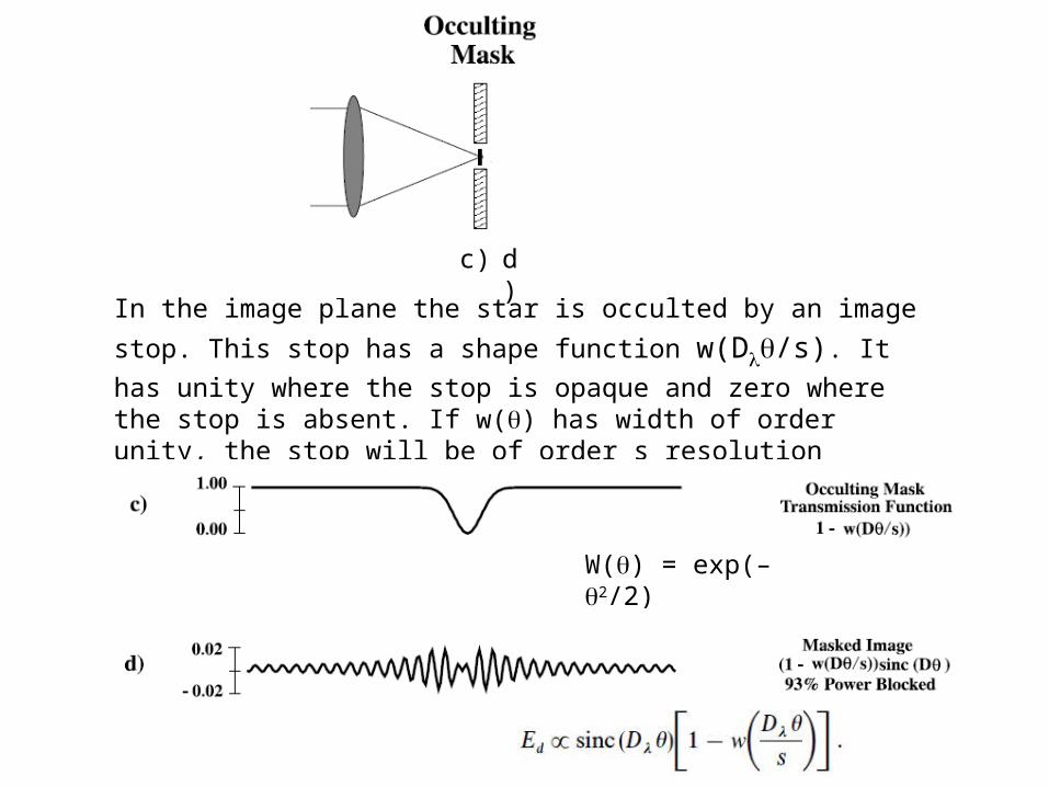
In the image plane the star is occulted by an image stop. This stop has
a shape function w(D/s). It has unity where the stop is opaque and
zero where the stop is absent. If w() has width of order unity, the stop will be of order s resolution elements. The transfer function in the
image planet is 1 – w(D/s).
c)
W() = exp(–2/2)
d)
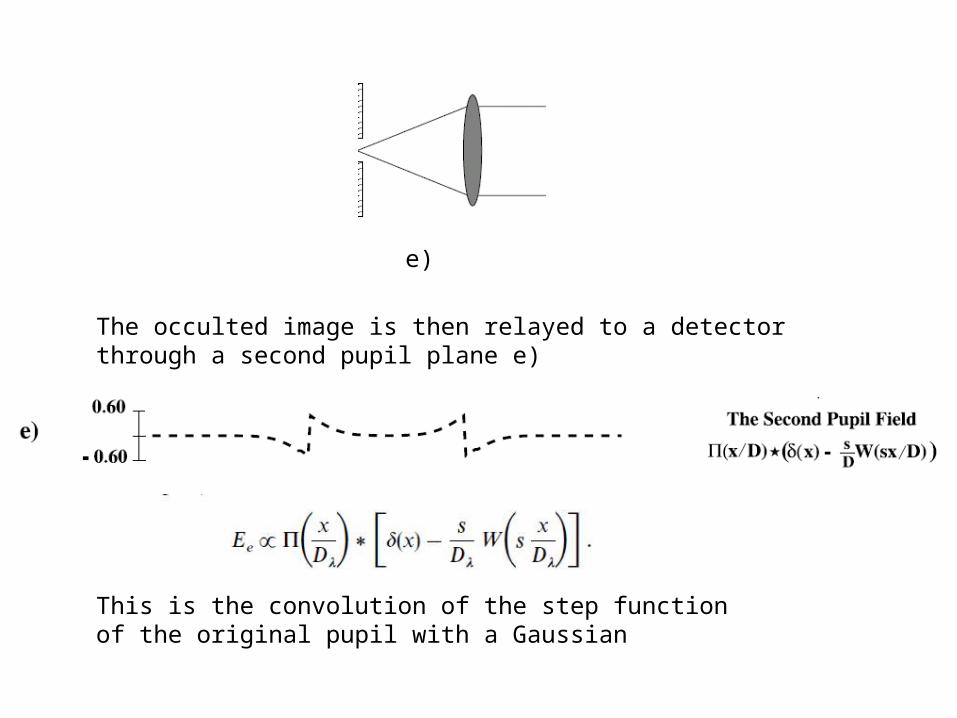
The occulted image is then relayed to a detector through a second pupil plane e)
e)
This is the convolution of the step function of the original pupil with a Gaussian
e)
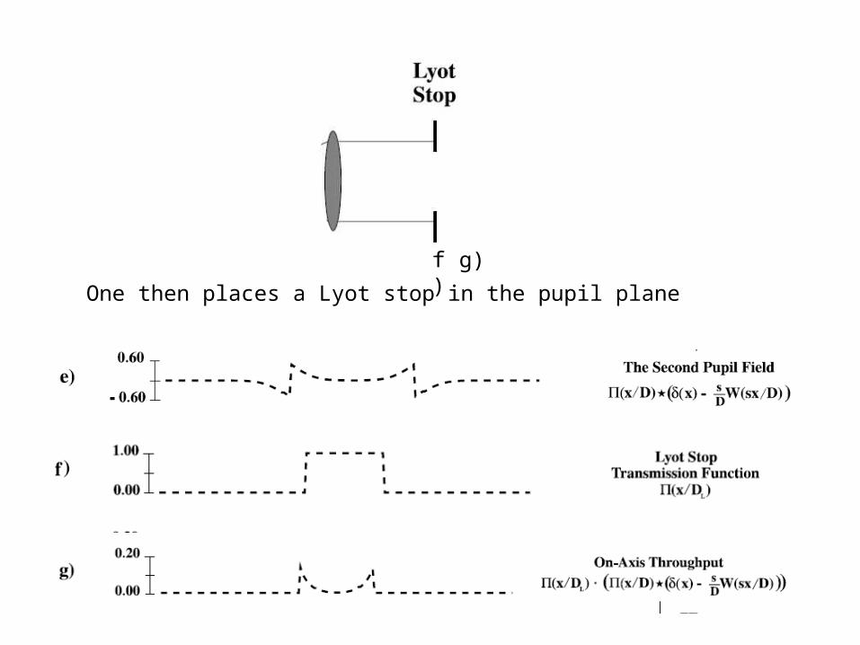
One then places a Lyot stop in the pupil plane
f) g)
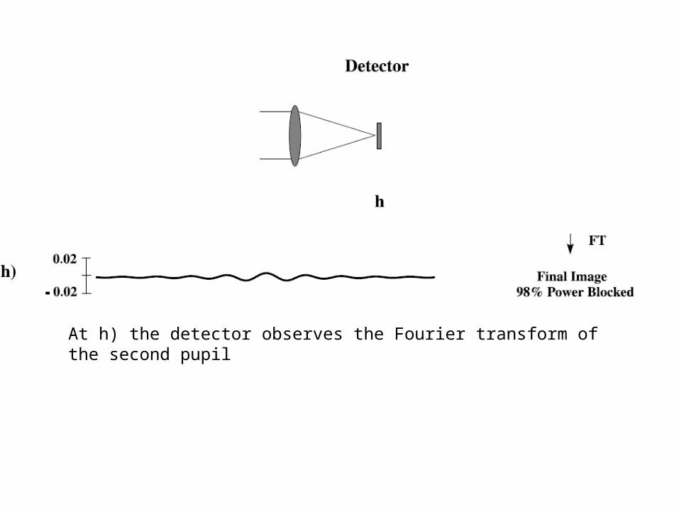
At h) the detector observes the Fourier transform of the second pupil
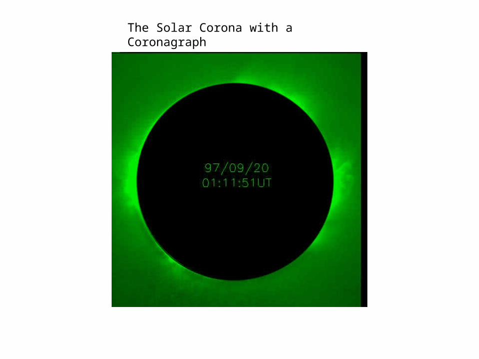
The Solar Corona with a Coronagraph
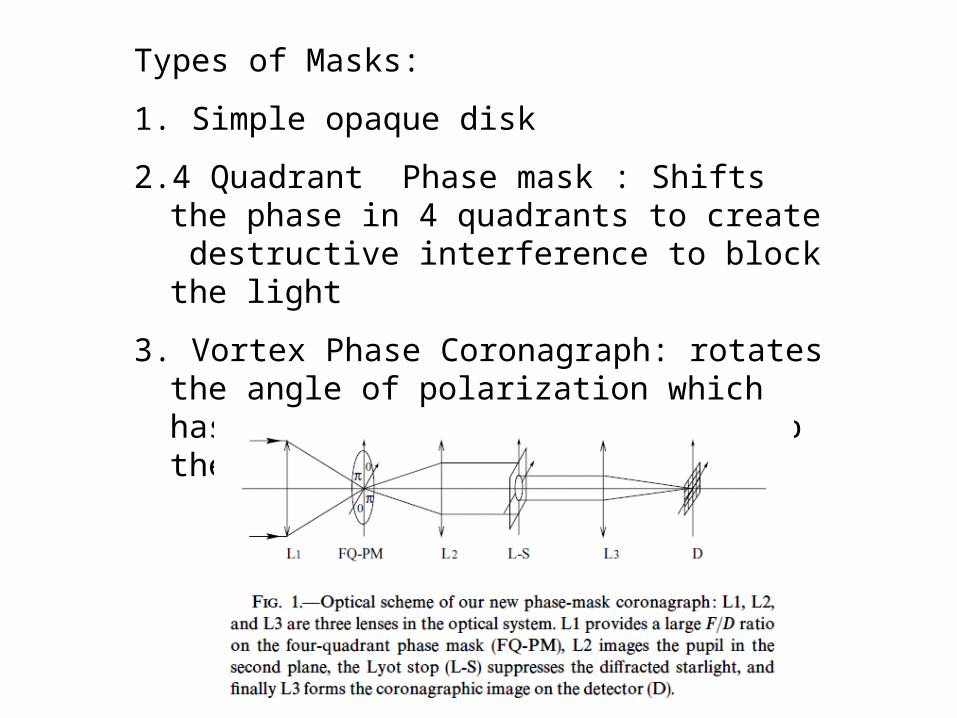
Types of Masks:
1. Simple opaque disk
2. 4 Quadrant Phase mask : Shifts the phase in 4 quadrants to create destructive interference to block the light
3. Vortex Phase Coronagraph: rotates the angle of polarization which has the same effect as ramping up the phase shift
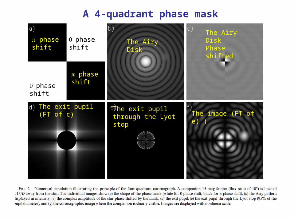
A 4-quadrant phase mask
phase shift
phase shift
phase shift
phase shift
The Airy Disk
The Airy Disk Phase shifted
The exit pupil (FT of c)
The exit pupil through the Lyot stop The image (FT of e) )
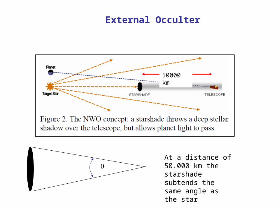
External Occulter
50000 km
At a distance of 50.000 km the starshade subtends the same angle as the star
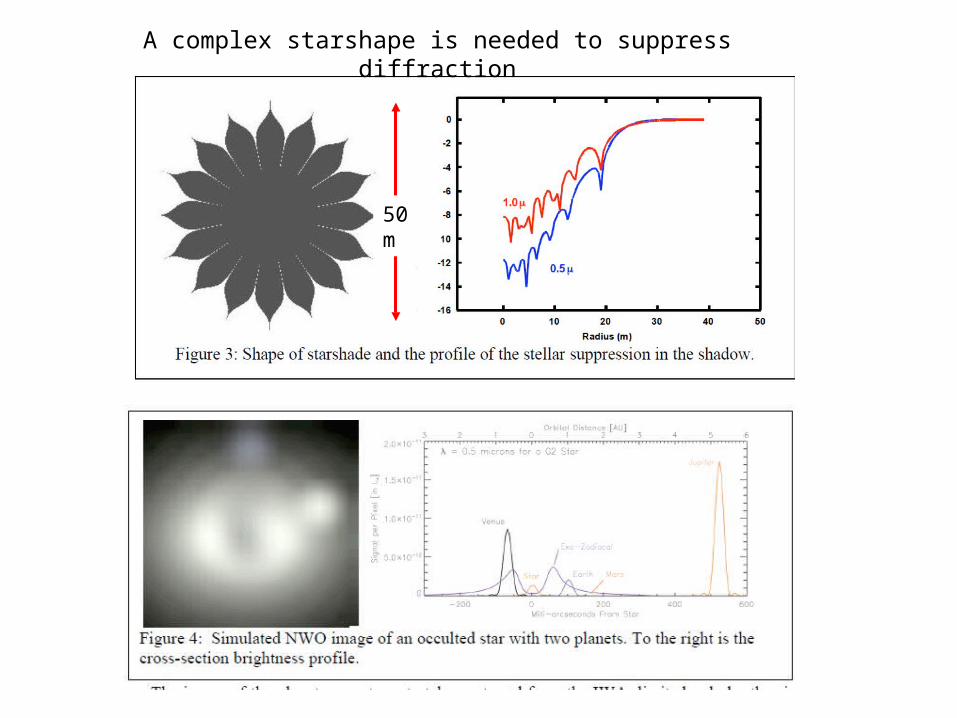
50 m
A complex starshape is needed to suppress diffraction
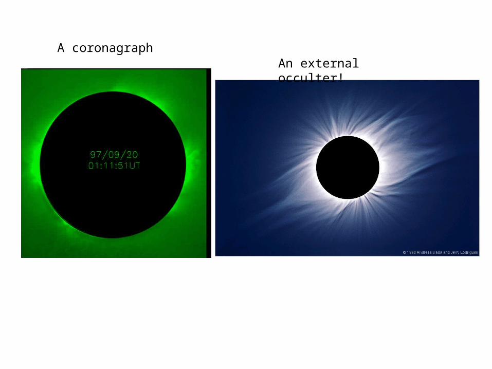
A coronagraphAn external occulter!
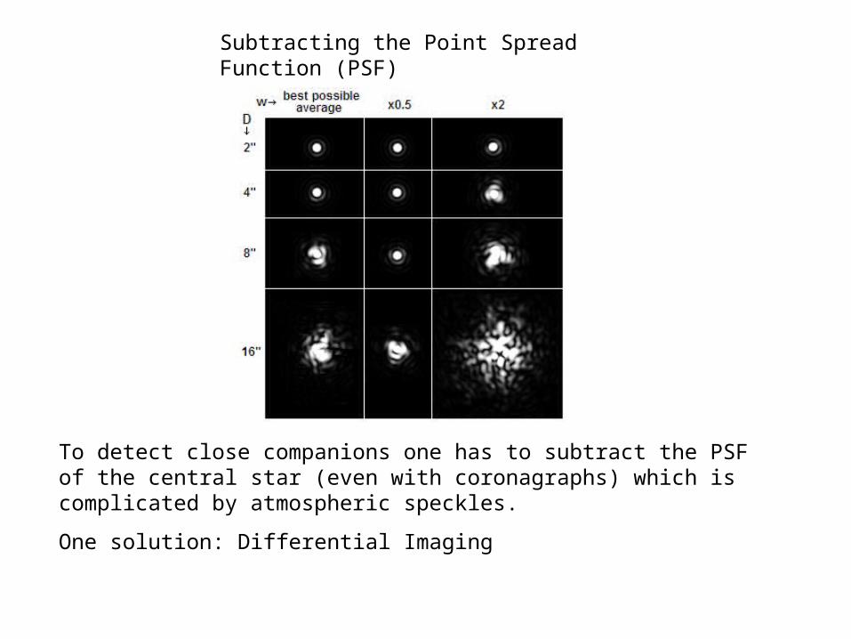
Subtracting the Point Spread Function (PSF)
To detect close companions one has to subtract the PSF of the central star (even with coronagraphs) which is complicated by atmospheric speckles.
One solution: Differential Imaging
1.58 m 1.68 m
1.625 m
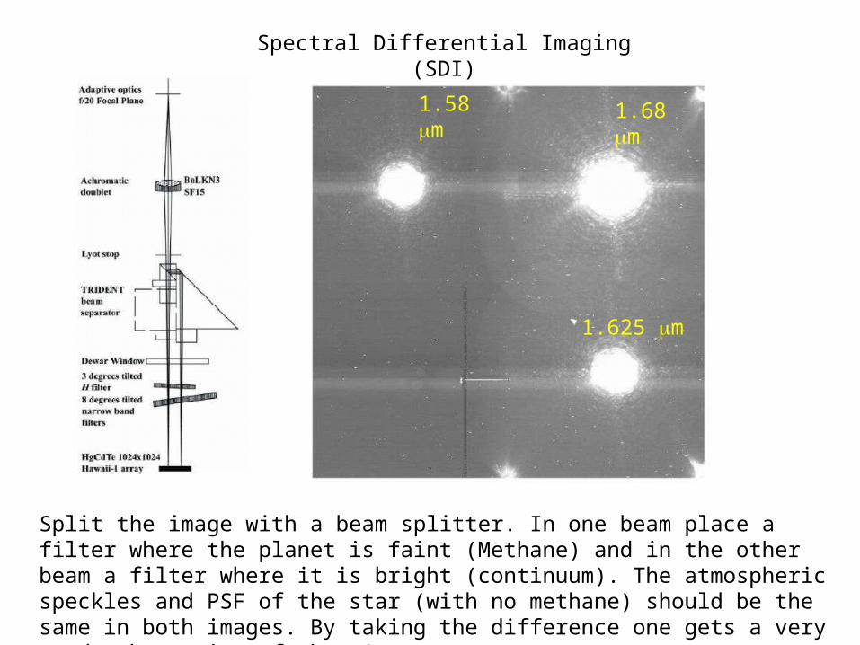
Spectral Differential Imaging (SDI)
Split the image with a beam splitter. In one beam place a filter where the planet is faint (Methane) and in the other beam a filter where it is bright (continuum). The atmospheric speckles and PSF of the star (with no methane) should be the same in both images. By taking the difference one gets a very good subtraction of the PSF
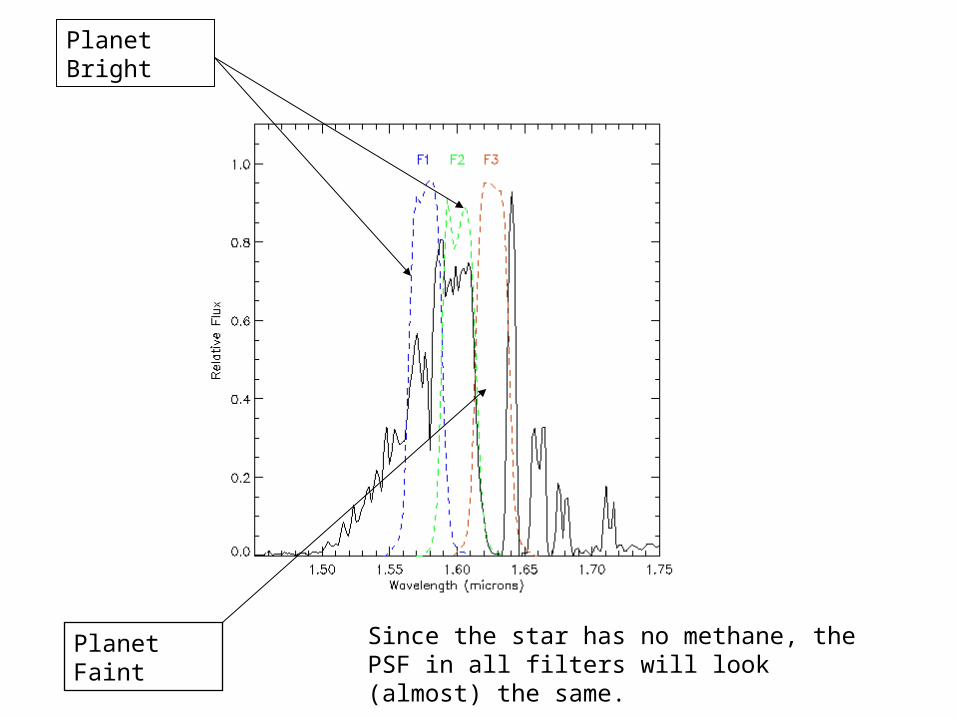
Planet Bright
Planet Faint Since the star has no methane, the PSF in all filters will look (almost) the same.
Nulling Interferometry
Principles of Long Baseline Stellar Interferometry, ed. Peter Lawson
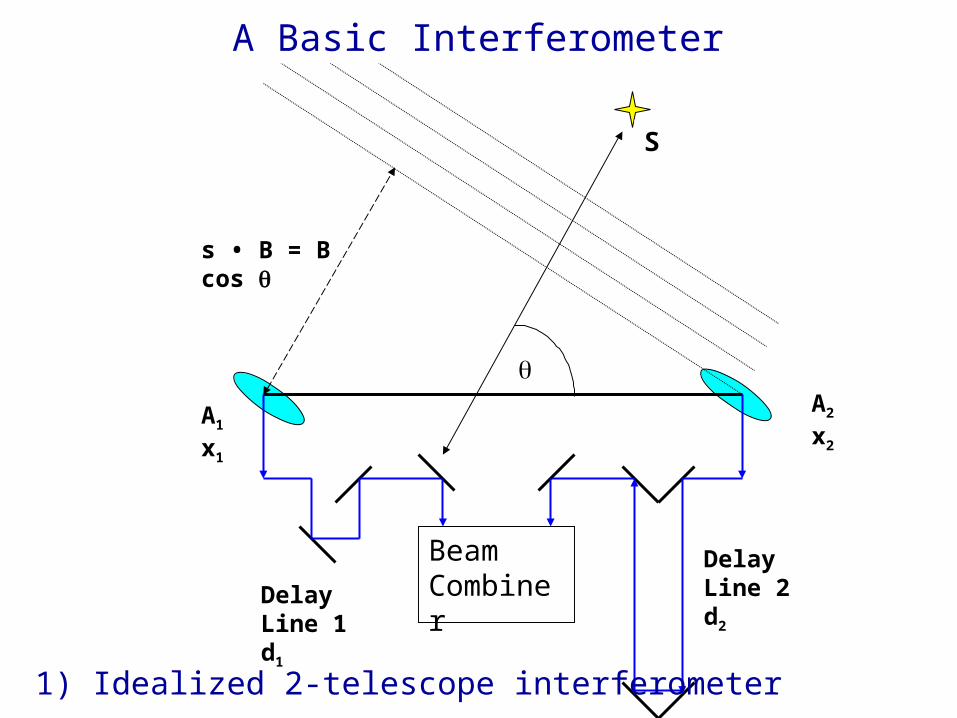
A1
x1
Beam Combiner
A2
x2
Delay Line 1d1
Delay Line 2d2
s • B = B cos
S
A Basic Interferometer
1) Idealized 2-telescope interferometer
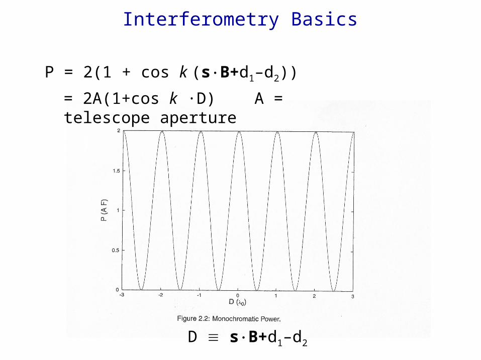
Interferometry Basics
D sB+d1–d2
P = 2(1 + cos k (sB+d1–d2))
= 2A(1+cos k ·D) A = telescope aperture
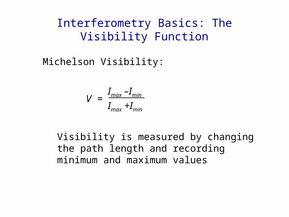
Interferometry Basics: The Visibility Function
Michelson Visibility:
V = Imax –Imin
Imax +Imin
Visibility is measured by changing the path length and recording minimum and maximum values
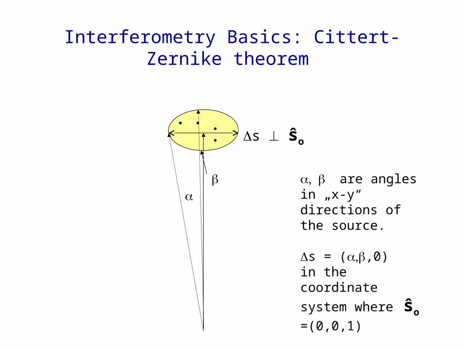
Interferometry Basics: Cittert-Zernike theorem
s ŝo
are angles in „x-
y“ directions of the source.
s = (,0)in the coordinate system
where ŝo =(0,0,1)
Interferometry Basics: Cittert-Zernike theorem
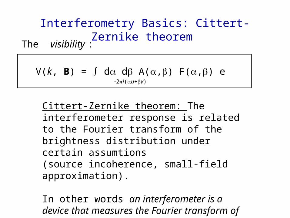
The visibility :
V(k, B) = d d A(,) F(,) e 2i(u+v)
Cittert-Zernike theorem: The interferometer response is related to the Fourier transform of the brightness distribution under certain assumtions(source incoherence, small-field approximation).
In other words an interferometer is a device that measures the Fourier transform of the brightness distribution.
Interferometry Basics: Cittert-Zernike theorem
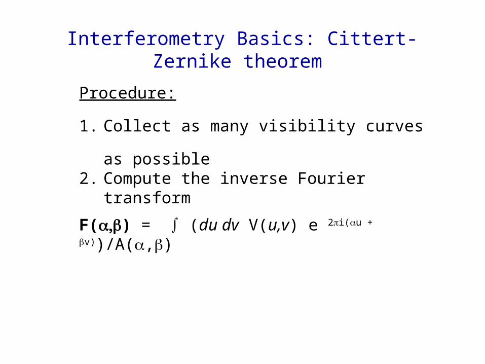
Procedure:
1. Collect as many visibility curves as possible2. Compute the inverse Fourier transform
F() = ∫ (du dv V(u,v) e 2i(u + v))/A(,)
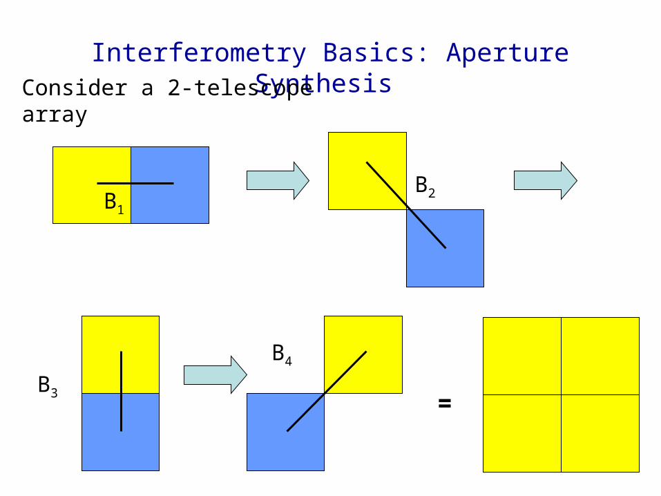
Interferometry Basics: Aperture Synthesis
Consider a 2-telescope array
=
B1
B2
B3
B4
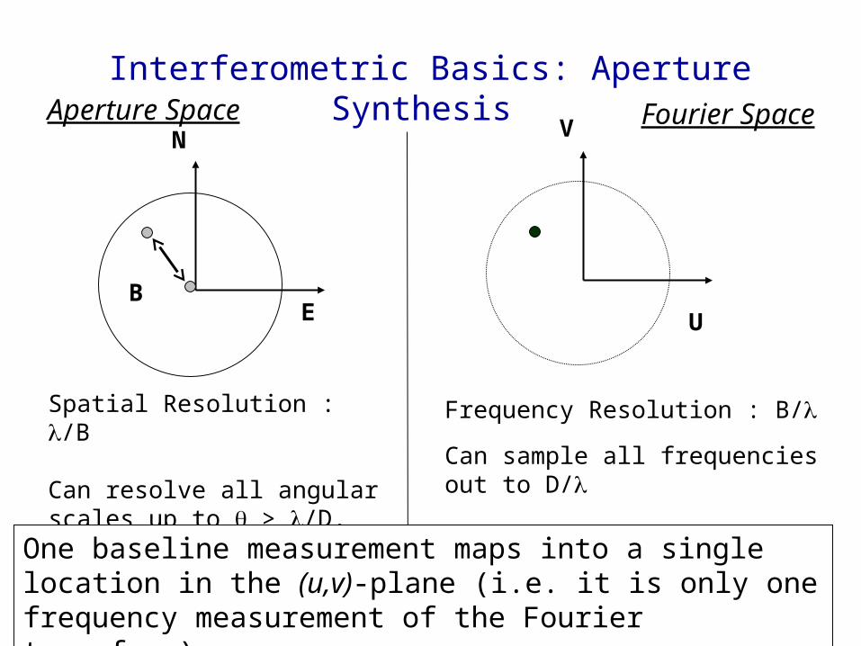
Interferometric Basics: Aperture Synthesis Aperture Space Fourier Space
N
EB
V
U
Spatial Resolution : /B Can resolve all angular scales up to > /D, i.e. the diffraction limit
Frequency Resolution : B/
Can sample all frequencies out to D/
One baseline measurement maps into a single location in the (u,v)-plane (i.e. it is only one frequency measurement of the Fourier transform)
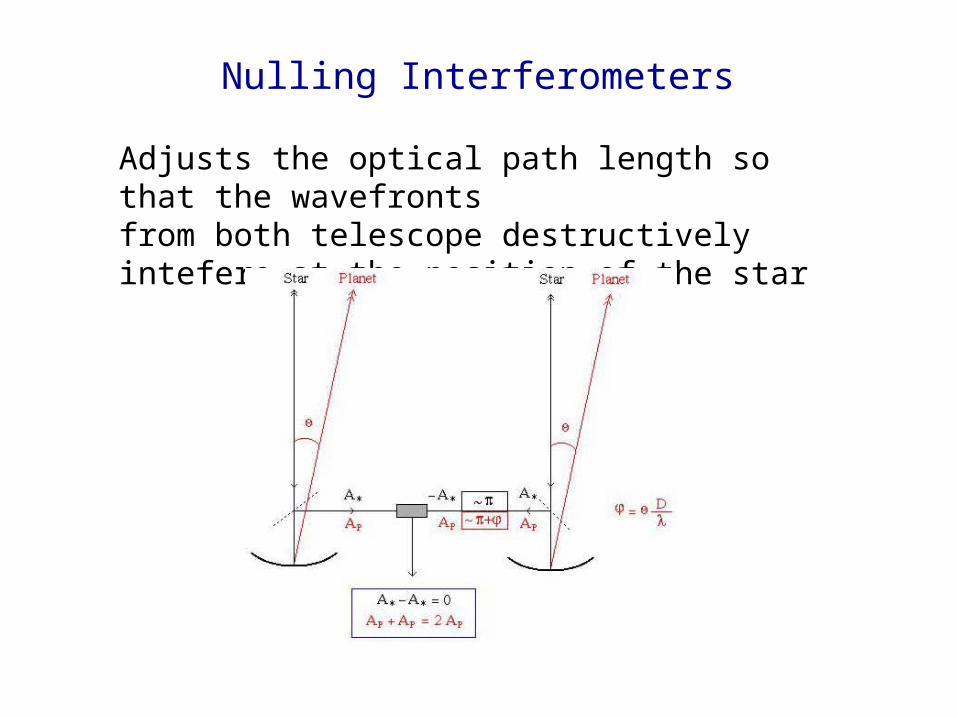
Nulling Interferometers
Adjusts the optical path length so that the wavefrontsfrom both telescope destructively intefere at the position of the star
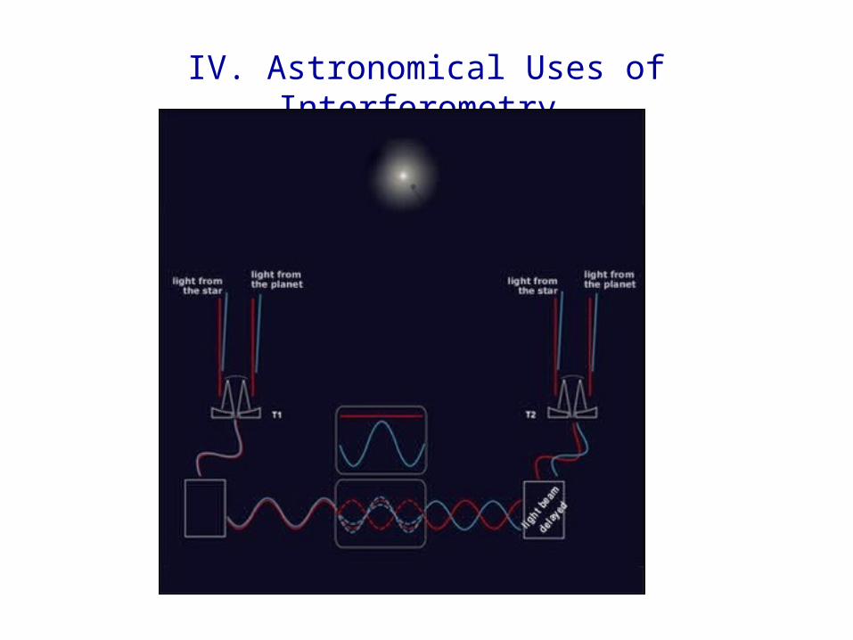
IV. Astronomical Uses of Interferometry
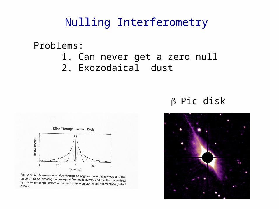
Nulling Interferometry
Problems: 1. Can never get a zero null2. Exozodaical dust
Pic disk
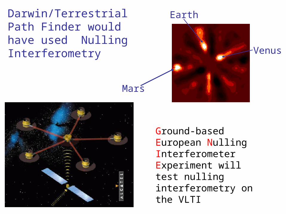
Darwin/Terrestrial Path Finder would have used Nulling Interferometry
Mars
Earth
Venus
Ground-based European Nulling Interferometer Experiment will test nulling interferometry on the VLTI

Results!
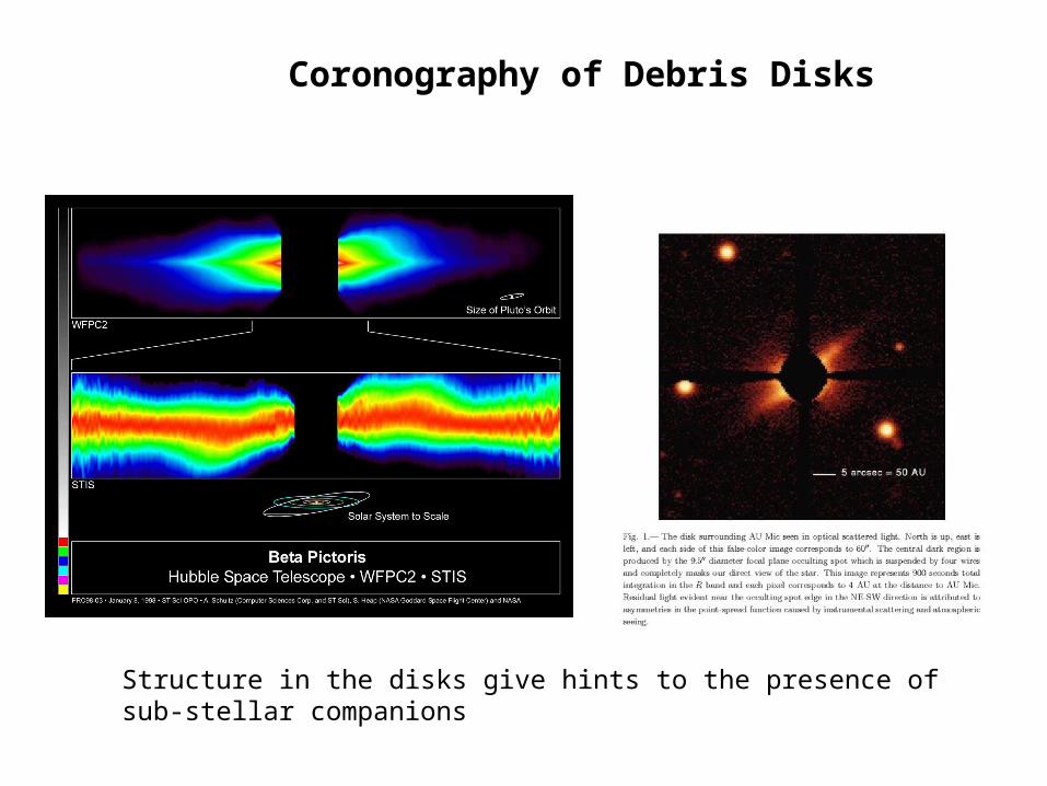
Coronography of Debris Disks
Structure in the disks give hints to the presence of sub-stellar companions
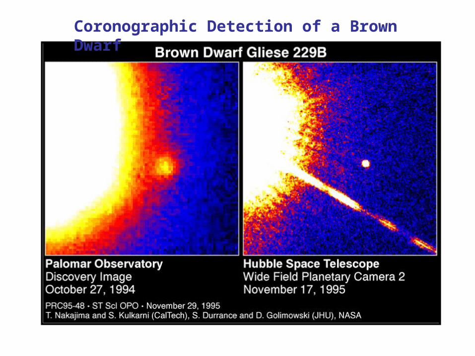
Coronographic Detection of a Brown Dwarf
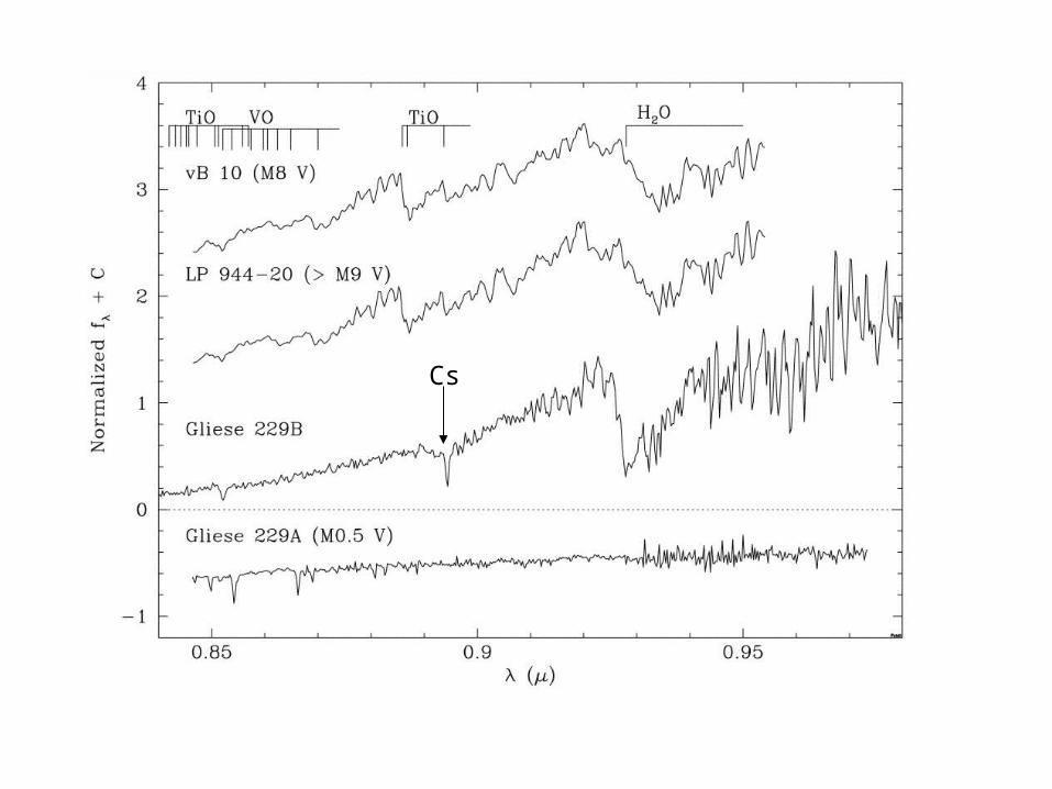
Cs
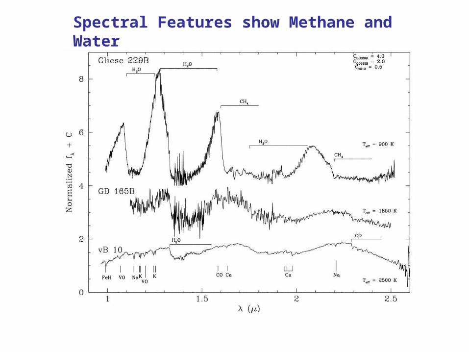
Spectral Features show Methane and Water
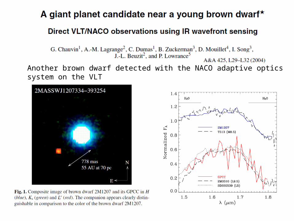
Another brown dwarf detected with the NACO adaptive optics system on the VLT
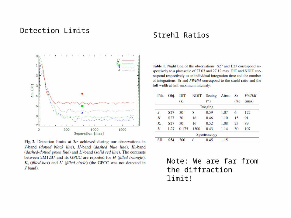
Detection LimitsStrehl Ratios
Note: We are far from the diffraction limit!
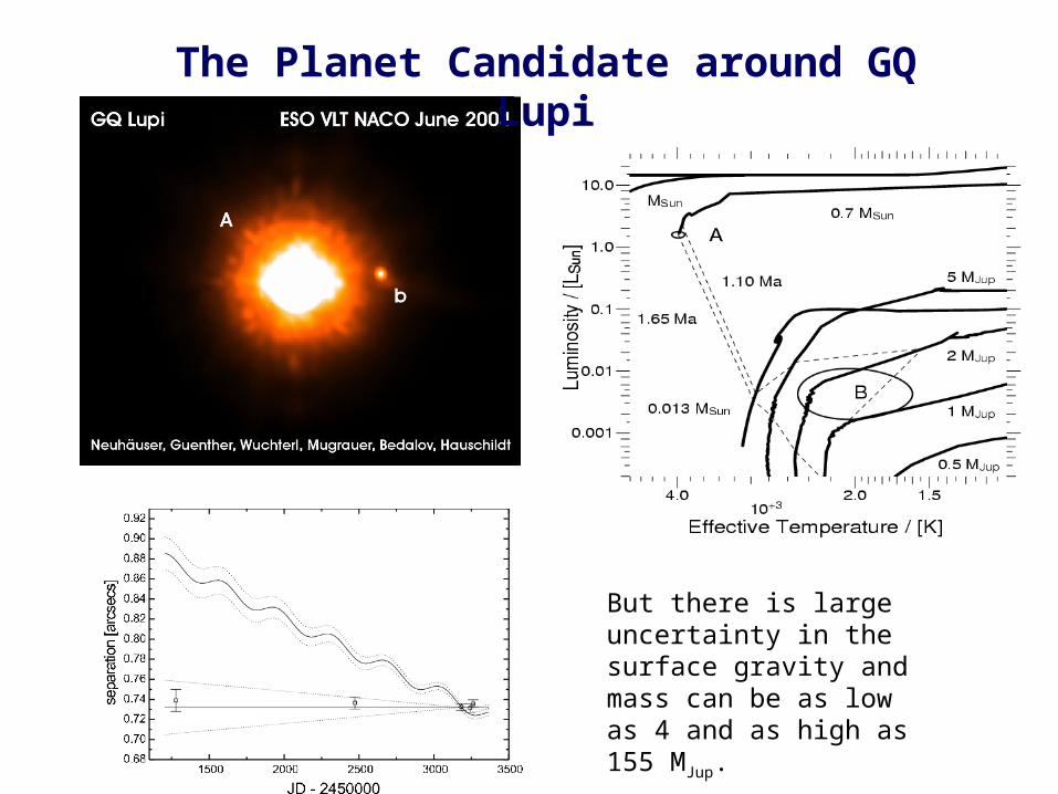
But there is large uncertainty in the surface gravity and mass can be as low as 4 and as high as 155 MJup.
The Planet Candidate around GQ Lupi
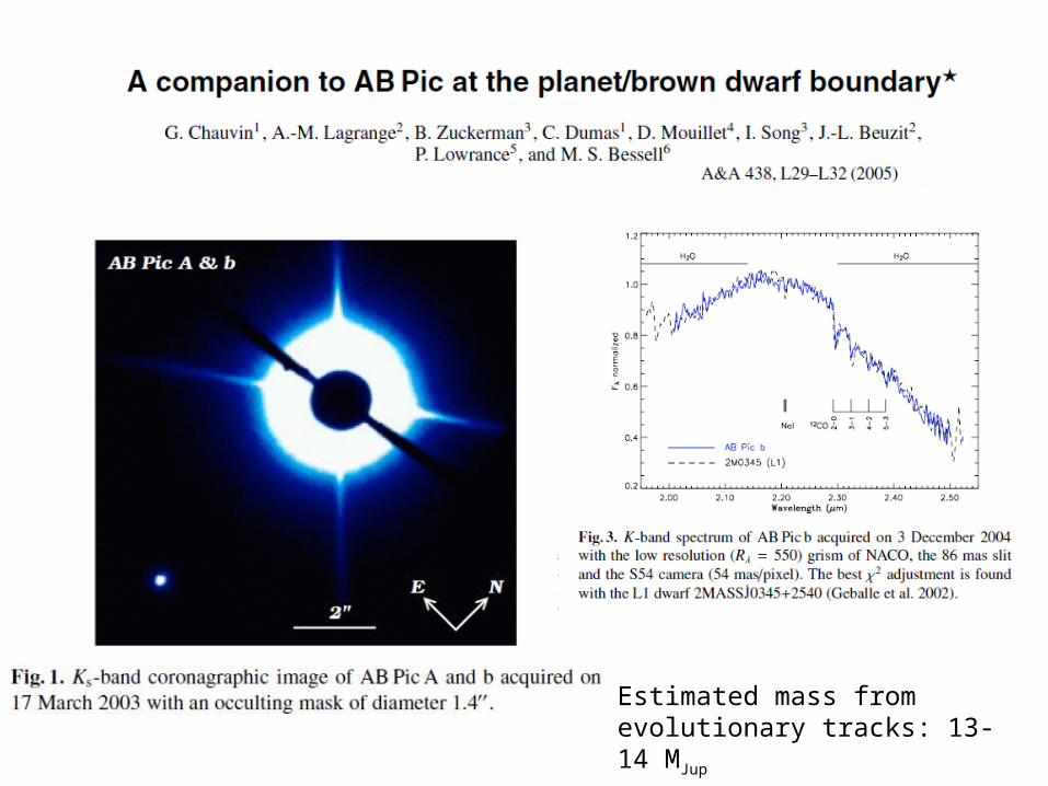
Estimated mass from evolutionary tracks: 13-14 MJup
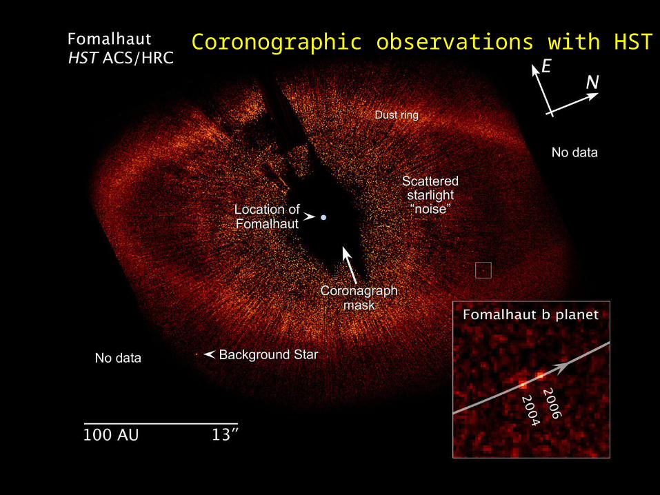
Coronographic observations with HST
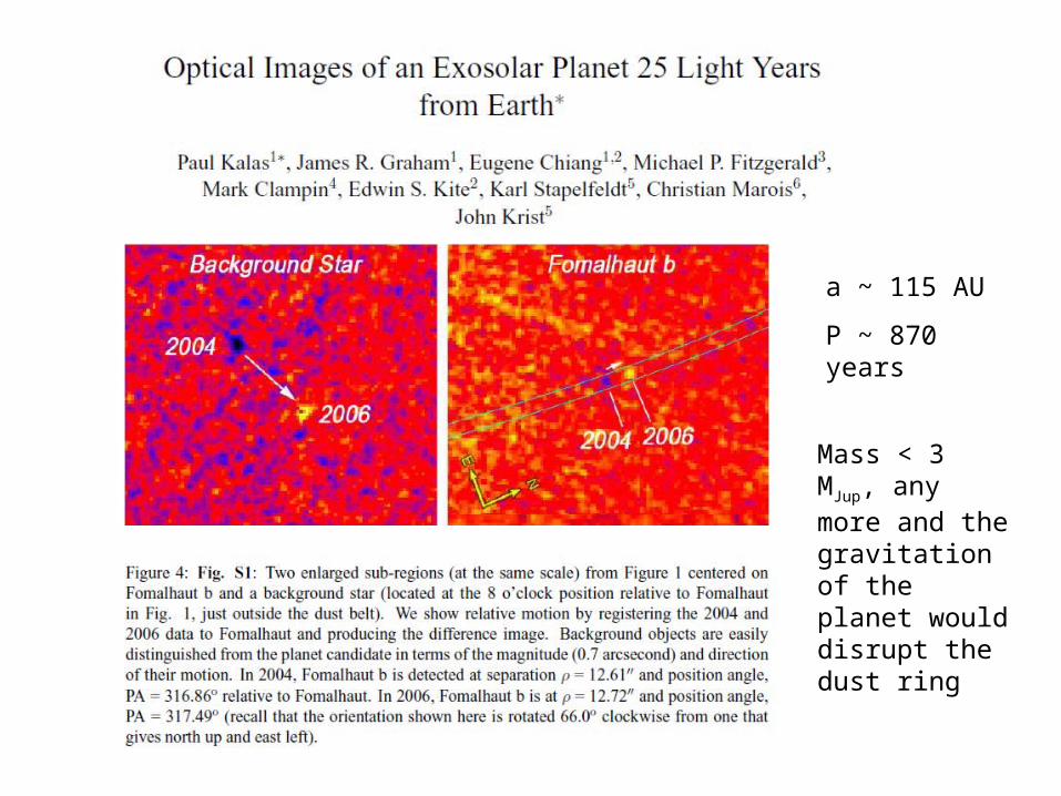
a ~ 115 AU
P ~ 870 years
Mass < 3 MJup, any more and the gravitation of the planet would disrupt the dust ring
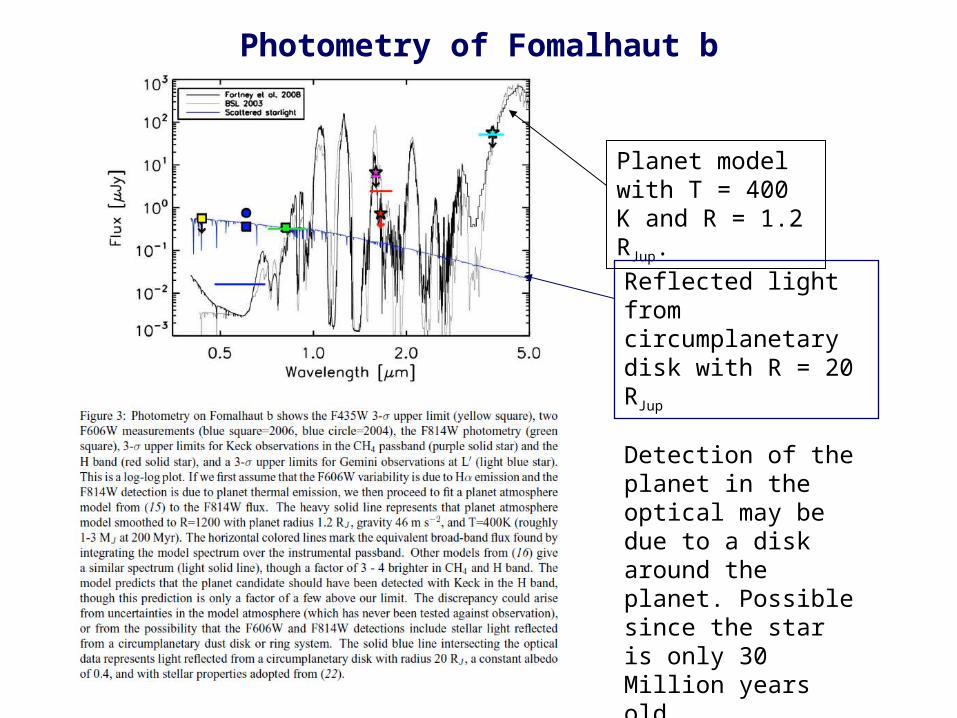
Photometry of Fomalhaut b
Planet model with T = 400 K and R = 1.2 RJup.
Reflected light from circumplanetary disk with R = 20 RJup
Detection of the planet in the optical may be due to a disk around the planet. Possible since the star is only 30 Million years old.
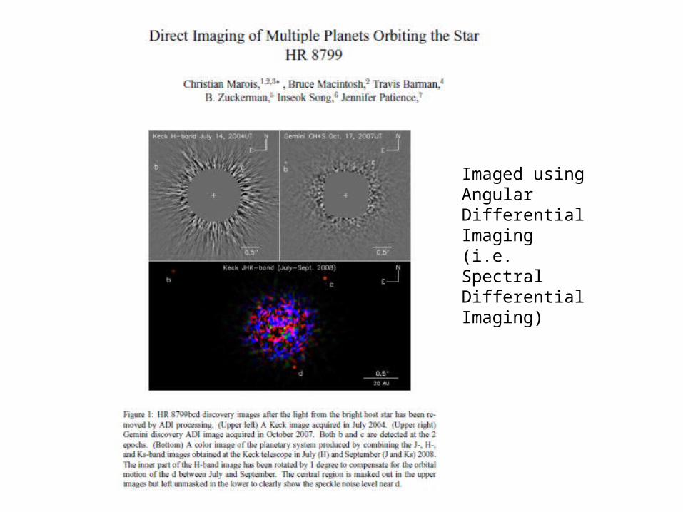
Imaged using Angular Differential Imaging (i.e. Spectral Differential Imaging)
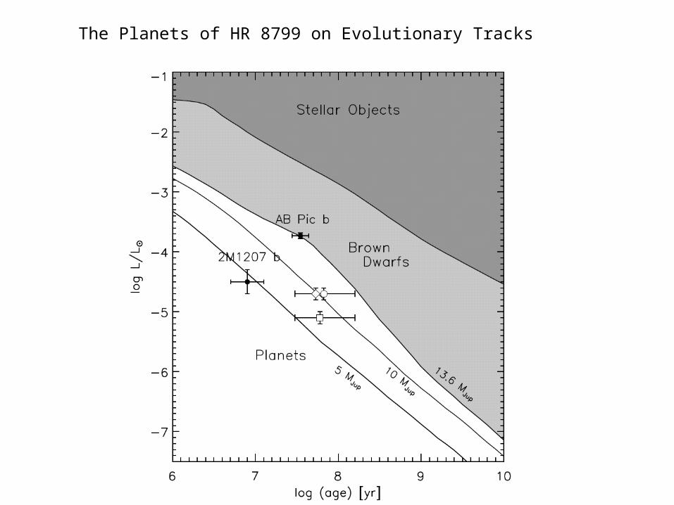
The Planets of HR 8799 on Evolutionary Tracks
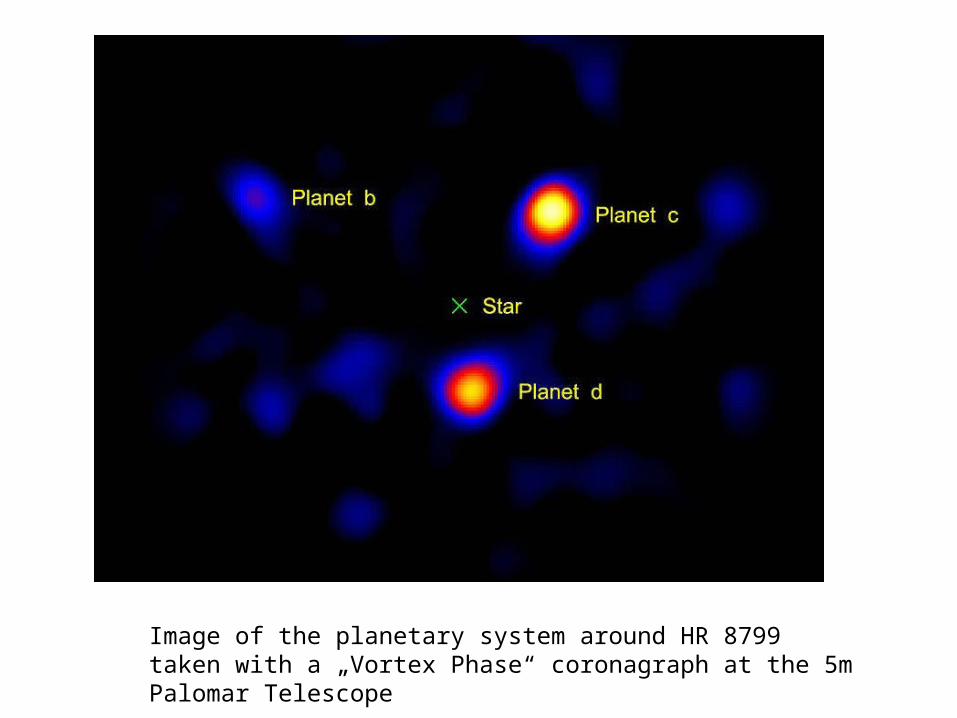
Image of the planetary system around HR 8799 taken with a „Vortex Phase“ coronagraph at the 5m Palomar Telescope
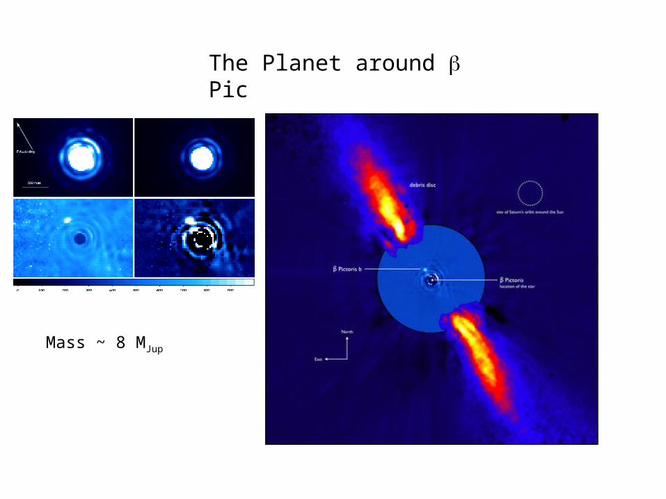
The Planet around Pic
Mass ~ 8 MJup
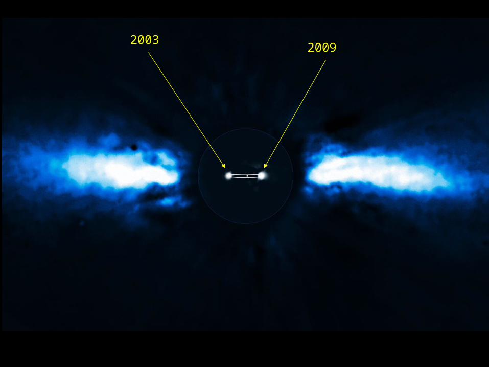
20032009
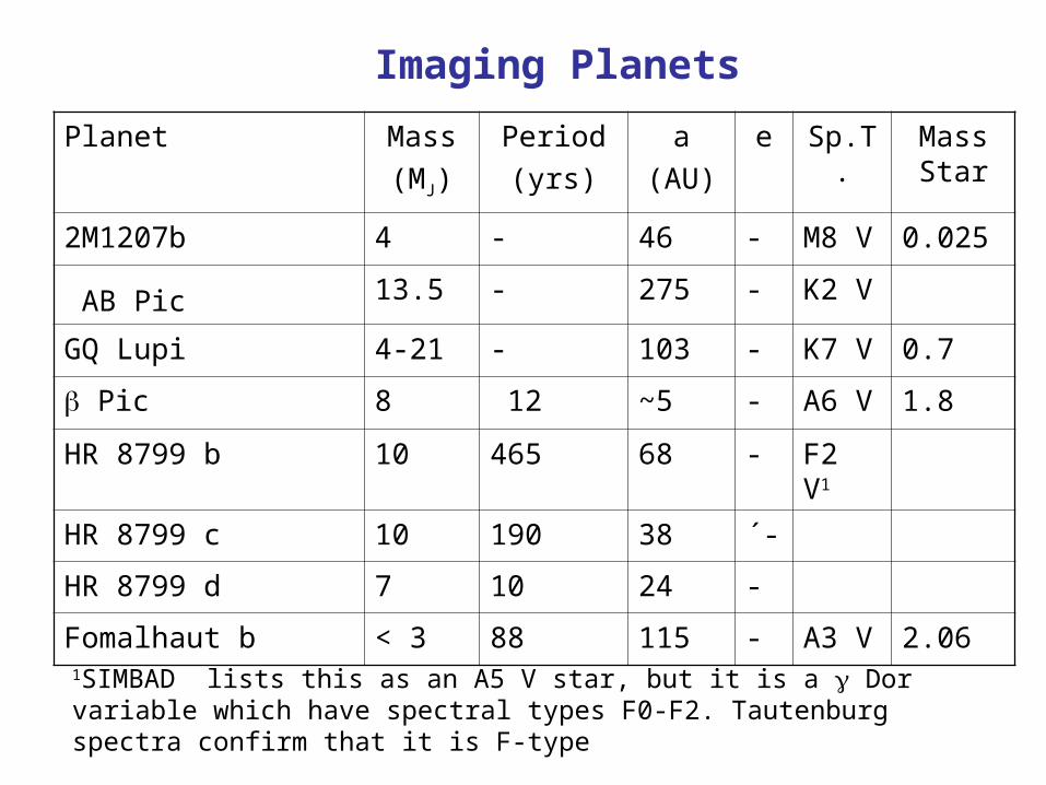
Planet Mass
(MJ)
Period
(yrs)
a
(AU)
e Sp.T. Mass Star
2M1207b 4 - 46 - M8 V 0.025
AB Pic 13.5 - 275 - K2 V
GQ Lupi 4-21 - 103 - K7 V 0.7
Pic 8 12 ~5 - A6 V 1.8
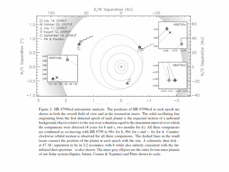
HR 8799 b 10 465 68 - F2 V1
HR 8799 c 10 190 38 ´-
HR 8799 d 7 10 24 -
Fomalhaut b < 3 88 115 - A3 V 2.06
Imaging Planets
1SIMBAD lists this as an A5 V star, but it is a Dor variable which have spectral types F0-F2. Tautenburg spectra confirm that it is F-type


![1111111111111111111inuun1111111111u - NASA · Nulling Coronagraph," SPIE Tech Inst for Detect of Exoplan-ets, pp. 217-228, 2003.]. Fiberguide developed 2D fiber arrays comprising](https://img.pdfslide.us/doc/110x75/5f0f9e197e708231d4450de4/1111111111111111111inuun1111111111u-nasa-nulling-coronagraph-spie-tech.jpg)