Direct Generation of Contour Files from Constructive Solid GeometryRepresentations

Sashidhar Guduri, Research AssistantRichard H. Crawford, Assistant Professor

Joseph J. Beaman, ProfessorDepartment of Mechanical Engineering

The University of Texas at AustinAustin, TX 78712

Abstract

Geometry processing for layer-based Solid Freeform Fabrication consists of at least twosteps: slicing the geometry to obtain the part contours for each layer, and scan-converting thelayers for laser scanning (or other device-dependent in-layer processing). This paper discussesthe generation of contour files directly from Constructive Solid Geometry (CSG) representationsfor the Selective Laser Sintering process. Previous work at The University of Texas focused onslicing CSG representations composed of quadric primitives. This paper extends previous workat UT to include the torus, a fourth degree surface, as one of the CSG primitives. Slicing a torusresults in a fourth degree equation in two variables, which represents a curve in two-dimensionalreal space. For. some special cases, this fourth degree equation may be sub-divided into twosecond degree equations. For the cases where the fourth degree equation cannot be sub-divided,a method is presented to approximate the fourth degree curve with second degree curvesegments.

Introduction

Solid Freeform Fabrication (SFF) techniques manufacture solid objects directly fromthree-dimensional computer models. Most SFF processes produce parts on a layer-by-Iayerbasis. process begins by slicing the geometric description of the part into layers. The slicingoperation generates the contours of the part for each layer. The contours are then processed in amanner dependent upon the particular SFF technology. For instance, for Selective LaserSintering (SLS) the contours are discretized into "toggle points" at which the laser beam must bemodulated to produce the desired solid.

geometric description used to represent solid objects significantly affects theaccuracy and quality of the final parts produce with SFF. One way to improve the final accuracyand definition of SFF parts is to improve the. geometric descriptions that represent threedimensional objects. As described in [1], ConstructiveSQlidGeometry is one geometricdescription where the accuracy iofthe final contours can be improved as compared to presentgeometric representations. A method was presented in [1] for generating contour files fromConstructive Solid Geometry representations composed of quadric objects. This paper extendsthat work to include higher degree surfaces (degree greater than two) in the primitive set.Special attention is given to the torus, a fourth degree surface.

Slicing a higher degree surface results in a boundary curve whose degree may be greaterthan two. A curvec)f degree .greater than two is parametrizable if the genus (g) of the curve iszero. The genus of a curve is defined by

291

g = (N -l)~N - 2) _ ~O(p),I

(1)

where N is the degree oftheeq1Jation and the O(Pi) operator appropriately countsthe number oftimes that the curve comes in contact with itstelf at each singular point Pi' All quadratic curvesare genus zero and are therefore parametri~able. A limited set of curves of degree greater thantwo are parametrizable. Unfortunately, the algebraic equations produced by many geometricdesign applications are not generally genus zero. It therefore becomes necessary to approximatehigher degree curves with lower degree curve segments. These curve segments are thenparametrized individually.

The method presented in this paper approximates curves of degree greater than two usingsecond degree curve segments. There are two advantages to using second degree curves. First,all second degree curve segments are parametrizable. Second, the intersection of two seconddegree curves (required for Boolean set operations) can be computed by well-known, stablealgorithms. If curve segments of degree greater than two are used as approximations, calculatingthe intersection of two curves becomes computationally expensive. The algorithm for generatingthe approximation is based on degree reduction of the triangular Bernstein form of the curve.The next section of the paper illustrates the representation of the torus as a CSG primitive andgives the equations involved in calculation of the implicit equation of the torus. Following thissection, a method for determining the Bernstein coefficients of the implicit curve is described.The remainder of the paper describes the steps in the approximation algorithm: parametrization,approximation and error estimation, subdivision, and resolution of singularities. Examples arepresented at the end of the paper.

Torus as a CSG Primitive

The equation of a torus generated by sweeping a circle about the y axis, with the origin atthe center, is given by:

(2)

As a CSG primitive the torus is represented using a base point, an axis vector and two radii, asillustrated in Figure 1.

Given the above information, the equation of the torus can be generated by translating thebase point of the torus to the origin and rotating about x and z axes such that the resulting axis ofthe torus is aligned with the y axis. This procedure is summarized below:

1. Normalize the axis vector of the torus.2. Translate the base of the torus to the origin.

3. Rotate about the x axis by an angle of -tan-1 (;:) •

4. Rotate about the z axis by an angle of tan-1 (..J x. J.z; +y;If the above steps are applied the following transformations are obtained

292

x

Figure 1. Representation of a torus.

z =--=====1 )

(3)

where and Z define the coordinate system local to torus. Substituting equationsinto equation 2 gives the fourth degree equation of the torus x, y and z. Substituting zvalue of the slicing plane gives a fourth degree equation in y that is the equation ofthe contour for that slicing plane.

'n.llI'1I'llTQlI'01I::'1I11'1II"lI of Algebraic EQualUOllS to

section describes a method for """.... ,,,""'...t-....,,...

triangular regions.n""",...."""" elevation of u..l.f'O.""..,.l.u..I."" ,.".,,........... ..,

of the curve. method to doa bivariate polynomial of degree N is given by:

293

(0,0, 1)

x

(1, 0)

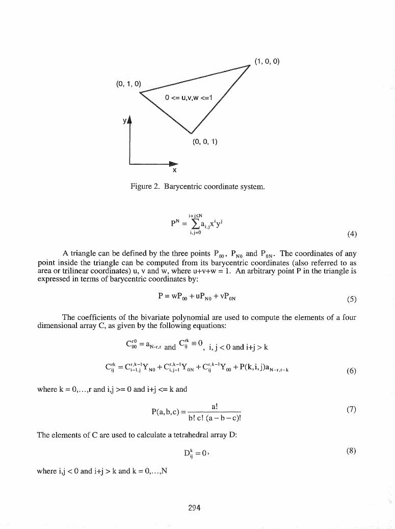
(4)

A triangle can be defined by points P00' P NO PON' The coordinates anypoint inside the triangle can be computed from its barycentric coordinates (also referred to asarea or trilinear coordinates) u, v and w, where u+v+w = 1. arbitrary point P isexpressed in terms of barycentric coordinates by:

P wPoo +

coefficients of the ...... ,,'o"".of"o

dimensional array as given by

+vPON

a

(5)

crO00 C r"k 0 .. 0

1J , 1, J < k

where k O, ... ,r

Cr k-Iy Cr k-Iy Cr k-Iy= "l' NO + '" 1 ON +.: 00 +1- ,J 1,]- 1J

>= 0 and <= k

(6)

pea, b,c) (7)

C are used to vU.lvY.J.u.""" a TaT11"0 """""111""

(8)

where i,j < 0 >k k=

Dk Dk-I X Dk- I X Dk-1X Ckkij = i-I,j NO + i,j-I ON + ij 00 + ij

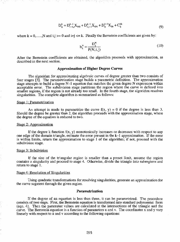
where k = O,...... ,N and i,j >=°and i+j <= k. Finally the Bernstein coefficients are given by:

N D~b.. = I)

I) P(N,i,j)

(9)

(10)

After the Bernstein coefficients are obtained, the algorithm proceeds with approximation, asdescribed in the next section.

Approximation of Higher Degree Curves

The algorithm for approximating algebraic curves of degree greater than two consists offour stages [3]. The parametrization stage builds a parametric definition. The approximationstage attempts to build a degree N-l equation that matches the given degree N expression withinacceptable error. The subdivision stage partitions the region where the curve is defined intosmaller regions, if the region is not already too small. In the fourth stage, the algorithm resolvessingularities. The complete algorithm is summarized as follows:

Stage 1: Parametrization

An attempt is made to parametrize the curve f(x, y) = °if the degree is less than 3.Should the degree be greater than 2, the algorithm proceeds with the approximation stage, wherethe degree of the equation is reduced to two.

Stage 2: Approximation

If the degree k function f(x, y) monotonically increases or decreases with respect to anyone edge of the domain triangle, estimate the error present in the k-l approximation. If the erroris within limits, return the approximation to stage 1 of the algorithm; if not, proceed with thesubdivision stage.

Stage 3: Subdivision

If the size of the triangular region is smaller than a preset limit, assume the regioncontains a singularity and proceed to stage 4. Otherwise, divide the triangle into subregions andreturn to stage 1.

Stage 4: Resolution of Singularities

Using quadratic transformations for resolving singularities, generate an approximation forthe curve segment through the given region.

Parametrization

If the de~ree of an equation is less than three, it can be parametrized. The procedureconsists oftwo steps. >First, the Bernstein equation istransform.eciintostandard polynomial form(eqn. 4). Then the parameter values are calculated at the intersections of the triangle and thecurve. The Bernstein equation is a function of parameters u and v. The coordinates x and y varylinearly with respectto u and v according to the following equations:

295

y = wY00 + uY NO + vYON (11)

Transforming the above equations such that u and v are obtained in terms of x and y andsubstituting these equations for u and v in f(u,v), we get a bivariate polynomial equation in termsofx and y.

u = x(YOl - Y00) y(XOl - Xoo )(XlO - Xoo)(YOl - Y00) - (Y10 - Yoo)(XOl - Xoo )

v = x(YlO - Y00) - y(XlO - Xoo )(XOl - Xoo)(YlO - Y00) - (Y01 - Yoo)(XlO - Xoo )

f(x,y) =f(u,v) (12)

The parametrization algorithm is described in [4]. The intersection points of the curve and theBernstein triangle are calculated and the appropriate curve segments are taken by determining ifthe curve segment lies inside the triangle or not.

Approximation

In this stage of the algorithm approximations of degree N-1 are generated for degree Ncurves and the characteristics such as convex hull property of the Bernstein polynomial basis areexploited to estimate the maximum error present in the approximation. This section describesthe equations involved in degree reducing and degree elevating Bernstein polynomials.

Given a degree N algebraic curve in Bernstein form, an exact representation of this curvecan be created using a degree N+1 Bernstein polynomial basis [5]. Mathematically, this meansthe expression

is equivalent to

i+j::;(N+l) +'L .,.'(N 1-: - ')

i,j=O 1.J. + 1 J

i+j::;N N'L .,. '(N -'. - ')i,j=O 1.J. 1 J

(13)

(14)

This degree augmentation process, shown in the following equations,. defines thecoefficients of the degree N+1 expression in terms of those from the degree N equation:

hN+1,o,o =bN,o,o'

296

h =bO,O,N+1 O,O,N

'*b '*b k*bh.. =1 i-1,j,k + J i,j-1,k + i,j,k-1 , i+j+k =N+1,l,j,k N + 1

(15)

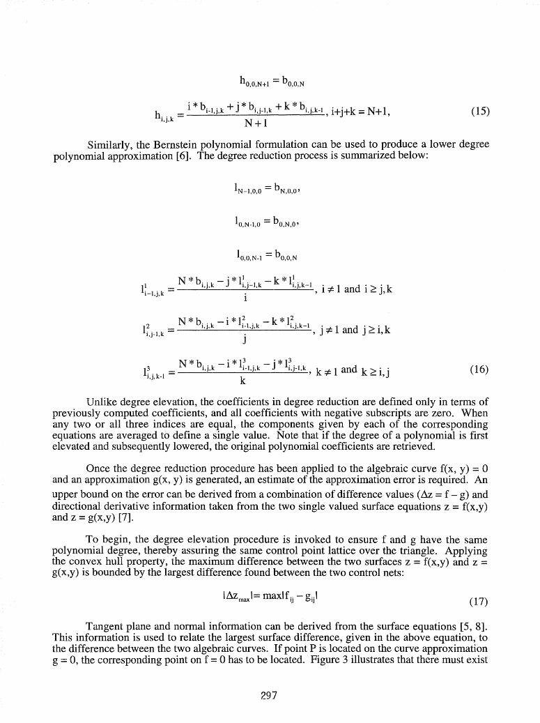
Similarly, the Bernstein polynomial formulation can be used to produce a lower degreepolynomial approximation [6]. The degree reduction process is summarized below:

1 =bN-1,O,O N,O,O'

lo,N-1,o =bo,N,o'

1 =bO,O,N-1 O,O,N

N*l~ 1 . k =--~--~--:.-_---=-1- ,j, i

N*l~ . 1 k =--~---~----"'----

1,]- , j

N*e. k 1. =--~-----.;~--~~l,j, - k

i :;t: 1 and i ~ j, k

j :;t: 1 and j ~ i, k

k:;t: 1 and k ~ i,j (16)

Unlike degree elevation, the coefficients in degree reduction are defined only in terms ofpreviously computed coefficients, and all coefficients with negative subscripts are zero. Whenany two or all three indices are equal, the components given by each of the correspondingequations are averaged to define a single value. Note that if the degree of a polynomial is firstelevated subsequently lowered, the original polynomial coefficients are retrieved.

Once the degree reduction procedure has been applied to the algebraic curve f(x, y) =0and an approximation g(x, y) is generated, an estimate of the approximation error is required. Anupper bound on the error can be derived from a combination of difference values (dz = f g) anddirectional derivative information taken from the two single valued surface equations z = f(x,y)and z =g(x,y) [7].

To begin, the degree elevation procedure is invoked to ensure f and g have the samepolynomial degree, thereby assuring the same control point lattice over the triangle. Applyingthe convex hull property, the maximum difference between the two surfaces z =f(x,y) and z =g(x,y) is bounded by the largest difference found between the two control nets:

(17)

Tangent plane and normal information can be derived from the surface equations [5, 8].This information is used to relate the largest surface difference, given in the above equation, tothe difference between the two algebraic curves. If point P is located on the curve approximationg =0, the corresponding point on f =0 has to be located. Figure 3 illustrates that there must exist

297

........--------1.......... "LlC 9 =0

Figure 3. Error estimation.

s

a point on f = 0 at least within a distance i1C, where S is the smallest angle between the tangent

plane and a direction s defined in the x-y plane, and i1C is given by the equation

i1C = i1ztanS

(18)

Since the surfaces are single valued, tanS defines the value of the directional derivative,

~~, of the function z = f(x,y) with respect to the direction s. If the original Bernstein triangle with

its Bernstein coefficients is called the original patch, then the Bernstein coefficients of thedirectional derivative patch can be calculated from the original patch using the followingequation (for direction s shown in Figure 4):

b.. =N *(B. . 1 - B.. ) ,I,) 1,)+ 1,)

(19)

where i+j <= (N-I) and N is the degree of the original patch.

The convex hull property is applied to the directional derivative patches of f(x,y) and

g(x,y) to determine a minimum value for tanS. Combining the maximum surface difference with

the minimum value of tanS, a single error bound is produced:

(20)

298

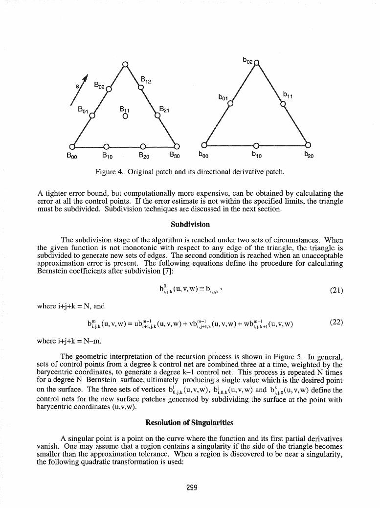
Figure 4. Original patch and its directional derivative patch.

tighter error bound, but computationally more expensive, can be obtained by calculating theerror at the control points. If the error estimate is not within the specified limits, the trianglemust be subdivided. Subdivision techniques are discussed in the next section.

Subdivision

The subdivision stage of the algorithm is reached under two sets of circumstances. Whenthe given function is not monotonic with respect to any edge of the triangle, the triangle issubdivided to generate new sets of edges. The second condition is reached when an unacceptableapproximation error is present. The following equations define the procedure for calculatingBernstein coefficients after subdivision [7]:

where i+j+k =N, and

b?ok(u,v,w)=boOk'l,j, l,j, (21)

where i+j+k =N-m.

(22)

The geometric interpretation of the recursion process is shown in Figure 5. In general,sets of control points from a degree k control net are combinedthree at a time, weighted by thebarycentric coordinates, to generate a degree k-l control neLThisprocess is repeatedN timesfor a degree N Bernstein surface, ultimately producing a single.value which is the desired pointon the surface. The three sets of vertices b~,j,k(u, v,w), bl,o,k(u,v,w) and btj,o(u, v, w) define thecontrol nets for the new surface patches generated by subdividing the surface at the point withbarycentric coordinates (u,v,w).

Resolution of Singularities

A singular point is a point on the curve where the function and its first partial derivativesvanish. One may assume that a region contains a singularity if the side of the triangle becomessmaller than the approximation tolerance. When a region is discovered to be near a singularity,the following quadratic transformation is used:

299

bO1,0,2 bO

2,0,1 bO3,0,0

Figure 5. Subdivision of a bivariate Bernstein polynomial.

x=x

(23)

A piecewise linear approximation is generated near singularities by numerically marchingalong the various branches of the proper transform. The sequence of points generated are thenmapped back to the original coordinate system by reversing the quadratic transformation.

Examples

Examples are presented in this section demonstrating the approximation of a cross­section of a torus using a collection of second degree curves. The curve traces were generatedusing a collection of procedures written in the C programming language and executed on aSun™ SparcStation 2. In each of the examples, approximation is developed over a triangularregion enclosing the closed curve.

The torus used for slicing is centered at (0, 0, 0) and the axis of the torus is straight linegiven by the equation y =x. The radius of the torus is 3, and the radius of the disc rotated aboutthe axis to generate the torus is 0.7.

Figure 6 shows the cross-section of the torus at z =2.2. The number of quadratic curvesegments in this approximation is 306.

300

~ Contours

Figure 6. Torus sliced at z = 2.2.

Figure 7 shows the cross-section of the torus at z =2.3 (the singularity case). The numberof quadratic curve segments in this approximation is 318.

~ Contours

Figure 7. Torus sliced at z =2.3.

Conclusions

-.

This paper discusses a method to directly process Constructive Solid Geometryrepresentations and obtain contour files. Aspects involved in slicing higher degree surfaces, inparticular the torus, are highlighted. The algorithm is applicable to other higher degree surfaces

301

as well, including rational bicubic parametric surfaces. The algorithm provides a rational basisfor approximating geometry for SFF applications.

References

1. Sashidhar, Guduri., Crawford, RichardH. and Beaman, Joseph J., "A Method to '-"V.I..I.V.l.."",V

Exact Contour Files for Solid· Freeform Fabrication", Proceedings of Solid FreeformFabrication Symposium, 1992, Marcus, Harris L., Beaman, Joseph J., Barlow, Joel W.,Bourell, David L., Crawford, Richard H., eds., Austin, TX, August 3-5. pp. 95-101.

2. Waggenspack, Warren N. Jr., Anderson, David C., "Converting Standard BivariatePolynomials to Bernstein Form Over Arbitrary Triangular Regions", Computer AidedDesign, Vol. 18, No 10, 1986. pp 529-532.

3. Waggenspack, Warren N. Jr., Anderson, David C., "Piecewise Parametric Approximationsfor Algebraic Curves", Computer Aided Geometric Design, 1989. 33-53.

4. Abhayankar, Shreeram S. and Bajaj, Chanderjit, "Automatic Rational ofCurves and Surfaces I: Conics and Conicoids", Computer Aided Design, Vol. 19, No 1, 1987.pp 11-14.

5. Farin, Gerald, "Triangular Bernstein-Bezier Patches", Department of Mathematics,University of Utah, Salt Lake City, Utah, USA, 1986.

6. Peterson, Carl S., "Adaptive Contouring of Three-Dimensional Surfaces", Computer AidedGeometric Design, Vol. 1,1984. pp. 61-74.

7. Sederberg, Thomas W., "Planar Piecewise Algebraic Curves", Computer Aided GeometricDesign, Vol. 1, No 4, December 1984. pp 241-255.

8. Farin, Gerald, "Bezier Polynomials Over Triangles and Construction of Piecewise CrPolynomials", Tech Report TRl91 , Department of Mathematics, BruneI University,UxBridge, Middlesex, UK, 1980.

30t'