Direct CPT Methods for Shallow and Deep Foundationsneasce.org/pdf/Conferences/Notes/GEO2019_Paul_Mayne_Direct_CPT... · PPT= Plate Penetration Test PLT= plate load test HPT= Helical

2/13/2019

1

ConeTec Family of Site Investigation Contractors

Proud sponsors of the ASCE G‐I Cross‐USA Lecture Series

Better Information, Better Decisions

Direct CPT Methods for Shallow and Deep Foundations

Paul W. Mayne, PhD, P.E.Georgia Institute of Technology

GeoOmaha 2019 - 36th Annual ConferenceASCE Geo-Institute Cross-USA Lecture SeriesScott Conference Center - 08 February 2019

Reston, VA

2/13/2019

2

Axial Pile Capacity: Qtotal = Qsides + Qbase

Qt

Shaft Capacity

Qs = ∫ fp dAs

Base Capacity

Qb = qb ∙ Ab

unit sidefriction, fp

unit base resistance, qb

Atlanta Hartsfield

Vietnam Port Facility

Ground Surface

Rational Methods for Pile Capacity

End Bearing: qb = pile tip resistance limit plasticity

cavity expansion theory

limit equilibrium

Side Resistance: fp = pile side friction

method: fp = su and = fctn(su)

method: fp = vo' and ≈ K0 tan'

method (offshore)

effective stress methods

numerical simulations (FEM, FD)

2/13/2019

3

ct your privacy, PowerPoint has blocked automatic download of this picture.

SPT

TxPTLPT

VST

PMT

CPMT

DMT

SPLT

K0SB

SWS

HF

BST

TSC

FTS

CPTu

CPT

RCPTu

SCPTu

SDMT

TBPT

BPT

Full Flow PenetrometersSPTT

SCPMTù

SPT = Standard Penetration TestTxPT = Texas Penetration TestVST = Vane Shear TestPMT = Pressuremeter TestCPMT = Cone PressuremeterDMT = Dilatometer TestSPLT = Screw Plate Load TestISB = Iowa K0 Stepped BladeSWS = Swedish Weight SoundingHF = Hydraulic FractureBST = Borehole Shear Test

TSC = Total Stress Cell (spade cell)FTS = Freestand Torsional ShearPV = PiezovaneMPT = Macintosh Probe TestCPT = Cone Penetration TestCPTu = Piezocone PenetrationRCPTu = Resistivity PiezoconeSCPTu = Seismic ConeSDMT = Seismic Flat DilatometerTBPT = T‐Bar Penetrometer TestBPT = Ball PenetrometerTPT = Toroid Penetrometer Test

PPT = Plate Penetration TestPLT = plate load testHPT = Helical Probe TestPBPT = piezoball penetration testRapSochs = Rapid soil characterization systemCPTù = piezodissipation testDMTà = Dilatometer with A‐reading dissipationsSPTT = Standard Penetration Test with TorqueLPT = Large Penetration TestDEPPT = Dual Element PiezoProbe TestHBPT = hemi‐ball penetration testSCPMTu = Seismic Piezocone Pressuremeter

PLT

DEPPTHPT

In‐Situ Geotechnical Test Methods

PPT

MPT

PV PBPT

RapSochs

CPTù

DMTà

TPT HBPT

CONE PENETRATION TEST (CPT): ASTM D 5778

total cone resistance = qt= qc + (1‐anet)∙u2

measured cone resistance = qc

porewater pressure = u2

sleeve friction = fs

inclination = ixy

depth recorder = z

where 0.35 ≤ anet ≤ 0.90 depends on equipment

rods (d = 36mm)in one meterlengths

Constantpush rate of20 mm/s

penetrometer

electronic piezocone

penetrometer

ground surface

readings every1 or 2 seconds

d = 36 mm

rods

electriccable

enlarge

d = 36 mmor 44 mm

ConeTruck(20 tonnes)

2/13/2019

4

Geostratigraphy by CPTu in Portsmouth, Virginia

qt fs u2

CPT• Current Phase Tranformer

• Cross Product Team

• Cellular Paging Teleservice

• Chest Percussion Therapy

• Crisis Planning Team

• Consumer Protection Trends

• Computer Placement Test

• Current Procedural Terminolgy

• Cost Per Treatment

• Choroid Plexus Tumor

• Cardiopulmonary Physical Therapy

• Corrugated Plastic Tubing

• Cumulative Price Threshold

• Cell Prepartion Tube

• Central Payment Tool

• Certified Proctology Technologist

• Cockpit Procedures Trainer

• Color Picture Tube

• Critical Pitting Temperature

• Certified Phelbotomy Technician

• Control Power Transformer

• Cone Penetration Test

• Cost Production Team

• Channel Product Table

• Conditional Probability Table

• Command Post Terminal

2/13/2019

5

Acronyms

APELSCIDLA

Board for: Architects, Professional Engineers, Land Surveyors, Certified Interior Designers and Landscape Architects

DPOR = Dept. of Professional & Occupational Regulation, Commonwealth of Virginia

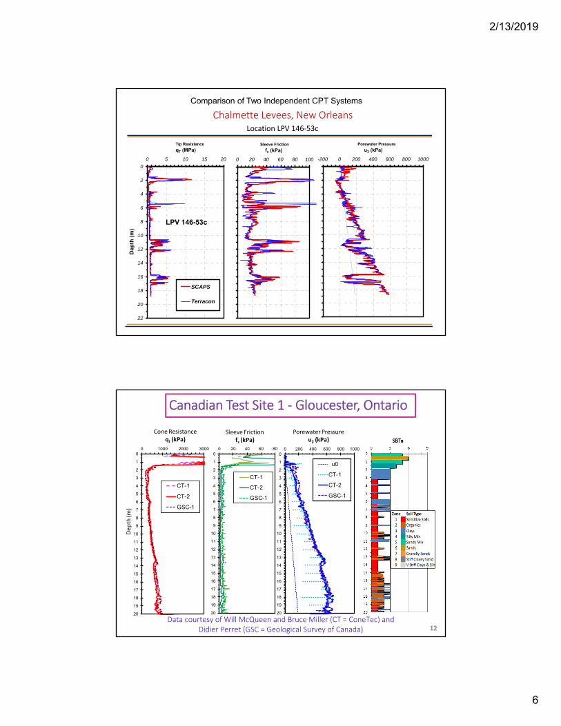
Chalmette Levees, New Orleans

Tip Resistance

0

2

4

6

8

10

12

14

16

18

20

22

0 5 10 15 20

qT (MPa)

Dep

th (

m)

SCAPS

Terracon

Sleeve Friction

0 20 40 60 80 100

fs (kPa)

SCAPS

Terracon

Porewater Pressure

-200 0 200 400 600 800 1000

u2 (kPa)

u0

SCAPS

Terracon

LPV 146-23c

Location LPV 146‐23c

Comparison of Two Independent CPT Systems

2/13/2019

6

Chalmette Levees, New OrleansLocation LPV 146‐53c

Tip Resistance

0

2

4

6

8

10

12

14

16

18

20

22

0 5 10 15 20

qT (MPa)

Dep

th (

m)

SCAPS

Terracon

LPV 146-53c

Sleeve Friction

0 20 40 60 80 100

fs (kPa)Porewater Pressure

-200 0 200 400 600 800 1000

u2 (kPa)

Comparison of Two Independent CPT Systems

Canadian Test Site 1 ‐ Gloucester, Ontario

12

Very sensitive soft clay

0

1

2

3

4

5

6

7

8

9

10

11

12

13

14

15

16

17

18

19

20

0 1000 2000 3000

Depth (m

)

Cone Resistanceqt (kPa)

CT-1

CT-2

GSC-1

0

1

2

3

4

5

6

7

8

9

10

11

12

13

14

15

16

17

18

19

20

0 20 40 60 80

Sleeve Frictionfs (kPa)

CT-1

CT-2

GSC-1

0

1

2

3

4

5

6

7

8

9

10

11

12

13

14

15

16

17

18

19

20

0 200 400 600 800 1000

Porewater Pressureu2 (kPa)

u0

CT-1

CT-2

GSC-1

Data courtesy of Will McQueen and Bruce Miller (CT = ConeTec) and Didier Perret (GSC = Geological Survey of Canada)

2/13/2019

7

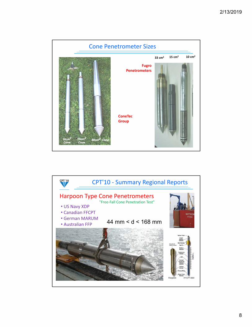
Cone Penetrometers

• 10-cm2

• 15-cm2

• mechanical• electric• cabled• piezo-• electronic• seismic-• digital• wireless

10 cm2 10 cm2 15 cm2 15 cm2

10 cm2

5 cm2

1 cm2

15 cm2

Cone Penetrometer Sizes2 cm2 10 cm2

2/13/2019

8

Cone Penetrometer Sizes

33 cm2 10 cm215 cm2

FugroPenetrometers

ConeTecGroup

CPT'10 ‐ Summary Regional Reports

Harpoon Type Cone Penetrometers

• US Navy XDP• Canadian FFCPT• German MARUM• Australian FFP

"Free‐Fall Cone Penetration Test"

44 mm < d < 168 mm

2/13/2019

9

CPT'10 ‐ Summary Regional Reports

CPT Probes for Centrifuge ‐ Univ. Western Australia

Drum Centrifuge

Main Centrifuge

0 50 mm

T‐bar

Ball

Plate

Mini‐Cone Penetrometers

Micro-Cone PenetrometersKim, Choi, Lee & Lee: Korea University

(GSP GeoFlorida 2010)

FBG = Fibre Bragg Grating sensor

2/13/2019

10

Cone Penetration Rig

Cone Penetration Vehicles

2/13/2019

11

Cone Penetrometer Vehicle

AutoCoson - Robotic CPTby A.P. van den Berg, Holland

PROD = Portable Remotely Operated Drill

by Benthic Geotech Australia

Onshore

Offshore

2/13/2019

12

Cone Penetrometer Testing

Chinese CPT Equipmentwww.madeinchina.com

圆锥贯入试验

Cone Penetrometer Testing

Hand-held electronic cone penetrometers

Rimik CP40

Measured Penetration Resistance

Excellent Repeatability

SpectrumScout SC 900

Eijkelcamp

2/13/2019

13

EarthCPTs

all 7 continents

all 5 oceans

Mars

2/13/2019

14

Launched May 2018Landed November 2018

External Geotechnical Review Team (23 Jan 2013)

MartianPenetrometer

2/13/2019

15

Shear Wave Velocity, Vs• Fundamental measurement in all solids (steel, concrete, wood, soils, rocks)

• Initial stiffness represented by the small‐strain shear modulus (Gdyn = Gmax = G0):

G0 = t Vs2 where total mass density t = t/ga

• Applies to all static & dynamic problems at small strains (s < 10‐6)

• Applicable to both undrained & drained loading cases in geotechnical engineering

Seismic Piezocone Test (SCPTu)Seismic Piezocone Test (SCPTu)Piezocone (CPTu) + Downhole (DHT) = SCPTu

D 7400

Seismic Piezocone Penetration Test

2/13/2019

16

d = 35.7 mm

qt

fs

u2

Vs

Seismic Piezocone Test ‐ Memphis, TN

Meramac River, St. Louis, Missouri

0

2

4

6

8

10

12

14

0 5 10 15 20

De

pth

(m

)

qT (MPa)0 50 100 150 200

fs (kPa)-100 0 100 200 300 400 500

u2 (kPa)0 100 200 300 400

Vs (m/s)

Cone Resistance Sleeve Friction Pore Pressure Shear Wave Velocity

Vs

fs

u2

qt

bad good

200 m/s(656 fps)

5 MPa(50 tsf)

clay sand

2/13/2019

17

CPT Charts for Soil Behavioral Type

Soil Behavioral Type (SBT) charts (Robertson, CGJ, 1990, 1991)

Uses all 3 readings (qt, fs, u2)

Define normalized piezocone parameters:

1. Normalized Tip Resistance: Q = (qt ‐ vo)/vo'

2. Normalized Sleeve Friction (%): F = 100 fs/(qt ‐ vo)

3. Normalized Porewater Pressure: Bq = (u2‐u0)/(qt ‐ vo)

4. Updated Qtn = (qt ‐ vo)/(vo')n where units of atm (≈ tsf)

with n = 1 clay and n = 0.5 in sand (Robertson 2009, 2016)

qt

u2

fs

qt

u2

fs

THIS U2

2/13/2019

18

Soil Behavioral Type Using CPT Index, Ic• Use of CPT Material Index (Ic) for identification of soil type (Robertson & Wride, 1998):

• Modified normalized tip resistance (Robertson 2004):

• Exponent n = 0.5 (sands), 0.75 (silts), n = 1.0 (clays)

• Iterate to find exponent n (Robertson 2009 CGJ):

22 )log22.1()log47.3( FQIc

n

vo

atm

atm

vottn

qQQ

'

)(

0.115.0)/'(05.0381.0 atmvocIn

sands: Ic < 2.05clays: Ic > 2.95

( ):

( ')t vo

tn nvo

qbars Q

1

10

100

1000

0.1 1 10

Nor

mal

ized

Con

e R

esis

tanc

e, Q

tn

Friction Ratio, Fr = 100 fst/(qt - vo) (%)

CPT Soil Behavioral Type Chart (Robertson 2009)

Sensitive Soils(Zone 1)

StiffclayeySand

(Zone 8)

VeryStiffclaysandsilts

(Zone 9)

22 )log22.1()log47.3( FQIc

2/13/2019

19

CPTu in Nebraska: Courtesy: Bruce Miller, ConeTec0 3 6 9

Soil BehavioralType (SBTn) Chartfor normalized CPT

(after Robertson 2009)

1

10

100

1000

0.1 1 10

Nor

mal

ized

Tip

Res

ista

nce

, Q

tn

Normalized Friction, Fr = 100 fs /(qt - vo) (%)

9 - ZONE SBT

Gravelly Sands (zone 7)

Sands(zone 6)

Sandy Mixtures(zone 5)

Silt Mix(zone 4)

Clays(zone 3)

Organic Soils(zone 2)

FocalPoint

Sensitive Claysand Silts(zone 1)

Ic = 1.31

Ic = 2.05

Ic = 2.60

Ic = 2.95

Ic = 3.60

Notes:

Ic = Radius:

Very stiff OC clayto silt (zone 9)

natmvo

atmvottn

qQ

)/'(

/)(

22 )log22.1()log47.3( rtnc FQI

Very stiffOC sandto clayey

sand(zone 8)

Exponent: 15.0)/'(05.0381.0 atmvocIn

a. Find sensitive soils of zone 1 identified when: Qtn < 12 exp(-1.4 Fr )

b. Identify: Zone 8 (1.5 < Fr< 4.5%) and Zone 9 (Fr > 4.5%):

c. Use CPT index Ic for Zones 2 through 7 002.0)9.0(0004.0)9.0(006.0

12

rr

tn FFQ

ApproximateAlgorithm Steps:

Ic < 2.6: Drained

Ic > 2.6: Undrained

2/13/2019

20

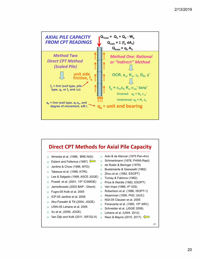
Undrained: qb = Nc su

Qside = (fp dAs)

QTotal = Qs + Qb - Wp

fp = cmck Ko vo’ tan’

Qbase = qb Ab

Drained: qb = Nq vo’

Method One: Rational or “Indirect” Method

AXIAL PILE CAPACITY FROM CPT READINGS

qb = unit end bearing

unit sidefriction, fp

Method TwoDirect CPT Method

(Scaled Pile)

fp = fctn (soil type, piletype, qt, or fs and u)

qb = fctn (soil type, qt-ub, and degree of movement, s/B )

OCR, su, Ko, t, DR, ’

Aoki & de Alencar (1975 Pan-Am)

Schmertmann (1978, FHWA Rept)

de Ruiter & Beringer (1979)

Bustamante & Gianeselli (1982)

Zhou et al. (1982, ESOPT)

Tumay & Fakhroo (1982)

Price & Wardle (1982, ESOPT)

Van Impe (1986, 4th IGS)

Robertson et al. (1988, ISOPT-1)

Alsamman (1995, PhD, UIUC)

NGI-05 Clausen et al. 2005

Fioravante et al. (1995, 10th ARC)

Schneider et al. (JGGE 2008)

Lehane et al. (UWA 2012)

Niazi & Mayne (2015, 2017)

Almeida et al. (1996, BRE-NGI)

Eslami and Fellenius (1997)

Jardine & Chow (1996, MTD)

Takesue et al. (1998, KTRI)

Lee & Salgado (1999, ASCE JGGE)

Powell, et al. (2001, 15th ICSMGE)

Jamiolkowski (2003 BAP - Ghent)

Fugro-05 Kolk et al. 2005

ICP-05 Jardine et al. 2005

Abu-Farsakh & Titi (2004, JGGE)

UWA-05 Lehane et al. 2005

Xu et al. (2006, JGGE)

Van Dijk and Kolk (2011, ISFOG-II)

40

Direct CPT Methods for Axial Pile Capacity

2/13/2019

21

Unicone CPTu Method

Soil Type Cse Value

1. Very soft sensitive soils 0.080

2. Soft Clay 0.050

3. Stiff clay to silty clay 0.025

4. Silt-Sand Mix 0.010

5. Sands 0.004

Eslami & Fellenius (1997) Canadian Geot. J.www.fellenius.net

A. Determineeffective coneresistance:qE = qt ‐ u2

B. Plot qE vs fs for soil type (zones 1 to 5)

C. Unit Side Resistance: fp = Cse∙qE

D. Unit Tip Resistance:qb = Cte∙qE

B < 0.4m: Cte = 1B > 0.4m: Cte = 1/(3B)B = pile width (m)

0.1

1

10

100

1 10 100 1000

Sleeve Friction, fs (kPa)

q E =

qt-

u 2 (

MPa

)1- Very soft clays, sensitive soils2- Soft clays3- Silty clays - Stiff clays4- Silty sands - Sandy silts5- Sands, Gravelly Sands

21

3

4

5

Summaryof 40

availabledirect CPTmethods

2/13/2019

22

www.mapcruzin.com

North America (40 Sites)

Canada: 11 Sites USA: 28 Sites Puerto Rico: 1 Site

Overview330 pile load tests

70 sites19 countries

China: 2 Iraq: 1 Japan: 2

Malaysia: 1 Thailand: 1

Asia (7 Sites)

Enhanced Unicone Method (Niazi & Mayne 2016)Enhanced Unicone Method (Niazi & Mayne 2016)

Europe (21 Sites)

Belgium: 2 France: 4 Ireland: 3 Netherlands: 2

Norway: 2 Portugal: 1 United Kingdom: 7

CPT SoundingsSCPT/SCPTu: 59

CPTu: 9CPT: 4

Unicone Method (1997): 102 load tests

Enhanced Unicone(2016): 330 load tests

Cse = Cse(mean) ∙ PileType ∙ t-c ∙ rate

Enhanced Unicone: Pile Side Friction: fp = Cse∙qE

Compression: t-c = 1.11 Tension/Uplift: t-c = 0.85

Bored Piles: PileType = 0.84 Jacked Piles: PileType = 1.02 Driven Piles: PileType = 1.13

Pile Type:

CRP: rate = 1.09 MLT: rate = 0.97

Direction of Loading: Rate of Loading:CRP = constant rate

of penetrationMLT = maintained load test

)605.3732.0()( 10 cI

meanseCSIDE FRICTION

Pile End Bearing Resistance: qb = Cte(mean)∙qE

)218.1325.0()( 10 cI

meanteC

2/13/2019

23

Pile end-bearing resistance in sands

Randolph (Lovell Lecture, Purdue University)

Randolph (2003 Rankine Lecture, Geotechnique)

For Ic < 2.6: Pile End Bearing Resistance: qb = toeCte∙qE

toe

w/d = Normalized Displacement

Various Axial Pile Capacity Criteria(Mayne 2009, IFCEE, Orlando)

GT Drilled Shaft C2d = 0.76 m; L = 16.9 m

0

1000

2000

3000

4000

5000

6000

0 50 100 150 200Displacement, wt (mm)

Ap

plie

d L

oad

, Q (

kN)

DeBeer (2231 kN)VanDer Veen (2667)

Davisson Offset Line (2773)Mazurkiewicz (2782)

Butler & Hoy(3289 kN)

Brinch Hansen 90% criterion (3334)

Brinch HansenParabola (3467)

Fuller &Hoy (4178)

Chin-Kondner Criterion:Hyperbolic Asymptote (5103)

LCPC: s/B = 10% criterion (3821 kN)

Hirany & Kulhawy(3155 kN)

2/13/2019

24

Soil Es and v constant with depth

Side Load, Ps

s

tt Ed

IPw

Load Transfer to Base:

)]1)(/(5ln[

)/(

)1(1

11

2 vdL

dLI

21

I

P

P

t

bBase Load, Pb

RIGID PILE RESPONSE

Ground Surface

Pt = Ps + Pb = Total LoadRandolph Model

d = diameterL = Length

Top Displacement, wt

Axial Pile Displacement Influence Factor, I0

Randolph & Wroth (1979); Poulos & Davis (1980)

Rigid Pile in an Infinite Elastic Medium

0.01

0.10

1.00

0 10 20 30 40 50 60 70 80 90 100

Slenderness Ratio, L/d

Infl

uen

ce F

act

or,

I o

Boundary Elements

Closed Form v = 0.5

Closed Form v = 0.2

Closed Form v = 0

s

ott Ed

IPw

Poulos & Davis (1980) vs. Randolph SolutionForcePt

SoilModulusEs

d = pilediameter

L = pilelength

wt

2/13/2019

25

Soil Modulus for Monotonic Load Response

Gmax = t Vs2

t = t/g

Emax = 2Gmax(1+)

Modulus Reduction from TS and TX Data

0

0.1

0.2

0.3

0.4

0.5

0.6

0.7

0.8

0.9

1

0 0.1 0.2 0.3 0.4 0.5 0.6 0.7 0.8 0.9 1

Mobilized Strength, /max or q/qmax

Mo

du

lus

Red

uct

ion

, G/G

max

or

E/E

max

NC S.L.B. Sand

OC S.L.B. Sand

Hamaoka Sand

Hamaoka Sand

Toyoura Sand e = 0.67

Toyoura Sand e = 0.83

Ham River Sand

Ticino Sand

Kentucky Clayey Sand

Kaolin

Kiyohoro Silty Clay

Pisa Clay

Fujinomori Clay

Pietrafitta Clay

Thanet Clay

London Clay

Vallericca Clay

= 1/FS

Open = DrainedClosed = Undrained

(TS = torsional shear; TX = triaxial shear)

FS = factor of safetyE = 2G(1+)

2/13/2019

26

Modulus Reduction Scheme (Fahey & Carter 1993)

0

0.1

0.2

0.3

0.4

0.5

0.6

0.7

0.8

0.9

1

0 0.1 0.2 0.3 0.4 0.5 0.6 0.7 0.8 0.9 1

Mobilized Stress Level, q/qmax

Mo

du

lus

Red

uct

ion

, E

/Em

ax

g = 1.0

g = 0.4

g = 0.3

g = 0.2

Note: f = 1

gqqfEE )/(1/ maxmax

Operational modulus: E = (E/Emax)ꞏEmax

E = 2G(1+)

= 1/FS

V

Qsu = (fp dAs)

Qtu = Qs + Qb

Qbu = qb Ab

fp = fctn (qt-u2 and Ic)

RIGID PILE RESPONSE

qb = unit end bearing

unit side friction, fp

CPT

qt

u2

fs

Vs Emax = 2 t Vs2 (1+)

Top Displacement, wt

])/(1[ 3.0max tut

tt

QQEd

IQw

Load Transfer

)]1)(/(5ln[

)/(

)1(1

11

2 vdL

dLI

21

I

Q

Q

t

bqb = fctn (qt-u2 and Ic)

2/13/2019

27

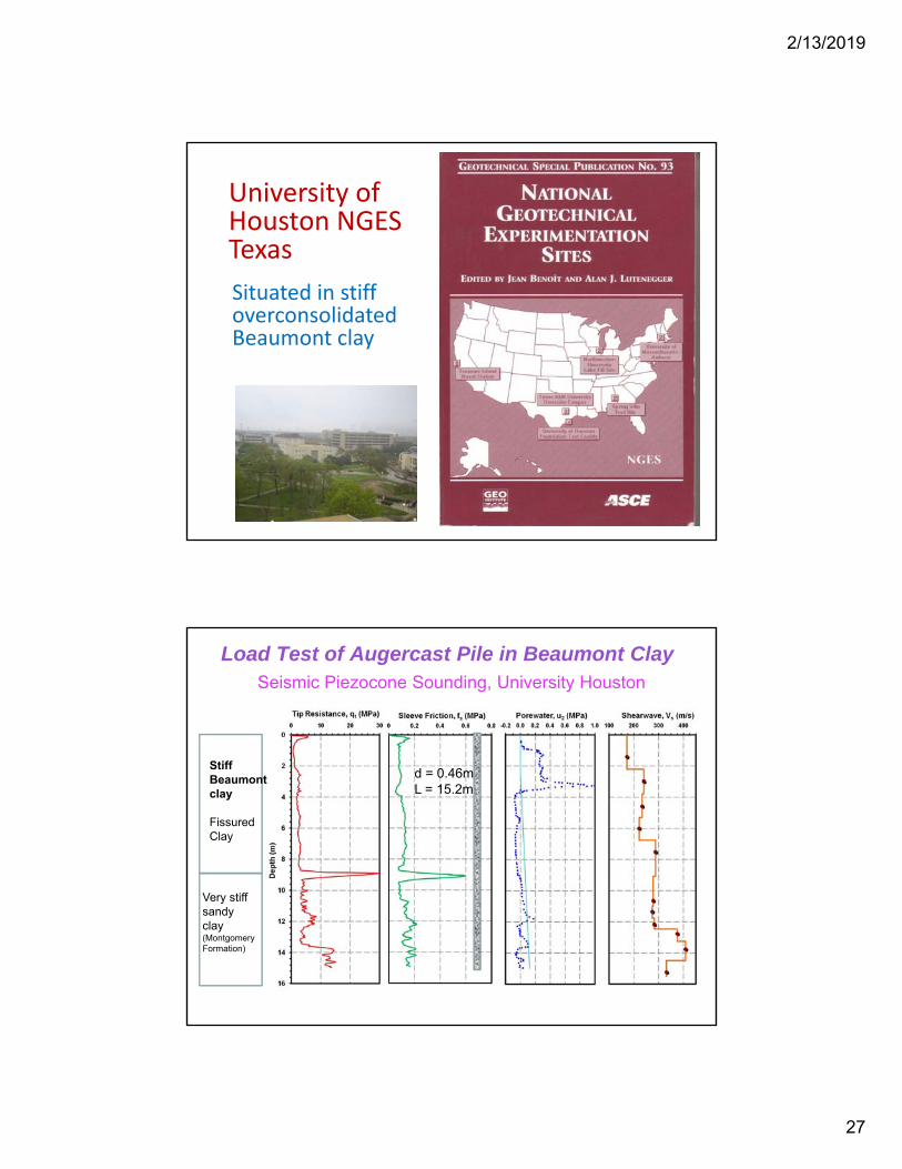
University of Houston NGESTexas

Situated in stiff overconsolidatedBeaumont clay

Seismic Piezocone Sounding, University Houston

Load Test of Augercast Pile in Beaumont Clay

StiffBeaumontclay

FissuredClay

Very stiffsandyclay(MontgomeryFormation)

d = 0.46mL = 15.2m

2/13/2019

28

Auger Cast-in-place Piles at Univ. Houston

ACIP Pile, University of Houston Input Parameters

Length L= 15.20 m = 0.50Diam. d = 0.456 m I = 0.058Emax = 363,855 kPa Qcap. = 1800 kN

Q/Qult = 1/FS E/Emax Qt (kN) Qb (kN) Qs (kN) E (kPa) s (m) s (mm)

0.00 1.00 0 0 0 363,855 0.000 0.000.02 0.69 36 3 33 251,333 0.000 0.020.05 0.59 90 7 83 215,733 0.000 0.050.10 0.50 180 14 166 181,495 0.000 0.130.15 0.43 270 21 249 157,908 0.000 0.220.20 0.38 360 28 332 139,344 0.000 0.330.30 0.30 540 42 498 110,304 0.001 0.630.40 0.24 720 56 664 87,450 0.001 1.050.50 0.19 900 70 830 68,313 0.002 1.690.60 0.14 1,080 84 996 51,697 0.003 2.680.70 0.10 1,260 98 1,162 36,923 0.004 4.370.80 0.06 1,440 112 1,328 23,560 0.008 7.830.90 0.03 1,620 126 1,494 11,321 0.018 18.330.98 0.01 1,764 137 1,627 2,199 0.103 102.79

)]1)(/(5ln[

)/(

)1(1

11

2 vdL

dLI

21

I

Q

Q

t

b

s

pt

Ed

IQs

Elastic Influence Factor:

Pile Displacements:

Load Transfer:

Elastic Continuum Pile Solution

(O'Neill, 2000)

ACIP Concrete Piles at UH (O'Neill, 2000)

Rigid Elastic Pile Solution

0

10

20

30

40

50

60

0 200 400 600 800 1000 1200 1400 1600 1800 2000

Axial Load, Q (kN)

To

p D

efl

ec

tio

n (

mm

)

Qtotal = Qs + QbPredicted QbPredicted QsMeasured TotalMeasured ShaftMeasured Base

2/13/2019

29

SCPTu at Texas A&M Sand Site(Tumay & Bynoe 1998)

Tip Resistance

0

2

4

6

8

10

12

14

16

0 10 20 30

qT (MPa)

Dep

th (

m)

Sleeve Friction

0 100 200 300 400

fs (kPa)

Pore Water Pressure

-200 0 200 400 600

u1 (kPa)Shear Wave velocity

0 100 200 300 400 500

Vs (m/s)

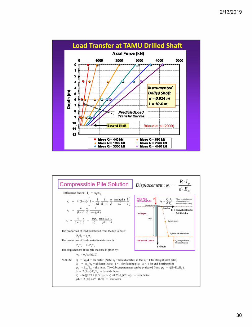
SANDS

Drilled Shaft at Texas A&M Sand Site(Briaud et al. 2000 ‐ Journal Geot. & Geoenv. Engrg)

0

10

20

30

40

50

60

70

80

0 1000 2000 3000 4000 5000

Axial Load, Q (kN)

Top

Def

lect

ion,

wt

(mm)

Pred. Qt Pred. Qs Pred. Qb

Measured Total Measured Shaft Measured Base

Axial Load Q (kN)

Displacemen

t, w

t(m

m)

d = 0.914 mL = 10.4 m

2/13/2019

30

Load Transfer at TAMU Drilled Shaft

Briaud et al (2000)

Compressible Pile SolutionsL

ptt Ed

IPwntDisplaceme

:

d

L

L

Lx

)tanh(

)1(

811)1(41

d

L

L

Lx E

)tanh(4

)1(

43

Influence factor: Ip = x1/x3

The proportion of load transferred from the top to base:

Pb/Pt = x2/x3

The proportion of load carried in side shear is:

Ps/Pt = 1 - Pb/Pt

The displacement at the pile toe/base is given by:

wb = wt/cosh(L)

NOTES: = db/d = eta factor (Note: db = base diameter, so that = 1 for straight shaft piles) = EsL/Eb = xi factor (Note: = 1 for floating pile; < 1 for end-bearing pile)E = Esm/EsL = rho term. The Gibson parameter can be evaluated from: E = ½(1+Es0/EsL). = 2(1+)Ep/EsL = lambda factor = ln{[0.25 + (2.5 E(1- ) - 0.25)] (2L/d)} = zeta factorL = 2(2/)0.5 (L/d) = mu factor

)cosh(

1

)1(

42 L

x

Es = Equivalent ElasticSoil Modulus

AXIAL PILEDISPLACEMENTS

LengthL

Diameter dEso(surface)

EsM (mid-length)

EsL (along side at tip/toe/base)

Eb (base geomaterialModulus of layer 2)

sL

tt Ed

IPw

Pt Where Ip = displacementInfluence factor fromelastic continuum theory

z = Depth

Soil Layer 1

Soil or Rock Layer 2

2/13/2019

31

I-85 Bridge, Coweta County, Georgia

Drilled Shaft Load Test: d = 0.914 m; L = 20.1 m

SCPTu at I-85, Newnan, GACourtesy: Dr. Alec McGillivray

0

2

4

6

8

10

12

14

16

18

0 2 4 6 8

qT (MPa)

De

pth

(m

)

0

2

4

6

8

10

12

14

16

18

0 100 200 300

fs (kPa) Ub (kPa)

0

2

4

6

8

10

12

14

16

18

-100 0 100 200

0

2

4

6

8

10

12

14

16

18

0 100 200 300 400

Vs (m/s)

2/13/2019

32

Axial Load Response of I‐85 Drilled Shaft

Qt

Qs

Qb

Class “A” Prediction of Axial Pile ResponseJackson County, Georgia

Driven 273 mm diameter closed‐ended steel pipe piles; 8 < L < 18 m.

CPT qt, fs and u2 used for axial capacity

Shear wave Vs provides initial stiffness

Turbine Foundations,Plant Dahlberg Power StationSouthern Companies

2/13/2019

33

Axial Pile Response from SCPTu, Jackson County, GA

Residual soils of the Atlantic Piedmont Geology


Driven Steel Pipe Pile No. P22 (L = 9.45 m)

0

2

4

6

8

10

12

14

0 200 400 600 800 1000 1200

Axial Load, Q (kN)

Def

lect

ion,

w t

(m

m)

Predicted by SCPTuin Advance

Measured

2/13/2019

34


Driven Steel Pipe Pile No. P33 (L = 17.8 m)

0

2

4

6

8

10

12

14

0 200 400 600 800 1000 1200

Axial Load, Q (kN)Def

lect

ion,

w t

(m

m)

Predicted in advance from SCPTU data

Measured from Load Test

New Movie

Carson ‐ the black lab mix

Georgia LabRescue (2005)

puppy

2/13/2019

35

MY DOG

Carson Mayne

Black Lab Mix

Now 13 years old

His walking is limited

Gets long‐winded

Tires easily

2/13/2019

36

New Movie

72

www.hindu.com www2.dot.ca.gov

www.statnamiceurope.com

Reaction FrameDead Weight

Osterberg CellStatnamic Load Testwww.fhwa.dot.gov

Pile Load Tests

2/13/2019

37

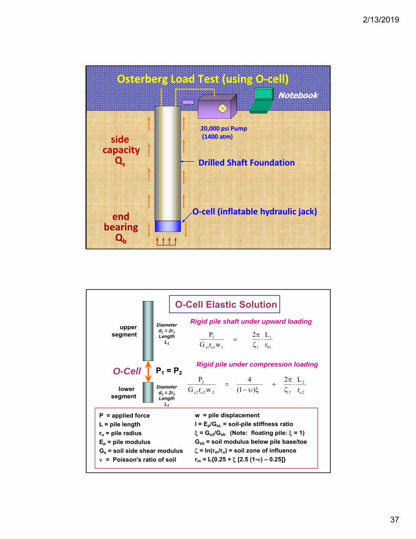
Osterberg Load Test (using O‐cell)

O‐cell (inflatable hydraulic jack)

Drilled Shaft Foundation

Notebook

20,000 psi Pump(1400 atm)side

capacityQs

end bearing

Qb

O-Cell Elastic Solution

01

1

111o1s

1

r

L2

wrG

P

P = applied force

L = pile length

ro = pile radius

Ep = pile modulus

Gs = soil side shear modulus

= Poisson's ratio of soil

2o

2

222o2s

2

r

L2

)1(

4

wrG

P

Rigid pile under compression loading

Rigid pile shaft under upward loadingupper

segment

lower segment

O-Cell

w = pile displacement

l = Ep/GsL = soil-pile stiffness ratio

= Gs2/Gsb (Note: floating pile: = 1)

Gsb = soil modulus below pile base/toe

= ln(rm/ro) = soil zone of influence

rm = L{0.25 + [2.5 (1-) – 0.25]}

P1 = P2

Diameterd1 = 2r1

LengthL1

Diameterd2 = 2r2

LengthL2

2/13/2019

38

Calgary Drilled Shaft O-Cell Load Test by Seismic Piezocone Tests

CPT05-13 Calgary

0

2

4

6

8

10

12

14

16

18

20

22

24

0 10000 20000

Tip Stress, qt (kPa)

Dep

th (met

ers)

0 200 400 600

Sleeve Friction, fS (kPa)-500 0 500 1000

Porewater, u2 (kPa)

u2

uo-hydro

0 100 200 300 400 500 600

Shear Wave, VS (m/s)

DrilledShaft O-CellLoad Test

Dimensionsd = 1.4 mL = 14 m

O-Cell

Evaluation of Calgary O-Cell Shaft Response by Seismic Piezocone Tests

Calgary Foothills Medical Center O-cell load test data App. A, page 3 of 5

O-Cell Load Test Results LOADTEST Project No. LOT-9121 (Figure 1)

-40

-30

-20

-10

0

10

20

30

40

50

60

70

80

0 1000 2000 3000 4000 5000 6000 7000 8000

O-Cell Load, Q (kN)

Displac

emen

t, w

(mm)

Loading Down Measured Below O-Cell

Measured Above O-Cell Loading Up

d = 1.4 m

L = 10 m

L = 4 m

2/13/2019

39

Cooper River Bridge, Charleston, SC

Deep Foundations: 2.5 m‐ and 3‐m diameterdrilled shafts with lengths of 45 to 60 m

Arthur Ravenel Bridge over Cooper River, SC

0

10

20

30

40

50

60

0 5 10 15 20Tip Stress, qt (MPa)

Dep

th (

m)

0 50 100 150

Sleeve, fs (kPa)

0 1 2 3 4 5

Porewater, ub (MPa)

0 100 200 300 400 500 600

Shear Wave, Vs (m/s)

Mean of 5nearbySCPTs

SCPTu 31

(Camp, ASCE GeoSupport GSP 2004)

2/13/2019

40

-150

-100

-50

0

50

100

0 10 20 30 40

O-Cell Load, Q (MN)

Displac

emen

t, w

(mm)

Meas. Stage 1 Lower O-Cell: Load Down

Meas. Stage 2 Upper O-Cell: Load Down

Meas. Stage 3 Upper O-Cell: Load Up

Shaft diameter d = 2.6 m

L = 16.3 m

L = 2.5 m

L = 14.2 m

L = 14.0 m

1 m

1

2

3UpperO-Cell

LowerO-Cell

Casing

10 m

20 m

30 m

40 m

0 m Depth

48 m

Arthur Ravenel BridgeCooper River, Charleston, SC

Input Parameters for Plaxis FEM(Schweiger 2012): Hardening Soil Small Model

Input from SCPTu√ SBT or fs√ Vs or fs√ qt1

√ NTH Nm

√ qt1

' = 0.2; u = 0.5√ Vs and Qtn

√ Ic and Qtn

√ Vs and Qtn

√ Icatm = 100 kPa√ qt, OCR, '‐‐√ Vs

‐

2/13/2019

41

qt = cone resistance → qnet = qt ‐ vo

fs = sleeve frictionu2 = porewater pressure

qfooting = stress

Direct CPT ApproachConventional Approach

Bearing Capacity Settlements CPT

Limit Plasticity

ElasticContinuum

Theory

B B B

III

IIIII

III z

footing

s = displacement

qult = bearing capacityt = unit weight' = friction anglesu = undrained strengthc' = effective cohesion interceptNc = cohesion bearing factorN = unit weight bearing factorNq = surcharge bearing factor

s = displacement = Poisson's ratioE' = Young's modulusD' = constrained modulusEu = undrained modulusp' = preconsolidationIGHFE = elasticity factors

)/( Bsqhq netsfooting

soil type

qvocult NNBcNq '21

E

IBqs GHFE )1( 2

Evaluating Shallow Foundation Response from CPT

Direct CPT Method for FootingsMayne and Illingworth (2010, ASCE GeoCongress)

2/13/2019

42

Direct CPT Method for Spread Footings on Sands

• A Database Approach using CPT

• 32 Large Footings (0.5 m < B < 6 m)

• 13 Sand Sites ‐ clean to slightly silty Sands

• All sites tested by CPT

• Characteristic Load‐Displacement Curve: Fellenius (1994); Briaud & Gibbens (1994); Lutenegger & Adams (1998, 2003); Briaud (2007)

• Stress (q) vs. normalized displacement (s/B)

Direct CPT Method for Spread FootingsCharacteristic Stress‐Normalized Displacement Curves

Fittja, Sweden

0.0

0.5

1.0

1.5

2.0

2.5

0 20 40 60 80 100

Displacement, s (mm)

App

lied

Load

, Q

(M

N) 2.5 m x 2.3m

1.8 x 1.6m

0.65m 0.55m

2/13/2019

43


Fittja, Sweden

0.0

0.1

0.2

0.3

0.4

0.5

0.6

0.7

0.8

0.9

1.0

0.00 0.05 0.10 0.15

Normalized Displacement, s/B

App

lied

Str

ess,

q (

MP

a) 2.5 m x 2.3m

1.8 x 1.6m

0.65m 0.55m


Fittja, Sweden

0.0

0.5

1.0

1.5

0.0 0.1 0.2 0.3 0.4 0.5

Square Root (s/B)

Ap

plie

d S

tres

s, q

(M

Pa) 0.55 x 0.65 m

1.6 x 1.8 m

2.3 x 2.5 m

Regression:n = 21

q = 2.03 sqrt(s/B)

r2 = 0.980rs = 2.03 MPa

2/13/2019

44


Texas A&M Footings (Briaud & Gibbens, 1994, GSP 41)

0

1

2

3

4

5

6

7

8

9

10

11

12

0 20 40 60 80 100 120 140 160 180


Ap

plie

d L

oad

, Q (

MN

)

3m N

3m S

2.5 m

1.5 m

1.0 m

Square Footings: B (meters) =3

3

2.5

1.5

1.0

2014 Direct CPT Method for Footings on Sand

2/13/2019

45

Shenton Park sand site, Perth, Australia

CPTs from Shenton Park, Perth, Australia

2/13/2019

46



2/13/2019

47


Database: 32 Large Footings on 13 Sands

Sand Site Location Soil Conditions Footings: Numbers, Reference/Source

Shapes, and Sizes

College Station Texas Deltaic sand 5 Square: 1, 1.5, 2.5, 3 m Briaud & Gibbens (1999, JGE)

Kolbyttemon Sweden Glaciofluvial sand 4 Rect: B = 0.6; 1.2, 1.7, 2.4 m Bergdahl, et al. (1985 ICSMFE)

Fittja Sweden Glaciofluvial sand 3 Rect: B=0.6m, 1.7, 2.4 m Bergdahl, et al. (1985 ICSMFE)

Alvin West Texas Alluvial sand 2 Circular: D = 2.35 m Tand, et al. (1994, GSP 40)

Alvin East Texas Alluvial sand 2 Circular: D = 2.2 m Tand, et al. (1994, GSP 40)

Perth Australia Siliceous dune sand 4 Square: B = 0.5 and 1.0 m Lehane (2008, 4th DCG)

Grabo T1C Sweden Compacted sand fill 1 Square: B = 0.46 m Phunc duc Long (1993, SGI 43)



Labenne France Aeolian Dune sand 4 Square: B = 0.7 and 1.0 m Amar et al. (1998, ISC-1)

Green Cove Florida Marine silty sand 1 Circular: D = 1.82 m Anderson et al. (2006, JGGE)

Durbin South Africa Alluvial fine sand 1 Square: B = 6.09 m Kantley (1965, ICSMFE)

Porto Portugal Residual silty sand 2 circles: D = 0.53 and 1.1 m Viana da Fonseca (2001, JGGE)

Limit Plasticity

Active

Qult

Radial

Passive

Elasticity Theory

diameter d

d

2d

1.5d

Depth of Influence

2/13/2019

48


0.0

0.2

0.4

0.6

0.8

1.0

1.2

1.4

1.6

1.8

2.0

0.0 0.1 0.2 0.3 0.4 0.5 0.6

Sqrt Normalized Displacement, (s/B)0.5

Fo

otin

g S

tres

s, q

app

lied

(MP

a)

qc = 10.72 Kolbyttemon

qc = 10.46 Alvin West

qc = 9.78 Green Cove

qc = 7.52 Texas A&M

qc = 6.72 Alvin East

qc = 4.01 Labenne

qc = 3.21 Fittja

qc = 3.66 Durbin

qc = 3.86 Grabo T2C

qc = 2.87 Grabo T3C

qc = 3.44 Perth

qc = 0.88 Grabo T1C

Summary: 30 Footings on 12 Sand Sites

/ ( /s footingr q s B


0.00

0.05

0.10

0.15

0.20

0.25

0.30

0.0 0.1 0.2 0.3 0.4 0.5 0.6

Nor

mal

ized

Str

ess,

q a

pp

lied

/qc


Footing Response on Sands

Alvin East, Texas

Alvin West, Texas

Durbin, South Africa

Fittja, Sweden

Grabo T1C

Grabo T2C

Grabo T3C

Green Cove, Florida

Kolbyttemon, Sweden

Labenne, France

Perth, Australia

Porto, Portugal

Texas A&M

Regression

32 Footingson 13 Sandsn = 376r2 = 0.933S.E.Y. = 0.0143

q/qc = 0.585 (s/B)0.5

2/13/2019

49

Footings on Sand ‐ Interpretation

0

100

200

300

400

500

600

700

800

900

1000

1100

1200

0 20 40 60 80 100 120

App

lied

Axi

al L

oad,

Q

(kN)


Labenne Footing, France

What is the bearing capacity?

B = 1.0 m

Footings on Sand by CPT

0

100

200

300

400

500

600

700

800

900

1000

1100

1200

0 20 40 60 80 100 120

App

lied

Axi

al L

oad,

Q

(kN)


Labenne Footing, France

What is the bearing capacity?

LCPC criterion:Q when (s/B) = 10%

B = 1.0 m

s = 100 mm

Qcap = 870 kN

Capacity Criteria: LCPC (Amar 1998)

2/13/2019

50

Bearing Capacity Evaluation - Texas A&M Footings

y = 0.5935xR² = 0.9274

0.0

0.1

0.2

0.3

0.4

0.5

0.0 0.1 0.2 0.3 0.4 0.5 0.6

No

rma

lize

d S

tre

ss, p

F /q

c


Footing Response on Sands

32 Footings on Mainly Quartz and Silica Sands

8 Footings on Calcareous Sand

Euro Capacity at s/B = 10%or (s/B)0.5 = 0.316

︶B/s︵q58.0p cF

Response of 40 Footing Load Tests on SandsClean Quartz Sands: pult ≈ 0.18 qc

pult = 0.18 qc

2/13/2019

51

Direct CPT Method for Footing Response on Soils

Database approach:

• 74 footings (80% square; 20% circular)

• Large dimensions: 0.5 m < B < 6m +

• 40 spread footings on 14 sands

• 10 footings on 4 silts

• 14 footings or plates on 6 intact clays

• 10 large plates on 6 fissured clays

Mayne and Woeller (2014, ASCE GeoCongress, Atlanta)

2012 Direct CPT Method for Footings on SoilsFooting Response on Clays, Silts,& Sands

0.0

0.1

0.2

0.3

0.4

0.5

0.6

0.7

0.8

0.9

1.0

0.0 0.1 0.2 0.3 0.4 0.5 0.6


Nor

ma

lize

d S

tres

s, q

ap

plie

d /

q tn

et

Intact ClaysFissured ClaysSiltsSands

)B/s(qh)stress(q tnets

Intact Clays: hs = 2.70

Fissured: hs = 1.47

Sands: hs = 0.58

Silts: hs = 1.12

2/13/2019

52

2014 Direct CPT Method for Footings on Soils

Footing Response on Clays, Silts,& Sands

0.001

0.01

0.1

1

10

0.001 0.01 0.1 1 10

Predicted stress, q (MPa)

App

lied

stre

ss,

q (M

Pa)

Clays: hs = 2.70Fissured: hs = 1.47Silts: hs = 1.12Sands: hs = 0.58

For Sands & Silts: Limit: s/B < 0.1For Clays: Limit: s/B < 0.04

All datan = 659

Regressions:1. Arithmetic: y = 1.005 x

r2 = 0.9372. Log-Log

y = 1.044x1.02

r2 = 0.926

)B/s(qh)stress(q tnets

2014 Direct CPT Method for Footings on Soils

Footing Response on Clays, Silts,& Sands

y = 1.0038x

R2 = 0.9473

y = 1.0045x

R2 = 0.8807

y = 1.0037x

R2 = 0.9248

y = 1.0265x

R2 = 0.9348

0.0

0.5

1.0

1.5

2.0

2.5

0.0 0.5 1.0 1.5 2.0 2.5

Predicted stress, q (MPa)

App

lied

stre

ss,

q (M

Pa)

Sands

Silts

Clays

Fissured

Sands & Silts: s/B < 0.1For Clays: s/B < 0.04

Sands:

Silts:

IntactClays:

Fissured Clays:

2/13/2019

53

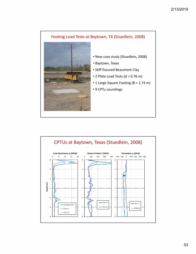
• New case study (Stuedlein, 2008)

• Baytown, Texas

• Stiff fissured Beaumont Clay

• 2 Plate Load Tests (d = 0.76 m)

• 1 Large Square Footing (B = 2.74 m)

• 9 CPTu soundings

Footing Load Tests at Baytown, TX (Stuedlein, 2008)

CPTUs at Baytown, Texas (Stuedlein, 2008)

2/13/2019

54


0

1000

2000

3000

4000

0 50 100 150 200

Footing Load

, Q (kN

)


Plate P30‐1

Plate P30‐2

Footing P‐G3

Direct CPT (B = 2.74m)

Direct CPT (d = 0.76m)


0

100

200

300

400

500

600

700

800

0.0 0.1 0.2 0.3 0.4 0.5

Footing Stress, q

(kP

a)

Sqrt (s/B)

Plate P30‐1 (d=0.76m)

Plate P30‐2 (d=0.76m)

Footing P‐G3 (B = 2.74m)

rs = 1773 kPa

Baytown, Texas(Stuedlein, 2008)

n = 23rs = 1773 kPar2 = 0.9261

2/13/2019

55

Direct CPT Method for Spread Footings

Direct CPT Method for Spread Footings

2/13/2019

56

Foundation Load Tests Swedish Geotechnical Institute (SGI) National Science Foundation (NSF) Federal Highway Administration (FHWA) Imperial College, London Texas A&M University (TAMU) Trinity College, Dublin University of Western Australia (UWA) Norwegian Geotechnical Institute (NGI) University of Washington, Seattle Laboratoire Central Ponts de Chaussee (LCPC) University of Florida, Gainesville University of Porto, Portugal Asian Institute of Technology, Bangkok Federal University Rio Grande do Sol, Brazil Florida Dept. of Transportation (FDOT)

Green Coves SpringJacksonville, Florida

Tornhill Load TestLund, Sweden

Footing Load Test on Loose Sand, North Cyprus(Duzceer 2009)

Footing on Loose Sand

B = 2.1 m

t = 0.5 m

GWT = 2 m

Measured

2/13/2019

57

0

1

2

3

4

5

6

0 5 10 15 20 25 30 35 40

Depth (m

)

Cone Resistance, qt (MPa)

0

1

2

3

4

5

6

0 100 200 300 400


Embedded Footing on Loose SandB = 2.1 mt = 0.5 m

GWT = 2 mqc (ave) = 5.56 MPa

Footing Load Test on Loose Sand, North Cyprus(Duzceer 2009)

3 Footing Load Tests on Densified Sands, Oman(Sbitnev, et al. (CPT'18, Delft, pp. 557-562)

PMT Evaluation(French Standard D60) CPT: E' = 2.5 qc

(Schmertman et al. 1978)

B = 2.5 m B = 2.5 m

2/13/2019

58

3 Steel Plates on Dense SandDynamic Compaction (DDC)B = 2.5 mqc (ave) = 14 MPa

3 Footing Load Tests on Densified Sands, Oman(Sbitnev, et al. (CPT'18, Delft, pp. 557-562)

0

1

2

3

4

5

6

0 5 10 15 20 25 30

Depth (m

)

Cone Resistance, qt (MPa)

0

1

2

3

4

5

6

0 50 100 150 200


Very deep SCPTu ‐ Vancouver, BC

460 feet =

2/13/2019

59

Evaluating Foundation Response by CPT

CPT readings for evaluating indirect and/or direct capacity of shallow and deep foundations

Elastic continuum solution for pile (Randolph 2003)

Elastic solution for shallow foundations (Mayne & Poulos 2001)

Fundamental stiffness: Gmax = t Vs2

Nonlinear modulus algorithm by Fahey (2004)

Nonlinear load‐displacement‐capacity response

Numerous case studies

Documents

Direct CPT Methods for Shallow and Deep Foundationsneasce.org/pdf/Conferences/Notes/GEO2019_Paul_Mayne_Direct_CPT... · PPT= Plate Penetration Test PLT= plate load test HPT= Helical