IOP PUBLISHING PHYSICS IN MEDICINE AND BIOLOGY

Phys. Med. Biol. 52 (2007) 7333–7352 doi:10.1088/0031-9155/52/24/009

An exact approach to direct aperture optimization inIMRT treatment planning*

Chunhua Men1, H Edwin Romeijn1,2, Z Caner Taskın1 andJames F Dempsey2,3

1 Department of Industrial and Systems Engineering, University of Florida, Gainesville,Florida 32611-6595, USA2 Department of Radiation Oncology, University of Florida, Gainesville, Florida 32610-0385,USA

E-mail: chhmen@ufl.edu, romeijn@ise.ufl.edu, taskin@ufl.edu and dempsey@ufl.edu

Received 22 July 2007, in final form 28 September 2007Published 5 December 2007Online at stacks.iop.org/PMB/52/7333

AbstractWe consider the problem of intensity-modulated radiation therapy (IMRT)treatment planning using direct aperture optimization. While this problemhas been relatively well studied in recent years, most approaches employ aheuristic approach to the generation of apertures. In contrast, we use anexact approach that explicitly formulates the fluence map optimization (FMO)problem as a convex optimization problem in terms of all multileaf collimator(MLC) deliverable apertures and their associated intensities. However, thenumber of deliverable apertures, and therefore the number of decision variablesand constraints in the new problem formulation, is typically enormous. Toovercome this, we use an iterative approach that employs a subproblem whoseoptimal solution either provides a suitable aperture to add to a given poolof allowable apertures or concludes that the current solution is optimal. Weare able to handle standard consecutiveness, interdigitation and connectednessconstraints that may be imposed by the particular MLC system used, as wellas jaws-only delivery. Our approach has the additional advantage that it canexplicitly account for transmission of dose through the part of an aperture thatis blocked by the MLC system, yielding a more precise assessment of thetreatment plan than what is possible using a traditional beamlet-based FMOproblem. Finally, we develop and test two stopping rules that can be usedto identify treatment plans of high clinical quality that are deliverable veryefficiently. Tests on clinical head-and-neck cancer cases showed the efficacy ofour approach, yielding treatment plans comparable in quality to plans obtainedby the traditional method with a reduction of more than 75% in the numberof apertures and a reduction of more than 50% in beam-on time, with only a

* This work was supported by the National Science Foundation under grant no. DMI-0457394.3 This author owns stock in and is Chief Science Officer of ViewRay Incorporated and as such may benefit financiallyas a result of the outcomes of work or research reported in this manuscript.

0031-9155/07/247333+20$30.00 © 2007 IOP Publishing Ltd Printed in the UK 7333

7334 C Men et al

modest increase in computational effort. The results also show that deliveryefficiency is very insensitive to the addition of traditional MLC constraints;however, jaws-only treatment requires about a doubling in beam-on time andnumber of apertures used. Finally, we showed the importance of accountingfor transmission effects when assessing or, preferably, optimizing treatmentplan quality.

(Some figures in this article are in colour only in the electronic version)

1. Introduction

Traditionally, intensity-modulated radiation therapy (IMRT) treatment plans are developedusing a two-stage process. In particular, each beam is typically modeled as a collection ofhundreds of small beamlets or bixels, and the intensities of each of these bixels are assumedto be controllable on an individual basis. The problem of finding an optimal intensity profileor fluence map for each beam, called the (beamlet-based) fluence map optimization (FMO)problem, must then be followed by a leaf-sequencing stage in which the fluence maps aredecomposed into a manageable number of apertures that are deliverable using a multileafcollimator (MLC) system. The objective of this second stage problem is to accuratelyreproduce the ideal fluence map while limiting the total treatment time. More formally, in thissecond stage it is desirable to limit both the total time that radiation is delivered, i.e., the totalbeam-on time, and the total number of apertures used. Both the beamlet-based FMO problemand the leaf-sequencing problem are well studied in the literature. For modeling and solutionapproaches to the FMO problem we refer to the review paper by Shepard et al (1999). Morerecently, Lee et al (2000, 2003) studied mixed-integer programming approaches, Romeijnet al (2003, 2006) proposed new convex programming models, and Hamacher and Kufer (2002)and Kufer et al (2003) considered a multi-criteria approach to the problem. The problem ofleaf sequencing while minimizing the total beam-on time is very efficiently solvable in general.We refer in particular to Ahuja and Hamacher (2005), Bortfeld et al (1994), Kamath et al(2003) and Siochi (1999); in addition, Baatar et al (2005), Boland et al (2004), Kamath et al(2004a–2004d), Lenzen (2000), Siochi (1999) and Dai and Hu (1999) studied the problemunder additional MLC hardware constraints, while Kalinowski (2005b) studied the benefitsof allowing rotation of the MLC head. The problem of decomposing a fluence map intothe minimum number of apertures has been shown to be strongly NP-hard (see, Baatar et al(2005)), motivating the development of a large number of heuristics for solving this problem.Notable examples are the heuristics proposed by Baatar et al) (who also identified somepolynomially solvable special cases), Dai and Zhu (2001), Que (1999), Siochi (1999) and Xiaand Verhey (1998). In addition, Engel (2005), Kalinowski (2005) and Lim and Choi (2006)developed heuristics to minimize the number of apertures while constraining the total beam-ontime to be minimal. Langer et al (2001) developed a mixed-integer programming formulationof the problem, while Kalinowski (2004) proposed an exact dynamic programming approach.Finally, Taskın et al (2007) proposed a new exact optimization approach to the problem ofminimizing the total treatment time.

A major drawback in the decoupling of the treatment-planning problem into a beamlet-based FMO problem and a MLC leaf-sequencing problem is that there is a potential loss in thetreatment quality. This has led to the development of approaches that integrate the beamlet-based FMO and leaf-sequencing problems into a single optimization model, which are usually

Direct aperture optimization in IMRT treatment planning 7335

referred to as direct aperture optimization approaches to FMO. In this approach, we explicitlysolve for a set of apertures and the corresponding intensities in a single aperture-based FMOproblem. For examples of integrated approaches to fluence map optimization, sometimes alsocalled aperture modulation or aperture-based fluence map optimization, we refer to Preciado-Walters et al (2004), Shepard et al (2002), Siebers et al (2002), Bednarz et al (2002) andRomeijn et al (2005). The way the dose distribution received by the patient is modeled ina beamlet-based FMO model is necessarily an approximation since this distribution dependsnot only on the intensity profile but also on the actual apertures used to deliver this profile.The current literature on aperture modulation has, however, not yet exploited the ability ofaperture modulation to take into account such effects. In particular, while the leaves in theMLC system do block most of the radiation beam, there is some small but not insignificantamount of dose (on the order of 1.5–2%, see Arnfield et al (2000)) that is transmitted throughthe leaves in the MLC system. Finally, while several aperture-based FMO approaches attemptto limit the total treatment time by limiting the number of apertures used, these models do notexplicitly incorporate the total beam-on time as a measure of treatment plan efficiency.

In this paper, we extend the approach developed by Romeijn et al (2005) by (i) allowingfor the incorporation of more general treatment plan evaluation criteria, and (ii) accountingfor transmission effects. In addition, we extend the method to MLC systems that can onlydeliver apertures that are rectangular in shape. Our goals in this paper are to

• evaluate the ability of our approach to efficiently find high-quality treatment plans with alimited number of apertures and beam-on time;

• evaluate the effect of MLC deliverability constraints on the required number of aperturesand beam-on time;

• evaluate the importance of explicitly incorporating transmission effects.

2. Direct aperture optimization

With most forms of external-beam radiation therapy, a patient is irradiated from severaldifferent directions, which we assume are chosen based on experience by a physician orclinician. We will denote the set of beam directions by B. Each beam b ∈ B is discretized intoa matrix of bixels, indicated by the set Nb. For convenience we let N ≡ ∪b∈BNb denote the setof all bixels. We will denote the set of apertures that can be delivered by a MLC system frombeam direction b ∈ B by Kb and the set of all deliverable apertures by K ≡ ∪b∈BKb. Forconvenience, we let bk denote the beam that contains aperture k, i.e., k ∈ Kbk

for all k ∈ K .Clearly, each aperture can then be viewed as a subset of bixels in a beam, so we will denotea particular aperture k ∈ Kb by the set of beamlets Ak ⊆ Nb. With each aperture k ∈ K weassociate a decision variable yk that indicates the intensity of that aperture.

The dose distribution in a patient is evaluated on a discretization of the three-dimensionalgeometry of the patient, obtained via a CT scan, into a number of voxels. We denote the set ofall voxels by V , and associate a decision variable zj with each voxel j ∈ V that indicates thedose received by that voxel. The vector of voxel doses can be expressed as a linear functionof the intensities of the apertures through the so-called dose deposition coefficients Dkj , thedose received by voxel j ∈ V from aperture k ∈ K at unit intensity.

Finally, we assume that a collection, say L, of treatment plan evaluation criteria hasbeen identified that measure clinical treatment plan quality and are expressed as functions ofthe dose distribution: G� : R

V → R for � ∈ L. Each of these criteria is usually, but notnecessarily, a function of the dose distribution in a particular structure only. Without lossof generality we assume that the criteria are expressed in such a way that smaller values are

7336 C Men et al

preferred to larger values. Finally, we assume that all criteria are convex. This is justifiedby the fact that most criteria proposed in the literature to date are indeed convex or can bereplaced by a convex criterion that has the property that the Pareto-efficient frontier associatedwith all criteria is unchanged (see, Romeijn et al (2004)). Examples of such criteria are tumorcontrol probability (TCP), normal tissue complication probability (NTCP), equivalent uniformdose (EUD), conditional value at risk (CVaR), voxel-based penalty functions, etc (see, e.g.,Niemierko (1997, 1999), Lu and Chin (1993), Kutcher and Burman (1989), Rockafellar andUryasev (2000) and Tsien et al (2003)).

Our aperture-based FMO model can now be formulated as follows:

minimize∑�∈L

γ�G�(z)

subject to

(A) zj =∑k∈K

Dkj yk for all j ∈ V (1)

yk � 0 for all k ∈ K. (2)

Here z ∈ R|V | and y ∈ R

|K| are the vectors containing the voxel doses and aperture intensities,respectively. Moreover, the coefficients γ� (� ∈ L) are nonnegative weights associatedwith the clinical treatment plan evaluation criteria. Many other aperture-based FMO modelsthat have been proposed in the literature are heuristics that are based on deterministic orstochastic search, such as simulated annealing, for which it often cannot be guaranteed thatall deliverable apertures are (explicitly or implicitly) considered. In contrast, our approachexplicitly incorporates all deliverable apertures and corresponding intensities.

Traditional beamlet-based FMO models as well as all aperture-based FMO models to datehave assumed that the dose deposition coefficients can be written as

Dkj =∑i∈Ak

Dij , (3)

where Dij is the dose received by voxel j from bixel i at unit intensity. However, this definitionignores any transmission and scatter effects that are due to the shape of the apertures used.Both of these effects cannot be modeled in a beamlet-based FMO model. In this paper, wewill explicitly incorporate the transmission effect. In particular, the expression for the dosedeposition coefficients given in (3) assumes that any bixel that is blocked in an aperture doesnot transmit any radiation. If we denote the fraction of the dose that is transmitted by ε ∈ [0, 1],we obtain the following expression for the dose deposition coefficients:

Dkj =∑i∈Ak

Dij + ε∑

i∈Nbk\Ak

Dij

= (1 − ε)∑i∈Ak

Dij + ε∑i∈Nbk

Dij

= (1 − ε)∑i∈Ak

Dij + εDbkj ,

where Dbj = ∑i∈Nb

Dij . Clearly, the traditional expression (3) corresponds to the special casewhere ε = 0.

Direct aperture optimization in IMRT treatment planning 7337

3. Column generation algorithm

3.1. Introduction

It is clear that the number of allowable apertures (i.e., the cardinality of K) is typicallyenormous. For example, consider an MLC that allows all combinations of left and rightleaf settings. Even with a coarse 10 × 10 bixel grid and five beams, this would yield morethan 1018 deliverable apertures to consider. However, it is reasonable to expect that in theoptimal solution to (A) only a relatively small number of apertures will actually have positiveintensity. The challenge is therefore to identify a small but judiciously chosen set of aperturesthat yield a high-quality treatment plan. Since it does not seem possible to intuitively identifyor characterize such a set of apertures for each individual patient, we use a formal columngeneration approach to solving the aperture-based FMO problem. This method starts bychoosing a limited number of apertures, for example corresponding to a conformal plan, givenby a set K ⊆ K . It then solves a restricted version of (A) using only that set of apertures.Next, an optimization subproblem, called the pricing problem, is solved. This

(i) identifies one or more promising apertures that will improve the current solution whenadded to the collection of considered apertures; or

(ii) concludes that no such apertures exist, and therefore the current solution is optimal.

In case (i), we add the identified apertures to K , re-optimize the new aperture-basedFMO problem, and repeat the procedure. Intuitively, the pricing problem identifies thoseapertures for which the improvement of the objective function per unit intensity is largest (andtherefore show promise for significantly improving the treatment plan). The very nature of ourapproach thus allows us to study the effect of adding apertures on the quality of the treatmentplan, thereby enabling a sound trade-off between the number of apertures and treatment planquality.

3.2. Derivation of the pricing problem

Let us denote the dual multipliers associated with constraints (1) and (2) by πj (j ∈ V ) andρk (k ∈ K). The Karush–Kuhn–Tucker (KKT) optimality conditions (see, e.g., Bazaraa et al(2006)) for (A), which are necessary and sufficient for optimality because of the convexity ofthe objective function and the linearity of the constraints, can be written as follows:

πj =∑�∈L

γ�

∂G�(z)

∂zj

for all j ∈ V

ρk =∑j∈V

Dkjπj for all k ∈ K

zj =∑k∈K

Dkj yk for all j ∈ V

ykρk = 0 for all k ∈ K

yk, ρk � 0 for all k ∈ K.

Any solution to this system can be characterized by y � 0 only: this vector then determines, inturn, z, π and ρ. Let (y; π , ρ) be an optimal pair of primal and dual solutions to a subproblemin which only apertures in the set K ⊂ K are considered, where we have set yk = 0 fork ∈ K\K . We can then conclude that this solution is in fact optimal for (A) if and onlyif ρk � 0 for all k ∈ K (note that this inequality is satisfied for k ∈ K by construction).

7338 C Men et al

In other words, if and only if the optimal solution to the following so-called pricing problemis nonnegative:

minimizek∈K

∑j∈V

Dkj πj .

Since each aperture contains beamlets in a single beam only, we may alternatively solve apricing problem for each individual beam b ∈ B:

minimizek∈Kb

∑j∈V

Dkj πj .

Now note that if k ∈ Kb we have

∑j∈V

Dkj πj =∑j∈V

⎛⎝(1 − ε)

∑i∈Ak

Dij + εDbj

⎞⎠ πj

= (1 − ε)∑j∈V

∑i∈Ak

Dij πj + ε∑j∈V

Dbj πj .

This then means that the current solution is optimal for (A) if and only if, for all b ∈ B, theoptimal solution to the following optimization problem

minimizek∈Kb

∑i∈Ak

⎛⎝∑

j∈V

Dij πj

⎞⎠

exceeds the threshold value

− ε

1 − ε

∑j∈V

Dbj πj . (4)

We can now justify the intuition behind the pricing problem and the column generationalgorithm that was provided earlier: realizing that

∑j∈V Dij πj measures the per-unit change

in the objective function value if the intensity of beamlet i is increased; it follows that thepricing problem for a given beam identifies the aperture with the property that the rate ofimprovement in the objective function value, as the intensity of the aperture is increased, islargest among all deliverable apertures. Furthermore, this aperture is added to the modelonly if increasing the intensity of that aperture actually corresponds to an improvement in theobjective function value.

3.3. Solving the pricing problem

We will consider the following four common sets of hardware constraints on the set ofdeliverable apertures:

(C1) Consecutiveness constraint This constraint simply corresponds to the fact that aperturesare shaped by pairs of leaves, which means that, in each given bixel row, the exposedbixels should be consecutive.

(C2) Interdigitation constraintThis constraint says that, in addition to C1, the left leaf of a row cannot overlap with theright leaf of an adjacent row.

(C3) Connectedness constraintThis constraint says that, in addition to C2, the bixel rows that contain at least one exposedbixel should be consecutive.

Direct aperture optimization in IMRT treatment planning 7339

(C4) Rectangle constraintThis constraint says that only rectangular apertures may be formed.

Note that constraint C4 corresponds to the use of conventional jaws only. Recently, theviability of this delivery technique has been shown by Kim et al (2007) for treating prostatecancer and by Earl et al (2007) for treating pancreas, breast and prostate cancer.

Romeijn et al (2005) provide polynomial-time algorithms for solving the pricing problemcorresponding to C1–C3. In particular, suppose that each beam is discretized into an m × n

matrix of bixels. They then show that the pricing problem for a particular beam can be solvedin O(mn) time for C1 and in O(mn4) time for C2 and C3. For completeness sake, we willbriefly describe these algorithms below. Next, we will develop an efficient algorithm forsolving the pricing problem under C4.

It is easy to see that, under C1, the pricing problem decomposes by a bixel row, i.e., wemay find the optimal leaf settings for each row individually and then form the optimal apertureby simply combining these leaf settings. We are thus interested in finding, for each bixel row,a consecutive set of bixels for which the sum of their coefficients in the objective function ofthe pricing problem is minimal. We can find such a set of bixels by making a single pass, fromleft to right, through the n bixels in a given row and beam. In doing so, we should keep trackof (i) the sum of the coefficients for all bixels considered so far, and (ii) the maximum valueof these sums encountered so far. Now note that, at any point in this procedure, the differencebetween these two is a candidate for the best solution value found so far, so we simply identifythe leaf setting that corresponds to the minimum value of this difference. (See also Bates andConstable (1985) and Bentley (1986).)

The algorithm for identifying the optimal aperture to add under C2 and C3 is somewhatmore complicated. For these two situations, we formulate the pricing problem as theshortest path problem in an appropriately defined network. In particular, we define a nodecorresponding to each potential leaf setting in each bixel row, i.e., (r; c1, c2) for r = 1, . . . , m

and c1, c2 = 1, . . . , n with c1 < c2, where c1 and c2 denote the rightmost and leftmost blockedbixel in a row r, respectively. In addition, we define the so-called source and sink nodesrepresenting the ‘top’ and ‘bottom’ of the aperture. We then create arcs between nodes thatcorrespond to feasible combinations of leaf settings in the adjacent bixel rows, and assign toany arc leading to a particular node a cost equal to the sum of all coefficients correspondingto the exposed bixels. That is, under C2 we create arcs between a pair of nodes if theinterdigitation constraint is satisfied. Under C3, we ignore all nodes that correspond to thebixel rows in which all bixels are blocked; then, in addition to the arcs created for C2, wealso create arcs from the source node to all other nodes and from all nodes to the sink node,representing the fact that leaf settings that block all bixels are allowed at the ‘top’ and ‘bottom’of the aperture.

We will next develop a polynomial-time algorithm for the pricing problem associatedwith C4. For convenience, let (b, r, c) denote the bixel in row r and column c of beamb (r = 1, . . . , m; c = 1, . . . , n; and b ∈ B). Moreover, let (b, r1, r2, c1, c2) represent arectangular aperture in which r1 and r2 denote the first and the last row, while c1 and c2 denotethe leftmost and rightmost column of bixels which form the rectangular aperture in beam b.We can then formulate the pricing problem for beam b under C4 as follows:

minimizer2∑

r=r1

c2∑c=c1

⎛⎝∑

j∈V

D(b,r,c)j πj

⎞⎠

subject to

r1 < r2 c1 < c2 r1, r2 ∈ {1, . . . , m} c1, c2 ∈ {1, . . . , n}.

7340 C Men et al

It is easy to see that we can employ the algorithm for C1 to construct an algorithm for C4. Inparticular, suppose that we fix the range of rows in the rectangular aperture as r1 and r2 (with,of course, r1 < r2). Then the problem reduces to

minimizec2∑

c=c1

⎛⎝

r2∑r=r1

∑j∈V

D(b,r,c)j πj

⎞⎠

subject to

c1 < c2 c1, c2 ∈ {1, . . . , n},which is precisely a pricing problem of the form as for C1 with respect to the sum of rowsr1, . . . , r2 in the matrix of objective function coefficients. Therefore, given these aggregateobjective coefficients we can solve the pricing problem for C4 in O(m2n) time by enumeratingall O(m2) possible collections of consecutive rows and selecting the best solution among thesecandidates. Now note that we can, for each value of r1, determine all aggregate objectivefunction coefficients in O(mn) time. This means that all objective function coefficients canbe determined in O(m2n) time, and the running time of the entire algorithm is O(m2n).

Clearly, if, for each beam b ∈ B, the best solution found has an objective functionvalue that exceeds the corresponding threshold value (4) derived in section 3.2, no aperturecan improve the current solution, which is therefore optimal for (A). Otherwise, adding theoptimal aperture, say (b∗, r∗

1 , r∗2 , c∗

1, c∗2), to the set K can improve the current solution.

4. Results

4.1. Clinical problem instances

To test our models, three-dimensional treatment planning data for ten head-and-neck cancerpatients were exported from a commercial patient imaging and anatomy segmentation systemat the University of Florida, Department of Radiation Oncology. These data were thenimported into the University of Florida Optimized Radiation Therapy (UFORT) treatmentplanning system and were used to generate the data required by the models described above.

For all ten cases, we designed plans using five equispaced 60Co-beams. Note that thisdoes not affect the optimization algorithm, which is, without modification, applicable tohigh-energy x-ray beams as well (for example, see Romeijn et al (2005) for results with6 MV photon beams). The five beams are evenly distributed around the patient with angles0◦, 72◦, 144◦, 216◦ and 288◦, respectively. The nominal size of each beam is 40 × 40 cm2.The beams are discretized into bixels of size 1 × 1 cm2, yielding on the order of 1600 bixels.However, we reduce the set of beamlets that actually need to be considered in the optimizationby using the fact that the actual volume to be treated is usually significantly smaller. Thatis, for each beam, we identify a ‘mask’ consisting of only those bixels that can help treat thetargets, i.e., we identify the bixels for which the dose deposition coefficient Dij associatedwith at least one target voxel is nonzero. We then extend the mask to a rectangle of minimumsize to ensure that all deliverable apertures from C1–C4 that can help treat the targets areconsidered. For all cases we generated a voxel grid with voxels of size 4 × 4 × 4 mm3 for thetargets and critical structures, except for unspecified tissue, for which we used voxels of size6 × 6 × 6 mm3. Table 1 shows the problem dimensions for the ten cases.

Each case contained two targets, which are referred to as planning target volume 1(PTV1) and planning target volume 2 (PTV2). PTV1 consists of the gross tumor volume(GTV) expanded to account for both sub-clinical disease as well as daily setup errors andinternal organ motion; PTV2 is a larger target that also contains high-risk nodal regions, again

Direct aperture optimization in IMRT treatment planning 7341

Figure 1. A typical CT slice illustrating target and critical structure deliniation. In particular, thetargets PTV1 and PTV2 are shown, as well as the right parotid gland (RPG), the spinal cord (SC)and normal tissue (Tissue).

Table 1. Model dimensions.

No of No of No ofCase structures voxels bixels

1 14 85 017 9902 13 104 298 16373 8 189 234 16584 11 195 113 20065 12 86 255 11136 13 58 636 7657 10 102 262 12478 10 84 369 11499 10 71 837 938

10 12 148 294 2183

expanded to account for sub-clinical disease and setup errors and organ motion. PTV1 andPTV2 have prescription doses of 73.8 Gy and 54 Gy, respectively. Figure 1 shows an exampleof target deliniation.

Our FMO model employed treatment plan evaluation criteria that are quadratic one-sidedvoxel-based penalties. In particular, denoting the set of targets by T the set of critical structuresby C, the set of all structures by S = T ∪ C, and the set of voxels in structure s ∈ S by Vs , weuse the following treatment plan evaluation criteria:

Gs−(z) = 1

|Vs |∑j∈Vs

(max{0, T −s − zj })2 s ∈ T (5)

Gs+(z) = 1

|Vs |∑j∈Vs

(max{0, zj − T +s })2 s ∈ S. (6)

7342 C Men et al

(Clearly, this means that the set of treatment plan evaluation criteria can be expressed asL = {s− : s ∈ T } ∪ {s+ : s ∈ S}.) Criteria (5) penalize underdosing below the underdosingthreshold T −

s in all targets s ∈ T , while criteria (6) penalize overdosing above the overdosingthreshold T +

s in all structures s ∈ S. We choose this model based on the fact that it, in ourexperience, can be solved very efficiently and yields high-quality treatment plans. However,recall that our algorithm can easily be applied to models that include other convex treatmentplan evaluation criteria, such as voxel-based penalty functions with higher powers, or EUD.The resulting model (A) was solved by our in-house primal-dual interior point algorithm (see,Aleman et al (2007)). We tuned the problem parameters (underdose and overdose thresholdsand criteria weights) by manual adjustment based on two of the ten patient cases and abeamlet-based FMO model. We then used this set of parameters to solve different variantsof the beamlet-based and aperture-based FMO problem for all ten patient cases. Finally, allof our experiments were performed on a PC with a 3.4 GHz Intel Pentium IV processor and2 GB of RAM, running under Windows XP. Our algorithms were implemented in Matlab 7.

4.2. Dose–volume histogram (DVH) criteria

Our approach is to employ a convex, and therefore efficiently solvable formulation of theFMO problem. However, we use clinical DVH criteria to objectively verify both the abilityof our models to create clinically acceptable treatment plans as well as the robustness of theproblem parameters (which, as mentioned above, are not tuned for individual patients). We usethe DVH criteria used in the Department of Radiation Oncology at the University of Florida.These criteria are based on the current clinical guidelines formulated by the Radiation TherapyOncology Group (2000, 2002):

• PTV1

– At least 99% should receive 93% of the prescribed dose (0.93 × 73.8 Gy).– At least 95% should receive the prescribed dose (73.8 Gy).– No more than 10% should be overdosed by more than 10% of the prescribed dose

(1.1 × 73.8 Gy).– No more than 1% of PTV1 should be overdosed by more than 20% of the prescribed

dose (1.2 × 73.8 Gy).

• PTV2

– At least 99% should receive 93% of the prescribed dose (0.93 × 54 Gy).– At least 95% should receive the prescribed dose (54 Gy).

• Salivary glands (right and left parotid glands, right and left submandibular glands).

– No more than 50% of each gland should receive more than 30 Gy.

• Other structures.

– Tissue should receive less than 60 Gy.– Spinal cord should receive less than 45 Gy.– Mandible should receive less than 70 Gy.– Brain stem should receive less than 54 Gy.– Eye should receive less than 45 Gy.– Optic nerve should receive less than 50 Gy.– Optic chiasm should receive less than 55 Gy.

Direct aperture optimization in IMRT treatment planning 7343

4.3. Stopping rules

We use the column generation algorithm to solve the aperture-based FMO problem. In ourimplementation, we identify in each iteration the best aperture (among all beams) that couldimprove the treatment plan quality, and add this aperture to the set of apertures currentlyunder consideration. This approach allows us to make a trade-off between the number ofapertures and the treatment plan quality. As the number of apertures increases, at some pointthe improvement in treatment plan quality may no longer be clinically significant. Moreover, ahigh number of apertures in general leads to a high beam-on time. Hence, rather than allowingthe column generation algorithm to formally converge, we propose to terminate the algorithmbased on the observed development of the clinical DVH criteria. In particular, we investigatethe merits of the following two stopping rules:

• Convergence:This stopping rule is based on observing that treatment plan quality, with respect to aparticular criterion, has not improved markedly in recent iterations. More formally, wesay that we are satisfied with the solution with respect to a particular criterion if, in thelast five iterations, the range of observed criterion values spans less than δ (where we useδ = 0.5% for target criteria and δ = 2% for critical structure criteria).

• Clinical:This stopping rule is based on observing that the treatment plan performance with respectto a clinical criterion has been satisfactory in the last five iterations. More formally, wesay that we are satisfied with the solution with respect to a particular criterion if eitherthe first stopping rule is satisfied or, in the last five iterations, the clinical DVH criterionis satisfied, allowing for a 1% error bar in all but one of those iterations. (Note that weallow for the clinical stopping rule to be ‘satisfied’ if the convergence stopping rule issatisfied to account for the fact that certain clinical criteria cannot be achieved. This may,for example, be the case if a critical structure is wholly or partially contained in a target.)

In either case, we say that the algorithm has converged if the stopping rule has been satisfiedfor all convergence (respectively clinical) criteria. Moreover, we report the solution obtainedin the first iteration of the last sequence of five iterations.

4.4. Results

We divide the discussion of our results into two parts according to the goals that we formulatedin section 1. First, we evaluate the ability of our approach to efficiently find high-qualitytreatment plans with a limited number of apertures, as well as the effect of MLC deliverabilityconstraints on the required number of apertures and beam-on time. Next, we evaluatethe importance of explicitly incorporating transmission effects into the optimization model.However, before we do so, in figures 2 and 3 we illustrate the behavior of our FMO model byshowing the DVHs and isodose curves superimposed on a typical CT slice, both correspondingto an optimal treatment plan found for case 5. The isodose curves show both the conformalityof the plan with respect to the two targets and the sparing of the spinal cord and saliva glands.

4.4.1. Delivery efficiency. Tables 2 and 3 show the number of apertures and beam-on time(in minutes) for the ten cases obtained with our aperture-based approach. We used the twostopping rules described in section 4.3. For these experiments, we have not incorporated anytransmission effects. For comparison purposes, the tables also show the results of traditionalbeamlet-based FMO where the optimal fluence maps were first discretized to integer multiplesof 5% of the maximum beamlet intensity in each beam, and subsequently decomposed into

7344 C Men et al

Figure 2. DVHs of the optimal treatment plan obtained for case 5 with C1 aperture constraintsand the convergence stopping rule.

Figure 3. Isodose curves for 73.8 Gy, 54 Gy and 30 Gy on a typical CT slice, corresponding tothe optimal treatment plan obtained for case 5 with C1 aperture constraints and the convergencestopping rule.

apertures with the objective function of minimizing the beam-on time. We used the algorithmsby Kamath et al (2003, 2004a) to minimize the beam-on time under C1 and C2, respectively.Furthermore, we applied a modification of the approach by Boland et al (2004) to minimize the

Direct aperture optimization in IMRT treatment planning 7345

Table 2. Number of apertures without transmission effects.

Aperture-based

Clinical Convergence Beamlet-based

Case C1 C2 C3 C4 C1 C2 C3 C4 C1 C2 C3 C4

1 17 29 22 59 57 48 51 142 170 189 329 3342 35 45 33 115 47 47 33 132 213 230 390 6503 19 19 20 33 35 31 33 39 212 252 384 5924 23 24 24 51 29 29 24 52 262 293 449 6365 32 19 26 42 39 37 64 55 185 227 348 3786 18 29 42 52 54 65 93 83 183 211 285 3217 18 18 19 32 49 22 30 55 196 219 357 4458 50 72 86 137 77 100 86 137 173 198 327 3949 19 20 23 38 30 30 27 66 181 203 312 384

10 17 19 19 47 24 27 34 59 248 295 418 611

Average 24.8 29.4 31.4 60.6 44.1 43.6 47.5 82.0 202.3 231.7 359.9 474.5

Table 3. Beam-on time without transmission effects.

Aperture-based

Clinical Convergence Beamlet-based

Case C1 C2 C3 C4 C1 C2 C3 C4 C1 C2 C3 C4

1 2.56 2.90 2.70 6.59 3.98 3.52 3.56 12.43 7.43 8.23 14.51 14.672 2.98 3.09 2.77 9.14 3.21 3.12 2.77 9.84 8.46 9.16 15.65 26.003 2.92 2.72 2.70 4.66 3.30 3.08 3.06 4.98 8.07 9.43 14.48 22.864 2.73 2.68 2.65 6.26 2.89 2.82 2.65 6.30 10.35 11.68 18.85 27.195 3.24 2.60 2.78 5.05 3.49 3.09 3.89 6.13 8.94 10.95 17.52 19.456 2.56 2.72 3.26 5.00 3.54 3.69 4.06 6.91 6.81 7.81 10.70 12.117 2.56 2.52 2.49 3.98 3.30 2.62 2.82 5.77 7.98 8.79 14.11 18.008 4.04 4.42 4.68 12.12 4.48 4.92 4.68 12.12 7.31 8.35 13.92 16.819 2.65 2.56 2.69 4.42 3.12 2.96 2.82 6.29 7.09 7.70 12.51 17.18

10 2.72 2.76 2.70 6.86 2.97 2.97 3.25 7.99 10.71 12.81 18.33 26.79

Average 2.89 2.89 2.94 6.41 3.42 3.28 3.36 7.87 8.31 9.50 15.05 20.10

beam-on time under C3, while we used a linear programming model for the case of C4. (Notethat there are, in general, many decompositions that attain the minimum beam-on time; thenumber of apertures that is given is for a particular solution that the so-called leaf-sequencingalgorithm found, but that number is not minimized explicitly.)

Our main conclusions are given as follows:

• With our direct aperture optimization approach and based on our stopping rules, weconclude that the number of apertures required under aperture constraints C1–C3 is, onaverage, on the order of 30–45, increasing to 60–85 with jaws-only delivery.

• The direct aperture optimization approach leads to a reduction of the required numberof apertures by, on average, more than 75% of the number obtained with the traditionaltwo-phase approach. Moreover, the required beam-on time is reduced by, on average,more than 50%.

• There is very little effect on the required number of apertures and beam-on time wheninterdigitation or connectedness constraints are imposed; however, the required numberof apertures and beam-on time increase by, on average, approximately 50% when onlyrectangular apertures are considered.

7346 C Men et al

(a)

Case 5 PTV1: Volume >73.8 Gy

90

91

92

93

94

95

96

97

98

99

100

0 10 20 30 40 50 60 70 80 90 100

Number of apertures

Volu

me

consecutiveness constraint

interdigitation constraint

connectedness constraint

rectangle constraint

(b)

Case 5 PTV2: Volume >54 Gy

90

91

92

93

94

95

96

97

98

99

100

0 10 20 30 40 50 60 70 80 90 100

Number of apertures

Volu

me

consecutiveness constraint

interdigitation constraint

connectedness constraint

rectangle constraint

Figure 4. Case 5: the relative volume of (a) PTV1 and (b) PTV2 that receives in excess of itsprescription dose.

It is interesting to see that in some cases fewer apertures are required when thedeliverability constraints are strengthened. This is caused by a combination of the fact thatour approach does not explicitly minimize the number of apertures and the fact that the effectof some constraints (in particular, the added constraint in C3 as compared to C2) is apparentlynegligible in practice.

The amount of time required, on average, by our optimization algorithm to find theaperture-based solutions ranges from about 1–3 min of the CPU time for the case ofconsecutiveness constraints only. The required time increases up to 4 min when interdigitationand connectedness are imposed, while it further increases up to about 12 min when onlyrectangular apertures are allowed. This is in comparison with an average of a little over1 min of the CPU time required for the traditional two-phase approach. Note that these timesdo not include the time required to read the DICOM data and compute the dose depositionconstraints, which took about 10–25 min of the CPU time depending on the size of the case.However, note that these tasks only need to be performed once for each patient.

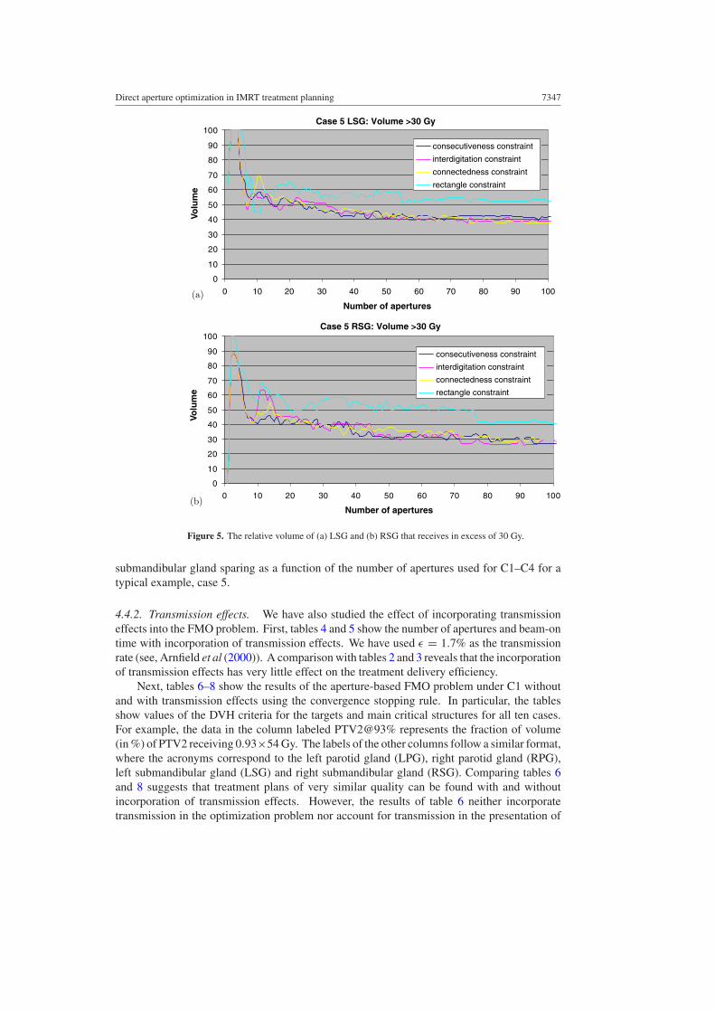
To illustrate how our approach may be used to make a trade-off between treatment planquality and delivery efficiency, figures 4 and 5 show the behavior of target coverage and

Direct aperture optimization in IMRT treatment planning 7347

(a)

Case 5 LSG: Volume >30 Gy

0

10

20

30

40

50

60

70

80

90

100

0 10 20 30 40 50 60 70 80 90 100

Number of apertures

Volu

me

consecutiveness constraint

interdigitation constraint

connectedness constraint

rectangle constraint

(b)

Case 5 RSG: Volume >30 Gy

0

10

20

30

40

50

60

70

80

90

100

0 10 20 30 40 50 60 70 80 90 100

Number of apertures

Volu

me

consecutiveness constraint

interdigitation constraint

connectedness constraint

rectangle constraint

Figure 5. The relative volume of (a) LSG and (b) RSG that receives in excess of 30 Gy.

submandibular gland sparing as a function of the number of apertures used for C1–C4 for atypical example, case 5.

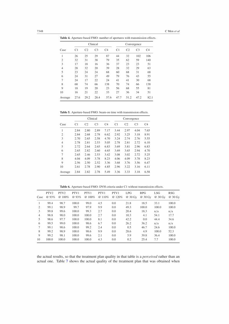
4.4.2. Transmission effects. We have also studied the effect of incorporating transmissioneffects into the FMO problem. First, tables 4 and 5 show the number of apertures and beam-ontime with incorporation of transmission effects. We have used ε = 1.7% as the transmissionrate (see, Arnfield et al (2000)). A comparison with tables 2 and 3 reveals that the incorporationof transmission effects has very little effect on the treatment delivery efficiency.

Next, tables 6–8 show the results of the aperture-based FMO problem under C1 withoutand with transmission effects using the convergence stopping rule. In particular, the tablesshow values of the DVH criteria for the targets and main critical structures for all ten cases.For example, the data in the column labeled PTV2@93% represents the fraction of volume(in %) of PTV2 receiving 0.93×54 Gy. The labels of the other columns follow a similar format,where the acronyms correspond to the left parotid gland (LPG), right parotid gland (RPG),left submandibular gland (LSG) and right submandibular gland (RSG). Comparing tables 6and 8 suggests that treatment plans of very similar quality can be found with and withoutincorporation of transmission effects. However, the results of table 6 neither incorporatetransmission in the optimization problem nor account for transmission in the presentation of

7348 C Men et al

Table 4. Aperture-based FMO: number of apertures with transmission effects.

Clinical Convergence

Case C1 C2 C3 C4 C1 C2 C3 C4

1 26 25 29 87 44 32 102 1062 32 31 38 79 35 62 59 1403 17 18 16 36 37 23 23 514 28 32 20 39 28 32 29 635 23 24 24 68 60 68 31 686 24 31 27 49 79 76 43 557 24 17 22 24 41 41 30 688 68 74 66 138 70 74 66 1389 18 19 20 23 56 68 55 81

10 16 21 22 33 27 36 34 51

Average 27.6 29.2 28.4 57.6 47.7 51.2 47.2 82.1

Table 5. Aperture-based FMO: beam-on time with transmission effects.

Clinical Convergence

Case C1 C2 C3 C4 C1 C2 C3 C4

1 2.84 2.80 2.89 7.17 3.44 2.97 4.04 7.652 2.84 2.68 2.78 6.62 2.92 3.25 3.18 8.913 2.70 2.65 2.58 4.70 3.24 2.74 2.76 5.554 2.78 2.81 2.53 5.05 2.78 2.81 2.72 6.105 2.72 2.64 2.65 6.83 3.69 3.81 2.96 6.836 2.65 2.82 2.60 4.65 3.69 3.65 2.94 4.707 2.65 2.46 2.53 3.42 3.08 3.02 2.72 5.258 4.04 4.09 3.78 8.23 4.06 4.09 3.78 8.239 2.56 2.50 2.52 3.36 3.68 3.76 3.56 6.47

10 2.61 2.78 2.90 4.85 2.96 3.22 3.16 6.11

Average 2.84 2.82 2.78 5.49 3.36 3.33 3.18 6.58

Table 6. Aperture-based FMO: DVH criteria under C1 without transmission effects.

PTV2 PTV2 PTV1 PTV1 PTV1 PTV1 LPG RPG LSG RSGCase @ 93% @ 100% @ 93% @ 100% @ 110% @ 120% @ 30 Gy @ 30 Gy @ 30 Gy @ 30 Gy

1 99.4 98.7 100.0 99.0 4.5 0.0 21.8 18.5 33.1 100.02 99.1 98.9 99.7 97.9 9.9 0.0 49.3 100.0 100.0 100.03 99.8 99.6 100.0 99.3 2.7 0.0 20.4 18.3 n/a n/a4 98.8 98.0 100.0 100.0 2.7 0.0 10.3 4.1 54.1 17.75 98.6 97.7 100.0 100.0 8.1 0.0 42.2 0.0 44.4 34.66 99.5 99.0 100.0 98.6 6.7 0.0 26.2 36.2 n/a n/a7 99.1 98.6 100.0 99.2 2.4 0.0 0.5 46.7 24.6 100.08 99.2 98.9 100.0 98.6 9.9 0.0 28.6 4.9 100.0 52.39 99.2 98.1 100.0 99.6 2.1 0.0 5.9 39.8 36.4 100.0

10 100.0 100.0 100.0 100.0 4.3 0.0 0.2 25.4 7.7 100.0

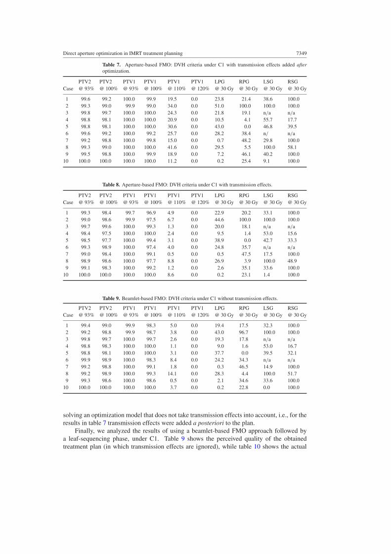
the actual results, so that the treatment plan quality in that table is a perceived rather than anactual one. Table 7 shows the actual quality of the treatment plan that was obtained when

Direct aperture optimization in IMRT treatment planning 7349

Table 7. Aperture-based FMO: DVH criteria under C1 with transmission effects added afteroptimization.

PTV2 PTV2 PTV1 PTV1 PTV1 PTV1 LPG RPG LSG RSGCase @ 93% @ 100% @ 93% @ 100% @ 110% @ 120% @ 30 Gy @ 30 Gy @ 30 Gy @ 30 Gy

1 99.6 99.2 100.0 99.9 19.5 0.0 23.8 21.4 38.6 100.02 99.3 99.0 99.9 99.0 34.0 0.0 51.0 100.0 100.0 100.03 99.8 99.7 100.0 100.0 24.3 0.0 21.8 19.1 n/a n/a4 98.8 98.1 100.0 100.0 20.9 0.0 10.5 4.1 55.7 17.75 98.8 98.1 100.0 100.0 30.6 0.0 43.0 0.0 46.8 39.56 99.6 99.2 100.0 99.2 25.7 0.0 28.2 38.4 n/ n/a7 99.2 98.8 100.0 99.8 15.0 0.0 0.7 48.2 29.8 100.08 99.3 99.0 100.0 100.0 41.6 0.0 29.5 5.5 100.0 58.19 99.5 98.8 100.0 99.9 18.9 0.0 7.2 46.1 40.2 100.0

10 100.0 100.0 100.0 100.0 11.2 0.0 0.2 25.4 9.1 100.0

Table 8. Aperture-based FMO: DVH criteria under C1 with transmission effects.

PTV2 PTV2 PTV1 PTV1 PTV1 PTV1 LPG RPG LSG RSGCase @ 93% @ 100% @ 93% @ 100% @ 110% @ 120% @ 30 Gy @ 30 Gy @ 30 Gy @ 30 Gy

1 99.3 98.4 99.7 96.9 4.9 0.0 22.9 20.2 33.1 100.02 99.0 98.6 99.9 97.5 6.7 0.0 44.6 100.0 100.0 100.03 99.7 99.6 100.0 99.3 1.3 0.0 20.0 18.1 n/a n/a4 98.4 97.5 100.0 100.0 2.4 0.0 9.5 1.4 53.0 15.65 98.5 97.7 100.0 99.4 3.1 0.0 38.9 0.0 42.7 33.36 99.3 98.9 100.0 97.4 4.0 0.0 24.8 35.7 n/a n/a7 99.0 98.4 100.0 99.1 0.5 0.0 0.5 47.5 17.5 100.08 98.9 98.6 100.0 97.7 8.8 0.0 26.9 3.9 100.0 48.99 99.1 98.3 100.0 99.2 1.2 0.0 2.6 35.1 33.6 100.0

10 100.0 100.0 100.0 100.0 8.6 0.0 0.2 23.1 1.4 100.0

Table 9. Beamlet-based FMO: DVH criteria under C1 without transmission effects.

PTV2 PTV2 PTV1 PTV1 PTV1 PTV1 LPG RPG LSG RSGCase @ 93% @ 100% @ 93% @ 100% @ 110% @ 120% @ 30 Gy @ 30 Gy @ 30 Gy @ 30 Gy

1 99.4 99.0 99.9 98.3 5.0 0.0 19.4 17.5 32.3 100.02 99.2 98.8 99.9 98.7 3.8 0.0 43.0 96.7 100.0 100.03 99.8 99.7 100.0 99.7 2.6 0.0 19.3 17.8 n/a n/a4 98.8 98.3 100.0 100.0 1.1 0.0 9.0 1.6 53.0 16.75 98.8 98.1 100.0 100.0 3.1 0.0 37.7 0.0 39.5 32.16 99.9 98.9 100.0 98.3 8.4 0.0 24.2 34.3 n/a n/a7 99.2 98.8 100.0 99.1 1.8 0.0 0.3 46.5 14.9 100.08 99.2 98.9 100.0 99.3 14.1 0.0 28.3 4.4 100.0 51.79 99.3 98.6 100.0 98.6 0.5 0.0 2.1 34.6 33.6 100.0

10 100.0 100.0 100.0 100.0 3.7 0.0 0.2 22.8 0.0 100.0

solving an optimization model that does not take transmission effects into account, i.e., for theresults in table 7 transmission effects were added a posteriori to the plan.

Finally, we analyzed the results of using a beamlet-based FMO approach followed bya leaf-sequencing phase, under C1. Table 9 shows the perceived quality of the obtainedtreatment plan (in which transmission effects are ignored), while table 10 shows the actual

7350 C Men et al

Table 10. Beamlet-based FMO: DVH criteria under C1 with transmission effects.

PTV2 PTV2 PTV1 PTV1 PTV1 PTV1 LPG RPG LSG RSGCase @ 93% @ 100% @ 93% @ 100% @ 110% @ 120% @ 30 Gy @ 30 Gy @ 30 Gy @ 30 Gy

1 99.9 99.8 100.0 100.0 69.1 1.3 32.5 27.2 55.1 100.02 99.6 99.5 100.0 99.9 96.5 0.4 59.1 99.3 100.0 100.03 99.9 99.9 100.0 100.0 94.3 0.1 25.8 21.0 n/a n/a4 99.7 99.5 100.0 100.0 100.0 6.8 17.7 10.4 74.6 40.35 99.6 99.3 100.0 100.0 83.1 1.3 48.0 2.1 56.5 56.86 99.9 99.4 100.0 100.0 75.8 0.0 33.6 41.7 n/a n/a7 99.7 99.5 100.0 100.0 96.7 1.8 4.4 59.3 42.1 100.08 99.7 99.5 100.0 100.0 86.9 1.4 40.2 18.5 100.0 70.699 99.8 99.7 100.0 100.0 72.7 0.0 9.4 54.5 51.4 100.0

10 100.0 100.0 100.0 100.0 100.0 70.6 4.7 41.7 16.1 100.0

quality of the treatment plan (in which transmission effects are added to the final treatmentplan).

From the latter two tables, it is clear that using a beamlet-based FMO optimizationapproach may severely underestimate target hotspots (overdosing) and effects on criticalstructures. The direct aperture optimization approach with transmission effects incorporated,however, provides a high-quality treatment plan with, on average, a comparable number ofapertures and beam-on time. Taking case 5 as an example, a treatment plan that ignoredtransmission effects appeared to spare all four saliva glands, while less than 10% of PTV1received in excess of 110% of its the prescription dose. Adding transmission effects to theplan found using beamlet-based FMO showed that in fact only two saliva glands were sparedwith the PTV1 hotspot increasing to over 80%. Incorporating transmission effects into theaperture-based FMO model showed that it was possible to spare all saliva glands and that keepthe dose to PTV1 in excess of 110% of its prescribed dose to about 3%.

5. Concluding remarks and future research

In this paper, we used a direct aperture optimization approach to design radiation therapytreatment plans for individual patients. This approach allows us to make a sound trade-off between treatment plan quality and delivery efficiency. In addition, our model is ableto explicitly incorporate transmission effects, which can dramatically affect the quality of atreatment plan but are ignored by the most existing FMO models. Future research could extendthe research in this paper by explicitly incorporating a measure of treatment plan efficiency,such as beam-on time, into the optimization model.

References

Ahuja R K and Hamacher H W 2005 A network flow algorithm to minimize beam-on time for unconstrained multileafcollimator problems in cancer radiation therapy Networks 45 36–41

Aleman D M, Glaser D, Romeijn H E and Dempsey J F 2007 A primal-dual interior point algorithm for fluencemap optimization in intensity modulated radiation therapy treatment planning Technical Report (Gainesville,Florida: Department of Industrial and Systems Engineering, University of Florida)

Arnfield M R, Siebers J V, Kim J O, Wu Q, Keall P J and Mohan R 2000 A method for determining multileafcollimator transmission and scatter for dynamic intensity modulated radiotherapy Med. Phys. 27 2231–41

Baatar D, Hamacher H W, Ehrgott M and Woeginger G J 2005 Decomposition of integer matrices and multileafcollimator sequencing Discrete Appl. Math. 152 6–34

Bates J and Constable R 1985 Proofs as programs ACM Trans. Program. Lang. Syst. 7 113–36

Direct aperture optimization in IMRT treatment planning 7351

Bazaraa M S, Sherali H D and Shetty C M 2006 Nonlinear Programming: Theory and Algorithms 3rd edn (NewYork: Wiley)

Bednarz G, Michalski D, Houser C, Huq M S, Xiao Y, Anne P R and Galvin J M 2002 The use of mixed-integerprogramming for inverse treatment planning with pre-defined field segments Phys. Med. Biol. 47 2235–45

Bentley J 1986 Programming Pearls (Reading, MA: Addison-Wesley)Boland N, Hamacher H W and Lenzen F 2004 Minimizing beam-on time in cancer radiation treatment using multileaf

collimators Networks 43 226–40Bortfeld T R, Kahler D L, Waldron T J and Boyer A L 1994 X-ray field compensation with multileaf collimators Int.

J. Radiat. Oncol. Biol. Phys. 28 723–370Dai J and Hu Y 1999 Intensity-modulation radiotherapy using independent collimators: an algorithm study Med.

Phys. 26 2562–70Dai J and Zhu Y 2001 Minimizing the number of segments in a delivery sequence for intensity-modulated radiation

therapy with a multileaf collimator Med. Phys. 28 2113–20Earl M A, Afghan M K N, Yu C X, Jiang Z and Shepard D M 2007 Jaws-only IMRT using direct aperture optimization

Med. Phys. 34 307–14Engel K 2005 A new algorithm for optimal multileaf collimator field segmentation Discrete Appl. Math.

152 35–51Hamacher H W and Kufer K 2002 Inverse radiation therapy planning—a multiple objective optimization approach

Discrete Appl. Math. 118 145–61Kalinowski T 2004 The algorithmic complexity of the minimization of the number of segments in multileaf collimator

field segmentation Technical Report (Rostock, Germany: Fachbereich Mathematik, Universitat Rostock)Kalinowski T 2005a A duality based algorithm for multileaf collimator field segmentation with interleaf collision

constraint Discrete Appl. Math. 152 52–88Kalinowski T 2005b Reducing the number of monitor units in multileaf collimator field segmentation Phys. Med.

Biol. 50 1147–61Kamath S, Sahni S, Li J, Palta J and Ranka S 2003 Leaf sequencing algorithms for segmented multileaf collimation

Phys. Med. Biol. 48 307–24Kamath S, Sahni S, Palta J and Ranka S 2004a Algorithms for optimal sequencing of dynamic multileaf collimators

Phys. Med. Biol. 49 33–54Kamath S, Sahni S, Palta J, Ranka S and Li J 2004b Optimal leaf sequencing with elimination of tongue-and-groove

underdosage Phys. Med. Biol. 49 N7–N19Kamath S, Sahni S, Ranka S, Li J and Palta J 2004c A comparison of step-and-shoot leaf sequencing algorithms that

eliminate tongue-and-groove effects Phys. Med. Biol. 49 3137–43Kamath S, Sahni S, Ranka S, Li J and Palta J 2004d Optimal field splitting for large intensity-modulated fields Med.

Phys. 31 3314–23Kim Y, Verhey L J and Xia P 2007 A feasibility study of using conventional jaws to deliver IMRT plans in the

treatment of prostate cancer Phys. Med. Biol. 52 2147–56Kufer K, Monz M, Scherrer A, Trinkaus H L, Bortfeld T and Thieke C 2003 Intensity Modulated Radiotherapy—a

large scale multi-criteria programming problem OR Spektrum 25 223–49Kutcher G J and Burman C 1989 Calculation of complication probability factors for non-uniform normal tissue

irradiation: the effective volume method Int. J. Radiat. Oncol. Biol. Phys. 16 1623–30Langer M, Thai V and Papiez L 2001 Improved leaf sequencing reduces segments or monitor units needed to deliver

IMRT using multileaf collimators Med. Phys. 28 2450–8Lee E K, Fox T and Crocker I 2000 Optimization of radiosurgery treatment planning via mixed integer programming

Med. Phys. 27 995–1004Lee E K, Fox T and Crocker I 2003 Integer programming applied to intensity-modulated radiation treatment planning

Ann. Oper. Res. 119 165–81Lenzen F 2000 An integer programming approach to the multileaf collimator problem Master’s Thesis Department

of Mathematics, University of Kaiserslautern, Kaiserslautern, GermanyLim G J and Choi J 2006 A two-stage integer programming approach for optimizing leaf sequence in IMRT Technical

Report (Houston, Texas: Department of Industrial Engineering, University of Houston)Lu X and Chin L 1993 Sampling techniques for the evaluation of treatment plans Med. Phys. 20 151–61Niemierko A 1997 Reporting and analyzing dose distributions: a concept of equivalent uniform dose Med. Phys.

24 103–10Niemierko A 1999 A generalized concept of equivalent uniform dose Med. Phys. 26 1100Preciado-Walters F, Rardin R, Langer M and Thai V 2004 A coupled column generation, mixed integer approach to

optimal planning of intensity modulated radiation therapy for cancer Math. Program. 101 319–38Que W 1999 Comparison of algorithms for multileaf collimator field segmentation Med. Phys. 26 2390–6

7352 C Men et al

Radiation Therapy 0000 Oncology Group 2000 H-0022: A phase I/II study of conformal and intensity modulatedirradiation for oropharyngeal cancer http://www.rtog.org/members/protocols/h0022/h0022.pdf

Radiation Therapy 0000 Oncology Group 2002 H-0225: A phase II study of intensity modulated radiation therapy(IMRT) +/− chemotherapy for nasopharyngeal cancer http://www.rtog.org/members/protocols/0225/ 0225.pdf

Rockafellar R T and Uryasev S 2000 Optimization of conditional value-at-risk J. Risk 2 21–41Romeijn H E, Ahuja R K, Dempsey J F and Kumar A 2005 A column generation approach to radiation therapy

treatment planning using aperture modulation SIAM J. Optim. 15 838–62Romeijn H E, Ahuja R K, Dempsey J F and Kumar A 2006 A new linear programming approach to radiation therapy

treatment planning problems Oper. Res. 54 201–16Romeijn H E, Ahuja R K, Dempsey J F, Kumar A and Li J G 2003 A novel linear programming approach to fluence

map optimization for intensity modulated radiation therapy treatment planning Phys. Med. Biol. 48 3521–42Romeijn H E, Dempsey J F and Li J G 2004 A unifying framework for multi-criteria fluence map optimization models

Phys. Med. Biol. 49 1991–2013Shepard D M, Earl M A, Li X A, Naqvi S and Yu C 2002 Direct aperture optimization: a turnkey solution for

step-and-shoot IMRT Med. Phys. 29 1007–18Shepard D M, Ferris M C, Olivera G H and Mackie T R 1999 Optimizing the delivery of radiation therapy to cancer

patients SIAM Rev. 41 721–44Siebers J V, Lauterbach M, Keall P J and Mohan R 2002 Incorporating multi-leaf collimator leaf sequencing into

iterative IMRT optimization Med. Phys. 29 952–9Siochi R A C 1999 Minimizing static intensity modulation delivery time using an intensity solid paradigm Int. J.

Radiat. Oncol. Biol. Phys. 43 671–89Taskın Z C, Smith J C, Romeijn H E and Dempsey J F 2007 Optimal multileaf collimator leaf sequencing in IMRT

treatment planning Technical Report (Gainesville, Florida: Department of Industrial and Systems Engineering,University of Florida)

Tsien C, Eisbruch A, McShan D, Kessler M, Marsh R and Fraass B 2003 Intensity-modulated radiation therapy (IMRT)for locally advanced paranasal sinus tumors: incorporating clinical decisions in the optimization process Int. J.Radiat. Oncol. Biol. Phys. 55 776–84

Xia P and Verhey L J 1998 Multileaf collimator leaf sequencing algorithm for intensity modulated beams with multiplestatic segments Med. Phys. 25 1424–34