Direct and inverse discrete Zernike transform · PDF file2Departmento de Física Aplicada, ... free-space communications, etc. The modal representation of a function (wavefront,

Direct and inverse discrete Zernike transform

Rafael Navarro,1,*

Justo Arines,2

and Ricardo Rivera1

1ICMA, Universidad de Zaragoza and Consejo Superior de Investigaciones Científicas, Facultad de Ciencias, Pedro Cerbuna 12, 50009 Zaragoza, Spain

2Departmento de Física Aplicada, Facultad de Ciencias, Pedro Cerbuna 12, 50009 Zaragoza, Spain *[email protected]

Abstract: An invertible discrete Zernike transform, DZT is proposed and implemented. Three types of non-redundant samplings, random, hybrid (perturbed deterministic) and deterministic (spiral) are shown to provide completeness of the resulting sampled Zernike polynomial expansion. When completeness is guaranteed, then we can obtain an orthonormal basis, and hence the inversion only requires transposition of the matrix formed by the basis vectors (modes). The discrete Zernike modes are given for different sampling patterns and number of samples. The DZT has been implemented showing better performance, numerical stability and robustness than the standard Zernike expansion in numerical simulations. Non-redundant (critical) sampling along with an invertible transformation can be useful in a wide variety of applications.

©2009 Optical Society of America

OCIS codes: (080.1005) Aberration expansions; (010.7350) Wave-front sensing; (110.7348) Wavefront encoding ; (220.1010) Aberrations (global).

References and links

1. V. N. Mahajan, “Zernike polynomials and wavefront fitting,” in Optical Shop Testing, 3rd ed., D. Malacara, ed. (Wiley, New York, 2007).

2. R. Navarro, and E. Moreno-Barriuso, “Laser ray-tracing method for optical testing,” Opt. Lett. 24(14), 951–953 (1999).

3. R. J. Noll, “Phase estimates from slope–type wave–front sensors,” J. Opt. Soc. Am. 68(1), 139–140 (1978). 4. R. Cubalchini, “Modal wave-front estimation from phase derivative measurements,” J. Opt. Soc. Am. 69(7),

972–977 (1979). 5. J. Y. Wang, and D. E. Silva, “Wave-front interpretation with Zernike polynomials,” Appl. Opt. 19(9), 1510–1518

(1980). 6. R. K. Tyson, Principles of Adaptive Optics (Academic, Boston, 1991). 7. J. Alda, and G. D. Boreman, “Zernike-based matrix model of deformable mirrors: optimization of aperture size,”

Appl. Opt. 32, 2431–2438 (1993). 8. G. D. Love, “Wave-front correction and production of Zernike modes with a liquid-crystal spatial light

modulator,” Appl. Opt. 36(7), 1517–1520 (1997). 9. C.-J. Kim, “Polynomial fit of interferograms,” Appl. Opt. 21(24), 4521–4525 (1982). 10. H. van Brug, “Zernike polynomials as a basis for wave-front fitting in lateral shearing interferometry,” Appl.

Opt. 36(13), 2788–2790 (1997). 11. B. Qi, H. Chen, and N. Dong, “Wavefront fitting of interferograms with Zernike polynomials,” Opt. Eng. 41(7),

1565–1569 (2002). 12. J. Nam, and J. Rubinstein, “Numerical reconstruction of optical surfaces,” J. Opt. Soc. Am. A 25(7), 1697–1709

(2008). 13. J. Schwiegerling, J. Greivenkamp, and J. Miller, “Representation of videokeratoscopic height data with Zernike

polynomials,” J. Opt. Soc. Am. A 12(10), 2105–2113 (1995). 14. R. J. Noll, “Zernike polynomials and atmospheric turbulence,” J. Opt. Soc. Am. 66(3), 207–211 (1976). 15. J. Herrmann, “Cross coupling and aliasing in modal wave-front estimation,” J. Opt. Soc. Am. 71(8), 989–992

(1981). 16. J. Herrmann, “Least-squares wave front errors of minimum norm,” J. Opt. Soc. Am. 70(1), 28–35 (1980). 17. O. Soloviev, and G. Vdovin, “Hartmann-Shack test with random masks for modal wavefront reconstruction,”

Opt. Express 13(23), 9570–9584 (2005). 18. M. Ares, and S. Royo, “Comparison of cubic B-spline and Zernike-fitting techniques in complex wavefront

reconstruction,” Appl. Opt. 45(27), 6954–6964 (2006). 19. L. Diaz-Santana, G. Walker, and S. X. Bará, “Sampling geometries for ocular aberrometry: A model for

evaluation of performance,” Opt. Express 13(22), 8801–8818 (2005).

#114072 - $15.00 USD Received 9 Jul 2009; revised 20 Nov 2009; accepted 4 Dec 2009; published 18 Dec 2009

(C) 2009 OSA 21 December 2009 / Vol. 17, No. 26 / OPTICS EXPRESS 24269

20. W. H. Southwell, “Wave–front estimation from wave–front slope measurements,” J. Opt. Soc. Am. 70(8), 998–1006 (1980).

21. E. E. Silbaugh, B. M. Welsh, and M. C. Roggemann, “Characterization of Atmospheric Turbulence Phase Statics Using Wave-Front Slope Measurements,” J. Opt. Soc. Am. A 13(12), 2453–2460 (1996).

22. J. Liang, B. Grimm, S. Goelz, and J. F. Bille, “Objective measurement of wave aberrations of the human eye with use of a Hartmann-Shack wave-front sensor,” J. Opt. Soc. Am. A 11, 1949–1957 (1994).

23. E. Anderson, Z. Bai, C. Bischof, S. Blackford, J. Demmel, J. Dongarra, J. Du Croz, A. Greenbaum, S. Hammarling, A. McKenney, and D. Sorensen, LAPACK User's Guide, 3rd Ed., (SIAM, Philadelphia, 1999), http://www.netlib.org/lapack/lug/lapack_lug.html.

24. N. U. Mayall, and S. Vasilevskis, “Quantitative tests of the Lick Observatory 120-Inch mirror,” Astron. J. 65, 304–317 (1960).

25. R. Navarro, “Objective refraction from aberrometry: theory,” J. Biomed. Opt. 14(2), 024021 (2009). 26. D. Malacara-Hernandez, “Wavefront fitting with discrete orthogonal polynomials in a unit radius circle,” Opt.

Eng. 29(6), 672–675 (1990). 27. D. J. Fischer, J. T. O'Bryan, R. Lopez, and H. P. Stahl, “Vector formulation for interferogram surface fitting,”

Appl. Opt. 32(25), 4738–4743 (1993). 28. J. Arines, E. Pailos, P. Prado, and S. Bará, “The contribution of the fixational eye movements to the variability of

the measured ocular aberration,” Ophthalmic Physiol. Opt. 29(3), 281–287 (2009).

1. Introduction

The Zernike polynomial (ZP) expansion is extremely useful in optics because ZPs form a complete orthogonal basis on a circle of unit radius. Since many optical instruments have a circular symmetry and circular pupil, ZP expansion can be used to describe any function at the pupil plane; in particular optical path differences (OPD), wavefront phase or wave aberration. Therefore, applications include computing and optimization (optical design) [1], optical testing [2], wavefront sensing [3–5], adaptive optics [6,7], wavefront shaping [8], interferometry [9–11], surface metrology (profilometry, topography) [12,13] or atmospheric optics [14] among others. The modal description provided by ZPs has been highly successful in all these fields of application. Nowadays Zernike polynomials are present in current technologies in ophthalmology, ground-based telescopes, free-space communications, etc.

The modal representation of a function (wavefront, OPD, surface, etc.) over a circular pupil in terms of ZPs is:

( ) ( ),

, ,m m

n n

n m

W c Zρ θ ρ θ=∑ (1)

where m

nc are the expansion coefficients; θρ, are polar coordinates with origin at the pupil

centre. Here pupRR=ρ is a normalized radius, since the ZPs are orthogonal only within a

circle of unit radius. ZPs are separable into radial and angular parts, and include a normalization factor N to guarantee orthonormality:

( )( )( )

cos for 0,

sin for 0

mm

n nm

n mm

n n

N R m mZ

N R m m

ρ θρ θ

ρ θ

≥ =

− < (2)

where the radial part is given by

( )( ) 2

2

0

( 1) ( )!,

! 0.5( ) ! 0.5( ) !

n m sm n s

n

s

n sR

s n m s n m sρ ρ

−−

=

− −=

+ − − − ∑ (3)

the normalization coefficient is

0

2( 1)

1

m

n

m

nN

δ+

=+

(4)

and δm0 is the Kronecker delta function. The radial order n is integer positive, and the angular frequency m can only take on values -n, -n + 2, -n + 4, ... n.



Despite the importance of the basis of Zernike polynomials, they present several drawbacks in practical applications. This is a reason why different authors prefer to use other alternative basis functions (Fourier, splines, etc). A major problem is that in real applications one works with discrete (sampled) arrays of data rather than with continuous functions, and then Zernike polynomials do not form a complete basis on the sampled circle [5]. As an example, the RMS error is probably the most common metric used to determine the difference between two wavefronts or between a wavefront and some ideal reference. By orthonormality

of ZPs, one can compute that RMS error either point by point (iw ) or between coefficients

(m

nc ) of the Zernike expansion. However, with a discrete number of samples, one finds that

these two metrics provide different results in general:

2 2

,

.m

i n

i n m

w I c≠∑ ∑ (5)

This is because sampled ZPs are neither complete nor orthogonal, and as a result the discrete expansion is not invertible.

In the discrete case, Eq. (1) can be written as W = ZC, where Z is a matrix whose columns are sampled Zernike polynomials and W and C are column vectors corresponding to samples

and coefficients of the wavefront respectively. The lack of completeness implies that Z−−−−1

does not exist and hence we cannot solve Eq. (1) to obtain the coefficients. The standard way to overcome this problem is to oversample the wavefront and estimate a number of coefficients J lower than the number of samples I (J < I). The coefficients are then estimated by least squares fit to the data. In matrix notation, this is equivalent to compute the Moore-Penrose pseudoinverse of Z. (Z is not square as it has more rows –samples- than columns –coefficients-):

( ) 1

.T T

−=C Z Z Z W⌢

(6)

The tilde means estimated, since the wavefront expansion is approximated. This estimation is optimal under a least squares criterion (minimum RMS error), but may not be exact (due to mode coupling and aliasing [15–17]) and always requires a redundant sampling. Therefore, the estimation of the coefficients of the Zernike expansion is still an open problem, which has attracted the interest of many researchers.

Different studies have focused on alternative basis functions (Fourier, splines, etc [18].), estimation methods, or sampling patterns (random, optimized designs, etc [17,19].). In addition to these general problems, wavefront sensing (estimation from slope measurements [20]) is especially interesting in many applications: atmospheric turbulence measurements [21], optical testing [2], adaptive optics [6], ophthalmology [22], etc. In wavefront sensing, the coefficients are estimated from wavefront partial derivatives (ignoring constant factors):

( ) 1T

−= Z Z ZC D D D M⌢

(7)

where vector M contains the measurements (displacements along X and along Y of spots at the image of the sensor, which are proportional to wavefront slopes) and DZ is the matrix formed by the partial derivatives of the ZPs with respect to X and Y. Then, we have a matrix form similar to Eq. (6), but with the additional problem that the derivatives of ZPs do not form a basis even for continuous signals. This is somehow compensated by the fact that the dimensions of M (and columns of DZ) are 2I (double number of samples).

In summary, the estimation of the coefficients of the Zernike expansion relies on redundancy (oversampling). Leaving wavefront sensing (Eq. (7) apart, and focusing on the more basic problem of inverting Eq. (1), to compute the coefficients of the Zernike expansion, our goal is to find an invertible discrete transform. When invertible, the discrete transform can be expressed as a square matrix (I = J), and that matrix must have an inverse. Furthermore, if



the basis vectors (matrix columns) are orthonormal, then the inverse transform (matrix) is equal to its transpose, which ensures numerical stability. For this purpose, we will depart from the Zernike polynomial basis on a continuous circle, and study the problem of completeness in the discrete case; in particular, the role of the sampling pattern. Then we find that determined types of non redundant sampling patterns do ensure completeness. Here we introduce the spiral pattern and compare it with random sampling grids. Once the problem of completeness is overcome, then it is straightforward to apply the Gram-Schmidt method to obtain an orthonormal basis over the sampled circular pupil. Then, we compute the discrete Zernike modes for different sampling patterns and number of samples. Finally, we implement the direct and inverse DZT (discrete Zernike transform) and evaluate its performance with some examples.

2. Discrete Zernike transform

For continuous signals, since ZPs form a complete orthonormal basis, we can solve Eq. (1) for the coefficients. Orthonormality implies that we can compute the coefficients as the projections (inner product) of the function W on each basis function:

( ) ( )1 2

0 0

, , .m m

n nc W Z d d

π

ρ θ ρ θ ρ θ ρ= ∫ ∫ (8)

In what follows, we study how to construct an orthonormal basis functions for the discrete case, so that we can apply a similar recipe to compute the coefficients, i.e. by simple transposition of the elements of the basis.

In real applications, we will have a discrete (sampled) function j j

i i

j

W c Z=∑ ( ZCW = in

matrix notation), where we merged indexes n, m into a single index ( )( ) 22 mnnj ++=

(starting with j = 0). For a given maximum order N of the polynomials, the total number of modes will be ( ) 231 ++= NNJ . Let us investigate if there exist conditions where we can

invert matrix Z and solve for WZC1−= . A necessary condition is Z to be square, so that the

number of coefficients equals the number of samples J = I. In what follows we will refer to this case as critical sampling.

There are two common metrics to check whether a matrix can be inverted. The necessary condition is the rank ( ) JIRank ==Z . This guarantees that the matrix is not singular, and this

is in fact the condition for completeness. In principle, this is a sufficient condition, but a further requirement is related to the real accuracy and numerical stability of the matrix inversion. A commonly used metric for numerical stability is the 2-norm condition number of the matrix; i.e. the ratio of the largest singular value of Z to the smallest [23]. When the condition number is near 1, the matrix is well-conditioned. In what follows we have used the inverse of the condition number which is always between 0 and 1.

We have computed both the rank and condition number of matrix Z for different sampling patterns and number of samples. Some of these sampling patterns are depicted in Fig. 1. Square and hexagonal patterns are typical in Hartmann-Shack wavefront sensors, whereas hexapolar patterns are often used in optical design. All these sampling patterns yield singular

Z matrices ( ( ) IRank <Z and ( ) 0=ZDet ) as shown in Table 1. Perhaps, these types of

regular patterns are not appropriate to sample Zernike polynomials. In polar coordinates these schemes are not so regular and highly redundant (both in ρ and θ).

Different studies [15–17,19] have shown a strong influence of the sampling pattern on wavefront reconstruction from wavefront slopes. In particular, random patterns show better performance [17,19]. Perhaps, the subjacent effect has to do with the fact that random patterns are non redundant in ρ and θ (i.e. the values of coordinates are never repeated) which may help to avoid Z to be singular. Since all Zernike polynomials are different from 0, singularity of Z must come from redundancy between sampled basis functions. Then, let us suppose that



such redundancy in the Z matrix has to do with redundancy (repetition) of values of coordinates at the sampling points, and verify this idea through numerical simulation.

For this purpose, we have implemented three cases with (i) pure random sampling; (ii) small random perturbations of regular sampling grids; and (iii) non-redundant deterministic sampling.

2.1. Random and deterministic sampling patterns

Random patterns (i) were generated as follows. Each sampling point is obtained by adding a random displacement to the coordinates of the previous sampling element. These displacements have a Gaussian distribution with zero mean and standard deviation equal to the diameter of the sampling element. Non-overlapping between samples and total inclusion of the sampling element into the measured pupil were imposed. Several masks were generated and compared in terms of the condition number of the Z matrix obtained for each of them, in order to choose the best realization.

The perturbed regular sampling patterns (ii) were implemented by adding small random Cartesian displacements (

yx εε , ) to the sampling points of regular grids. These perturbations

have a Gaussian distribution with zero mean, and their magnitude is determined by the

standard deviation σ. We have performed simulations with perturbations ranging from 10−8

to

10−2

in pupil radius units. Finally, we designed regular (deterministic) non redundant sampling patterns (iii). Regular

sampling patterns are commonly obtained by convolution of the function to be sampled with a

Dirac comb. Let us start with the angular coordinate. To sample the interval [0, maxθ ] with I

equispaced samples, the interval will be ( )1max −= Iθδθ . We could apply a similar sampling

to ρ. If the comb is 2D (2-dimensional) we obtain a pure polar sampling, which is redundant in both coordinates. A way to avoid redundancy is to apply 1D Dirac combs to both

coordinates; or in other words to make ρ proportional to θ and set CNπθ 2max = . In this way

we obtain a rolled 1D pattern, which is a spiral with NC cycles covering a circular area with

radiusmaxmax θρ ∝ . To completely avoid redundancy, we have to be careful with the

periodicity of the angular variable, i.e. we need to guarantee that the number of samples per cycle δθπ2=NSPC is non integer. The difference between polar and spiral patterns is that

the former is a purely 2-dimensional whereas the spiral is obtained by rolling a 1D pattern. Despite their different nature both can adequately cover a circular domain. The linear spiral, however, has the problem that the density of samples per unit of area is high at the center and decreases towards the edge. One way to avoid that problem is to use an array of spirals to form an helical pattern [24]. Here, however, the goal was to avoid redundancy, and we implemented a sampling scheme based on a single Fermat or parabolic spiral, where the radial

coordinate is proportional to the square root of θ ( ( ) maxθθθρ = ) to ensure that 1≤ρ . With

the parabolic spiral we can keep the density of samples nearly constant when the angle is sampled uniformly. In a first approximation, this occurs when the number of cycles is

proportional to the square root of the number of samples πINc ≈ . Usually Nc is chosen to

be integer, but in some cases this could result in a redundant sampling. If that happens (see

below) we add 1/2 cycle to break periodicity: Thus, we have two cases ( )πINc int= or

( ) 5.0int += πINc; where “int” means nearest integer. In terms of the number of cycles

( )12 −= INcπδθ . By definition, the radial coordinate ρ is never repeated, and with the

additional condition that the sampling is not periodic in π2 (i.e. the number of samples per

cycle is not integer, ( ) iNINSPC c ≠−== 12 δθπ ), then we avoid any redundancy in both

radial and angular coordinates. The two examples implemented here correspond to orders N = 7 and N = 12 and represent the two possible cases of Nc. In the first case we have J = I = 36;



then Nc = 3, 5386.0=δθ radians and NSPC = 11.667. Since this is not an integer number,

the sampling is non redundant. In the second example, N = 12 and I = J = 91. If we choose an

integer value Nc = 5, 349.0=δθ but then we will have NSPC = 18 and the sampling would be

periodic in θ; i.e. redundant. We can avoid that redundancy by adding 0.5 cycles so that

Nc = 5.5, then 384.0=δθ radians and NSPC = 16.36.

In some applications [25] it may be convenient to avoid the origin, starting the spiral with

an initial sample at kδθθ =1 with k >>1 (in particular for k = ∞ the initial point will be at the

origin). Finally, the last sample of the spiral has to strictly meet the condition ρΙ < 1 to avoid partial occlusion of the marginal samples by the pupil. One possible criterion is to keep the area covered by this last sample equal to the average. As an approximation, here we impose the radial distance of the last sample to the pupil edge to be equal to half the width of the last

cycle: ( )NSPCIII −−=− ρρρ 211 ; solving for NSPCII −+= ρρ 3132 ; and in terms of

Nc: ( ) ccI NN 13132 −+=ρ . (In the examples 36=Iρ = 0.9388 for I = 36 and

91=Iρ = 0.9682 respectively.) Now, the sampling grid is fully determined by

( )δθδθθ 1−+= iki with i = 1, 2,...I and

IiIi θθρρ = . Therefore, given a maximum

order N of Zernike polynomials, we want as many samples as Zernike modes,

( ) 231 ++== NNJI ; then assign a number of cycles (first option Nc integer when NSPC is

non integer; or add 0.5 to avoid periodicity if NSPC integer). Finally choose a value for k to have the spiral sampling completely determined.

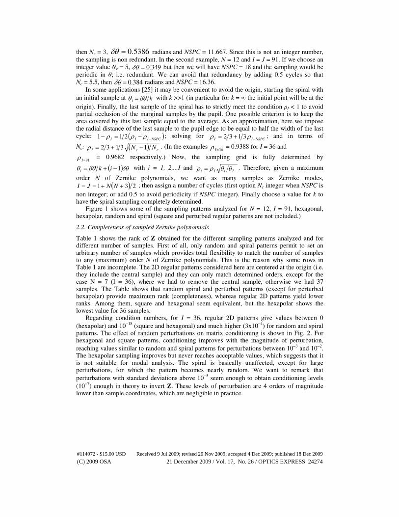
Figure 1 shows some of the sampling patterns analyzed for N = 12, I = 91, hexagonal, hexapolar, random and spiral (square and perturbed regular patterns are not included.)

2.2. Completeness of sampled Zernike polynomials

Table 1 shows the rank of Z obtained for the different sampling patterns analyzed and for different number of samples. First of all, only random and spiral patterns permit to set an arbitrary number of samples which provides total flexibility to match the number of samples to any (maximum) order N of Zernike polynomials. This is the reason why some rows in Table 1 are incomplete. The 2D regular patterns considered here are centered at the origin (i.e. they include the central sample) and they can only match determined orders, except for the case N = 7 (I = 36), where we had to remove the central sample, otherwise we had 37 samples. The Table shows that random spiral and perturbed patterns (except for perturbed hexapolar) provide maximum rank (completeness), whereas regular 2D patterns yield lower ranks. Among them, square and hexagonal seem equivalent, but the hexapolar shows the lowest value for 36 samples.

Regarding condition numbers, for I = 36, regular 2D patterns give values between 0

(hexapolar) and 10−18

(square and hexagonal) and much higher (3x10−4

) for random and spiral patterns. The effect of random perturbations on matrix conditioning is shown in Fig. 2. For hexagonal and square patterns, conditioning improves with the magnitude of perturbation,

reaching values similar to random and spiral patterns for perturbations between 10−3

and 10−2

. The hexapolar sampling improves but never reaches acceptable values, which suggests that it is not suitable for modal analysis. The spiral is basically unaffected, except for large perturbations, for which the pattern becomes nearly random. We want to remark that

perturbations with standard deviations above 10−5

seem enough to obtain conditioning levels

(10−7

) enough in theory to invert Z. These levels of perturbation are 4 orders of magnitude lower than sample coordinates, which are negligible in practice.



R91 S91

H91 HP91

Fig. 1. Examples of sampling patterns with 91 points providing singular (hexagonal and hexapolar, upper panels) and invertible (random and spiral, lower panels) (Z).

Condition numbers of the order of 10−4

obtained for random and spiral patterns for I = 36

permit us to compute Z−−−−1

with a reasonable accuracy. However, as the number of samples increases, the conditioning gets worse. For example, in the case of I = 91 samples, spiral and

random patterns yield condition numbers of the order of 10−8

. This means that numerical instability will increase and accuracy in the inversion of Z will decrease with I.

Table 1. Rank of matrix Z for different sampling schemes (rows) and number of samples (columns). Square (Sq), Hexagonal (H)

Square Hexagonal Hexapolar Perturbed Random Spiral

I = 36 (n = 7) 34 34 30 36 36 36 I = 45 (n = 8) 39 - - 45 (Sq) 45 45 I = 66 (n = 10) - - - - 66 66 I = 91 (n = 12) - 87 88 91 (H) 91 91 I = 120 (n = 14) 112 - - 120 (Sq) 120 120

In summary, the completeness of sampled Zernike polynomial basis is strongly dependent on sampling pattern. The above results support the relationship between redundancy, low efficiency of sampling and lack of completeness. Taking into account the symmetry of ZPs where radial and angular parts are separable, polar (or hexapolar) sampling schemes are expected to have the highest redundancy in the Z matrix, which is confirmed by the lower values both in rank and condition number of Z. Non-polar sampling (square, hexagonal) has an intermediate level of redundancy, which can be improved by introducing small perturbations to the regular sampling grid. On the other hand either fully random or spiral patterns seem to guarantee completeness. The later has the advantage of being deterministic and regular. Nevertheless, completeness does not ensure an accurate inversion in practice. In fact for real applications where I is of the order or 10

2 or higher, the matrix inversion will be

instable numerically.



1.E-24

1.E-22

1.E-20

1.E-18

1.E-16

1.E-14

1.E-12

1.E-10

1.E-08

1.E-06

1.E-04

1.E-02

1.E+00

1.E-08 1.E-07 1.E-06 1.E-05 1.E-04 1.E-03 1.E-02

(Co

nd

itio

n n

um

be

r)-1

Perturbation of sampling grid

Square

Hexagonal

Hexapolar

Spiral

Fig. 2. Inverse of condition number of matrix (Z) .versus standard deviation of random perturbations of the coordinates of the sampling grid, for different sampling schemes with I = 36: Square, hexagonal, hexapolar and spiral.

2.3. Orthogonalization

We have seen that there are three ways at least (random, deterministic and perturbed regular) to obtain sampling patterns providing complete basis of discrete Zernike polynomials (with I

= J). However, the condition number Z is low so that the estimation of Z−−−−1

could be instable numerically and noisy, getting worse as the number of samples increases. Only a complete and orthogonal basis would warrant an adequate modal representation of the signal. The orthogonalization of sampled ZPs was proposed and successfully implemented before as an alternative wavefront estimation method [26,27], but only for standard (incomplete) sampling schemes. This means that the inversion is applied to a subspace of dimension

( ) IRankJ <= Z . Since the initial rank of Z was lower than the number of samples, then the

resulting number of orthogonal basis functions was lower than the number of samples; hence the resulting DZT transform was not complete and the initial samples cannot be exactly recovered from the coefficients. Here, we apply the same Gram-Schmidt orthogonalization procedure, but the difference is that now we first ensure that ( ) JIRank ==Z , where J is the

number of orthogonal basis functions; i.e. discrete Zernike models. In the Gram-Schmidt orthogonalization process, the initial matrix Z is decomposed into a

product [23]:

=Z QR , (9)

where Q is the matrix formed with the new orthonormal basis vectors and ZQRT= is an

upper triangular matrix passing from the Q to the Z basis. The importance of an orthonormal



basis is that it guarantees that TQQ =−1 so that the inversion is easy and exact (optimum

condition number = 1). Now we can express both the Q direct and inverse transform (the Discrete Zernike Transform). Nevertheless, we want to remark that the DZT will depend not only on the number of samples I, but also on the sampling scheme. For each sampling scheme s we will have a different Z matrix and hence a different basis change operator R and sampling-distinctive direct Q and inverse Q

T discrete Zernike transforms DZTs:

( )j j j

i i

j

DZT c W c Q= =∑ and ( )1.

j j

i i i

i

DZT W c W Q− = =∑ (10)

3. Modes of the DZT

Let us analyze the resulting orthonormal basis functions; i.e. columns of the Q matrix. Zernike modes are highly significant in optics since each mode corresponds to a type of aberration: piston (n = 0, m = 0), tilt (n = 1, m = ± 1), defocus (n = 2, m = 0), and so on. Each mode corresponds to a Zernike polynomial defined on a continuous circle of unit radius. Sampled polynomials do not form an orthogonal basis anymore, but if we apply a complete critical sampling scheme s, we can find a new orthonormal basis. The modes or basis functions for that particular sampling are the columns of matrix Q. These are linear combinations of the sampled Zernike polynomials, but these linear combinations may differ substantially from the originals, mainly for the higher orders. Figures 3and 4 compare the modes of the orthonormal

DZT for random, R, perturbed hexagonal (with perturbation σ = 10−3

) H and spiral, S,

sampling patterns. The three upper rows correspond to 36 (n ≤ 7) samples, and the lower rows

to 91 (n ≤ 12) samples. The bottom row (∞ number of samples) shows the continuous Zernike polynomials. (For the case H36 the central sample was removed, otherwise we would have 37

sampling points). Only modes with non-negative angular frequency (m ≥ 0) are shown up to radial order n = 7.

If we compare the discrete and continuous (bottom row) modes we can see clear differences. Many times we observe change of polarity (sign reversals) of different modes,

depending on the sampling pattern and number of samples. Tilt 1

1Q , for instance, shows a sign

reversal for random and spiral patterns for the low sampling rate (36), but for 91 samples we obtain the opposite case (no reversals except for the hexagonal one). In general, similarities between discrete and continuous modes increase with the number of samples as expected. The differences tend to increase with the order of polynomials. This is patent for the highest order modes n = 7 in the upper rows.

In conclusion, the continuous Zernike polynomial expansion is not well suited in practical applications, since one has to deal with sampled signals or measurements. For discrete signals it is possible to find the modes (basis vectors), but they are specific for each sampling pattern and sampling rate. If the sampling pattern is complete, then we can obtain an invertible transform with the same number of modes than samples. For incomplete sampling, it is possible to find a subspace and the modes Q of that subspace, but then J < I and the inverse transform is ill-conditioned.

4. Computer simulation and results

We implemented a computer simulation to test these theoretical results. We used an ocular wavefront aberration pattern taken from the data set previously used in another study [28]. We focused on the case of I = 91 samples and tested for the different patterns. Different conditions were implemented with 91 and 182 wavefront modes (non cero coefficients), both with different levels of noise (0. 1%, 3% and 5%) added to the samples. The metric used was always RMS values (Eq. (5) or RMS differences (errors).



1

1Q2

2Q1

3Q3

3Q 2

4Q4

4Q1

5Q0

2Q0

4Q

S36

∞

H36

H91

R36

R91

S91

1

1Q2

2Q1

3Q3

3Q 2

4Q4

4Q1

5Q0

2Q0

4Q

S36

∞

H36

H91

R36

R91

S91

Fig. 3. Modes of the DZT, m

nQ (only m ≥ 0 are shown), for different sampling schemes:

random (R), perturbed hexagonal (H) and spiral (S). The three upper rows correspond to I = 36

samples and the three lower rows to I = 91. Bottom row represents the continuous (I = ∞) Zernike modes.

First of all, we confirmed the inequality of Eq. (5). Even for the noise-free case and with equal number of modes and samples (91), the difference between the left and right sides of Eq. (5) is about 7.5%-10.7% depending on the sampling pattern. As expected, the direct computation on the sampled wavefront yields lower RMS values (underestimation). The lowest and highest biases were obtained with perturbed hexagonal (7.49%) and spiral (10.66%) samplings respectively.



3

5Q5

5Q2

6Q4

6Q6

6Q1

7Q3

7Q5

7Q7

7Q0

6Q3

5Q5

5Q2

6Q4

6Q6

6Q1

7Q3

7Q5

7Q7

7Q0

6Q

Fig. 4. Modes of the DZT (continued).

We applied both standard least squares estimation (Eq. (6) and the inverse DZT (QT)

(Eq. (10) to estimate the continuous ZC⌢

and discrete QC⌢

coefficients (first and second rows in

Table 2), and from them we reconstructed the wavefront (3rd and 4th rows). For the sake of simplicity, we only show results for regular (unperturbed) hexagonal (H), random (R) and spiral (S) patterns. The original RMS wavefront was 2.5 µm. The results by the standard method (1rst row) are bad for the hexagonal pattern, even for the ideal case (left columns). The result is better for complete sampling schemes (R and S), but even then results are strongly affected by the presence of higher order modes (i.e. undersampling; central columns). Furthermore, results show huge errors in the presence of noise (right columns). Therefore, the standard method of Eq. (6) with critical sampling cannot be applied in practice. This is the



reason why modal estimation requires redundancy with I >> J. Using the DZT (and the complete schemes R and S), the results are greatly improved (the errors are of the order of

10−14

µm). Note that now we applied matrix R to the continuous original coefficients to compute the RMS error in the discrete Q basis. Using the DZT the error also increases with the presence of higher order modes and noise, but improves by one (182 modes, central columns) or three (noise, right columns) orders of magnitude compared to the standard method. If we reconstruct the wavefront from the estimated coefficients, we observe that the standard method is affected by both under sampling and noise, but the DZT, Q transform is unaffected and the initial measurements are recovered with high fidelity.

Table 2. RMS errors obtained with standard (Z) and discrete (Q) representations in coefficients (C) and in wavefront (W) for hexagonal, random and spiral sampling

patterns. All values are in micrometers.

91 modes; 0 noise 182 modes; 0 noise 91 modes; 3% noise

Sampling H R S H R S H R S

( )ZRMS CC⌢

− 2.717 4.3x10−6 1.6x10−6 2.53 0.066 0.003 1.6x104 2.0 x103 1.2 x103

( )QRMS CRC⌢

− 3.1x10−14 1.1x10−14 3.8x10−4 3.8x10−4 0.61 0.64

( )ZRMS CZW⌢

− 2.4x10−8 2.0x10−10 1.3x10−10 4.5x10−5 1.5x10−10 1.3x10−10 0.13 2.7x10−7 9.5x10−8

( )QRMS CQW⌢

− 2.1x10−14 1.1x10−14 1.5x10−14 1.4x10−14 1.8x10−14 1.4x10−14

5. Discussion and conclusions

We have proposed and implemented an invertible discrete Zernike transform, the DZT which permits one to overcome the problems of lack of completeness and lack of orthogonality of sampled Zernike polynomials. This was a serious drawback in many practical applications since the only way to estimate the coefficients (modes) was through oversampling. Numerical stability of the pseudoinverse (Eq. (6) with real (noisy) data often requires more than double

number of samples than modes (I ≥ 2J). In applications such as wavefront control by deformable mirrors this has an important cost, because mirrors use to have a limited number of actuators. Roughly speaking we could consider an actuator as a sample I. On the other hand one should be able to control the highest number of modes J for optimal performance. Completeness and orthogonality guarantee the possibility to reach that maximum, J = I. The Q transform implies to work in a discrete domain, and matrix R changes from the continuous to

the discrete domain. However, the inverse transformation R−−−−1

from the discrete to the continuum may have a bad condition number in general. If we apply a complete sampling,

then we can compute Z−−−−1

, which implies that R−−−−1

also exists. Nevertheless, condition numbers

get worse with increasing number of samples (from 10−−−−4

to 10−−−−8

when passing from 36 to 91 samples), and this might affect numerical accuracy when trying to extrapolate from the discrete to the continuous wavefront. However there might be applications were it would be possible to work in the discrete plane, as for example wavefront modulation with discrete spatial light modulators, deformable mirrors, or modal iterative algorithms among others. In

these cases the bad conditioning of R−−−−1

would not spoil the discrete coefficients. Previous studies suggested that random sampling patterns provided better performance in

wavefront reconstruction from slope measurements. Here we found that random sampling can guarantee completeness of the sampled ZPs. In addition to that random solution, here we proposed a perturbed deterministic (hybrid) and also a non-redundant deterministic (ordered) sampling pattern. Contrarily to 2D sampling patterns, the proposed Fermat spiral is a rolled 1D curve in which both coordinates increase monotonically. All these random, deterministic and hybrid patterns share the property that there is no redundancy in coordinates ρ and θ. This is possibly the reason why matrix Z is not singular in these cases.

The discrete Zernike modes do change with the sampling pattern (see Fig. 3), which has

physical consequences. For example, the spherical aberration of a standard lens ( 0

4Z bottom

row in Fig. 3) is different from that of a segmented mirror (or other optical systems). If one



has a mirror with 36 hexagonal facets the spherical aberration looks different: 0

4Q for H36.

The same applies for defocus, astigmatism and the rest of aberration modes. In fact, the aberration modes change both with the sampling type and the sampling rate, especially the highest orders.

We believe that the non redundant (critical) sampling and the invertible DZT could be useful in a variety of applications such as optical design software, interferometry, wavefront sensing and aberrometry, optical testing in general, wavefront shaping and control (adaptive optics, spatial light modulators, etc.) Critical sampling and invertible transforms are especially useful in iterative processes (either computational methods or experimental such as close loop control) where one has to pass from the spatial (coordinates) to the modal (coefficients)

representations several times. The property TQQ =−1 is then essential not only for improving

speed but to avoid numerical instabilities and error boost up through iterations.

Acknowledgements

This work was supported by the Comisión Interministerial de Ciencia y Tecnología, Spain, under Grant FIS2008-00697. R. Rivera acknowledges support by Alban, the European Union Program of High Level Scholarships for Latin America, scholarship Nº E07D402088CL.



Documents

Direct and inverse discrete Zernike transform · PDF file2Departmento de Física Aplicada, ... free-space communications, etc. The modal representation of a function (wavefront,