Direct and Indirect Effects of Extreme Weather Events and

Environment for Development

Discussion Paper Series Novem ber 2015 EfD DP 15-29

Direct and Indirect Effects of Extreme Weather Events and Potential Estimation Biases

Juan R obal ino , C atal ina Sandov al , and Ale jandr o Abar ca

Environment for Development Centers

The Environment for Development (EfD) initiative is an environmental economics program focused on international

research collaboration, policy advice, and academic training. Financial support is provided by the Swedish

International Development Cooperation Agency (Sida). Learn more at www.efdinitiative.org or contact

[email protected].

Central America

Research Program in Economics and Environment for Development in Central America Tropical Agricultural Research and Higher Education Center (CATIE)

Email: [email protected]

Chile Research Nucleus on Environmental and Natural Resource

Economics (NENRE) Universidad de Concepción Email: [email protected]

China Environmental Economics Program in China (EEPC)

Peking University Email: [email protected]

Ethiopia Environmental Economics Policy Forum for Ethiopia (EEPFE) Ethiopian Development Research Institute (EDRI/AAU)


Kenya Environment for Development Kenya

University of Nairobi w ith Kenya Institute for Public Policy Research and Analysis (KIPPRA) Email: [email protected]

South Africa Environmental Economics Policy Research Unit (EPRU)

University of Cape Tow n Email: [email protected]

Sweden Environmental Economics Unit

University of Gothenburg


Tanzania Environment for Development Tanzania University of Dar es Salaam Email: [email protected]

USA (Washington, DC) Resources for the Future (RFF) Email: [email protected]

mailto:[email protected]










Discussion papers are research materials circulated by their authors for purposes of information and discussion. They have

not necessarily undergone formal peer review.

Direct and Indirect Effects of Extreme Weather Events and

Potential Estimation Biases

Juan Robalino, Catalina Sandoval, and Alejandro Abarca

Abstract

The literature analyzing the effects of extreme weather events on social and economic outcomes

has increased significantly in the last few years. Most of these analyses use either self-reported data

about whether the storm affected the respondent or aggregated data such as precipitation at municipality

level. We argue that these estimates might be biased due to the inclusion of households that are not

directly affected but live close enough to be indirectly affected through economic or government

assistance spillovers. Using data for Guatemala, we estimate separately the direct and indirect effects of

Tropical Storm Stan on subjective economic well-being. We find that households that were directly

affected by Stan are significantly more likely to report being poorer after the storm. We also find that

the direct effects of the storm are similar in poor and less-poor agricultural municipalities. However, in

non-agricultural municipalities, the effects are larger in less-poor municipalities. Reducing poverty rates

might not be enough to address the problems related to climate shocks, which are expected to increase

with climate change. We also find that households indirectly affected in non-poor municipalities

reported being significantly worse off and households indirectly affected in poor municipalities reported

being significantly better off. Given that shocks and responses to shocks will likely affect households

that were not directly exposed, estimates of these effects are difficult to measure without simultaneously

considering exposure data at both the household level and municipality level.

Key Words: climate, climate shock, Guatemala, well-being

JL Codes: Q54, I31, I32

Contents

1. Introduction ......................................................................................................................... 1

2. Data ...................................................................................................................................... 4

2.1 Households’ Subjective Economic Well Being ............................................................ 4

2.2 Tropical Storm Stan and Precipitation Data ................................................................. 4

2.3 Poor versus Non-poor Municipalities ........................................................................... 5

2.4 Control Variables .......................................................................................................... 6

3. Empirical Strategy .............................................................................................................. 6

4. Results .................................................................................................................................. 9

4.1 Direct Impacts ............................................................................................................... 9

4.2 Biased Estimates ......................................................................................................... 10

4.3 Indirect Effects ............................................................................................................ 10

4.4 Agricultural Intensity and Gender Differences ........................................................... 11

5. Conclusions ........................................................................................................................ 12

References .............................................................................................................................. 13

Tables ..................................................................................................................................... 15

Environment for Development Robalino, Sandoval, and Abarca

1

Direct and Indirect Effects of Extreme Weather Events and

Potential Estimation Biases

Juan Robalino, Catalina Sandoval, and Alejandro Abarca

1. Introduction

It has been well documented that climatic shocks significantly affect welfare (Skoufias

2003; Baez and Santos 2007; Carter et al. 2007; Rosemberg et al. 2010; Strobl 2011; Bustelo

2011). Some of the evidence suggests that the poorest households are affected the most

(Rosemberg et al. 2010; Vicarelli 2010. It has been argued, for instance, that the poor participate

relatively more in agricultural activities, which are highly susceptible to climate. Poor

households might not only be more exposed but also less able to cope with climatic shocks.

Lower income households have lower access to insurance and credit markets, which limits their

capacity to cope with negative shocks (Morduch 1994; Mendelsohn 2012). Moreover, they might

not be able to invest in physical and human capital that could mitigate the impacts of shocks.

Along these lines, conditional cash transfers, which increase income, have been shown to be an

effective tool to reduce vulnerability to negative shocks in general (Ospina 2011; Maluccio

2005), and to climate shocks in particular (Vicarelli 2010; De Janvry et al. 2006).

However, lower income households might also have mechanisms to reduce the impacts

of shocks. For instance, lower income households that have consumption credit constraints might

bypass profitable but risky opportunities in order to protect consumption (Morduch 1994).

Empirical evidence supports the idea that poorer farmers in riskier environments tend to select

portfolios of assets that are less profitable but less sensitive to rainfall variation (Rosenzweig and

Binswanger 1993). In fact, in some contexts, poor families might be less affected by climate

shocks than wealthier families. The poor may have many inexpensive alternatives that can help

them adjust in case of a shock, while wealthier families may have specialized in activities more

susceptible to climate (Mendelsohn 2012). The answer to the question of whether poorer or

wealthier households are more vulnerable in the context of climate change is an empirical issue,

as argued by Mendelsohn (2012).

Juan Robalino, corresponding author, [email protected], EfD Central America, Research Program in Economics

and Environment for Development (EEfD-IDEA), Tropical Agricultural Research and Higher Education Center

(CATIE), and the University of Costa Rica (UCR); Catalina Sandoval, UCR; and Alejandro Abarca, UCR.



2

Using a subjective economic well-being measure, we test whether households in poor

municipalities in Guatemala are less vulnerable to climatic shocks. We also test whether the

answer to this question changes according to the municipality’s dependence on agricultural

activities. Specifically, we estimate the effects of Tropical Storm Stan, which strongly affected

Guatemala in 2005, on whether a household reports being poorer in 2006 relative to 2000,

controlling for household and municipality level characteristics.

Guatemala is an ideal country to test this hypothesis. Guatemala, like the rest of the

Central American and Caribbean countries, is highly exposed to extreme climatic events that

have resulted in deaths, damage to the environment and infrastructure, and impacts on the

economy (Herrera 2003; ECLAC 2005; WB 2009; ECLAC 2010; UNICEF 2010; ECLAC

2012). Moreover, the country has been characterized by lagging social indicators, high levels of

poverty, and income inequality (WB 2009). On top of this, it is expected that changes in climate

variability will increase the occurrence and magnitude of extreme climatic events (ECLAC 2010;

CCAD and SICA 2011; ECLAC 2012).

There are several challenges when identifying the effects of climatic shocks. First, many

of the papers testing this hypothesis rely on self-reported shocks (Gitter 2005; Bustelo 2011;

Ospina 2011). Other households that do not report being affected by a shock, even if living in the

same municipality, are used as controls. These observations, however, could be affected by two

forces. On one hand, impacts on infrastructure and the economy could have indirect negative

effects on individuals within the community who were not directly affected – for example, by

reducing economic activity. On the other hand, when a shock occurs, governments increase

expenditures on relief efforts, through social programs and public investments in the areas

affected (Cole et al. 2012; Besley and Burgess 2002). Households that live in affected areas and

were not directly affected could become better off than they would have been if the shock had

not occurred. Thus, using these indirectly affected households as controls can affect the estimates

of the impact of the shocks in different directions.

Other papers have relied on climatic information in order to identify shocks (as in

Vicarelli 2010 and Macours et al. 2012). However, precipitation data can be obtained only at

aggregated levels such as municipalities. In that case, households that were not affected by the

climatic shock, in municipalities that were affected, will be classified as affected. As argued

before, the level of impacts varies between those directly affected and those indirectly affected.

Some households are better off due to the shock and public investments that follow. Other

households are worse off due to reduced economic activity. It is difficult to distinguish these

effects when using only municipality level weather data. For instance, if remediation policies


3

target the poor, the differences between the impacts on the poor and non-poor will be biased

because the indirect effects will confound the estimates and, as a result, the policy implications

of the results will have to be revised.

We address this issue using a combination of self-reporting, government reports and

climatic data. We classified affected households as directly affected by the storm and as not

directly affected by the storm but located in a municipality affected by the storm. Using this

information, we are able to estimate direct effects and indirect effects separately.

We find that the effect of the storm on the likelihood of reporting being poorer in 2006

with respect to 2000 is positive and significant. In agricultural municipalities, there is no

significant difference between the effects on households living in poor and non-poor

municipalities. However, the effects between poor and non-poor municipalities differ

significantly in non-agricultural municipalities. Households in poorer municipalities are

significantly less affected. This might be the result of government assistance that is targeting the

poor. It could also be explained by the fact that households in poor municipalities have few

assets and less to lose. These results were robust to different specifications and subsample

analyses.

We also confirm our hypothesis that there are significant indirect effects of the storm and

that they can be positive or negative. Indirect effects of Stan in non-poor municipalities increase

the likelihood of reporting being poorer, especially in agricultural municipalities. In poor

agricultural municipalities, the adverse indirect effect was also significant. However, indirect

effects in poor and agricultural municipalities actually decrease the likelihood of reporting being

poorer. This is again consistent with government support being targeted to the poor even if they

were not directly affected by the storm.

These results are important for two reasons. Methodologically, they point out that, even if

households declare that they were not affected by the shock, if they live close to where the shock

occurs, their inclusion as control observations will bias estimates of the impact of shocks. This

bias could be positive or negative because the indirect effects could also be positive or negative.

The results are also important because they show that policies to reduce vulnerability to

climatic shocks should also be aimed at municipalities that are not poor. Increasing income and

lowering poverty might not be enough to address the problems related to climate shocks, which

are expected to increase with climate change.


4

The paper is organized as follows. In Section 2, we describe the data. In Section 3, we

explain the empirical strategy. We present our results in Section 4. Finally, in Section 5, we

conclude.

2. Data

We use data from the National Survey of Life Conditions (ENCOVI) implemented in

2006. The survey is implemented by the government statistical office of Guatemala (Instituto

Nacional de Estadisticas). Households are drawn from the census database that is used as a

sampling frame. There are a total of 13686 households in the sample. The sample is

representative at the national level and for each of the 22 departments that form Guatemala.

We also use socioeconomic data from the 11th Population Census and 6th Housing

Census, conducted in 2002. The data obtained from these sources are available at the

municipality level.

2.1 Households’ Subjective Economic Well Being

We use subjective changes in economic well-being as a dependent variable. Within the

ENCOVI survey, households are asked about whether they are more or less poor than in 2000.

Using this information, we define the dependent variable as 1 if the household declares that it is

poorer in 2006 than it was in 2000, and zero otherwise. 44% of households said they perceived

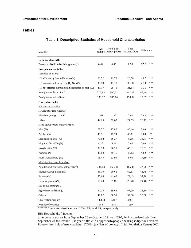
themselves poorer in 2006 than in 2000 (see Table 1).

2.2 Tropical Storm Stan and Precipitation Data

The main question of this research is to assess whether those who were affected by

Tropical Storm Stan have a higher likelihood of declaring themselves poorer in 2006 than in

2000. In the 2006 ENCOVI, households were also explicitly asked whether Stan had affected

them. Around 23.5% of the households in Guatemala declared they suffered some kind of loss or

damage due to the storm.

We use the following criteria to classify municipalities as affected by the storm. The

information was obtained from a report commissioned by the “Secretaría Nacional de

Planificación y Programación.” In the sample, 39.6% of the households lived in municipalities

considered affected. So, 60.4% of the households live in municipalities that were not considered

affected. Also, within the affected municipalities, there are people who declared that they were

not affected. They represent only 25.7% within the affected municipalities, which implies that


5

74.3% of the households in affected municipalities declared that they were affected by Stan (see

Table 1).

Climatic information on precipitation was collected from Climate Forecasting System

Reanalysis (CFSR) from simulation of the daily meteorological forecasting worldwide done by

the National Centers for Environmental Prediction (NCEP) (Saha et al. 2010). The average

precipitation for each municipality for the period when Stan affected them was calculated for

each municipality. We also calculate the accumulated typical precipitation before Stan for the

same period of the year that Stan hit (from September 28th to October 8th). We find that

precipitation significantly increased during Stan, as expected.

2.3 Poor versus Non-poor Municipalities

According to the 2002 Census, the national poverty rate was 55%. Within the poorer 50%

of municipalities in 2002, the average poverty rate was 79%. Within the 50% less poor

municipalities, poverty rates were also high, reaching an average of 41%. As can be seen in

Table 1, a higher fraction of indigenous people live in poor municipalities. Additionally, poor

municipalities are less densely populated and the most important economic sectors are

agriculture and fishing. These differences are statistically significant.

As also shown in Table 1, households in less poor municipalities declare being poorer in

2006 (46%) than they were in 2000 more often than households in poor municipalities (39%).

These differences are statistically significant. It is important to emphasize that poverty rates

capture poverty at one moment in time, while our dependent variable, being poorer in 2006 than

in 2000, captures change.

The likelihood of reporting being affected by Stan is larger in poor municipalities

(26.58%) than in less poor municipalities (21.7%). This shows that poor municipalities were

more exposed to Stan. This is consistent with the increases in precipitation shown in the period

and the fact that they depend more on agriculture and fishing. These differences are also

statistically significant. However, the percentage of households in the sample that live in affected

municipalities is larger in less poor municipalities. This might be explained by differences in

populations between affected and unaffected, and poor and less poor, municipalities.

Within affected municipalities, the percentage of households that declared that they were

not affected by Stan is significantly lower in poor municipalities than in less poor municipalities.

This also shows that Stan affected a larger percentage of households in poor municipalities than

in less poor municipalities, among the municipalities considered affected.


6

2.4 Control Variables

From the 2006 ENCOVI survey, we also obtained demographic variables for the head of

household, such as sex, age, level of education, and migration between 2000 and 2006. The

number of dependents in the household (people younger than 12 years) was also included. In

Table 1, we show that the differences between poor and less poor municipalities are significant

for every characteristic we use in the analysis.

Additionally, from the census, we have information about other socioeconomic

conditions at the municipality level for 2002. This allows us to control for initial socioeconomic

conditions at the aggregate level. Variables included at the municipality level were the

percentage of indigenous population and percentage of population in agriculture and fishing. In

Table 1, we can see that differences between poor and less poor municipalities are significant for

every characteristic we use in the analysis.

3. Empirical Strategy

In order to identify the effects of Stan on the likelihood of being poorer in 2006, we face

two challenges. The first challenge is identifying which households have been affected by the

storm. As explained before, studies that rely on self-reporting and use households that do not

report being affected as controls fail to account for the indirect effects of shocks. For instance,

impacts on infrastructure and the economy could indirectly negatively affect those individuals

within the community by, for example, reducing economic activity. However, when a shock

occurs, governments could also increase expenditures in relief efforts through social programs

and public investments in the areas affected (Cole et al. 2012; Besley and Burgess 2002).

Households that live in affected areas but were not affected could be better off than they would

have been if the shock had not occurred. As for papers that use municipality level data to identify

shocks, many of these studies relied on climatic information (as in Vicarelli 2010; Macours et al.

2012), with the result that households that were not directly affected by the shock, living in

affected municipalities, are classified as affected.1 As argued before, the level of impacts varies

among those indirectly affected, with some households better off due to the public investments

that follow the shock, and others worse off due to reduced economic activity. Distinguishing

these effects is not possible when using only municipality level data. For the reasons discussed

1 Similarly, de Janvry et al. (2006) use self-reported information but aggregate these reports at the community level

for the statistical analysis.


7

above, this issue might be even more important when estimating the differences in the effects

between poor and less poor households, especially if relief efforts are being targeted based on

poverty.

We address this issue using a combination of self-reported data and municipality level

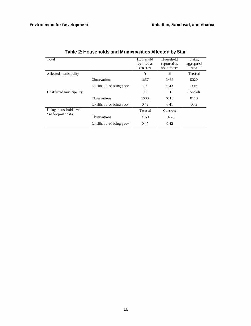
data. In Table 2, we classified households according to whether or not they live in a municipality

declared affected and whether or not they declared that they were affected. In Table 2, we show

households that reported being affected and that live in a municipality that was declared affected

(cell A), households that reported not being affected but live in a municipality that was declared

affected (cell B), households that reported being affected but live in a municipality that was

declared not affected (cell C), and households that reported not being affected and live in a

municipality that was declared not affected (cell D).

If we compared treated and controls using aggregated data (A and B versus C and D), we

would conclude that the effect is about a 4% increase in the likelihood of becoming poorer,

while, if we compared treated and controls using only self-reported data (A and C versus B and

D), we would conclude that the effect is about a 5% increase in the likelihood of becoming

poorer. However, those estimates are contaminated by observations in B. In the case of

aggregated data, observations in B affect the set of treated observations by reducing treated

average outcome levels. In the case of self-reported data, observations in B affect the set of

control observations by increasing control average outcome levels. A better estimate of the effect

would come from using only observations that were fully affected (cell A) versus observations

that were not affected in any form (cell D). We then would conclude that the effect is about a 9%

increase in the likelihood of becoming poorer.

We can see that, on average for the whole sample and using only aggregated data or only

self-reported data, households in B reduce the estimates of the impact. However, the direction of

the sign by which B can affect the estimations is uncertain and might vary depending on the sub-

sample analyzed. As we explained previously, households in B might be better or worse off after

the shock. In Table 3, we show how the values of B change drastically between poor

municipalities and less poor municipalities.

Moreover, we can estimate whether Stan and all its consequences had positive or

negative indirect effects on those households in cell B (those that declared themselves unaffected

in affected municipalities) by comparing outcomes in B against outcomes in D. We observe that

individuals in B in less poor municipalities might be worse off. However, individuals in B in

poor municipalities might be better off.


8

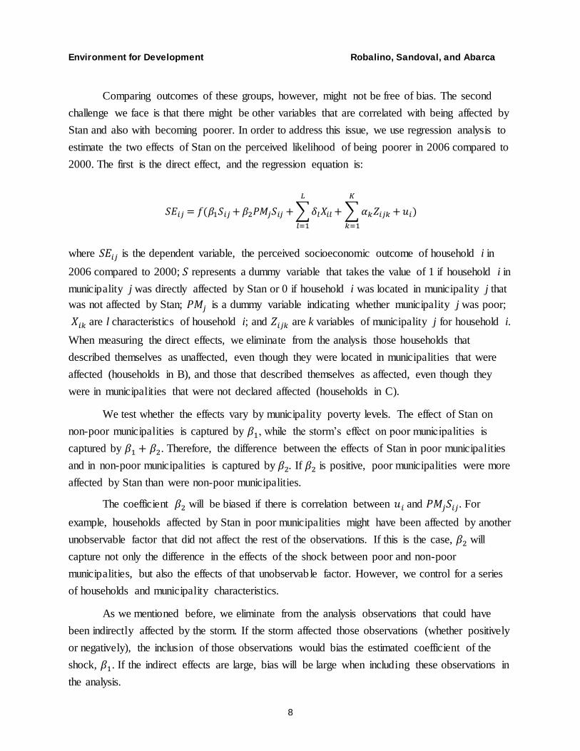
Comparing outcomes of these groups, however, might not be free of bias. The second

challenge we face is that there might be other variables that are correlated with being affected by

Stan and also with becoming poorer. In order to address this issue, we use regression analysis to

estimate the two effects of Stan on the perceived likelihood of being poorer in 2006 compared to

2000. The first is the direct effect, and the regression equation is:

𝑆𝐸𝑖𝑗 = 𝑓(𝛽1𝑆𝑖𝑗 + 𝛽2𝑃𝑀𝑗𝑆𝑖𝑗 + ∑ 𝛿𝑙𝑋𝑖𝑙

𝐿

𝑙=1

+ ∑ 𝛼𝑘𝑍𝑖𝑗𝑘

𝐾

𝑘=1

+ 𝑢𝑖)

where 𝑆𝐸𝑖𝑗 is the dependent variable, the perceived socioeconomic outcome of household i in

2006 compared to 2000; 𝑆 represents a dummy variable that takes the value of 1 if household i in

municipality j was directly affected by Stan or 0 if household i was located in municipality j that

was not affected by Stan; 𝑃𝑀𝑗 is a dummy variable indicating whether municipality j was poor;

𝑋𝑖𝑘 are l characteristics of household i; and 𝑍𝑖𝑗𝑘 are k variables of municipality j for household i.

When measuring the direct effects, we eliminate from the analysis those households that

described themselves as unaffected, even though they were located in municipalities that were

affected (households in B), and those that described themselves as affected, even though they

were in municipalities that were not declared affected (households in C).

We test whether the effects vary by municipality poverty levels. The effect of Stan on

non-poor municipalities is captured by 𝛽1, while the storm’s effect on poor municipalities is

captured by 𝛽1 + 𝛽2. Therefore, the difference between the effects of Stan in poor municipalities

and in non-poor municipalities is captured by 𝛽2. If 𝛽2 is positive, poor municipalities were more

affected by Stan than were non-poor municipalities.

The coefficient 𝛽2 will be biased if there is correlation between 𝑢𝑖 and 𝑃𝑀𝑗𝑆𝑖𝑗. For

example, households affected by Stan in poor municipalities might have been affected by another

unobservable factor that did not affect the rest of the observations. If this is the case, 𝛽2 will

capture not only the difference in the effects of the shock between poor and non-poor

municipalities, but also the effects of that unobservable factor. However, we control for a series

of households and municipality characteristics.

As we mentioned before, we eliminate from the analysis observations that could have

been indirectly affected by the storm. If the storm affected those observations (whether positively

or negatively), the inclusion of those observations would bias the estimated coefficient of the

shock, 𝛽1. If the indirect effects are large, bias will be large when including these observations in

the analysis.


9

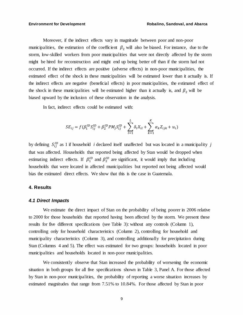
Moreover, if the indirect effects vary in magnitude between poor and non-poor

municipalities, the estimation of the coefficient 𝛽2 will also be biased. For instance, due to the

storm, low-skilled workers from poor municipalities that were not directly affected by the storm

might be hired for reconstruction and might end up being better off than if the storm had not

occurred. If the indirect effects are positive (adverse effects) in non-poor municipalities, the

estimated effect of the shock in these municipalities will be estimated lower than it actually is. If

the indirect effects are negative (beneficial effects) in poor municipalities, the estimated effect of

the shock in these municipalities will be estimated higher than it actually is, and 𝛽2 will be

biased upward by the inclusion of these observation in the analysis.

In fact, indirect effects could be estimated with:

𝑆𝐸𝑖𝑗 = 𝑓(𝛽1𝐼𝐷𝑆𝑖𝑗

𝐼𝐷 + 𝛽2𝐼𝐷𝑃𝑀𝑗𝑆𝑖𝑗

𝐼𝐷 + ∑𝛿𝑙𝑋𝑖𝑙

𝐿

𝑙=1

+ ∑ 𝛼𝑘𝑍𝑖𝑗𝑘

𝐾

𝑘=1

+ 𝑢𝑖)

by defining 𝑆𝑖𝑗𝐼𝐷 as 1 if household i declared itself unaffected but was located in a municipality j

that was affected. Households that reported being affected by Stan would be dropped when

estimating indirect effects. If 𝛽1𝐼𝐷 and 𝛽2

𝐼𝐷 are significant, it would imply that including

households that were located in affected municipalities but reported not being affected would

bias the estimated direct effects. We show that this is the case in Guatemala.

4. Results

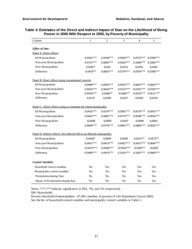
4.1 Direct Impacts

We estimate the direct impact of Stan on the probability of being poorer in 2006 relative

to 2000 for those households that reported having been affected by the storm. We present these

results for five different specifications (see Table 3): without any controls (Column 1),

controlling only for household characteristics (Column 2), controlling for household and

municipality characteristics (Column 3), and controlling additionally for precipitation during

Stan (Columns 4 and 5). The effect was estimated for two groups: households located in poor

municipalities and households located in non-poor municipalities.

We consistently observe that Stan increased the probability of worsening the economic

situation in both groups for all five specifications shown in Table 3, Panel A. For those affected

by Stan in non-poor municipalities, the probability of reporting a worse situation increases by

estimated magnitudes that range from 7.51% to 10.84%. For those affected by Stan in poor


10

municipalities, the estimates of the effects range from 2.4% to 3%, but most are not statistically

significant. Non-poor municipalities are significantly more affected than poor municipalities, as

can be seen in the last row of Panel A.

4.2 Biased Estimates

As discussed in the empirical section, if we had included households that reported not

being affected, despite being located in affected areas, the estimates would have been different

(see Table 3, Panel B). For non-poor municipalities, coefficients tend to be slightly lower,

ranging from 5.9% to 7.8%. For poor municipalities, the estimated effects are now positive and

significant, ranging from 3.6% to 5.1%. The differences between poor and non-poor

municipalities become insignificant.

If we had defined all households in affected municipalities as directly affected by the

storm, the estimates would also have been different (see Table 3, Panel C). For non-poor

municipalities, coefficients are also slightly lower, ranging from 6.4% to 9.3%. For poor

municipalities, however, the coefficients are insignificant and some of them become negative.

These results are slightly lower than the ones found in Panel A. However, these treatment effects

include households that were affected indirectly and these effects could be positive or negative.

The differences between poor and non-poor municipalities become significant, as can be seen in

the last row of Panel C.

4.3 Indirect Effects

To complement the analysis, we estimated indirect effects of Stan (see Table 3, Panel D).

We test whether those individuals in affected zones that reported not being affected were actually

affected. We find that, for non-poor municipalities, those households that live in affected

municipalities, but reported not being affected directly, have a higher probability of reporting a

worse situation. The estimates of the increment in that probability range from 4.3% to 6.4%.

These results are all statistically significant. This is consistent with our previous discussion about

the fact that including these observations will likely bias the coefficients downward.

However, in poor municipalities, the opposite occurs. Those individuals in households

that were not affected, in municipalities that were affected, were better off after the occurrence of

the event. The probability of reporting a worst situation decreases. This reduction ranges from

3.29% to 5.63%. The government might have increased anti-poverty programs in the places that

were hit by the storm. Reconstruction efforts might especially benefit the poor because the

demand for low-skilled labor increases. Whatever the reason for this finding, it is important to


11

emphasize that the inclusion of indirectly affected households as if they were not affected will

bias the estimates of the impacts, as shown in Table 3, Panels B and C. The difference between

the impacts in poor and non-poor municipalities will also be biased.

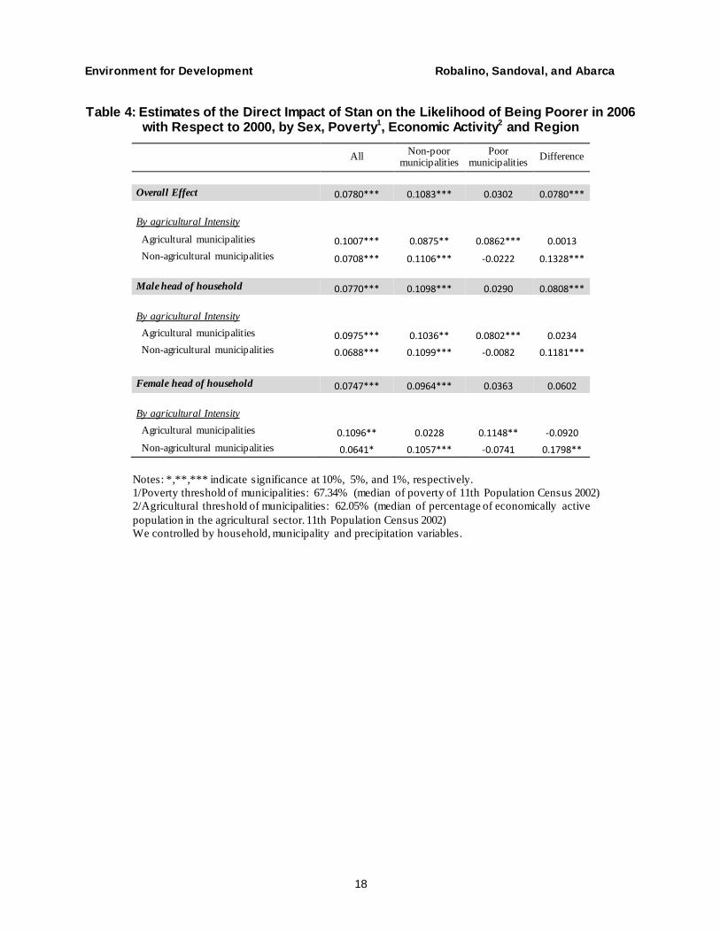
4.4 Agricultural Intensity and Gender Differences

We then split the sample of municipalities according to the intensity in agriculture2 and

by the head of household’s gender. We find that, in agricultural municipalities, there is no

statistically significant difference between the direct effects on households living in poor and

non-poor municipalities (see Table 4). This result holds when we use the entire sample and when

we use only male or female heads of households. The magnitudes of these effects are similar for

households living in both poor and non-poor agricultural municipalities when using the entire

sample and when focusing on households headed by males. For households headed by females,

the impact seems to be larger for those living in poor municipalities; however, the effect is not

statistically significant.

We also find that the direct effects differ significantly in non-agricultural municipalities

between poor and non-poor municipalities. Households in poorer municipalities are significantly

less affected. This might be the result of government assistance that is targeting the poor. This

could also be explained by the fact that households in poor municipalities have few assets and

little to lose. These results were robust to head of household gender.

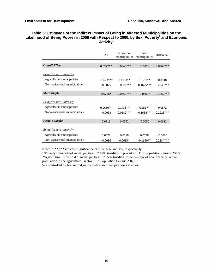
In non-poor municipalities, the indirect effects of Stan on the likelihood of reporting

becoming poorer were positive and significant, especially in agricultural municipalities (see

Table 5). The magnitude of the adverse effects in poor agricultural municipalities was also

positive and significant. However, the indirect effects of Stan in poor and non-agricultural

municipalities were negative and significant. Households that were in an affected municipality

but reported not being affected by the shock are significantly better off than they would have

been if the shock had not occurred.

2 We use the 2002 census information about individuals’ economic activity. The median is 63% participation in

agriculture. If 63% or more of the individuals in a municipality work in agriculture, the municipality is classified as

an agricultural municipality; if less than 63% work in agriculture, the municipality is classified as a non -agricultural

municipality.


12

5. Conclusions

Extreme weather events have increased in intensity and frequency. The literature

analyzing the effects of these events on social and economic outcomes has increased

significantly. Most previous analyses use either self-reported data about being affected, or

aggregated data such as precipitation at the municipality level. In this paper, we argue that these

estimates might be biased due to the presence of indirect effects. In studies that use self-reported

data, households indirectly affected are used as controls, while in aggregated level data,

households indirectly affected are part of the treated observations.

Using data for Guatemala, we estimated separately the direct and indirect effects of

Tropical Storm Stan on subjective economic well-being. We found that households that were

directly affected by Stan have a significantly higher likelihood of reporting being poorer after the

event. We also found that the indirect effects can be positive or negative. For non-poor

municipalities, households that reported being unaffected by the storm, despite living in an

affected municipality, have a significantly higher likelihood of reporting being poorer in 2006

relative to 2000. For poor municipalities, households that reported not being affected by the

storm, despite living in an affected municipality, have a significantly lower likelihood of

reporting being poorer in 2006 relative to 2000. This might be explained, for instance, by the

redirection of government resources toward poorer affected communities.

Given that shocks and responses to shocks will likely affect households not directly

exposed, estimates of the effects of extreme weather events on social outcomes are difficult to

measure. Without considering exposure data at both household level and municipality level

simultaneously, estimates of impacts might be biased because they will capture the effects of

responses to shocks over the population.


13

References

Baez, J., and I. Santos. 2007. Children’s Vulnerability to Weather Shocks: A Natural Disaster as

a Natural Experiment. Social Science Research Network, New York.

Besley, T., and R. Burgess. 2002. The Political Economy of Government Responsiveness:

Theory and Evidence from India. The Quarterly Journal of Economics 117(4): 1415-

1451.

Bustelo, M. 2011. Three Essays on Investments in Children’s Human Capital. Submitted in

Partial Fulfillment of the Requirements for the Degree of Doctor of Philosophy in

Agricultural and Applied Economics in the Graduate College of the University of Illinois

at Urbana Champaign.

Carter, M.R., P.D. Little, T. Mogues, and W. Negatu. 2007. Poverty Traps and Natural Disasters

in Ethiopia and Honduras. World Development 35(5): 835-856.

CCAD and SICA. 2011. Estrategia Regional de Cambio Climático: Comisión Centroamericana

de Ambiente y Desarrollo (CCAD). Sistema de la Integración Centroamericana (SICA).

Cole, S., A. Healy, and E. Werker. 2012. Do Voters Demand Responsive Governments?

Evidence from Indian Disaster Relief. Journal of Development Economics 97(2): 167-

181.

De Janvry, A. et al. 2006. Can Conditional Cash Transfer Programs Serve as Safety Nets in

Keeping Children at School and from Working When Exposed to Shocks? Journal of

Development Economics 79.2(2006): 349-373.

ECLAC. 2005. Efectos en Guatemala de las Lluvias Torrenciales y la Tormenta Tropical Stan.

Octubre de 2005.

ECLAC. 2010. La Economía del Cambio Climático en Centroamérica: Naciones Unidas,

Comisión Económica para America Latina y el Caribe. Comisión Centroamericana de

Ambiente y Desarrollo.

ECLAC. 2012. La Economía del Cambio Climático en Centroamérica: Naciones Unidas,

Comisión Económica para America Latina y el Caribe. Comisión Centroamericana de

Ambiente y Desarrollo.

Gitter, S. 2005. Conditional Cash Transfers, Credit, Remittances, Shocks, and Education: An

Impact Evaluation of Nicaragua’s RPS. University of Wisconsin-Madison, Department of

Agricultural and Applied Economics.


14

Herrera, J.L. 2003. Estado Actual del Clima y la Calidad Del Aire en Guatemala Guatemala:

Instituto de Incidencia Ambiental. Universidad Rafael Landívar, Facultad de Ciencias

Ambientales y Agrícolas, Instituto de Agricultura, Recursos Naturales y Agrícolas.

Maluccio, J.A. 2005. Coping with the “Coffee Crisis" in Central America: The Role of the

Nicaraguan Red de Protección Social. Washington, DC: IFPRI

Macours, K., Premand, P., and Vakis, R. 2012. Transfers, diversification and household risk

strategies: experimental evidence with lessons for climate change adaptation. World

Bank Policy Research Working Paper 6053.

Mendelsohn, R. 2012. The Economics of Adaptation to Climate Change in Developing

Countries. Climate Change Economics 3(02): 1250006.

Morduch, J. 1994. Poverty and Vulnerability. The American Economic Review 84: 221-225.

Ospina, M. 2011. CCT Programs for Consumption Insurance: Evidence from Colombia

Universidad EAFIT.

Rosemberg, C., R. Fort, and M. Glave. 2010. Efecto que Tienen los Desastres Naturales en las

Transiciones Entre Estados de Pobreza y en el Crecimiento Del Consumo. Evidencias al

Respecto en Zonas Rurales de Perú. Bienestar y Politica Social 6(1): 59-98.

Rosenzweig, M.R., and H.P. Binswanger. 1993. Wealth, Weather Risk, and the Composition and

Profitability of Agricultural Investments Vol. 1055. World Bank Publications.

Saha, S. et al. 2010. The NCEP Climate Forecast System Reanalysis. Bulletin of the American

Meteorological Society 91(8): 1015-1057.

Skoufias, E. 2003. Economic Crises and Natural Disasters: Coping Strategies and Policy

Implications. World Development 31(7): 1087-1102.

Strobl, E. 2011. The Economic Growth Impact of Hurricanes: Evidence from US Coastal

Counties. Review of Economics and Statistics 93(2): 575-589.

UNICEF. 2010. Guatemala la Tormenta Perfecta. Impacto del Cambio Climático y la Crisis

Económica en la Niñez y la Adolescencia: Fondo de las Naciones Unidas para la

Infancia.

Vicarelli, M. 2010. Exogenous Income Shocks and Consumption Smoothing Strategies among

Rural Households in Mexico. Center for International Development, Harvard Kennedy

School.

World Bank. 2009. Guatemala Poverty Assessment: Good Performance at Low Levels.


15

Tables

Table 1: Descriptive Statistics of Household Characteristics

Variables

All sample

Non-Poor Municipalities

Poor Municipalities

Difference

Dependent variable

Perceived likelihood of being poorer(f) 0,44 0,46 0,39 6,52 ***

Independent variables

Variables of interest

HH affected by Stan self-report (%) 23,52 21,70 26,58 4,87 ***

HH in municipalities affected by Stan (%) 39,59 41,18 36,88 4,30 ***

HH not affected in municipalities affected by Stan (%) 25,77 28,49 21,14 7,35 ***

Precipitation during Stana 317,93 300,72 347,13 46,40 ***

Precipitation before Stanb

189,92 185,14 198,02 12,87 ***

Control variables HH control variables Household characteristics Members younger than 12 1,61 1,37 2,01 0,63 ***

Urban 42,25 52,67 24,55 28,12 ***

Head of household characteristics Men (%) 78,77 77,80 80,40 2,60 ***

Age (years) 45,51 45,74 45,11 0,63 **

Spanish speakingc (%) 71,92 86,27 47,56 38,71 ***

Migrate 2001-2006 (%) 4,25 5,21 2,60 2,60 ***

No education (%) 33,53 26,29 45,81 19,51 ***

Primary (%) 48,04 49,75 45,13 4,62 ***

More than primary (%) 18,43 23,94 9,05 14,89 ***

Municipality control variables Population density (# people per Km

2) 484,64 660,88 185,40 475,48 ***

Indigenous population (%) 36,10 20,62 62,37 41,75 ***

Poverty (%) 55,66 41,65 79,43 37,78 ***

Extreme poverty (%) 15,28 7,31 28,78 21,46 ***

Economic sector (%): Agriculture and fishing 50,18 39,68 67,99 28,30 ***

Others 49,82 60,31 32,00 28,30 ***

Observation number 13.438 8.457 4.981 Number of counties 288 149 139 *,**,*** indicate significance at 10%, 5%, and 1%, respectively.

HH: Households, f: fraction.

a/ Accumulated rain from September 28 to October 10 in year 2005; b/ Accumulated rain from

September 28 to October 10 in year 2004; c/ As opposed to people speaking indigenous dialects

Poverty threshold of municipalities: 67.34% (median of poverty of 11th Population Census 2002)


16

Table 2: Households and Municipalities Affected by Stan

Total Household

reported as

affected

Household

reported as

not affected

Using

aggregated

data

Affected municipality A B Treated

Observations 1857 3463 5320

Likelihood of being poor 0,5 0,43 0,46

Unaffected municipality C D Controls

Observations 1303 6815 8118

Likelihood of being poor 0,42 0,41 0,42

Using household level

“self-report” data

Treated Controls

Observations 3160 10278

Likelihood of being poor 0,47 0,42


17

Table 3: Estimates of the Direct and Indirect Impact of Stan on the Likelihood of Being Poorer in 2006 With Respect to 2000, by Poverty of Municipality

Column 1 2 3 4 5

Effect of Stan

Panel A: Direct effects

All Municipalities 0.0542*** 0.0538*** 0.0569*** 0.0772*** 0.0780***

Non-poor Municipalities 0.0751*** 0.0845*** 0.0932*** 0.1084*** 0.1083***

Poor Municipalities 0.0281* 0,024 0,0153 0,0291 0,0302

Difference 0.0470** 0.0605*** 0.0779*** 0.0793*** 0.0780***

Panel B: Direct effects using contaminated controls



Poor Municipalities 0.0418*** 0.0368** 0.0384** 0.0516*** 0.0511***

Difference 0,0176 0,0296 0,0337 0,0264 0,0234

Panel C: Direct effects using as treatment the whole municipality



Poor Municipalities -0,0048 -0,0095 -0,0187 -0,0048 0,0001

Difference 0.0690*** 0.0776*** 0.0961*** 0.0986*** 0.0935***

Panel D: Indirect effects: Not affected HH in an affected municipality

All Municipalities 0.0183* 0,0094 0,0049 0.0237** 0.0272**


Poor Municipalities -0.0474*** -0.0506*** -0.0563*** -0.0387** -0,0329

Difference 0.0906*** 0.0919*** 0.1014*** 0.1001*** 0.0969***

Control Variables

Household control variables No Yes Yes Yes Yes

Municipality control variables No No Yes Yes Yes

Precipitation during Stan No No No Yes Yes

Square of Precipitation during Stan No No No No Yes

Notes: *,**,*** indicate significance at 10%, 5%, and 1% respectively.

HH: Households

Poverty threshold of municipalities: 67.34% (median of poverty of 11th Population Census 2002)

See the list of household control variables and municipality control variables in Table 1.


18

Table 4: Estimates of the Direct Impact of Stan on the Likelihood of Being Poorer in 2006 with Respect to 2000, by Sex, Poverty1, Economic Activity2 and Region

All Non-poor

municipalities Poor

municipalities Difference

Overall Effect 0.0780*** 0.1083*** 0.0302 0.0780***

By agricultural Intensity

Agricultural municipalities 0.1007*** 0.0875** 0.0862*** 0.0013

Non-agricultural municipalities 0.0708*** 0.1106*** -0.0222 0.1328***

Male head of household 0.0770*** 0.1098*** 0.0290 0.0808***


Agricultural municipalities 0.0975*** 0.1036** 0.0802*** 0.0234

Non-agricultural municipalities 0.0688*** 0.1099*** -0.0082 0.1181***

Female head of household 0.0747*** 0.0964*** 0.0363 0.0602


Agricultural municipalities 0.1096** 0.0228 0.1148** -0.0920

Non-agricultural municipalities 0.0641* 0.1057*** -0.0741 0.1798**

Notes: *,**,*** indicate significance at 10%, 5%, and 1%, respectively.

1/Poverty threshold of municipalities: 67.34% (median of poverty of 11th Population Census 2002)

2/Agricultural threshold of municipalities: 62.05% (median of percentage of economically active

population in the agricultural sector. 11th Population Census 2002)

We controlled by household, municipality and precipitation variables.


19

Table 5: Estimates of the Indirect Impact of Being in Affected Municipalities on the Likelihood of Being Poorer in 2006 with Respect to 2000, by Sex, Poverty1 and Economic

Activity2

All Non-poor

municipalities

Poor

municipalities Difference

Overall Effect 0.0272** 0.0640*** -0.0329 0.0969***


Agricultural municipalities 0.0673*** 0.1131** 0.0613** 0.0518

Non-agricultural municipalities -0.0025 0.0622*** -0.1625*** 0.2246***

Male sample 0.0268* 0.0652*** -0.0400* 0.1052***


Agricultural municipalities 0.0660** 0.1438*** 0.0567* 0.0872

Non-agricultural municipalities -0.0033 0.0589*** -0.1634*** 0.2223***

Female sample 0.0215 0.0562 -0.0050 0.0612


Agricultural municipalities 0.0677 0.0258 0.0788 -0.0530

Non-agricultural municipalities -0.0086 0.0685* -0.1650** 0.2334***

Notes: *,**,*** indicate significance at 10%, 5%, and 1%, respectively.

1/Poverty threshold of municipalities: 67.34% (median of poverty of 11th Population Census 2002).

2/Agricultural threshold of municipalities: 62.05% (median of percentage of economically active

population in the agricultural sector. 11th Population Census 2002).

We controlled by household, municipality and precipitation variables.

Documents

Direct and Indirect Effects of Extreme Weather Events and