Direct and Indirect Effect of Depression in Adolescence on Adult Wages

Meliyanni Johar* & Jeffrey Truong

University of Technology Sydney, Australia

* Corresponding author: Associate Professor. Economics Discipline Group. University of

Technology Sydney. PO BOX 123 Broadway NSW 2007 Australia. T: +612 95147742. F: +612 95147722. E: Meliyanni.Johar@uts.edu.au

2

Abstract

It is well recognised that a depressive mental state can persist for a long

time, and this can adversely impact labour market outcomes. The aim of

this paper is to examine the direct association between depression

status in late-teenage years and adult wages, as well as the indirect

association, operating though accumulated education, experience and

occupation choice. Using the National Longitudinal Survey of Youth

1997 data, we find adolescent depression is associated with a wage

penalty of around 10-15%, but its mechanics are very different for

males and females. For males, about three quarters of the wage penalty

is through the direct channel, whilst for females the indirect effect

channel is dominant. The indirect channel is driven by lower

accumulated education, mostly because depression discourages further

study post high school. These results are important because they imply

that the association between adolescent depression and wages is

stronger than has been estimated in previous cross-sectional studies.

Keywords: Adolescence depression, early onset depression, wages, human capital accumulation

JEL Codes: J24, I15

3

1. Introduction

Regarded as one of major the hidden health burdens in the 21st century by the World Health

Organization (WHO), depression has been estimated as the world’s second leading cause of

disability in terms of total years lost since the start of the current decade (Ferrari et al. 2013). It

has been projected by 2020 that depression will only be ranked second to cardiovascular

disease in terms of being the largest contributor to the global health burden (Murray & Lopez

1996). The economic impact of depression has been found to be mainly due to labour market

outcomes, in particular, loss of productivity in the workplace. In the US, approximately 10% of

the population who are aged above 18 meet the clinical criteria for depression, and the annual

economic cost of the illness for U.S. has been estimated to be $83.1 billion with approximately

60% attributed to the loss of productivity in the workplace (Greenberg et al., 2003).

Depression can be a chronic condition that persists over many years. Depression during

adolescence for instance may extend to adulthood and impact on labour market outcomes. Early

onset depression may also affect personal traits, and as it takes place within the lifecycle phase

of individuals that is primarily marked by the formation of critical human capital such as

education, early onset depression may impede labour market successes by lowering an

individual’s human capital accumulation. However, very few studies examine the impact of

adolescent depression on labour market outcomes in adulthood. Furthermore, the few existing

studies do not explicitly test for the ‘indirect’ effect from channels through which adolescent

depression may operate, such as the lower educational attainment. The direct effect is often the

sole focus, while the total effect of adolescent depression on labour market outcomes may be

substantially bigger if these indirect effects are large. The aim of this study is to fill this void in

the literature by estimating the total effect of adolescent depression, accounting for the size of

the direct as well as indirect effects that may operate through accumulated education, work

experience and occupational type. Our approach adapts from the framework of Han et al.

(2011), which quantifies the direct and indirect effects of adolescent body mass index on adult

wages. We are cautious, however, in claiming causal inference, which relies on the presence of

instrumental variables that affect depression during adolescence but have no impact on any of

the mediating channels. In the absence of experiments (e.g., random lottery), such variables are

almost impossible to find, forcing researchers to compromise with assumptions that may create

a larger bias than ignoring endogeneity in the first place.1 Nevertheless, any knowledge about

1 See Murray (2006) for a discussion of weak instrumental variables. To our knowledge, there has not been any technical paper which estimates the causal effects of multiple mediators. Several papers have

4

the various pathways through which adolescent depression may operate is valuable in

developing efficacious policy to lower the economic cost of depression.

Depression during adolescent years may adversely impact labour market outcomes because

depressed individuals may have achieved lower levels of education. Studies have linked

depression with higher drop-out rates and lower grades (Roeser et al., 1998; Asarnow et al.

2005; Quiroga et al. 2013). In turn lower education may impact on job opportunities to be

employed in high wage jobs. Adolescent depression may also reduce labour market attachment,

resulting in lower levels of work experience (Kaplan 2012; Sands, 2008). This in turn may also

limit the chance to be employed in higher paying jobs. There is also evidence that adolescent

depression has a direct impact on adult labour market outcomes. Depressed youths may be

more likely to develop undesirable psychiatric behaviours such as mood swings, dullness, and

pessimism that may limit their career progression later. On the other end, employers and work

colleagues may find it more difficult to give promotion or valuable projects in the presence of

such behaviours. Fletcher (2013) regresses adult annual earnings on adolescent depression and

finds that adolescent depression reduces adult earnings by approximately 15%. When the

current depression state is also included in the regression, this adolescent depression

coefficient remain significant and is only reduced by about 4 percentage point, suggesting that

adolescent depression has a lasting, independent impact on future labour market outcome, even

if the individual has got out from the depressive state.

We use data from the the National Longitudinal Survey of Youth 1997 (NLSY97), which is a

nationally representative of American youths aged between 13 and 17 in 1997. We have

information about the condition of their mental health condition when they were aged 16 to 21

(wave 4 (2000) and wave 6 (2004)) and their characteristics as adults ten years later (wave 14

(2010) and wave 15 (2011)). There are four outcome variables in adulthood, which are wage,

accumulated education level (total years of schooling and tertiary education), accumulated

work experience and job category. We estimate separate models for males and females because

it is widely known that they have very distinct labour market behaviours. Our estimates indicate

that both the magnitude and composition of the total effect for the depression wage penalty are

different between genders. We find the total effect is larger in males at about 15% while in

females it is 10%. For males, about three quarters of the total effect is direct, whilst for females

focused on one mediator (e.g., Frolich and Huber, 2014), thereby assuming there is no other main mediator. This implicit assumption in turn makes the “direct” effect in their set up difficult to interpret as it also captures the indirect effects of other main mediators that are not explicitly considered in estimation.

5

the indirect effects tend to dominate. The large indirect effect is found to be driven by lower

educational attainment. Non-trivial indirect effects imply that previous focus on direct effects

has underestimated the total effect of adolescent depression on wages. More importantly for

policymakers, the large indirect effects through education suggests that there is scope for

assistance programs or support groups in schools and tertiary institutions to dampen the

adverse impact of depression on educational progress.

2. Literature Review

Many educational outcomes have been negatively linked to adolescent depression. Using a

sample of 1041 adolescents from Maryland, Roeser et al. (1998) finds that depressive

symptoms lower grade-point average and increase the frequency of skipping classes. Quiroga et

al. (2013) finds that adolescents with depression are 2.75 times more likely to drop out of high

school. The impacts of adolescent depression on educational outcomes are more significant in

females. Ding et al. (2006) utilises a novel method of incorporating DNA information to control

for individual hereditary factors that may affect both education attainment and wages to

estimate the relationship between educational outcomes and adolescent depression. The study

finds that females with adolescent depression on average have a GPA lower than their non-

depressed counterparts, and lower than male adolescents with similar levels of depression.

Fletcher (2010) also finds similar effects for females but adds that adolescent depression also

reduces the likelihood of college completion for females. Such disparity in the effect of

depression on reduced educational attainment between genders has been attributed to females

being more biologically vulnerable to the effects of the depression than males (Piccinelli and

Wilkinson, 2000).

Despite a rich set of literature linking adolescent depression and reduced educational

attainment, few papers have examined how adolescent depression impacts labour market

outcomes in adulthood. Berndt et al. (2000) is one of the few studies to explore such link.

Information on education and the presence and severity of depressive symptoms during

adolescence are collected from 531 randomised individuals who are currently (age 30)

undergoing outpatient treatments for chronic depression, while the wage information is

obtained from the 1995 US Census Bureau’s Current Population survey. Similar to Fletcher

(2010) and Ding et al. (2006), they find that only females who suffered from adolescent

depression display significant reduction in educational attainment. Then using education, age

and gender as matching variables between the two data sources, the study predicts a wage

6

penalty from 12% at age 21 and progressively peaked to 18% at age 55 for a female who has

experienced depression as adolescence. Fletcher (2013) employs the National Longitudinal

Study of Adolescent Health (Add Health 1994/5) dataset, which is nationally representative of

of adolescents in grades 7-12 in the US, to estimate the impact of adolescent depression on

employment and annual income (earnings). He estimates OLS, school fixed-effect and family

fixed-effect models, and finds that in all specifications, adolescent depression negatively impacts

employment and earnings. The size of the effect is similar in all three models, suggesting small

role of fixed effects. The impact is reduced, but still significant, when education is controlled for,

suggesting that education is a potential mediator of the labour market penalty. For a Swedish

sample, Lunborg et al. (2014) shows that among various types of major health conditions,

mental conditions have the strongest effects on future outcomes.

Sands (2008) suggests that work experience, which is another form of human capital, may be

another pathway in which depression during adolescence may affect wages later in adulthood.

In addition to education, she examines the relationship between adolescent depression and

work experience. Unexpectedly, she finds a positive relationship. She then analyses how returns

to earnings from education and experience may vary by depression levels. Both education and

experience have positive returns, but the return from work experience is found to be larger for

those who experienced severe depression during adolescence. The loss of work experience due

to adolescent depression may also come from lower employment probability of those who

suffered from adolescent depression (Fletcher 2013; Kaplan 2012).

Occupation type may also explain wage differentials. The mental health literature has linked

depression with undesirable personality traits and deficits in emotional intelligence and social

skills that may persist well into adulthood. Jylhä et al. (2009) explores the relationship between

depression and the Big Five personality traits, and find that depressed individuals are more

likely to display traits of neuroticism and introversion. Karsten et al. (2012) finds that

depression is linked to increased introversion and neuroticism, and that these traits persist

even after recovery from depression. Studies on the relationship between personality traits and

earnings have suggested that emotional stability and extraversion are positively linked to

higher occupation status and earnings (e.g., Jokela and Keltikangas-Järvinen 2011; Mueller and

Plug 2006). This alludes to the possibility that adolescent depression has a direct impact on

outcomes in adulthood through personal characteristics (e.g. loss of social skills).

7

Adolescent depression may carry through to adulthood. Fergusson et al. (2007) explores the

recurrence of depression using 25 year longitudinal data of 982 New Zealand adolescents. The

study predicts that those who experienced 10 or more episodes of depression between 16-21

years of age were between 3 to 10 times more likely to experience it again by age 21-25 than

those who have not experienced it at all. Fombonne et al. (2001) also find similar trends

suggesting those who have experienced depression during adolescence will have a 50% chance

to experience it again by age 30. Depression in turn is linked to negative labour market

outcomes such as higher rates of absenteeism and reduced productivity. Adler et al. (2006)

explore the work performance of adults with depression and find that depressed workers had

significant deficits in managing output, time and interpersonal tasks compared to healthy or

moderately physically impaired workers. A two yearlong study conducted by Beck et al. (2011)

quantifies the loss of productivity from depression averaging up to approximately 2 days lost

per month. Wang et al. (2004) also posits the loss of productivity equivalent to a monthly 2 days

lost and monetised the income loss resulting from reduced productivity to $300 per month.

Frijters et al. (2010) find robust evidence that worse mental health has a substantial negative

impact on the probability of actively participating in the labour market, especially for females.

Indeed, the link between later outcomes and mental health status earlier in life can trace back to

mental health problems during childhood. Using attention deficit hyperactivity disorder (ADHD)

as a case of mental disabilities, Currie and Stabile (2006, 2007) find that children aged around

4-12 years old with ADHD have lower test scores than others (including their own siblings) and

are more likely to be placed in special education, to repeat grades, and to be delinquent. Their

studies utilize panel data which follow these children for over 10 years. Similarly, Smith (2009)

finds that general health status during childhood (up to age 16), which is strongly negatively

affected by depression, has negative impacts on the level of financial resources at the beginning

of the adult years around age 25 and its growth with age. Part of these impacts is due to reduced

work effort as poorer childhood health is transmitted into poorer adult health.

Previous studies have focused on the direct effect of adolescent depression by regressing labour

market outcomes in adulthood on adolescent depression, controlling for other factors including

education and current depression status (Fletcher 2013; Kaplan 2012). The model with current

depression status however is difficult to interpret due to reverse causality arising from a lower

wage increases the likelihood of depressive state. More importantly, as depression may also

affect human capital accumulation and occupation type, the coefficient for adolescent

depression from these models do not capture the indirect effect. The aim of this study is to

extend the literature by explicitly estimating the size and significance of the indirect effects of

8

depression during adolescence on labour market outcome many years later. Three specific

indirect channels are investigated: educational attainment, accumulated work experience and

occupation choice.

3. Methodology

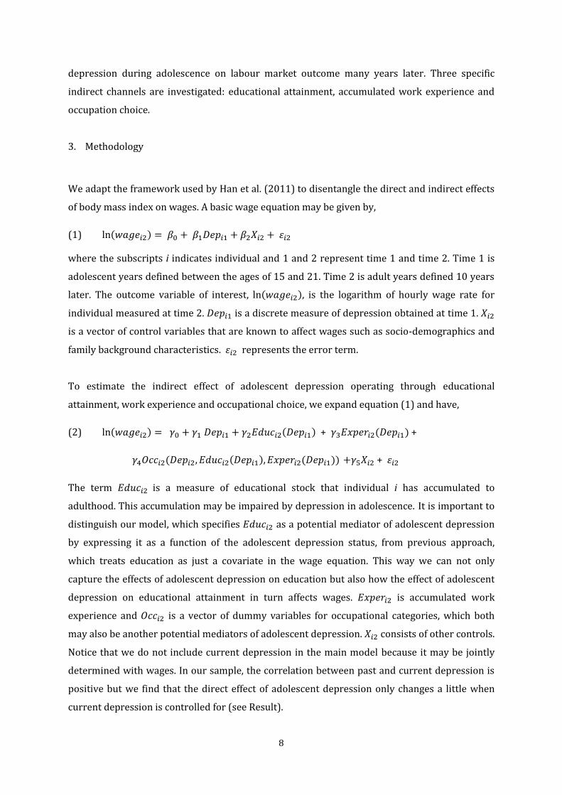
We adapt the framework used by Han et al. (2011) to disentangle the direct and indirect effects

of body mass index on wages. A basic wage equation may be given by,

(1) ln(𝑤𝑎𝑔𝑒𝑖2) = 𝛽0 + 𝛽1𝐷𝑒𝑝𝑖1 + 𝛽2𝑋𝑖2 + 𝜀𝑖2

where the subscripts i indicates individual and 1 and 2 represent time 1 and time 2. Time 1 is

adolescent years defined between the ages of 15 and 21. Time 2 is adult years defined 10 years

later. The outcome variable of interest, ln(𝑤𝑎𝑔𝑒𝑖2), is the logarithm of hourly wage rate for

individual measured at time 2. 𝐷𝑒𝑝𝑖1 is a discrete measure of depression obtained at time 1. 𝑋𝑖2

is a vector of control variables that are known to affect wages such as socio-demographics and

family background characteristics. 𝜀𝑖2 represents the error term.

To estimate the indirect effect of adolescent depression operating through educational

attainment, work experience and occupational choice, we expand equation (1) and have,

(2) ln(𝑤𝑎𝑔𝑒𝑖2) = 𝛾0 + 𝛾1 𝐷𝑒𝑝𝑖1 + 𝛾2𝐸𝑑𝑢𝑐𝑖2(𝐷𝑒𝑝𝑖1) + 𝛾3𝐸𝑥𝑝𝑒𝑟𝑖2(𝐷𝑒𝑝𝑖1) +

𝛾4𝑂𝑐𝑐𝑖2(𝐷𝑒𝑝𝑖2, 𝐸𝑑𝑢𝑐𝑖2(𝐷𝑒𝑝𝑖1), 𝐸𝑥𝑝𝑒𝑟𝑖2(𝐷𝑒𝑝𝑖1))-+𝛾5𝑋𝑖2 + 𝜀𝑖2

The term 𝐸𝑑𝑢𝑐𝑖2 is a measure of educational stock that individual i has accumulated to

adulthood. This accumulation may be impaired by depression in adolescence. It is important to

distinguish our model, which specifies 𝐸𝑑𝑢𝑐𝑖2 as a potential mediator of adolescent depression

by expressing it as a function of the adolescent depression status, from previous approach,

which treats education as just a covariate in the wage equation. This way we can not only

capture the effects of adolescent depression on education but also how the effect of adolescent

depression on educational attainment in turn affects wages. 𝐸𝑥𝑝𝑒𝑟𝑖2 is accumulated work

experience and 𝑂𝑐𝑐𝑖2 is a vector of dummy variables for occupational categories, which both

may also be another potential mediators of adolescent depression. 𝑋𝑖2 consists of other controls.

Notice that we do not include current depression in the main model because it may be jointly

determined with wages. In our sample, the correlation between past and current depression is

positive but we find that the direct effect of adolescent depression only changes a little when

current depression is controlled for (see Result).

9

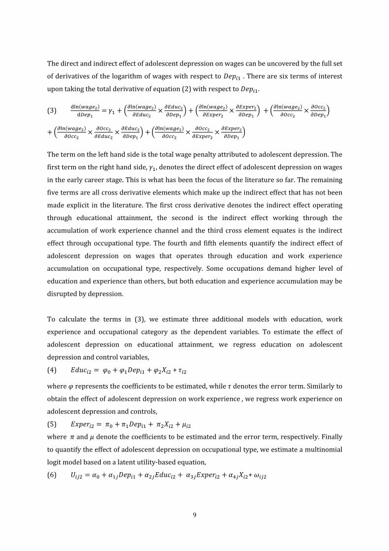
The direct and indirect effect of adolescent depression on wages can be uncovered by the full set

of derivatives of the logarithm of wages with respect to 𝐷𝑒𝑝𝑖1 . There are six terms of interest

upon taking the total derivative of equation (2) with respect to 𝐷𝑒𝑝𝑖1.

(3) dln(𝑤𝑎𝑔𝑒2)

d𝐷𝑒𝑝1= 𝛾1 + (

∂ln(𝑤𝑎𝑔𝑒2)

∂𝐸𝑑𝑢𝑐2×

∂𝐸𝑑𝑢𝑐2

∂𝐷𝑒𝑝1) + (

∂ln(𝑤𝑎𝑔𝑒2)

∂𝐸𝑥𝑝𝑒𝑟2×

∂𝐸𝑥𝑝𝑒𝑟2

∂𝐷𝑒𝑝1) + (

∂ln(𝑤𝑎𝑔𝑒2)

∂𝑂𝑐𝑐2×

∂𝑂𝑐𝑐2

∂𝐷𝑒𝑝1)

+ (∂ln(𝑤𝑎𝑔𝑒2)

∂𝑂𝑐𝑐2×

∂𝑂𝑐𝑐2

∂𝐸𝑑𝑢𝑐2×

∂𝐸𝑑𝑢𝑐2

∂𝐷𝑒𝑝1) + (

∂ln(𝑤𝑎𝑔𝑒2)

∂𝑂𝑐𝑐2×

∂𝑂𝑐𝑐2

∂𝐸𝑥𝑝𝑒𝑟2×

∂𝐸𝑥𝑝𝑒𝑟2

∂𝐷𝑒𝑝1)

The term on the left hand side is the total wage penalty attributed to adolescent depression. The

first term on the right hand side, 𝛾1, denotes the direct effect of adolescent depression on wages

in the early career stage. This is what has been the focus of the literature so far. The remaining

five terms are all cross derivative elements which make up the indirect effect that has not been

made explicit in the literature. The first cross derivative denotes the indirect effect operating

through educational attainment, the second is the indirect effect working through the

accumulation of work experience channel and the third cross element equates is the indirect

effect through occupational type. The fourth and fifth elements quantify the indirect effect of

adolescent depression on wages that operates through education and work experience

accumulation on occupational type, respectively. Some occupations demand higher level of

education and experience than others, but both education and experience accumulation may be

disrupted by depression.

To calculate the terms in (3), we estimate three additional models with education, work

experience and occupational category as the dependent variables. To estimate the effect of

adolescent depression on educational attainment, we regress education on adolescent

depression and control variables,

(4) 𝐸𝑑𝑢𝑐𝑖2 = 𝜑0 + 𝜑1𝐷𝑒𝑝𝑖1 + 𝜑2𝑋𝑖2 + 𝜏𝑖2

where 𝜑 represents the coefficients to be estimated, while 𝜏 denotes the error term. Similarly to

obtain the effect of adolescent depression on work experience , we regress work experience on

adolescent depression and controls,

(5) 𝐸𝑥𝑝𝑒𝑟𝑖2 = 𝜋0 + 𝜋1𝐷𝑒𝑝𝑖1 + 𝜋2𝑋𝑖2 + 𝜇𝑖2

where 𝜋 and 𝜇 denote the coefficients to be estimated and the error term, respectively. Finally

to quantify the effect of adolescent depression on occupational type, we estimate a multinomial

logit model based on a latent utility-based equation,

(6) 𝑈𝑖𝑗2 = 𝛼0 + 𝛼1𝑗𝐷𝑒𝑝𝑖1 + 𝛼2𝑗𝐸𝑑𝑢𝑐𝑖2 + 𝛼3𝑗𝐸𝑥𝑝𝑒𝑟𝑖2 + 𝛼4𝑗𝑋𝑖2+ 𝜔𝑖𝑗2

10

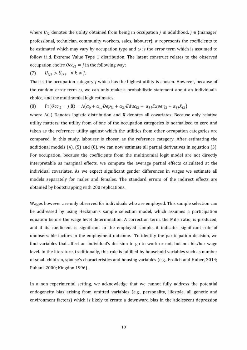
where 𝑈𝑗2 denotes the utility obtained from being in occupation 𝑗 in adulthood, 𝑗 ∈ {manager,

professional, technician, community workers, sales, labourer}, 𝛼 represents the coefficients to

be estimated which may vary by occupation type and 𝜔 is the error term which is assumed to

follow i.i.d. Extreme Value Type 1 distribution. The latent construct relates to the observed

occupation choice 𝑂𝑐𝑐𝑖2 = 𝑗 in the following way:

(7) 𝑈𝑖𝑗2 > 𝑈𝑖𝑘2 ∀ 𝑘 ≠ 𝑗.

That is, the occupation category 𝑗 which has the highest utility is chosen. However, because of

the random error term 𝜔, we can only make a probabilistic statement about an individual’s

choice, and the multinomial logit estimates:

(8) Pr (𝑂𝑐𝑐𝑖2 = 𝑗|Χ) = Λ(𝛼0 + 𝛼1𝑗𝐷𝑒𝑝𝑖1 + 𝛼2𝑗𝐸𝑑𝑢𝑐𝑖2 + 𝛼3𝑗𝐸𝑥𝑝𝑒𝑟𝑖2 + 𝛼4𝑗𝑋𝑖2)

where Λ(. ) Denotes logistic distribution and X denotes all covariates. Because only relative

utility matters, the utility from of one of the occupation categories is normalised to zero and

taken as the reference utility against which the utilities from other occupation categories are

compared. In this study, labourer is chosen as the reference category. After estimating the

additional models (4), (5) and (8), we can now estimate all partial derivatives in equation (3).

For occupation, because the coefficients from the multinomial logit model are not directly

interpretable as marginal effects, we compute the average partial effects calculated at the

individual covariates. As we expect significant gender differences in wages we estimate all

models separately for males and females. The standard errors of the indirect effects are

obtained by bootstrapping with 200 replications.

Wages however are only observed for individuals who are employed. This sample selection can

be addressed by using Heckman’s sample selection model, which assumes a participation

equation before the wage level determination. A correction term, the Mills ratio, is produced,

and if its coefficient is significant in the employed sample, it indicates significant role of

unobservable factors in the employment outcome. To identify the participation decision, we

find variables that affect an individual’s decision to go to work or not, but not his/her wage

level. In the literature, traditionally, this role is fulfilled by household variables such as number

of small children, spouse’s characteristics and housing variables (e.g., Frolich and Huber, 2014;

Puhani, 2000; Kingdon 1996).

In a non-experimental setting, we acknowledge that we cannot fully address the potential

endogeneity bias arising from omitted variables (e.g., personality, lifestyle, all genetic and

environment factors) which is likely to create a downward bias in the adolescent depression

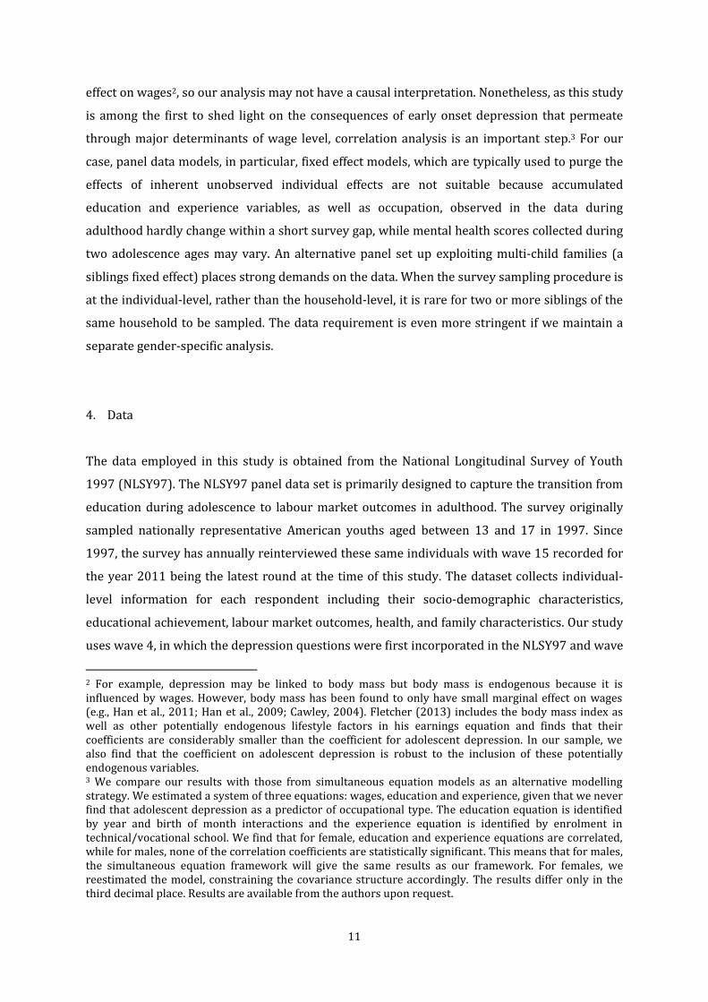
11

effect on wages2, so our analysis may not have a causal interpretation. Nonetheless, as this study

is among the first to shed light on the consequences of early onset depression that permeate

through major determinants of wage level, correlation analysis is an important step.3 For our

case, panel data models, in particular, fixed effect models, which are typically used to purge the

effects of inherent unobserved individual effects are not suitable because accumulated

education and experience variables, as well as occupation, observed in the data during

adulthood hardly change within a short survey gap, while mental health scores collected during

two adolescence ages may vary. An alternative panel set up exploiting multi-child families (a

siblings fixed effect) places strong demands on the data. When the survey sampling procedure is

at the individual-level, rather than the household-level, it is rare for two or more siblings of the

same household to be sampled. The data requirement is even more stringent if we maintain a

separate gender-specific analysis.

4. Data

The data employed in this study is obtained from the National Longitudinal Survey of Youth

1997 (NLSY97). The NLSY97 panel data set is primarily designed to capture the transition from

education during adolescence to labour market outcomes in adulthood. The survey originally

sampled nationally representative American youths aged between 13 and 17 in 1997. Since

1997, the survey has annually reinterviewed these same individuals with wave 15 recorded for

the year 2011 being the latest round at the time of this study. The dataset collects individual-

level information for each respondent including their socio-demographic characteristics,

educational achievement, labour market outcomes, health, and family characteristics. Our study

uses wave 4, in which the depression questions were first incorporated in the NLSY97 and wave

2 For example, depression may be linked to body mass but body mass is endogenous because it is influenced by wages. However, body mass has been found to only have small marginal effect on wages (e.g., Han et al., 2011; Han et al., 2009; Cawley, 2004). Fletcher (2013) includes the body mass index as well as other potentially endogenous lifestyle factors in his earnings equation and finds that their coefficients are considerably smaller than the coefficient for adolescent depression. In our sample, we also find that the coefficient on adolescent depression is robust to the inclusion of these potentially endogenous variables. 3 We compare our results with those from simultaneous equation models as an alternative modelling strategy. We estimated a system of three equations: wages, education and experience, given that we never find that adolescent depression as a predictor of occupational type. The education equation is identified by year and birth of month interactions and the experience equation is identified by enrolment in technical/vocational school. We find that for female, education and experience equations are correlated, while for males, none of the correlation coefficients are statistically significant. This means that for males, the simultaneous equation framework will give the same results as our framework. For females, we reestimated the model, constraining the covariance structure accordingly. The results differ only in the third decimal place. Results are available from the authors upon request.

12

6, which is the next available depression data. At these two waves, our respondents are in their

adolescent years. We analyse their employment outcomes 9-10 years later in wave 14 and wave

15. We pooled the two waves together, giving a total sample size of 11,014 (6,298 unique

respondents), after excluding those who are still completing their education (13% of the

original sample) and individuals with missing information (9% of the remaining original

sample).

The depression status information is obtained from the 5-item Mental Health Inventory (MHI-5)

provided within dataset. The MHI-5 score comprises of five multiple choice questions relating to

depressive and anxiety symptoms. Of the five questions, two are specific to depression: “how

often have you felt down in the last month?” and “how often have you felt depressed in the last

month?” The other questions are about calmness, happiness and anxiety. We define individuals

who answered “all the time” or “most of the time” to any of the two depression questions as

depressed. We believe that this measure is more accurate than using the average score from all

five questions in the MHI-5 which is commonly done in the literature. For instance, we find that

the correlation between the average score and the specific depression question is not very high

(around 0.5).

The wage used in this study is measured as rate of hourly pay received from the primary full

time job. We define the primary job as the job which the individual works the most in terms of

hours per week if he or she holds more than one job. If an individual works the same amount of

hours for multiple jobs, we define the main job as the job that has the earliest start date. The

hourly wage rate is computed for all types of jobs by NLSY97; if respondents are not being paid

by the hour, the hourly wage is computed from regular earnings and regular hours (i.e.,

excluding tips, bonuses, commissions, overtime, etc). Education is measured as the total number

of years of formal education completed. Later we also use binary indicators for high school

completion and post-school certificates (having a degree higher than a high school diploma).

The aim of using these binary indicators is to allow for possible non-linearity in the depression

effect on education, for example, it is possible that adolescent depression impairs education

primarily by discouraging individuals to pursue higher studies. Adult work experience is

accumulated experience to date. For occupational outcomes, we categorise individuals as

working in one of six groups. To group the individuals according to job type we use the 2002 U.S

Census Bureau classification codes attached to each job in NLSY97. In total, there were 509

unique codes each corresponding to a different job title. A worker belongs to one of the

following groups: managers, professionals, technicians, community or hospitality workers, sales

13

or administrative workers, and labourers or machinery workers. Managers are those working in

roles such as chief executives, financial managers, natural sciences manager and legislators.

Professionals include physicians, accountants, lawyers and engineers. Carpenters, electricians

and maintenance workers are technicians, while individuals working in hospitality and service

type roles such as nurses, fire fighters and bartenders are classified as community or hospitality

workers. Sales or administration include salespersons, cashiers and sales agents, while janitors,

machine operators and construction helpers are grouped as labourers or machinery workers.

For control variables, we include age at the interview date, race, marital status, region of

residence and residence in a rural area. We also control for mother’s and father’s education as

an indirect proxy for socioeconomic status during upbringing, aspiration in the family and

inheritance of skills. This may capture some of the effects of genetic factors on education and

labour market outcomes, to the extent that these genetic factors are inheritable from parents.

There is also a well-established literature finding that children and adolescents in lower income

families have higher prevalence of mental and physical health problems (e.g., Geoffard and

Apouey, 2013; Reinhold and Jurges, 2012; Yoshikawa et al., 2012), and they are more likely to

earn less as adults than those from more privileged families (e.g., Haas et al., 2011; Smith, 2009).

Thus controlling for family socio-economic status (SES) is important. In the wage equation we

also control for wage differentials arising from part time status, self-employed status and having

undertaken vocational training.

To account for sample selection of observed wages, we estimate Heckman sample selection

model. The participation equation may be seen as a reduced form specification, where labour

market opportunities are reflected by demographics and parental education. The exclusion

restriction for the participation decision is given by the presence of children under 6 years of

age. We have also considered spouse’s working status, household size and coresidence status

with parents but they fail the exclusion restriction test (i.e., they also influence wage level).

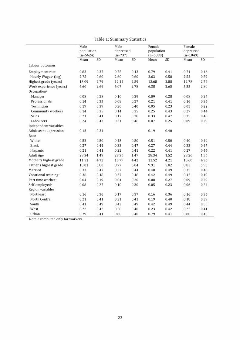
Table 1 presents the summary statistics overall and for those who experienced adolescent

depression. The adolescent depression rates are 13% and 19% for males and females,

respectively. Males have higher employment rates, average hourly wages, fewer years of

education and more years of experience than females. We also observe a significant labour

market gap by depression status. The average wage for males who experienced depression

during adolescence is similar to males who did not experience adolescent depression, whilst

females who experienced adolescent depression have a much lower average wage than those

14

who did not (almost $3). Both the stock of education and experience are generally lower for

those who experienced adolescent depression. Males are predominantly employed as

technicians, sales workers and labourers whilst the majority of females are professionals,

community workers or sales workers. Those who experienced adolescent depression are much

less likely to hold a job as professionals. Professional workers had the highest average wage

compared with workers in other categories. Approximately half of the sample is non-Black or

non-Hispanic, the average adult age is 28 and about 80% lived in urban areas. The table also

shows positive correlation between adolescence mental wellness and parental education.

[Table 1 here]

5. Results

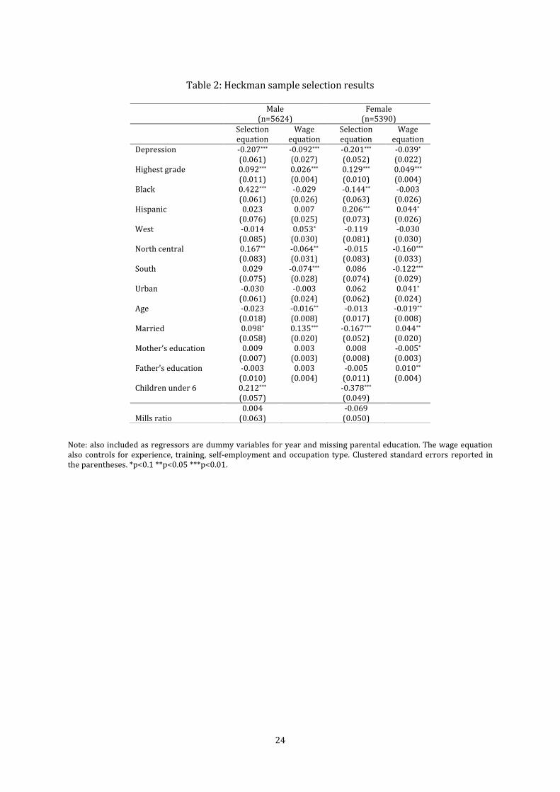
We first present the results for the sample selection model in Table 2. In the participation

equation (column [1]), adolescent depression has a negative impact on participation for both

males and females. The presence of young children increases the propensity to work for males

whilst reduces female labour force participation. In no case do we find the Mills ratio significant,

indicating that we can estimate the wage equation on the workers sample. From here on, we

focus on results from the workers sample.

[Table 2 here]

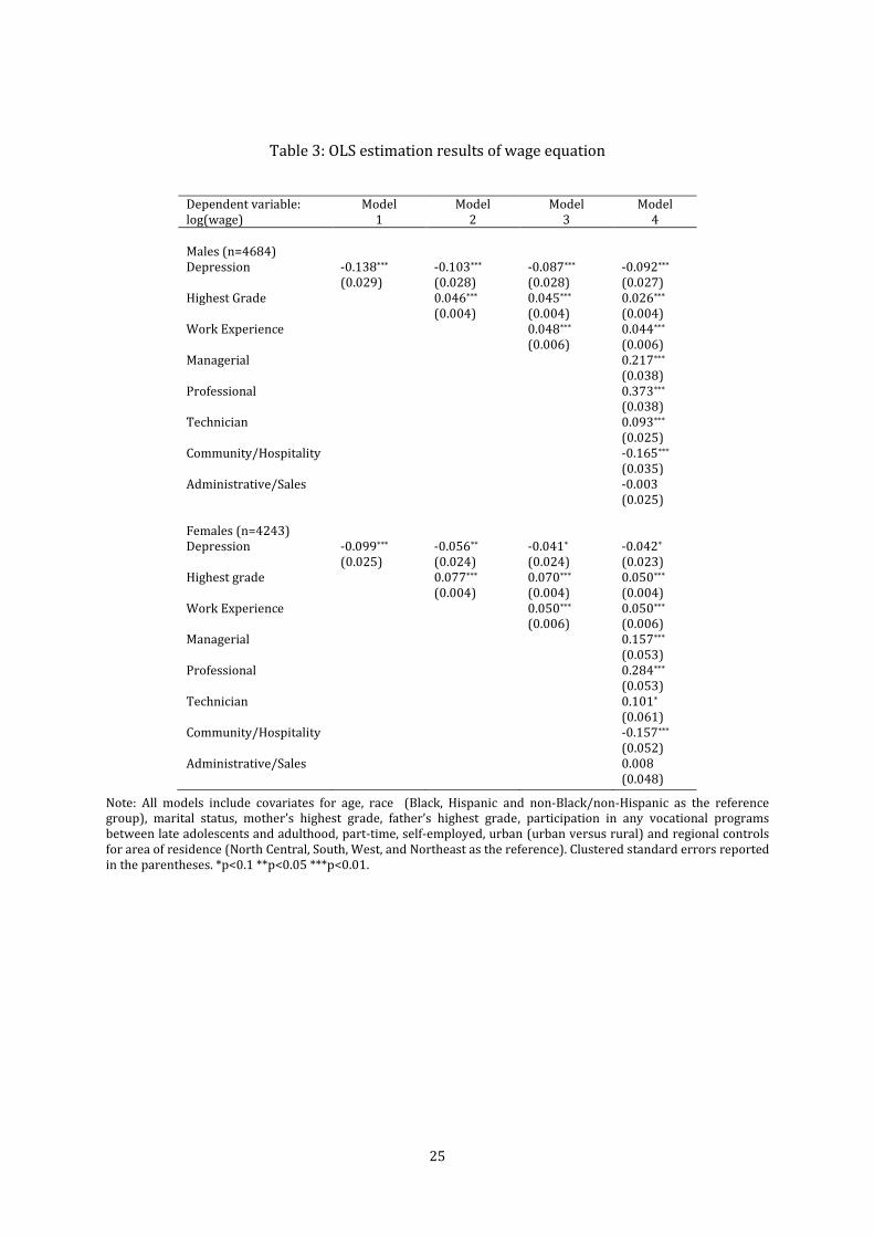
Table 3 reports the results from four wage equation specifications, starting with the first model

without any of the potential pathway variables. The subsequent models progressively add the

pathway variables to the base model, starting with education, work experience and then

occupational type.

[Table 3 here]

Across all specifications we find that depression during adolescence has a persistent significant

negative impact on adult wages. Starting with the baseline results in Model 1, the direct hourly

wage penalty associated with adolescent depression is 13.8% for males and 9.9% females,

respectively. Adding education and experience, the direct effect of adolescent depression on

wages is reduced suggesting a negative correlation with education and experience. The change

in the direct effect is more dramatic for females. In the full specification in Model 4, the direct

15

wage penalty associated with adolescent depression is 9.2% for males and 4.2% for females.

This finding of significant direct effect has important policy implication in terms of mental

health promotion among young individuals. While it is difficult to completely ascertain what

drives the direct effect, the sociology literature on personality traits offers one possible

interpretation. It may be that individuals who experienced depression as adolescence enter the

labour market with certain negative traits or personality characteristics that may impede their

integration into the workplace and lower their opportunities for a promotion or involvements

in high-yielding projects which in turn mean lower wages. Our estimates are lower than

Fletcher’s (2013) estimate of about 15% on earnings, which comprise of both wage and work

hours, suggesting that adolescent depression also impacts work hours negatively.

As expected, education is positively associated with wage rates, and we find that the return to

education is much higher for females. An additional year of education is associated to a 5.0%

increase in hourly wages for females, as opposed to only 2.6% for males.4 On the other hand, the

returns for an additional year of work experience are comparable for males and females, 4.4%

and 5.0% for males and females, respectively. Professionals are the highest paid job group

followed by managers, whilst community workers are the lowest paid job group. Male

professionals and managers earn 53.8% and 38.2% higher hourly wages, respectively, than

male community workers. For females, this wage gap is 44.1% and 31.4%.

A comparison of the adolescent depression coefficients in Models 2-3 with that in Model 1

confirms education and work experience as strong mediators of the adolescent depression

impact on wages. As is the case with occupational type, the adolescent depression coefficient

reduces further in Model 4 suggesting that females who suffered from adolescent depression

tend to end up in lower paying jobs. Turning to the control variables, we find no significant

wage differentials by race and parental education for males. For females, Hispanics earn higher

hourly wages than Whites while paternal education also positively impacts their hourly wages.

In terms of the geographical variations in wages, we find that workers in the South and North

Central earn less than those in the North East.5

4 Using the Panel Study of Income Dynamics (PSID) 2009 data, for a sample with comparable average age, education and wage levels, we estimated that the return to education is also around 3% for males and 2% for females. Dougherty (2005) also find a return of 5% for males and 3% for females in their NLSY samples from 1988-2000. Compared with estimates from older data sets, such as Angrist and Krueger’s (1991) samples in 1970-1980s which gives an estimate of 8%, these estimates are lower. 5 Full results are available from authors.

16

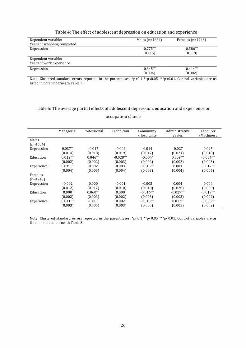
Table 4 presents the marginal effect of adolescent depression on education and experience

obtained by OLS. It indicates that the experience of depression before adulthood is associated

with a significant reduction in educational outcomes for both genders. Females who experience

adolescent depression have 0.59 years less stock of education compared to their counterparts

who did not experience adolescent depression. The education penalty for males is larger at 0.78

years. Accumulated education is significantly positively correlated with parental education,

especially father’s education; the strength of the correlation coefficient of father’s education is

three to four times greater than that of mother’s education.

[Table 4 here]

Adolescent depression is also negatively associated with total work experience for both males

and females. Females who were depressed as adolescents have 0.41 years less total adult work

experience than their non-depressed counterparts, or approximately 6.2% less years of total

work experience compared to the female sample average. For males, adolescent depression is

associated with 0.35 years less total adult work experience than their non-depressed

counterparts, or approximately 5.2% less years of total work experience compared to the male

sample average.

Table 5 reports the average partial effects from multinomial logit model. For each gender, we

find that adolescent depression has no effect on occupational sorting, except for managerial

occupations for males. All else equal, males who experienced depression during adolescence are

more likely to work in managerial jobs than labourers. Because the NLSY97 does not distinguish

between employees and self-employed individuals when applying the census job classification

codes, this result may capture the higher likelihood of males who were depressed during

adolescence to be the manager of their own business. For instance, when we interacted the

depression with self-employment variable, significant positive coefficients are only found when

the self-employment dummy variable is switched on. Since managerial wage is the second

highest among the six occupation groups, this positive relationship explains the increase in the

size of the direct effect of adolescent depression on wage for males when occupation choice is

included in the model (Models 3 and 4 in Table 3). Education has the greatest effect on

increasing the probability of being employed in professional occupations for both genders. An

additional year of education increases the probability of working in professional jobs by 4.6 and

6.0 percentage points for men and women, respectively. Education also increases the

probability of males being employed in managerial jobs. On the other hand, education lowers

the probability of working as labourers. Total work experience has significant positive effects on

17

the likelihood of being employed in managerial jobs. An additional year of work experience is

associated with higher probability of being employed in managerial jobs by 1.9 and 1.1

percentage points for males and females, respectively. In contrast, those with more work

experience are less likely to work in the lowest paying job groups, community/ hospitality jobs.

[Table 5 here]

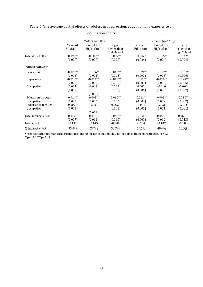
In Table 6 we use all of these results to calculate the total effect of adolescent depression. The

‘Years of Education’ columns correspond to the result in Table 4, where education is measured

using a continuous variable for years of education. The results for those who ‘completed high

school’ and those who hold a degree higher than high school are based on binary indicators for

high school diploma versus no high school diploma and having a post-school degree versus not

having a post-school degree, respectively, rather than a continuous variable. They aim to shed

light on the location of the depression effect. Overall, we find that, the total effect of adolescent

depression is higher for males than for females, between 10–15%. However the mechanisms

behind this total effect are very different for males and females. For males, the total effect is

primarily driven by the direct effect: about 66%, or 64% if we do not count the occupation

channel which is statistically insignificant. On the other hand, for females, the indirect effects

are larger. The indirect effects operate through both lower education and experience, which are

both also responsible for sorting into lower paying jobs. Depression lowers the probability of

graduating from high school and it also discourages them from undertaking higher studies. This

in turn leads to lower paying jobs. For males, the lower educational attainment contributes to a

further reduction in wages by 2.0%, or 14% of the total effect, while for females, this figure is

2.9%, or 28% of the total effect. Lower experience makes up 11% of the total effect for males

and 20% for females. The indirect effect of adolescent depression operating through education

on occupational type amounts to about 10% of the total effect for both genders via this pathway.

This is largely due to the reduced likelihood of being employed as professionals (which is the

highest paying occupation) due to the loss of education.

[Table 6 here]

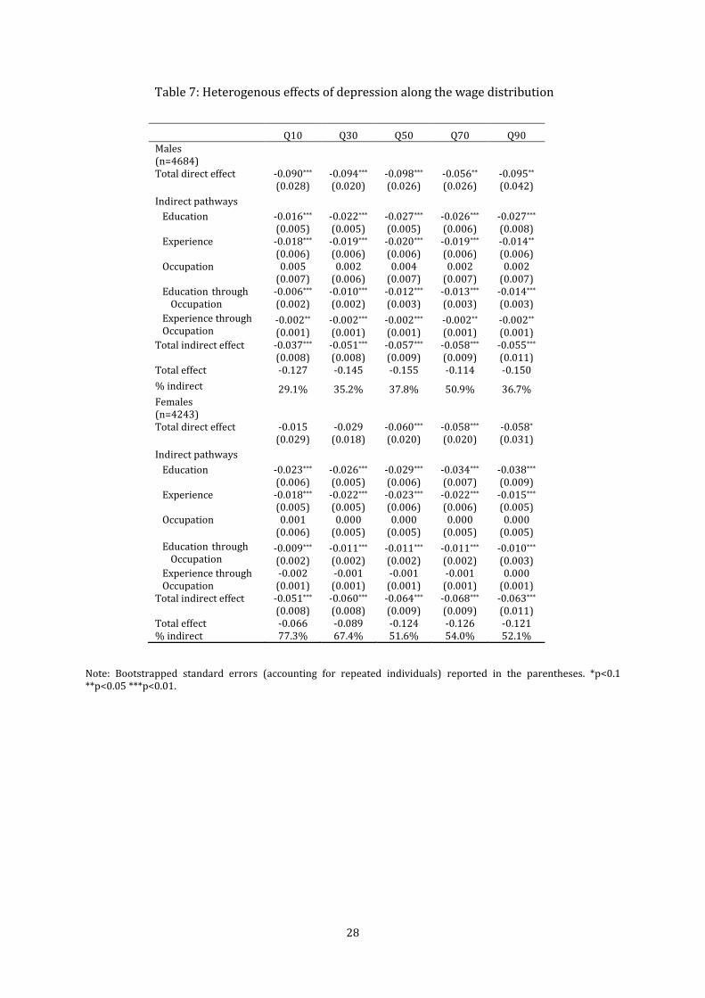
In Table 7, we explore heterogenous effects along the wage distribution. We estimate the wage

equation by quantile regressions to allow varying strength of relationships between wages,

adolescent depression, education, experience and education across wage levels. For each

gender, there is significant heterogeneity in the direct effect, at least between the bottom and

18

top quintiles. For males, the total effect of adolescent depression has a narrow range, around

11-15%, whilst for females the range is wider, between 7 to 13%. For males, the indirect effect

as a share of the total effect tends to be smaller than the indirect effect. In contrast, for females,

the indirect effect is almost always dominant, especially at low wages. This changing pattern of

the direct versus indirect effects reflects the larger role of education at high wage levels, and

also the importance of favourable personal traits at different wage levels. Especially for female

workers, personality is very important to maintain a top-wage job.

[Table 7 here]

6. Conclusion

Unlike most studies in the mental health literature which link current outcomes with current

mental health status, we examine the impact of mental illness, specifically, depression that

occurred when the now adult individuals were still in adolescence. We focus on the labour

market achievement of employed individuals, as measured by their hourly wage rate in the

early career stage (age 25-31). We find that adolescent depression has a direct, independent

impact on adult wages, lowering male workers’ wage by 9% and female workers’ wage by 4%.

In addition, adolescent depression disrupts the accumulation of human capital which translates

to lower wages. The total effect of adolescent depression on adult wages is estimated to be

around 10-15% on average. This result highlights the significant role of human capital

accumulation as a pathway which induces the wage penalty, especially for females. Almost half

of the total wage penalty for females is indirect due to the reductions of education stock,

especially attainment of post high school qualification, and accumulated work experience due to

adolescent depression. For males, the indirect effect due to loss of education and experience

accounted for about a quarter of the total wage penalty. The education effect also filters through

occupation sorting as we find the lower accumulated education associated with adolescent

depression reduces the probability of being employed in high paying jobs, particularly

professionals. As we find large indirect effects operating through education, a policy implication

is to intervene to assist depressed students continuing at school and into higher education. This

may be achieved through support group or assistance programs implemented in schools and

colleges. A number of studies have reported positive effects of school-based mental health

promotion efforts on significantly reducing students’ anxiety, behavior problems and depressive

symptoms, as well as increasing their communication skills and self-confidence (Durlak and

Wells, 1997; Durlack et al., 2011). Moreover, such programs may be particularly effective for

19

girls. For instance, Lynch et al (2014) find a significant link between behavioral problems and

high school graduation among girls, but not among boys. Girls may also be more likely to

participate in intervention program than boys (Wang and Eccles, 2004).

20

References

Adler, D., McLaughlin, T., Rogers, W., et al. (2006). Job performance deficits due to depression.

American Journal of Psychiatry, 163(9), 1569-1576.

Angrist, JD, Krueger, AB. (1991). Does Compulsory School Attendance Affect Schooling and

Earnings? The Quarterly Journal of Economics, 106(4), 979-1014.

Asarnow, J. R., Jaycox, L. H., Duan, N., et al. (2005). Depression and role impairment among

adolescents in primary care clinics. Journal of Adolescent Health, 37, 477–483.

Beck, A., Crain, A. L., Solberg, L. I., et al. (2011). Severity of depression and magnitude of

productivity loss. The Annals of Family Medicine, 9(4), 305-311.

Berndt, E. R., Koran, L. M., Finkelstein, S. N., et al. (2000). Lost human capital from early-onset

chronic depression. American Journal of Psychiatry, 157(6), 940-947.

Currie, J., Stabile, M. (2006). Child mental health and human capital accumulation: The case of

ADHD. Journal of Health Economics, 25(6), 1094-1118.

Currie, J., Stabile, M. (2007). Mental health in childhood and human capital. NBER Working

Paper No.13217. NBER, Cambridge, MA.

Cawley, J. (2004). The impact of obesity on wages. Journal of Human Resources, 39(2), 451-474.

Ding, W., Lehrer, S., Rosenquist, N., Audrain-McGovern, J. 2006. The impact of poor health on

education: new evidence using genetic markers. NBER Working Paper 12304.

Dougherty, C. (2005). Why are the returns to schooling higher for women than for men?. Journal

of Human Resources, 40(4), 969-988.

Durlak, J.A., Wells, A.M. (1997). Primary prevention mental health programs for children and

adolescents: A meta-analytic review. American journal of community psychology, 25(2),

115-152.

Durlak, J.A., Weissberg, R.P., Dymnicki, A.B. et al. (2011). The impact of enhancing students’

social and emotional learning: A meta‐analysis of school‐based universal interventions.

Child development, 82(1), 405-432.

Ferrari, A.J., Charlson, F.J., Norman, R.E. et al. Burden of depressive disorders by country, sex,

age, and year: Findings from the global burden of disease study 2010. PLOS Medicine 10,

no 11.

Fergusson, D. M., Boden, J. M., & Horwood, L. J. (2007). Recurrence of major depression in

adolescence and early adulthood, and later mental health, educational and economic

outcomes. The British Journal of Psychiatry, 191(4), 335-342.

Fletcher, J. (2013). Adolescent Depression and Adult Labor Market Outcomes. Southern

Economic Journal, 80(1), 26-49.

21

Fletcher, J. (2010). Adolescent depression and educational attainment: results using sibling

fixed effects. Health Economics, 19(7), 855-871.

Fombonne, E., Wostear, G., Cooper, V., et al. (2001). The Maudsley long-term follow-up of child

and adolescent depression: Psychiatric outcomes in adulthood. The British Journal of

Psychiatry, 179(3), 210-217.

Fritjers, P., Johnston, D., Shields, M. (2010). Mental Health and Labour Market Participation:

Evidence from IV Panel Data Models. IZA Discussion Paper No 4883.

Frolich, M, Huber, M. (2014). Direct and Indirect Treatment Effects: Causal Chains and

Mediation Analysis with Instrumental Variables. IZA Working Paper No. 8280.

Geoffard, P.Y., Apouey, B. (2013). Family income and child health in the UK. Journal of health

economics, 32(4), 715-727.

Greenberg, P. E., Kessler, R. C., Birnbaum, H. G., et al. (2003). The economic burden of depression

in the United States: How did it change between 1990 and 2000? Journal of Clinical

Psychiatry, 64, 1465-1475.

Haas, S.A., Glymour, M.M., Berkman, L.F. (2011). Childhood health and labor market inequality

over the life course. Journal of health and social behavior, 52(3), 298-313.

Han, E., Norton, E. C., & Powell, L. M. (2011). Direct and indirect effects of body weight on adult

wages. Economics & Human Biology, 9(4), 381-392.

Han, E., Norton, E. C., & Stearns, S. C. (2009). Weight and wages: fat versus lean paychecks.

Health Economics, 18(5), 535-548.

Jokela, M., & Keltikangas-Järvinen, L. (2011). The association between low socioeconomic status

and depressive symptoms depends on temperament and personality traits. Personality

and Individual Differences, 51(3), 302-308.

Jylha, P., Melartin, T., Rytsala, H. & Isometsä, E. (2009). Neuroticism, introversion, and major

depressive disorder—traits, states, or scars. Depression and Anxiety, 26, 325–334.

Kaplan, E. (2011). Three Essays on Labor Economics. Mimeo, University of California, Santa

Barbara. Available from: http://gradworks.umi.com/34/95/3495683.html

Karsten, J., Penninx, B. W., Riese, H., et al. (2012). The state effect of depressive and anxiety

disorders on big five personality traits. Journal of psychiatric research, 46(5), 644-650.

Kingdon, G. (1996). The quality and efficiency of private and public education: a case‐study of

urban India. Oxford Bulletin of Economics and Statistics, 58(1), 57-82.

Lundborg, P., Nilsson, A., Rooth, D. (2014). Adolescent health and adult labor market outcomes.

Journal of Health Economics 37, 25-40.

22

Lynch, R.J., Kistner, J.A., Allan, N.P. (2014). Distinguishing among disruptive behaviors to help

predict high school graduation: Does gender matter? Journal of School Psychology

forthcoming.

Mueller, G., & Plug, E. (2006). Estimating the effect of personality on male and female earnings.

Industrial and Labor Relations Review, 3-22.

Murray, M.P. (2006). Avoiding invalid instruments and coping with weak instruments. The

journal of economic perspectives, 20(4), 111-132.

Murray C.J.L. & Lopez, A.D. 1996, The global burden of disease: a comprehensive assessment of

mortality and disability from diseases, injuries and risk factors in 1990 and projected to

2020, (Global Burden of disease and Injury Series), Harvard University Press, Cambridge.

Piccinelli, M., & Wilkinson, G. (2000). Gender differences in depression Critical review. The

British Journal of Psychiatry, 177(6), 486-492.

Puhani, P. (2000). The Heckman correction for sample selection and its critique. Journal of

economic surveys, 14(1), 53-68.

Quiroga, C. V., Janosz, M., Bisset, S., & Morin, A. J. (2013). Early adolescent depression symptoms

and school dropout: Mediating processes involving self-reported academic competence

and achievement. Journal of Educational Psychology, 105(2), 552.

Reinhold, S., Jürges, H. (2012). Parental income and child health in Germany. Health Economics,

21(5), 562-579.

Roeser, R., Eccles, J., Strobel, K. (1998). Linking the study of schooling and mental health:

selected issues and empirical illustrations at the level of the individual. Educational

Psychologist, 33(4), 153–176.

Sands, E. (2008). Linking Depressed Earnings to Adolescent Depression. Undergraduate

Economic Review, 4(1), 10.

Smith, J. (2009). The impact of childhood health on adult labor market outcomes. The review of

economics and statistics, 91(3), 478-489.

Wang, P. S., Beck, A. L., Berglund, P. et al. (2004). Effects of major depression on moment-in-time

work performance. American Journal of Psychiatry, 161, 1885–1891.

Wang, M.T., Eccles, J.S. (2012). Social support matters: Longitudinal effects of social support on

three dimensions of school engagement from middle to high school. Child development,

83(3), 877-895.

Yoshikawa, H., Aber, J.L., Beardslee, W.R. (2012). The effects of poverty on the mental,

emotional, and behavioral health of children and youth: implications for prevention.

American Psychologist, 67(4), 272.

23

Table 1: Summary Statistics

Male population (n=5624)

Male depressed (n=737)

Female population (n=5390)

Female depressed (n=1049)

Mean SD Mean SD Mean SD Mean SD

Labour outcomes

Employment rate 0.83 0.37 0.75 0.43 0.79 0.41 0.71 0.46

Hourly Wagesa (log) 2.75 0.60 2.60 0.60 2.63 0.58 2.52 0.59

Highest grade (years) 13.09 2.79 12.12 2.59 13.68 2.88 12.78 2.74

Work experience (years) 6.60 2.69 6.07 2.78 6.38 2.65 5.55 2.80

Occupationa

Manager 0.08 0.28 0.10 0.29 0.09 0.28 0.08 0.26

Professionals 0.14 0.35 0.08 0.27 0.21 0.41 0.16 0.36

Technician 0.19 0.39 0.20 0.40 0.05 0.23 0.05 0.22

Community workers 0.14 0.35 0.14 0.35 0.25 0.43 0.27 0.44

Sales 0.21 0.41 0.17 0.38 0.33 0.47 0.35 0.48

Labourers 0.24 0.43 0.31 0.46 0.07 0.25 0.09 0.29

Independent variables

Adolescent depression 0.13 0.34 0.19 0.40

Race

White 0.52 0.50 0.45 0.50 0.51 0.50 0.40 0.49

Black 0.27 0.44 0.33 0.47 0.27 0.44 0.33 0.47

Hispanic 0.21 0.41 0.22 0.41 0.22 0.41 0.27 0.44

Adult Age 28.34 1.49 28.36 1.47 28.34 1.52 28.26 1.56

Mother’s highest grade 11.51 4.32 10.79 4.42 11.52 4.21 10.60 4.36

Father’s highest grade 10.01 5.80 8.77 6.04 9.91 5.82 8.83 5.90

Married 0.33 0.47 0.27 0.44 0.40 0.49 0.35 0.48

Vocational traininga 0.36 0.48 0.37 0.48 0.42 0.49 0.42 0.49

Part time workera 0.04 0.19 0.04 0.20 0.08 0.27 0.09 0.29

Self-employeda 0.08 0.27 0.10 0.30 0.05 0.23 0.06 0.24

Region variables

Northeast 0.16 0.36 0.17 0.37 0.16 0.36 0.16 0.36

North Central 0.21 0.41 0.21 0.41 0.19 0.40 0.18 0.39

South 0.41 0.49 0.42 0.49 0.42 0.49 0.44 0.50

West 0.22 0.42 0.20 0.40 0.23 0.42 0.22 0.41

Urban 0.79 0.41 0.80 0.40 0.79 0.41 0.80 0.40

Note: a computed only for workers.

24

Table 2: Heckman sample selection results

Note: also included as regressors are dummy variables for year and missing parental education. The wage equation also controls for experience, training, self-employment and occupation type. Clustered standard errors reported in the parentheses. *p<0.1 **p<0.05 ***p<0.01.

Male

(n=5624) Female

(n=5390)

Selection equation

Wage equation

Selection equation

Wage equation

Depression

-0.207***

(0.061) -0.092***

(0.027) -0.201***

(0.052) -0.039*

(0.022) Highest grade

0.092***

(0.011) 0.026***

(0.004) 0.129***

(0.010) 0.049***

(0.004) Black

0.422***

(0.061) -0.029

(0.026) -0.144**

(0.063) -0.003

(0.026) Hispanic

0.023 (0.076)

0.007 (0.025)

0.206***

(0.073) 0.044*

(0.026) West

-0.014 (0.085)

0.053*

(0.030) -0.119 (0.081)

-0.030 (0.030)

North central

0.167**

(0.083) -0.064** (0.031)

-0.015 (0.083)

-0.160***

(0.033) South

0.029 (0.075)

-0.074*** (0.028)

0.086 (0.074)

-0.122***

(0.029) Urban

-0.030 (0.061)

-0.003 (0.024)

0.062 (0.062)

0.041* (0.024)

Age

-0.023 (0.018)

-0.016** (0.008)

-0.013 (0.017)

-0.019**

(0.008) Married

0.098*

(0.058) 0.135*** (0.020)

-0.167***

(0.052) 0.044**

(0.020) Mother’s education

0.009 (0.007)

0.003 (0.003)

0.008 (0.008)

-0.005*

(0.003) Father's education

-0.003 (0.010)

0.003 (0.004)

-0.005 (0.011)

0.010**

(0.004) Children under 6

0.212***

(0.057)

-0.378*** (0.049)

Mills ratio

0.004 (0.063)

-0.069 (0.050)

25

Table 3: OLS estimation results of wage equation

Note: All models include covariates for age, race (Black, Hispanic and non-Black/non-Hispanic as the reference group), marital status, mother’s highest grade, father’s highest grade, participation in any vocational programs between late adolescents and adulthood, part-time, self-employed, urban (urban versus rural) and regional controls for area of residence (North Central, South, West, and Northeast as the reference). Clustered standard errors reported in the parentheses. *p<0.1 **p<0.05 ***p<0.01.

Dependent variable: log(wage)

Model 1

Model 2

Model 3

Model 4

Males (n=4684)

Depression -0.138***

(0.029) -0.103***

(0.028) -0.087***

(0.028) -0.092***

(0.027) Highest Grade 0.046***

(0.004) 0.045***

(0.004) 0.026***

(0.004) Work Experience 0.048***

(0.006) 0.044***

(0.006) Managerial

0.217***

(0.038) Professional 0.373***

(0.038) Technician

0.093***

(0.025) Community/Hospitality

-0.165***

(0.035) Administrative/Sales -0.003

(0.025) Females (n=4243)

Depression -0.099***

(0.025) -0.056**

(0.024) -0.041*

(0.024) -0.042* (0.023)

Highest grade 0.077***

(0.004) 0.070***

(0.004) 0.050***

(0.004) Work Experience 0.050***

(0.006) 0.050***

(0.006) Managerial

0.157*** (0.053)

Professional 0.284***

(0.053) Technician

0.101*

(0.061) Community/Hospitality

-0.157***

(0.052) Administrative/Sales 0.008

(0.048)

26

Table 4: The effect of adolescent depression on education and experience

Dependent variable: Years of schooling completed

Males (n=4684) Females (n=4243)

Depression -0.775***

(0.115) -0.586***

(0.118)

Dependent variable: Years of work experience

Depression -0.345***

(0.094) -0.414*** (0.082)

Note: Clustered standard errors reported in the parentheses. *p<0.1 **p<0.05 ***p<0.01. Control variables are as listed in note underneath Table 3.

Table 5: The average partial effects of adolescent depression, education and experience on

occupation choice

Note: Clustered standard errors reported in the parentheses. *p<0.1 **p<0.05 ***p<0.01. Control variables are as listed in note underneath Table 3.

Managerial Professional Technician Community /Hospitality

Administrative /Sales

Labourer /Machinery

Males (n=4684)

Depression 0.037** (0.014)

-0.017 (0.018)

-0.004 (0.019)

-0.014 (0.017)

-0.027 (0.021)

0.025 (0.018)

Education 0.012*** (0.002)

0.046*** (0.002)

-0.028*** (0.003)

-0.004* (0.002)

0.009*** (0.003)

-0.034*** (0.003)

Experience

0.019*** (0.004)

0.002 (0.003)

0.003 (0.004)

-0.013*** (0.003)

0.001 (0.004)

-0.012*** (0.004)

Females (n=4243)

Depression -0.002 (0.012)

0.000 (0.017)

-0.001 (0.010)

-0.005 (0.018)

0.004 (0.020)

0.004 (0.009)

Education 0.000 (0.002)

0.060*** (0.003)

0.000 (0.002)

-0.016*** (0.003)

-0.027*** (0.003)

-0.017*** (0.002)

Experience 0.011*** (0.003)

-0.003 (0.005)

0.002 (0.003)

-0.015*** (0.005)

0.012** (0.005)

-0.006***

(0.002)

27

Table 6: The average partial effects of adolescent depression, education and experience on

occupation choice

Note: Bootstrapped standard errors (accounting for repeated individuals) reported in the parentheses. *p<0.1 **p<0.05 ***p<0.01.

Males (n=4684) Females (n=4243)

Years of Education

Completed High school

Degree higher than High School

Years of Education

Completed High school

Degree higher than High School

Total direct effect -0.092***

(0.028) -0.102***

(0.028) -0.097***

(0.028) -0.042*

(0.024) -0.055**

(0.024) -0.042*

(0.024)

Indirect pathways

Education -0.020***

(0.004) -0.006**

(0.002) -0.016***

(0.004) -0.029***

(0.007) -0.007**

(0.003) -0.028***

(0.006) Experience -0.015***

(0.005) -0.014***

(0.005) -0.016***

(0.005) -0.021***

(0.005) -0.024***

(0.005) -0.023***

(0.005) Occupation 0.004

(0.007) -0.014*

(0.008)

0.001 (0.007)

0.000 (0.006)

-0.010

(0.009) -0.000

(0.007)

Education through Occupation

-0.014***

(0.003) -0.008***

(0.002) -0.010***

(0.002) -0.011***

(0.003) -0.008***

(0.002) -0.010***

(0.002) Experience through Occupation

-0.002***

(0.001) -0.001

(0.001)

-0.002**

(0.001) -0.001

(0.001) -0.003**

(0.001) -0.002*

(0.001)

Total indirect effect -0.047*** (0.007)

-0.043***

(0.011) -0.043***

(0.010) -0.062***

(0.009) -0.052***

(0.012) 0.063***

(0.013) Total effect -0.139 -0.145 -0.140 -0.104 -0.107 -0.105

% indirect effect 33.8% 29.7% 30.7% 59.6% 48.6% 60.0%

28

Table 7: Heterogenous effects of depression along the wage distribution

Q10 Q30 Q50 Q70 Q90 Males (n=4684)

Total direct effect

-0.090***

(0.028) -0.094***

(0.020) -0.098***

(0.026) -0.056**

(0.026) -0.095**

(0.042)

Indirect pathways Education

-0.016***

(0.005) -0.022***

(0.005) -0.027***

(0.005) -0.026***

(0.006) -0.027***

(0.008) Experience

-0.018***

(0.006) -0.019***

(0.006) -0.020***

(0.006) -0.019***

(0.006) -0.014**

(0.006) Occupation

0.005 (0.007)

0.002 (0.006)

0.004 (0.007)

0.002 (0.007)

0.002 (0.007)

Education through -- --Occupation

-0.006***

(0.002) -0.010***

(0.002) -0.012***

(0.003) -0.013***

(0.003) -0.014***

(0.003)

Experience through Occupation

-0.002**

(0.001) -0.002***

(0.001) -0.002***

(0.001) -0.002**

(0.001) -0.002**

(0.001) Total indirect effect

-0.037***

(0.008) -0.051***

(0.008) -0.057***

(0.009) -0.058***

(0.009) -0.055***

(0.011) Total effect -0.127 -0.145 -0.155 -0.114 -0.150

% indirect 29.1% 35.2% 37.8% 50.9% 36.7% Females (n=4243)

Total direct effect

-0.015

(0.029) -0.029

(0.018) -0.060***

(0.020) -0.058***

(0.020) -0.058*

(0.031)

Indirect pathways

Education

-0.023***

(0.006) -0.026***

(0.005) -0.029***

(0.006) -0.034***

(0.007) -0.038***

(0.009) Experience

-0.018***

(0.005) -0.022***

(0.005) -0.023***

(0.006) -0.022***

(0.006) -0.015***

(0.005) Occupation

0.001 (0.006)

0.000 (0.005)

0.000 (0.005)

0.000 (0.005)

0.000 (0.005)

Education through -- --Occupation

-0.009***

(0.002) -0.011***

(0.002) -0.011***

(0.002) -0.011***

(0.002) -0.010***

(0.003) Experience through Occupation

-0.002

(0.001) -0.001

(0.001) -0.001

(0.001) -0.001

(0.001) 0.000

(0.001) Total indirect effect

-0.051***

(0.008) -0.060***

(0.008) -0.064***

(0.009) -0.068***

(0.009) -0.063***

(0.011) Total effect -0.066 -0.089 -0.124 -0.126 -0.121 % indirect 77.3% 67.4% 51.6% 54.0% 52.1%

Note: Bootstrapped standard errors (accounting for repeated individuals) reported in the parentheses. *p<0.1 **p<0.05 ***p<0.01.