Direct 3D Pose Estimation of a Planar Target

Hung-Yu Tseng Po-Chen WuNational Taiwan University

{hytseng,pcwu}@media.ee.ntu.edu.tw

Ming-Hsuan YangUC Merced

mhyang@ucmerced.edu

Shao-Yi ChienNational Taiwan University

sychien@ntu.edu.tw

Abstract

Estimating 3D pose of a known object from a given2D image is an important problem with numerous stud-ies for robotics and augmented reality applications. Whilethe state-of-the-art Perspective-n-Point algorithms perfor-m well in pose estimation, the success hinges on whetherfeature points can be extracted and matched correctly ontargets with rich texture. In this work, we propose a robustdirect method for 3D pose estimation with high accuracythat performs well on both textured and textureless planartargets. First, the pose of a planar target with respect to acalibrated camera is approximately estimated by posing itas a template matching problem. Next, the object pose isfurther refined and disambiguated with a gradient descentsearch scheme. Extensive experiments on both synthetic andreal datasets demonstrate the proposed direct pose estima-tion algorithm performs favorably against state-of-the-artfeature-based approaches in terms of robustness and accu-racy under several varying conditions.

1. IntroductionDetermining the 3D pose of a target object from a cali-

brated camera is a classical problem in computer vision thatfinds numerous applications such as robotics and augment-ed reality (AR). While much progress has been made in thepast few decades, it remains a challenging task to develop afast and accurate pose estimation algorithm, especially forplanar target objects lacking a textured surface.

Existing pose estimation methods can be broadly cate-gorized into two categories. The approaches in the first cat-egory are based on features extracted from target objectswith rich texture. The core idea behind feature-based meth-ods is to compute a set of n correspondences between 3Dpoints and their 2D projections from which the relative po-sition and orientation between the camera and target can beestimated. In recent years, numerous feature detection andtracking schemes [26, 5, 21, 33, 2] have been developedand applied to a wide range of AR and simultaneous local-ization and mapping applications [16, 24, 30] with demon-

strated success. In order to match features more robustly,variants of RANSAC algorithms [11, 7] have been used toeliminate outliers before object pose is estimated from aset of feature correspondences. Typically the Perspective-n-Point (PnP) algorithms [34, 20, 38] are applied to the lastreliable feature correspondences after using RANSAC al-gorithm for estimating the 3D object pose. We note thatfeature-based methods are less effective in pose estimationwhen the tilt angle between the camera and the planar tar-get is large. While the Affine-SIFT (ASIFT) [37] approachmatches feature points well when there are large changes inviewpoint, it is more computationally expensive than oth-er algorithms. Since the performance of feature-based poseestimation methods hinges on whether or not point corre-spondence can be correctly matched, such approaches areless effective when the target image contains less texture orthe camera image is blurry.

The second category consists of direct methods that donot depend on features. Since the seminal work by Lu-cas and Kanade [28], numerous algorithms for templatematching based on global, iterative, nonlinear optimizationhave been proposed [13, 35, 4, 29]. As the pose estima-tion problem can be reduced to the template matching prob-lem with reference frame, 2D or 3D poses can be estimat-ed through optimizing the parameters to account for rigidtransformations of observed target images [8, 10]. Howev-er, these methods rely on initial reference parameters andmay be trapped in a local minimum. To alleviate the limita-tions of nonlinear optimization problems, non-iterative ap-proaches [6, 18, 14] have recently been proposed. Nonethe-less, these template matching approaches have the mainshortcoming of misalignment between affine or homogra-phy transformation space and pose space. It would causethe additional pose error produced by transformation ma-trix decomposition while estimating the 3D pose.

In this paper, we propose a direct method to estimatethe 3D poses of planar targets from a calibrated camer-a by measuring the similarity between the projected pla-nar target and the 2D image based on appearance. As theproposed method is based on a planar object rather than a3D model, the pose ambiguity problem as discussed in pri-

Figure 1. Pose estimation results on synthetic images. First row:original images. Second row: images rendered model with am-biguous pose obtained from proposed algorithm without refine-ment approach. Third row: pose estimation results from the pro-posed algorithm.

or art [31, 34, 22, 36], is inevitably bound to occur. Poseambiguity is related to situations where the according errorfunction has several local minima for a given configuration,which is the main cause of jumping pose estimation resultsin an image sequence. Based on image observations, oneof the ambiguous poses with local minima, according to anerror function is the correct pose. Therefore, after obtainingan initial rough pose using an approximated pose estima-tion scheme, we determine all ambiguous poses and refinethe estimates until they converge to local minima. The finalpose is chosen as the one with the lowest error among theserefined ambiguous poses. A few results are shown in Fig-ure 1. Extensive experiments are conducted to validate theproposed algorithm. In particular, we evaluate the proposedalgorithm on different types of templates with different lev-els of degraded images caused by blur, intensity, tilt angle,and compression noise. Furthermore, we evaluate the pro-posed algorithm on the datasets by Jegou et al. [15] againstthe state-of-the-art pose estimation methods.

The main contributions of this work are summarized asfollows. First, we propose an efficient non-feature basedpose estimation algorithm for a planar target undergoing ar-bitrary 3D perspective transformations. Second, the pro-posed pose estimation algorithm performs favorably againstthe state-of-the-art feature-based approaches in terms of ro-bustness and accuracy. Third, the proposed pose refinementmethod not only improves the accuracy of estimated resultsbut also alleviates the pose ambiguity problem effectively.

2. Related WorksThe template matching problem has been widely studied

in the literatures, and one important issue is how to effi-ciently obtain accurate results with evaluating only a subsetof the possible transformations. Since the appearance dis-tances between a template and two sliding windows shiftedby a few pixels (e.g., one or two pixels) are usually close dueto the nature of image smoothness, Pele and Werman [32]

exploit this fact to reduce the time complexity of patternmatching. Alexe et al. [3] derive an upper bound of theEuclidean distance (based on pixel values) according to thespatial overlap of two windows in an image, and use it forefficient pattern matching. In [18], Korman et al. show thatthe 2D affine transformations of a template can be approx-imated by samples of a density function based on smooth-ness of a given image, and propose a fast matching method.

The proposed refinement method is motivated by fastmotion estimation methods. Liu and Feig [25] proposethe Gradient Descent Search (GDS) algorithm that evalu-ates the values of a given objective function from a central-ized search neighborhood for motion estimation. When theminimum within a neighborhood is found, it is used to de-termine the position for the next search until it converges.Compared with the full search method, the GDS algorithmachieves similar performance but with much lower compu-tational complexity. Zhu and Ma [40] develop an algorithmfor block-based motion estimation based on two designeddiamond-shaped search patterns, and it further reduced therequired number of search points. A motion estimationmethod that exploits more elaborated coarse-to-fine searchpatterns is subsequently developed by Zhu et al. [39].

The pose ambiguity problem occurs not only under or-thography but also for perspective transformation, especial-ly when the target plane is significantly tilted with respectto camera views. In [34], Schweighofer and Pinz show thattwo local minima exist for cases with images of planar tar-gets viewed by a perspective camera, and develop a methodto determine a unique solution based on an iterative poseestimation algorithm [27]. Zheng et al. [38] formulate thePnP problem in a functional minimization problem and re-trieve all the stationary points by using the Grobner basismethod [19], and one of the two the stationary points withsmallest objective values will be the correct pose in mostcases.

3. Problem Formulation

Given a target image It and a camera image Ic with pixelvalues normalized in the range [0, 1], the task is to determinethe object pose of It in six degrees of freedom parameter-ized based on the orientation and position of the target withrespect to a calibrated camera. With a set of 3D coordinatesof reference points xi = [xi, yi, 0]>, i = 1, . . . , n, n ≥ 3 inobject-space coordinate of It, and a set of camera-image co-ordinates ui = [ui, vi]

> in Ic, the transformation betweenthem can be formulated as

huihvih

=

fx 0 x00 fy y00 0 1

[R|t]xiyi01

, (1)

where

R =

R11 R12 R13

R21 R22 R23

R31 R32 R33

∈ SO(3), t =

txtytz

∈ R(3),

(2)are the rotation matrix and translation vector, respectively.In (1), (fx, fy) and (x0, y0) are focal length and principalpoint of the camera, respectively.

Given the observed camera-image points ui = [ui, vi]>,

the pose estimation algorithm needs to determine values forpose p = (R, t) that minimize an appropriate error func-tion. In principle, there are two possible error functions.One is the reprojection error, which is mostly used in thePnP algorithms,

Er(p) =1

n

n∑i=1

[(ui − ui)2 + (vi − vi)2

]. (3)

Another error function is based on the sum of absolute dif-ferences (also known as appearance distance) and is mostlyused in direct methods and this work,

Ea(p) =1

nt

nt∑i=1

|Ic(ui)− It(xi)|, (4)

where nt represents the total number of pixels in It.

4. Proposed AlgorithmThe proposed algorithm consists of two steps. First, the

3D pose of a planar target with respect to a calibrated cam-era is estimated. Second, the object pose is further refinedand disambiguated. We describe these steps as follows.

4.1. Approximated Pose Estimation

Let Tp be the transformation at pose p. Assume a refer-ence point xi in a target image is transformed separately toui1 and ui2 in a camera image with two different poses p1

and p2. It is shown in [18] that if any distance between ui1and ui2 is smaller than a positive value ε, with upper boundin the Big-O notation,

∀xi ∈ It : d(Tp1(xi), Tp2(xi)) = O(ε), (5)

then the following equation holds

|Ea(p1)− Ea(p2)| = O(εV), (6)

where V denotes the mean variation of It, which representsthe mean value over the entire target image of the max-imal difference between each pixel and any of its neigh-bors. The mean variation V can be constrained by filteringIt. The main result is that the difference between Ea(p1)and Ea(p2) is bounded in terms of ε. In the proposed di-rect method, we only need to consider a limited number ofposes by constructing a ε-covering pose set S based on (5)and (6).

𝜃𝑧𝑡

Tile Angle

𝜃𝑧𝑐

𝜃𝑥

Figure 2. Illustration of rota-tion angle: θx indicates thetilt angle between camera andtarget image when the ro-tation is factored as R =Rz(θzc)Rx(θx)Rz(θzt).

Construct the ε-Covering Set. By factoring the rota-tion as R = Rz(θzc)Rx(θx)Rz(θzt) [9] as shown inFigure 2, the pose then can be parameterized as p =[θzc , θx, θzt , tx, ty, tz]

>. These Euler angles θzc , θx,and θzt are in the range [−180◦, 180◦], [0◦, 90◦], and[−180◦, 180◦], respectively. A pose set S is constructedsuch that any two consecutive poses, pk and pk + ∆pk oneach dimension, satisfy (5) in S. To construct the set fa-vorably, the coordinates of xi ∈ It are pre-normalized tothe range [−1, 1]. Starting with tz , we derive the equationbelow by using (1) for each xi,

d(Tptz (xi), Tptz+∆tz(xi))

=

√[(fxxitz

)− (fxxi

tz + ∆tz)]2 + [(

fyyitz

)− (fyyi

tz + ∆tz)]2

= O(1

tz− 1

tz + ∆tz).

(7)

To make (7) satisfy the constraint in (5), we use the stepsize, with tight bound in Big-Theta notation,

∆tz = Θ(εt2z

1− εtz), (8)

which means that (7) can be bounded if we construct S withthe bounded step (8) on dimension tz .

Since θx describes the tilt angle between camera and tar-get image as shown in Figure 2, we obtain the followingequation depending on the current tz ,

d(Tpθx (xi), Tpθx+∆θx(xi))

=√d2ui

+ d2vi

= O(1

tz − sin(θx + ∆θx)− 1

tz − sin(θx)),

(9)

for each xi, where

dui= (

fxxiyi sin θx + tz

)− (fxxi

yi sin(θx + ∆θx) + tz),

dvi= (

fyyi cos θxyi sin θx + tz

)− (fyyi cos(θx + ∆θx)

yi sin(θx + ∆θx) + tz).

(10)

In addition, to make (9) satisfy the constraint in (5), we setthe step size,

∆θx = Θ(sin−1(tz −1

ε+ 1tz−sin(θx)

)− θx). (11)

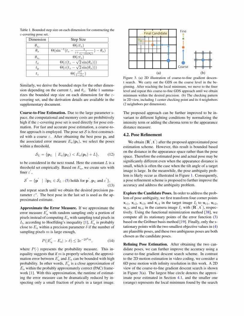
Table 1. Bounded step size on each dimension for constructing theε-covering pose set.

Dimension Step Sizeθzc Θ(εtz)

θx Θ(sin−1(tz − 1ε+ 1

tz−sin(θx)

)− θx)

θzt Θ(εtz)

tx Θ(ε(tz −√

2 sin(θx)))

ty Θ(ε(tz −√

2 sin(θx)))

tz Θ(εt2z

1−εtz )

Similarly, we derive the bounded steps for the other dimen-sion depending on the current tz and θx. Table 1 summa-rizes the bounded step size on each dimension for the ε-covering set, and the derivation details are available in thesupplementary document.

Coarse-to-Fine Estimation. Due to the large parameter s-pace, the computational and memory costs are prohibitivelyhigh if the ε-covering pose set is used directly for pose esti-mation. For fast and accurate pose estimation, a coarse-to-fine approach is employed. The pose set S is first construct-ed with a coarse ε. After obtaining the best pose pb andthe associated error measure Ea(pb), we select the poseswithin a threshold,

SL = {pL | Ea(pL) < Ea(pb) + L}, (12)

to be considered in the next round. Here the constant L is athreshold set empirically. Based on Ea, we create sets withfiner ε

′,

S′

= {p′| ∃pL ∈ SL : (5) holds for p

′,pL and ε

′},(13)

and repeat search until we obtain the desired precision pa-rameter ε∗. The best pose in the last set is used as the ap-proximated estimate.

Approximate the Error Measure. If we approximate theerror measure E

′

a with random sampling only a portion ofpixels instead of computingEa with sampling total pixels inIt, according to Hoeffding’s inequality [1], E

′

a is probablyclose to Ea within a precision parameter δ if the number ofsampling pixels m is large enough,

P (|E′

a − Ea| > δ) ≤ 2e−2δ2m, (14)

where P (·) represents the probability measure. This in-equality suggests that ifm is properly selected, the approxi-mation error between E

′

a and Ea can be bounded with highprobability. In other words, E

′

a is a close approximation ofEa within the probably approximately correct (PAC) frame-work [1]. With this approximation, the runtime of estimat-ing the error measure can be dramatically reduced by in-specting only a small fraction of pixels in a target image.

Coarse

FineFinal Candidate

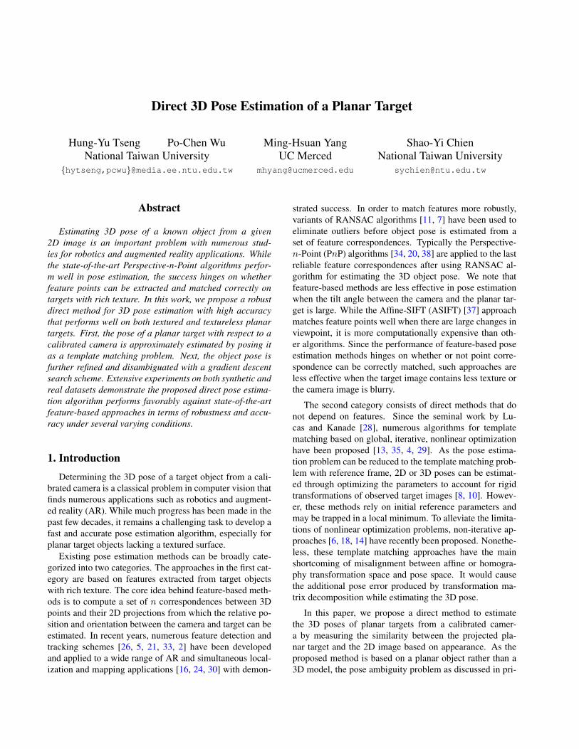
(a) (b)Figure 3. (a) 2D illustration of coarse-to-fine gradient descen-t search. We carry out the GDS on the coarse level in the be-ginning. After reaching the local minimum, we move to the finerlevel and repeat this coarse-to-fine GDS approach until we obtainminimum within the desired precision. (b) The checking patternin 2D view, including 1 center checking point and its 4 neighnbors(2 neighnbors per dimension).

The proposed approach can be further improved to be in-variant to different lighting conditions by normalizing theintensity term or adding the chroma term to the appearancedistance measure.

4.2. Pose Refinement

We obtain (R′, t′) after the proposed approximated pose

estimation scheme. However, this result is bounded basedon the distance in the appearance space rather than the posespace. Therefore the estimated pose and actual pose may besignificantly different even when the appearance distance issmall, which is often the case when the tilt angle of a targetimage is large. In the meanwhile, the pose ambiguity prob-lem is likely occur as illustrated in Figure 1. Consequently,a pose refinement scheme is proposed to further improve theaccuracy and address the ambiguity problem.

Explore the Candidate Poses. In order to address the prob-lem of pose ambiguity, we first transform four corner pointsxc1, xc2, xc3, and xc4 in the target image It to uc1, uc2,uc3, and uc4 in the camera image Ic with (R

′, t′), respec-

tively. Using the functional minimization method [38], wecompute all its stationary points of the error function (3)based on the Grobner basis method [19]. Finally, only the s-tationary points with the two smallest objective values in (4)are plausible poses, and these two ambiguous poses are bothchosen as the candidate poses.

Refining Pose Estimation. After obtaining the two can-didate poses, we can further improve the accuracy using acoarse-to-fine gradient descent search scheme. In contrastto the 2D motion estimation in video coding, we consider a6D pose motion with infinity resolution in this work. A 2Dview of the coarse-to-fine gradient descent search is shownin Figure 3(a). The largest blue circle denotes the approx-imate pose estimated in Section 4.1, and the smaller one(orange) represents the local minimum found by the search

pattern at the starting ε-precision. As the minimum underthe current precision level is found, we diminish the preci-sion parameter ε and perform gradient descent search againon the next level. This process is repeated until we obtainthe local minimum under the desired precision parameterε∗. Finally, the pose with smaller Ea is chosen from thetwo refined candidate poses.

The 2D view of the checking pattern in the coarse-to-fine GDS scheme [25] are shown in Figure 3(b). It isformed by 13 checking points, including the center pointand its 12 neighbors. These 12 neighbors are ε-awayfrom the center separately in the 6D pose space. Letpc = [θzc , θx, θzt , tx, ty, tz]

> be the center point of thechecking pattern in the pose space and Pc be the 6 ×13 matrix with repeating pc in a row. Also let sε =[sθzc , sθx , sθzt , stx , sty , stz ]

> be the step size listed in Ta-ble 1 with precision parameter ε and Sε be the 6×13 matrixwith repeating sε in a row. The mathematical description ofthe checking pattern M can then be written as

M = Pc + D ◦ Sε, (15)

where

D =

0 1 −1 0 0 . . . 0 00 0 0 1 −1 . . . 0 00 0 0 0 0 . . . 0 00 0 0 0 0 . . . 0 00 0 0 0 0 . . . 0 00 0 0 0 0 . . . 1 −1

(16)

and ◦ represents the Hadamard product. Each column in Mrepresents one of the checking points within the checkingpattern. The main steps of the proposed pose estimationmethod are summarized in Algorithm 1.

5. Experimental ResultsWe experimentally evaluate the proposed algorithm for

the 3D pose estimation problem using both synthetic andbenchmark datasets, and compare it with the feature-basedschemes. Through some preliminary experiments, we findthe SIFT [26] method performs better than other alternativefeatures in terms of repeatability and accuracy. Similar ob-servations can also be found in [12]. As the ASIFT [37]method is considered the state-of-the-art affine-invariantmethod to find correspondences under large view change,we use both the SIFT and ASIFT methods in the comparedfeature-based schemes. The RANSAC-based method [11]is then used to eliminate outliers before object pose is es-timated by the PnP algorithms. It has been shown that, a-mong the PnP algorithms [34, 20, 38, 17], the OPnP [38]algorithm achieves the state-of-the-art results in terms of ef-ficiency and precision. Therefore we use the OPnP algorith-m as the pose estimator in the feature-based schemes.

Algorithm 1 Proposed Direct 3D Pose EstimationInput: Target image It, camera image Ic, intrinsic param-

eters, and precision parameters ε∗c , ε∗f .

Output: Estimated pose result p∗.1: Create an ε-covering pose set S.2: Find pb from S with E

′

a according to (14).3: while ε > ε∗c do4: Obtain the set SL according to (12);5: Diminish ε;6: Replace S according to (13);7: Find pb from S with E

′

a according to (14);8: end while9: Explore the candidate poses p1 and p2 with pb.

10: for i = 1→ 2 do11: Let pc = pi and εi = ε12: while εi > ε∗f do13: Find pb from (15) with E

′

a according to (14).14: if pc 6= pb then15: pc = pb16: else17: Diminish εi;18: end if19: end while20: Let pi = pc21: end for22: Return the pose p∗ with smaller Ea from p1 and p2

We run all codes in MATLAB on a desktop computerwith 3.4 GHz CPU and 16 GB RAM. Table 2 shows av-erage runtimes for different algorithms. The source codeand datasets will be made available to the public. Due tothe space limit, we leave more results in the supplementalmaterial.

Given the true rotation matrix R and translation vectort, we compute the rotation error of the estimated rotationmatrix R by ER(degree) = acosd((Tr(R> · R)− 1)/2),where acosd(·) represents the arc-cosine operation in de-grees. The translation error of the estimated translation vec-tor t is measured by the relative difference between t and tdefined as Et(%) = ‖t − t‖/‖t‖ × 100. We define a poseto be successfully estimated if its both errors are under pre-defined thresholds. We use δR = 20◦ and δt = 10% as thethreshold on rotation error and translation error empirically,as shown in Figure 4. The success rate (SR) is defined as thepercentage of the successfully estimated poses within eachtest condition.

5.1. Synthetic Images

We use a set of synthetic images consisting of 8400 testimages for experiments, including 21 different test condi-tions. Each test image is generated from a warping tem-plate image according to the randomly generated pose with

Table 2. Average runtimes for three approaches on synthetic and real test data. Numbers in parentheses represents the average steps ofchecking pattern in the refinement approach. Although SIFT-based Approach is the fastest method among these three different schemes,its performance is quite limited.

Data TypeSIFT-based Approach ASIFT-based Approach Proposed Direct Method

SIFT RANSAC OPnP Total ASIFT RANSAC OPnP Total Approximated Refinement Total

Synthetic 10.56 s. 0.08 s. 0.02 s. 10.67 s. 46.45 s. 0.07 s. 0.02 s. 46.58 s. 38.35 s. (26.3) 2.16 s. 40.51 s.

Real 5.09 s. 0.08 s. 0.02 s. 5.19 s. 24.91 s. 0.09 s. 0.02 s. 25.08 s. 35.13 s. (19.5) 1.29 s. 36.42 s.

0 5000 10000 150000

20

50

100

150

200

250

300

Image Index

Rot

atio

n E

rror

(D

egre

e)

SIFT ASIFT Direct

0 5000 10000 150000

10

50

100

150

Image Index

Tra

nsla

tion

Err

or (

%)

SIFT ASIFT Direct

Figure 4. Distributions of rotation and translation errors over ex-periments. The horizontal lines correspond to the thresholds usedto detect unsuccessfully estimated poses. There is a total of15, 289 poses estimated by each pose estimation approach.

Background ImagesTemplates Test Images

Figure 5. The test image was generated from a warping templateimage according to the randomly generated pose on randomly cho-sen background image.

tilt angle in the range [0◦, 75◦] in a randomly chosen back-ground image, as shown in Figure 5. The template imagesize is 640 × 480. These templates are classified into fourdifferent classes, namely “Low Texture”, “Repetitive Tex-ture”, “Normal Texture”, and “High Texture” [23] as shownfrom top to bottom in Figure 5. Each class is represented bytwo targets. The background images are acquired from thedatabase [15] and resized to 800× 600 pixels.

Normal Conditions. The pose estimation results of theSIFT-based, ASIFT-based, and the proposed direct meth-ods using the undistorted test images are shown in Table 3.Each test condition contains the average rotation error ER,translation error Et, and success rate. The evaluation re-sults show that although the proposed method is sometimesslightly less accurate than the feature-based approaches, itperforms more robustly with different templates. Althoughthe SIFT-based approach can detect and match the featuresaccurately under small tilt angle, it frequently fails in the ex-periments when the template undergoes large pose change.In most cases, the feature-based approaches cannot correct-ly estimate the pose of textureless template images.

0.2 0.4 0.8 1.6 3.3 6.8 14 28 58 1200

5

10

15

20

25

30

Rotation Error (Degree)

Per

cent

age

of P

oses

(%

)

Without RefinementWith Refinement

0.1 0.2 0.5 1.1 2.3 4.7 10 21 44 930

5

10

15

20

25

30

35

Translation Error (%)

Per

cent

age

of P

oses

(%

)

Without RefinementWith Refinement

Figure 6. Pose estimation results with and without refinement ap-proaches. The average value of rotation and translation error areboth reduced by the refinement approach.

Varying Conditions. We further evaluate the proposedmethods using all templates with five degradation levels:Gaussian blur with kernel width of {1, 2, 3, 4, 5} pixels,JPEG compression with the quality parameter set to {90,80, 70, 60, 50}, intensity change with pixel intensity s-calar parameter set to {0.9,0.8,0.7,0.6,0.5}, and tilt anglein the range of {[0◦15◦), [15◦30◦), [30◦45◦), [45◦60◦), and[60◦75◦)}. The results are shown in Figure 7. The proposedalgorithm outperforms the other two feature-based methodswith blurry images. All three approaches are able to dealwith certain levels of distortion in intensity or JPEG com-pression noise. The SIFT-based approach performs wellwhen the tilt angle is small since the marker images arenot perspective distorted in the camera images. In the otherconditions, however, the proposed algorithm and the ASFITmethod are able to estimate 3D poses relatively well. In thissynthetic image experiment, the proposed direct methodachieves an overall success rate of 95.62%, while SIFT-based and ASIFT-based approaches achieve success ratesof 47.62% and 74.74% respectively.

Refinement Analysis. To improve the accuracy of our poseestimation algorithm, we propose a refinement approach asdescribed in Section 4.2. Pose estimation results (i.e., ro-tation and translation error) with and without the refine-ment approach are shown in Figure 6. The rotation andtranslation error can be reduced averagely by −0.258◦ and−0.233% respectively with proposed refinement scheme.

To demonstrate the proposed algorithm is able to disam-biguate among plausible poses, we design another experi-ment conducted as follows: For each test, we choose a testimage from the synthetic images. The template image inthis test image is warped according to pose pt. An am-biguous pose pa is then determined from pt using the func-tional minimization method [38]. One of the two plausi-

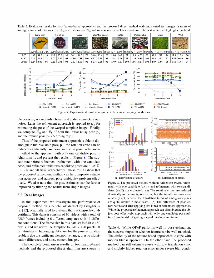
Table 3. Evaluation results for two feature-based approaches and the proposed direct method with undistorted test images in terms ofaverage number of rotation error ER, translation error Et, and success rate in each test condition. The best values are highlighted in bold.

Bump Sign

Stop Sign

Lucent

MacMini Board

Isetta

Philadelphia

Grass

Wall

𝐸𝐑(°) 𝐸𝐭(%) SR(%) 𝐸𝐑(°) 𝐸𝐭(%) SR(%) 𝐸𝐑(°) 𝐸𝐭(%) SR(%) 𝐸𝐑(°) 𝐸𝐭(%) SR(%) 𝐸𝐑(°) 𝐸𝐭(%) SR(%) 𝐸𝐑(°) 𝐸𝐭(%) SR(%) 𝐸𝐑(°) 𝐸𝐭(%) SR(%) 𝐸𝐑(°) 𝐸𝐭(%) SR(%)

SIFT 100 54.8 10 69.2 35.3 38 30.1 16.5 72 28.0 13.4 78 20.6 16.2 82 13.5 4.57 90 97.3 212 24 17.1 27.3 86

ASIFT 72.1 24.3 22 5.07 0.74 96 1.90 0.38 100 6.37 2.59 96 2.08 0.49 98 1.16 0.35 100 51.2 16.7 52 2.76 0.36 96

Direct 3.84 0.80 96 2.81 0.91 98 2.62 1.06 98 5.37 2.56 96 1.49 0.87 100 1.95 0.87 100 2.87 1.06 96 6.68 1.64 94

0

20

40

60

80

100

120

140

1 2 3 4 5Ro

tati

on

Err

or

(Deg

ree)

Distortion Level

Blur (SIFT) Blur (ASIFT) Blur (Direct) JPEG (SIFT) JPEG (ASIFT) JPEG (Direct)

Intensity (SIFT) Intensity (ASIFT) Intensity (Direct) Tilt (SIFT) Tilt (ASIFT) Tilt (Direct)

0

20

40

60

80

100

1 2 3 4 5

Tran

slat

ion

Err

or

(%)

Distortion Level

0

20

40

60

80

100

120

1 2 3 4 5

Succ

essf

ul R

ate

(%)

Distortion Level

Figure 7. Experimental results on synthetic data under varying conditions.

ble poses p′

a is randomly chosen and added some Gaussiannoise. Later the refinement approach is applied to p

′

a forestimating the pose of the warped template image. Finally,we compute ER and Et of both the initial noisy pose p

′

a

and the refined pose pr according to pt.Thus, if the proposed refinement approach is able to dis-

ambiguate the plausible pose p′

a, the rotation error can bereduced significantly. We compare the proposed refinemen-t method to the approach with only one candidate pose inAlgorithm 1, and present the results in Figure 8. The suc-cess rate before refinement, refinement with one candidatepose, and refinement with two candidate poses are 51.26%,51.19% and 90.34%, respectively. These results show thatthe proposed refinement method can help improve estima-tion accuracy and address pose ambiguity problem effec-tively. We also note that the pose estimates can be furtherimproved by filtering the results from single images.

5.2. Real Images

In this experiment we investigate the performance ofproposed method on a benchmark dataset by Gauglitz etal. [12], originally used to evaluate the tracking-related al-gorithms. This dataset consists of 96 videos with a total of6889 frames including 6 different templates with 16 differ-ent conditions. The frame size in this data set is 640× 480pixels, and we resize the template to 570 × 420 pixels. Itis definitely a challenging database for the pose estimationproblem due to significant viewpoint change, drastic illumi-nation difference, and noisy camera images.

The complete comparison results of two feature-basedmethods and the proposed direct algorithm are shown in

0.1 0.2 0.4 0.8 1.9 4.3 9.9 23 52 1190

0.1

0.2

0.3

0.4

0.5

Rotation Error in Degree (log scale)

Per

cent

age

of P

oses

(%

)

w/ow/ 1w/ 2

0 1000 2000 3000 4000 5000−200

−100

0

100

200

Image Index

Diff

eren

ce o

f Rot

atio

n E

rror

(D

egre

e)

Refinement with 1 Candidate PoseRefinement with 2 Candidate Poses

0.1 0.2 0.4 0.9 2 4.4 9.5 21 45 980

0.1

0.2

0.3

0.4

0.5

Translation Error in % (log scale)

Per

cent

age

of P

oses

(%

)

w/ow/ 1w/ 2

0 1000 2000 3000 4000 5000−40

−20

0

20

40

60

80

100

Image Index

Diff

eren

ce o

f Tra

nsla

tion

Err

or (

%)

Refinement with 1 Candidate PoseRefinement with 2 Candidate Poses

(a) Distribution of errors. (b) Difference of errors.

Figure 8. The proposed method without refinement (w/o), refine-ment with one candidate (w/ 1), and refinement with two candi-dates (w/ 2) are evaluated. (a) The rotation errors are reduceddrastically in the ambiguous cases, but the translation errors arerelatively not, because the translation terms of ambiguous posesare quite similar in most cases. (b) The difference of pose er-rors before and after applying two kinds of refinement approaches.While the proposed refinement approach can disambiguate the ob-ject pose effectively, approach with only one candidate pose suf-fers from the risk of getting trapped into local minimum.

Table 4. While OPnP performs well in pose estimation,the success hinges on whether feature can be well matched.The difficulty of the feature-based approaches to cope withmotion blur is apparent. On the other hand, the proposedmethod can still estimate poses with low translation errorand slightly higher rotation error under severe blur condi-

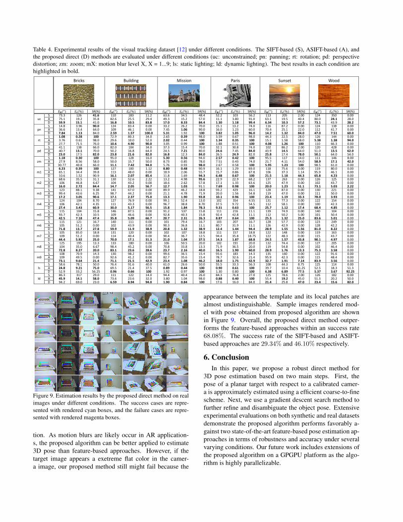
Table 4. Experimental results of the visual tracking dataset [12] under different conditions. The SIFT-based (S), ASIFT-based (A), andthe proposed direct (D) methods are evaluated under different conditions (uc: unconstrained; pn: panning; rt: rotation; pd: perspectivedistortion; zm: zoom; mX: motion blur level X, X = 1...9; ls: static lighting; ld: dynamic lighting). The best results in each condition arehighlighted in bold.

Bricks

Building

Mission

Paris

Sunset

Wood

𝐸𝐑(°) 𝐸𝐭(%) SR(%) 𝐸𝐑(°) 𝐸𝐭(%) SR(%) 𝐸𝐑(°) 𝐸𝐭(%) SR(%) 𝐸𝐑(°) 𝐸𝐭(%) SR(%) 𝐸𝐑(°) 𝐸𝐭(%) SR(%) 𝐸𝐑(°) 𝐸𝐭(%) SR(%)

uc S 73.3 126 41.6 110 183 11.2 63.6 34.5 48.4 52.2 103 56.2 113 205 2.00 124 350 0.00 A 75.1 19.2 35.8 82.6 25.5 29.4 49.3 15.2 57.0 11.1 3.80 91.0 63.1 19.5 40.4 80.0 24.1 28.0 D 59.9 15.1 41.0 16.8 10.5 83.8 17.0 8.33 84.4 1.30 1.18 99.4 6.34 10.3 57.2 73.1 43.9 28.2

pn S 14.8 3.96 90.0 124 83.4 0.00 33.2 26.2 70.0 15.1 13.2 74.0 116 87.2 0.00 124 138 0.00 A 36.6 13.4 64.0 109 46.1 0.00 7.45 1.06 90.0 16.0 1.23 60.0 70.4 25.1 22.0 112 41.7 0.00 D 7.84 1.13 84.0 2.59 1.57 100.0 5.31 1.92 100 3.82 1.05 96.0 14.2 1.32 84.0 47.0 7.51 60.0

rt S 1.08 0.28 100 72.9 80.3 34.0 2.65 0.39 98.0 3.59 0.67 98.0 44.3 22.5 28.0 126 144 0.00 A 3.76 0.61 98.0 29.6 10.0 52.0 2.02 0.44 100 1.34 0.35 100 15.1 1.58 58.0 5.38 1.38 94.0 D 27.7 71.5 76.0 10.6 4.90 90.0 3.05 0.99 100 1.88 0.51 100 4.08 1.26 100 110 66.3 0.00

pd S 41.1 138 66.0 82.0 104 34.0 37.3 15.4 70.0 32.1 30.8 74.0 102 86.2 2.00 120 428 0.00 A 40.7 13.1 70.0 50.2 16.8 64.0 24.5 7.21 80.0 24.6 7.45 84.0 43.9 14.5 64.0 51.0 13.5 62.0 D 23.0 17.5 82.0 23.8 21.6 82.0 16.8 12.3 84.0 26.5 24.9 82.0 25.8 17.4 78.0 50.1 64.0 54.0

zm S 1.18 0.30 100 95.0 128 16.0 5.30 0.56 94.0 2.57 0.42 100 95.5 117 14.0 111 146 8.00 A 27.9 8.56 58.0 50.0 15.7 50.0 8.73 0.85 78.0 7.51 0.43 74.0 21.7 4.11 54.0 58.9 17.1 42.0 D 30.77 40.8 66.0 11.1 7.42 94.0 5.76 0.93 98.0 2.67 0.58 100 5.95 1.23 100 98.5 61.0 0.00

m1 S 6.23 0.39 100 127 100 1.12 8.80 0.48 90.9 16.1 1.29 69.0 118 75.6 0.00 119 80.0 0.00 A 65.1 34.4 39.8 113 48.0 0.00 18.9 2.06 55.7 15.7 0.86 67.8 106 37.3 1.14 95.9 46.1 0.00 D 10.6 1.52 90.9 16.1 2.07 85.4 11.8 1.69 94.3 6.48 0.67 100 21.5 1.18 44.3 65.8 4.23 0.00

m2 S 68.6 35.5 31.1 130 52.6 2.22 13.2 4.98 95.6 22.9 22.9 68.2 137 263 0.00 126 125 0.00 A 106 46.8 6.67 104 43.2 0.00 18.6 2.62 57.8 17.1 1.33 63.6 125 47.9 0.00 102 43.7 0.00 D 16.0 2.72 84.4 14.7 2.05 56.7 12.7 1.03 91.1 7.69 0.98 100 20.0 1.23 51.1 73.1 5.03 2.22

m3 S 123 88.1 9.38 141 67.0 0.00 89.9 46.2 18.8 93.2 429 16.1 128 87.0 0.00 130 221 0.00 A 99.4 43.6 6.25 98.7 44.2 0.00 21.1 4.78 71.9 20.0 1.56 54.8 119 47.0 0.00 111 50.0 0.00 D 17.2 3.05 90.6 17.1 2.37 75.0 13.3 1.90 93.8 10.1 0.96 100 23.4 1.19 33.3 78.0 3.93 0.00

m4 S 124 104 8.70 127 76.9 0.00 99.1 52.4 13.0 102 354 4.55 131 77.3 0.00 122 154 0.00 A 106 42.1 4.35 111 43.3 0.00 96.7 38.8 8.70 37.5 9.72 54.5 112 58.1 0.00 100 42.3 0.00 D 27.4 3.43 60.9 30.0 5.17 56.5 15.8 1.84 78.3 9.31 0.63 100 25.7 1.12 17.4 68.4 4.85 0.00

m5 S 115 104 15.8 146 87.5 0.00 91.2 537 15.8 111 216 11.1 139 74.9 0.00 140 104 0.00 A 93.7 42.3 10.5 109 46.6 0.00 92.8 40.3 15.8 92.4 42.8 11.1 112 50.2 5.00 101 50.4 0.00 D 42.5 7.18 47.4 35.8 5.09 66.7 20.7 2.31 26.3 8.87 0.64 100 25.3 1.32 25.0 83.6 5.01 0.00

m6 S 115 121 16.7 140 111 0.00 101 79.4 16.7 103 207 16.7 128 57.7 0.00 123 249 0.00 A 105 51.2 0.00 102 43.9 0.00 90.3 36.8 11.1 80.7 31.9 11.1 126 42.9 0.00 128 42.2 0.00 D 71.8 13.7 27.8 59.9 11.9 38.9 20.8 1.32 38.9 12.4 1.44 94.4 28.9 1.55 5.56 81.0 8.22 0.00

m7 S 105 85.0 18.8 131 120 0.00 102 107 18.8 111 157 18.8 122 148 0.00 119 163 0.00 A 109 51.2 0.00 114 40.4 0.00 90.4 36.7 12.5 94.4 35.8 18.75 122 48.3 0.00 115 43.7 0.00 D 44.4 5.92 25.0 70.0 17.1 31.3 21.0 1.04 37.5 14.3 1.87 68.8 24.5 1.57 43.8 90.1 4.97 0.00

m8 S 125 195 13.3 133 180 0.00 106 50.5 20.0 102 191 20.0 132 74.4 0.00 127 205 0.00 A 104 35.0 6.67 98.4 45.2 0.00 70.8 33.8 13.3 71.9 36.5 20.0 119 54.8 0.00 102 46.4 0.00 D 72.8 8.27 20.0 83.1 23.6 28.6 23.7 2.16 40.0 16.5 1.90 60.0 28.9 1.76 13.3 75.3 3.58 0.00

m9 S 108 70.9 14.3 130 98.2 0.00 99.6 36.5 15.4 93.6 183 14.3 135 160 0.00 122 91.6 0.00 A 109 49.5 0.00 92.6 41.2 0.00 82.7 35.6 15.4 78.7 32.6 21.4 95.9 42.3 0.00 115 48.4 0.00 D 73.1 9.64 21.4 71.1 21.5 42.9 23.4 1.08 46.2 18.0 1.75 42.9 32.7 1.91 7.14 83.9 3.56 0.00

ls S 58.6 78.1 50.0 76.4 91.6 40.0 61.0 26.6 50.0 55.5 33.3 56.3 108 44.3 8.75 125 114 0.00 A 24.8 9.21 75.0 69.5 21.4 37.5 0.89 0.44 100 0.90 0.61 100 39.7 10.4 61.25 52.5 18.3 51.3 D 52.9 33.2 56.25 0.96 0.66 100 1.92 0.97 100 1.30 0.80 100 6.38 6.89 77.5 5.37 3.67 92.25

ld S 86.3 317 29.0 111 122 14.0 94.4 40.4 26.0 84.3 76.8 27.0 125 78.6 2.00 126 182 0.00 A 45.9 14.1 58.0 73.6 23.6 32.0 3.80 1.04 98.0 0.88 0.40 100 55.4 19.2 45.0 51.3 20.2 50.0 D 94.2 69.0 23.0 6.59 8.94 94.0 1.90 0.84 100 17.6 16.0 84.0 21.4 25.8 47.0 23.4 15.6 82.0

Figure 9. Estimation results by the proposed direct method on realimages under different conditions. The success cases are repre-sented with rendered cyan boxes, and the failure cases are repre-sented with rendered magenta boxes.

tion. As motion blurs are likely occur in AR application-s, the proposed algorithm can be better applied to estimate3D pose than feature-based approaches. However, if thetarget image appears a exetreme flat color in the camer-a image, our proposed method still might fail because the

appearance between the template and its local patches arealmost undistinguishable. Sample images rendered mod-el with pose obtained from proposed algorithm are shownin Figure 9. Overall, the proposed direct method outper-forms the feature-based approaches within an success rate68.08%. The success rate of the SIFT-based and ASIFT-based approaches are 29.34% and 46.10% respectively.

6. ConclusionIn this paper, we propose a robust direct method for

3D pose estimation based on two main steps. First, thepose of a planar target with respect to a calibrated camer-a is approximately estimated using a efficient coarse-to-finescheme. Next, we use a gradient descent search method tofurther refine and disambiguate the object pose. Extensiveexperimental evaluations on both synthetic and real datasetsdemonstrate the proposed algorithm performs favorably a-gainst two state-of-the-art feature-based pose estimation ap-proaches in terms of robustness and accuracy under severalvarying conditions. Our future work includes extensions ofthe proposed algorithm on a GPGPU platform as the algo-rithm is highly parallelizable.

References[1] Y. S. Abu-Mostafa, M. Magdon-Ismail, and H.-T. Lin.

Learning from data. AMLBook, 2012. 4[2] A. Alahi, R. Ortiz, and P. Vandergheynst. Freak: Fast retina

keypoint. In CVPR, 2012. 1[3] B. Alexe, V. Petrescu, and V. Ferrari. Exploiting spatial over-

lap to efficiently compute appearance distances between im-age windows. In NIPS, pages 2735–2743, 2011. 2

[4] S. Baker and I. Matthews. Equivalence and efficiency of im-age alignment algorithms. In CVPR, 2001. 1

[5] H. Bay, A. Ess, T. Tuytelaars, and L. Van Gool. Speeded-uprobust features (surf). Computer Vision and Image Under-standing, 110(3), 2008. 1

[6] Y.-T. Chi, J. Ho, and M.-H. Yang. A direct method for esti-mating planar projective transform. In ACCV. 2011. 1

[7] O. Chum and J. Matas. Matching with prosac-progressivesample consensus. In CVPR, 2005. 1

[8] A. Crivellaro and V. Lepetit. Robust 3d tracking with de-scriptor fields. In CVPR, 2014. 1

[9] D. Eberly. Euler angle formulas. Geometric Tools, LLC,Technical Report, 2008. 3

[10] J. Engel, T. Schops, and D. Cremers. Lsd-slam: Large-scaledirect monocular slam. In ECCV. 2014. 1

[11] M. A. Fischler and R. C. Bolles. Random sample consen-sus: a paradigm for model fitting with applications to imageanalysis and automated cartography. Communications of theACM, 24(6):381–395, 1981. 1, 5

[12] S. Gauglitz, T. Hollerer, and M. Turk. Evaluation of interestpoint detectors and feature descriptors for visual tracking.IJCV, 94(3):335–360, 2011. 5, 7, 8

[13] G. D. Hager and P. N. Belhumeur. Efficient region trackingwith parametric models of geometry and illumination. IEEETPAMI, 20(10):1025–1039, 1998. 1

[14] J. F. Henriques, P. Martins, R. F. Caseiro, and J. Batista. Fasttraining of pose detectors in the fourier domain. In NIPS,2014. 1

[15] H. Jegou, M. Douze, and C. Schmid. Hamming embeddingand weak geometric consistency for large scale image search.In ECCV. 2008. 2, 6

[16] G. Klein and D. Murray. Parallel tracking and mapping forsmall ar workspaces. In ISMAR, 2007. 1

[17] L. Kneip, H. Li, and Y. Seo. Upnp: An optimal o (n) solutionto the absolute pose problem with universal applicability. InECCV. 2014. 5

[18] S. Korman, D. Reichman, G. Tsur, and S. Avidan. Fast-match: Fast affine template matching. In CVPR, 2013. 1,2, 3

[19] Z. Kukelova, M. Bujnak, and T. Pajdla. Automatic generatorof minimal problem solvers. In ECCV. 2008. 2, 4

[20] V. Lepetit, F. Moreno-Noguer, and P. Fua. Epnp: An accurateO(n) solution to the pnp problem. IJCV, 81(2), 2009. 1, 5

[21] S. Leutenegger, M. Chli, and R. Y. Siegwart. BRISK: BinaryRobust Invariant Scalable Keypoints. In ICCV, 2011. 1

[22] S. Li and C. Xu. Efficient lookup table based camera poseestimation for augmented reality. Computer Animation andVirtual Worlds, 22(1):47–58, 2011. 2

[23] S. Lieberknecht, S. Benhimane, P. Meier, and N. Navab.A dataset and evaluation methodology for template-basedtracking algorithms. In ISMAR, 2009. 6

[24] H. Lim, S. N. Sinha, M. F. Cohen, and M. Uyttendaele. Real-time image-based 6-dof localization in large-scale environ-ments. In CVPR, 2012. 1

[25] L.-K. Liu and E. Feig. A block-based gradient descent searchalgorithm for block motion estimation in video coding. IEEETCSVT, 6(4):419–422, 1996. 2, 5

[26] D. G. Lowe. Distinctive image features from scale-invariantkeypoints. IJCV, 60(2), 2004. 1, 5

[27] C. Lu, G. Hager, and E. Mjolsness. Fast and globally con-vergent pose estimation from video images. IEEE TPAMI,22(6):610–622, 2000. 2

[28] B. D. Lucas, T. Kanade, et al. An iterative image registra-tion technique with an application to stereo vision. In IJCAI,volume 81, pages 674–679, 1981. 1

[29] E. Malis. Improving vision-based control using efficien-t second-order minimization techniques. In ICRA, 2004. 1

[30] R. Mur-Artal and J. D. Tardos. Fast relocalisation and loopclosing in keyframe-based slam. In ICRA, 2014. 1

[31] D. Oberkampf, D. F. DeMenthon, and L. S. Davis. Iterativepose estimation using coplanar points. In CVPR, 1993. 2

[32] O. Pele and M. Werman. Accelerating pattern matching orhow much can you slide? In ACCV. 2007. 2

[33] E. Rublee, V. Rabaud, K. Konolige, and G. Bradski. Orb: anefficient alternative to sift or surf. In ICCV, 2011. 1

[34] G. Schweighofer and A. Pinz. Robust Pose Estimation froma Planar Target. IEEE TPAMI, 28(12), 2006. 1, 2, 5

[35] H.-Y. Shum and R. Szeliski. Construction of panoramic im-age mosaics with global and local alignment. In PanoramicVision, pages 227–268. 2001. 1

[36] P.-C. Wu, Y.-H. Tsai, and S.-Y. Chien. Stable pose trackingfrom a planar target with an analytical motion model in real-time applications. In MMSP, 2014. 2

[37] G. Yu and J.-M. Morel. Asift: A new framework for ful-ly affine invariant image comparison. Image Processing OnLine, 2011. 1, 5

[38] Y. Zheng, Y. Kuang, S. Sugimoto, K. Astrom, and M. Oku-tomi. Revisiting the PnP Problem: A Fast, General and Op-timal Solution. In ICCV, 2013. 1, 2, 4, 5, 6

[39] C. Zhu, X. Lin, and L.-P. Chau. Hexagon-based searchpattern for fast block motion estimation. IEEE TCSVT,12(5):349–355, 2002. 2

[40] S. Zhu and K.-K. Ma. A new diamond search algorithm forfast block-matching motion estimation. IEEE TIP, 9(2):287–290, 2000. 2