arX

iv:h

ep-t

h/04

1021

6v2

5 N

ov 2

004

Yukawa Institute Kyoto YITP-04-56

OIQP-04-3

Oct. 2004

Dirac Sea for Bosons I

— Formulation of Negative Energy Sea for Bosons — ∗

Holger B. Nielsen

Niels Bohr Institute,

University of Copenhagen, 17 Blegdamsvej,

Copenhagen ø, DK 2100, Denmark

and

Masao Ninomiya†

Yukawa Institute for Theoretical Physics

Kyoto University, Sakyo-ku, Kyoto 606-8502, Japan

Abstract

It is proposed to make formulation of second quantizing a bosonic theory bygeneralizing the method of filling the Dirac’s negative energy sea for fermions. Weinterpret that the correct vacuum for the bosonic theory is obtained by addingminus one boson to each single particle negative energy states while the positiveenergy states are empty. The boson states are divided into two sectors ; the usualpositive sector with positive and zero numbers of bosons and the negative sectorwith negative number of bosons. Once it comes into the negative sector it cannotreturn to the usual positive sector by ordinary interaction due to a barrier.

It is suggested to use as a playground model in which the filling of emptyfermion Dirac sea and the removal of boson from the negative energy states arenot yet performed. We put forward such a naive vacuum world in the presentpaper. The successive paper[1] will concern various properties: Analyticity of thewave functions, interaction and a CPT-like Theorem in the naive vacuum world.

∗This paper is the first part of the revised version of ref. [2].†Also, Okayama Institute for Quantum Physics, Kyo-yama 1-9-1, Okayama City 700-0015,

Japan

1. Introduction

There has been a wellknown method, though not popular nowadays, to secondquantize relativistic fermion by imagining that there is a priori so called naivevacuum in which there is no, neither positive energy nor negative energy, fermionpresent. However this vacuum is unstable and the negative energy state gets filledwhereby the Dirac sea is formed [3]1. This method of filling at first empty Diracsea seems to make sense only for fermions for which there is Pauli principle. In thisway “correct vacuum” is formed out of “naive vacuum”, the former well functioningphenomenologically. Formally by filling Dirac sea we define creation operators

b+(⇀p, s, ω) for holes which is equivalent to destruction operators a(− ⇀

p,−s,−ω)for negative energies −ω and altogether opposite quantum numbers. This formalrewriting can be used also for bosons, but we have never heard the associated fillingof the negative energy states.

As a matter of fact the truely new content and the main motivation of thepresent paper is to present an idea as to how the 2nd quantized field theory inthe boson case looks analogous to the fermion system before the Dirac sea is filledout. Although this bosonic theory analogous to the empty Dirac sea for fermionshas the serious drawbacks: It has an indefinite “Hilbert space” as its Fock space.Furthermore it possesses no bottom in the spectrum of the Hamiltonian. However ithas much nicer features than the true vacuum theory in which the negative energystates are completely filled: Existence of position eigenstates and description interms of finite dimensional wave functions.

At the very end when the true vacuum for the case of bosons is realized accord-ing to our method presented in this paper, we will come exactly the same theoryas the usual one. Thus our approach cannot be incorrect, but the true vacuumtheory itself may not provide new results.

However “the naively quantized theory”, which is an analogue of the unfilledDirac sea for fermions, is nice to think about because it turns out to be a world inwhich only a few particles can be described by wave functions of the positions ofthese few particles. Remarkably, contrary to usual relativistic theories, the particlesin the “naive vaccum world” have position eigenstates. They can be achieved onlyas superposition of positive and negative energy eigenstates.

The problem of passage from the naive vacuum world to the usual theory in-volves, as already mentioned, addition of “minus one boson” to each negativeenergy state. In the following section 2, we shall concretize how such idea of anegative number of bosons can be thought upon mathematically by treating theharmonic oscillator which is brought in correspondence with a single particle stateunder the usual second quantization. We make an extension of the spectrumwith the excitation number n = 0, 1, 2, . . . to the one with negative integer valuesn = −1,−2. . . .. This extension can be performed by requiring that the wave func-tion ψ(x) should be analytic in the whole complex x plane except for an essentialsingularity at x = ∞. This requirement is a replacement to the usual condition on

1See for example [4] for historical account.

– 2 –

the norm of the finite Hilbert space∫∞−∞ |ψ(x)|2dx <∞. The outcome of the study

is that the harmonic oscillator has the following two sectors : 1) the usual positivesector with positive and zero number of particles, and 2) the negative sector withthe negative number of particles. The latter sector has indefinite Hilbert product.

But we would like to stress that there is a barrier between the usual positivesector and the negative sector. Due to the barrier it is impossible to pass fromone sector to the other with usual polynomial interactions. This is due to someextrapolation of the wellknown laser effect, which make easy to fill an alreadyhighly filled single particle state for bosons. This laser effect may become zerowhen an interaction tries to have the number of particles pass the barrier. In thisway we may explain that the barrier prevents us from observing a negative numberof bosons.

It may be possible to use as a playground a formal world in which one hasneither yet filled the usual Dirac sea of fermions nor performed the one bosonremoval from the negative energy state. We shall indeed study such a playgroundmodel referred to as the naive vacuum model. Particularly we shall provide ananalogous theorem to the CPT theorem 2, since the naive vacuum is not CPTinvariant for both fermions and bosons. At first one might think that a strongreflection without associated inversion of operator order might be good enough.But it turns out this has the unwanted feature that the sign of the interactionenergy is not changed. This changing the sign is required since under strongreflection the sign of all energies should be switched. To overcome this problemwe propose the CPT-like symmetry for the naive vacuum world to include furthera certain analytic continuation. This is constructed by applying a certain analyticcontinuation around branch points which appear in the wave function for each pairof particles. It is presupposed that we can restrict our attention to such a family ofwave function as the one with sufficiently good physical properties. The argumentand proof of CPT-like theorem is deferred to the successive paper[1].

We put forward a physical picture that may be of value in developing an intu-ition on naive vacuum world. In fact investigation of naive vacuum world may bevery attractive because the physics there is quantum mechanics of finite numberof particles. Furthermore the theory is piecewise free in the sense that relativisticinteractions become of infinitely short range. Thus the support that there are in-teractions is null set and one may say that the theory is free almost everywhere.But the very local interactions make themselves felt only via boundary conditionswhere two or more particles meet. This makes the naive vacuum world a theo-retical playground. However it suffers from the following severe drawbacks from aphysical point of view :

• No bottom in the Hamiltonian

• Negative norm square states

• Pairs of particles with tachyonically moving center of mass

2The CPT theorem is well explained in [5]

– 3 –

• It is natural to work with “anti-bound states” rather that bound states inthe negative energy regime.

What we really want to present in the present article is a more dramatic for-mulation of relativistic second quantization of boson theory and one may think ofit as a quantization procedure. We shall formulate below the shift of vacuum forbosons as a shift of boundary conditions in the wave functional formulation of thesecond quantized theory.

But, using the understanding of second quantization of particles along the waywe describe, could we get a better understanding as to how to second quantizestrings? This is our original motivation of the present work. In the oldest attemptto make string field theory by Kaku and Kikkawa [6] the infinite momentum framewas used. To us it looks like an attempt to escape the problem of the negativeenergy states. But this is the root of the trouble to be resolved by the modificationof the vacuum described above. So the hope would be that by grasping betterthese Dirac sea problems in our way, one might get the possibility of inventing newtypes of string field theories, where the infinite momentum frame would not becalled for.

The present paper is organized as follows. Before going to the real descriptionof how to quantize bosons in our formulation we shall formally look at the harmonicoscillator in the following section 2. It is naturally extended to describe a singleparticle state that can also have a negative number of particles in it. In section3 application to even spin particles is described, where the negative norm squareproblems are gotten rid of. In section 4 we bring our method into a wave functionalformulation, wherein changing the convergence and finite norm conditions are ex-plained. In section 5 we illustrate the main point of the formulation of the wavefunctional by considering a double harmonic oscillator. This is much like a 0 + 1dimensional world instead of the usual 3 + 1 dimensional one. In section 6 we gointo a study of the naive vacuum world. Finally in section 7 we give conclusions.

2. The analytic harmonic oscillator

In this section we consider as an exercise the formal problem of the harmonicoscillator with the requirement of analyticity of the wave function. This will turnout to be crucial for our treatment of bosons with a Dirac sea method analogous tothe fermions. In this exercise the usual requirement that the wave function ψ(x)should be square integrable

∫ ∞

−∞|ψ(x)|2dx <∞ (2.1)

is replace by the one thatψ(x) is analytic in C (2.2)

where a possible essential singularity at x = ∞ is allowed. In fact for this harmonicoscillator we shall prove the following theorem :

– 4 –

1) The eigenvalue spectrum E for the equation

(

− h̄2

2m

∂2

∂x2+

1

2mω2x2

)

ψ(x) = Eψ(x) (2.3)

is given by

E = (n+1

2)h̄ω (nεZ) (2.4)

with any integer n.

2)The wave functions for n = 0, 1, 2, . . . are the usual ones

ϕn(x) = Ane− 1

2(βx)2Hn(βx) . (2.5)

Here β2 = mωh̄

and Hn(βx) the Hermite polynomials of βx while An =√

β

π12 2nn!

. For n = −1,−2, . . . the eigenfunction is given by

ϕn(x) = ϕ−n−1(ix) = A−n−1e12(βx)2H−n−1(iβx) . (2.6)

3)The inner product is defined as the natural one given by

< ψ1|ψ2 >=∫

Γψ1(x

∗)∗ψ2(x)dx (2.7)

where the contour denoted by Γ is taken to be the one along the real axis fromx = −∞ to x = ∞. The Γ should be chosen so that the integrand should go downto zero at x = ∞, but there remains some ambiguity in the choice of Γ. Howeverif one chooses the same Γ for all the negative n states, the norm squares of thesestates have an alternating sign. In fact for the path Γ along the imaginary axisfrom −i∞ to i∞, we obtain

< ϕn|ϕm > =∫ i∞

−i∞ϕn(x

∗)∗ϕn(x)dx

= −(−1)n (2.8)

The above 1)–3) constitute the theorem.

Proof of this theorem is rather trivial. We may start with consideration oflarge numerical x behavior of a solution to the eigenvalue equation. Ansatze forthe wave function is made in the form

ψ(x) = f(x)e±12(βx)2 (2.9)

and we rewrite the eigenvalue equation(2.3) as

f ′′(x)

β2f(x)± 2f ′(x)

βf(x)βx = −E ∓ 1

2ωh̄

ωh̄. (2.10)

– 5 –

If we use the approximation that the term f ′′(x)/β2f(x) is dominated by the term

±2f ′(x)βf(x)

βx for large |x|, eq.(2.10) reads

d log f(x)

d logx=

∓E + 12ωh̄

ωh̄. (2.11)

Here the right hand side is a constant n which is yet to be shown to be an integerand we get as the large x behavior

f(x) ∼ xn (2.12)

The reason that n must be integer is that the function xn will otherwise have acut. Thus requiring that f(x) be analytic except for x = 0 we must have

∓E = −1

2ωh̄+ nh̄ω (2.13)

For the upper sign the replacement n→ −n− 1 is made and we can always write

E =1

2h̄ω + nh̄ω (2.14)

where n takes not only the positive and zero integers n = 0, 1, 2, . . ., but also thenegative series n = −1,−2 . . . .

Indeed it is easily found that for negative n the wave function is

ϕn(x) = ϕ−n−1(ix) = A−n−1e12(βx)2H−n−1(iβx) (2.15)

Next we go to the discussion of the inner product which we define by eq.(2.7). Ifthe integrand ψ1(x

∗)∗ψ2(x) goes to zero as x→ ±∞ the contour Γ can be deformedas usual. But when the integrand does not go to to zero, we may have to defineinner product by an analytic continuation of the wave functions from the usualpositive sector ones that satisfy

∫ |ψ(x)|2dx < ∞ . If we choose Γ to be the pathalong the imaginary axis from x = −i∞ to x = i∞, the inner product takes theform

< ϕn|ϕm > =∫ i∞

−i∞ϕn(x

∗)∗ϕm(x)dx

= i∫ ∞

−∞ϕ−n−1 (i (iξ)

∗)∗ϕ−m−1 (i (iξ)) dξ (2.16)

where x along the imaginary axis is parameterized by x = iξ with a real ξ . Fromeq.(2.16) we obtain for the negative n and m,

< ϕn|ϕm >= −i(−1)mδnm (2.17)

so that

– 6 –

‖ ϕn ‖2= −i(−1)n . (2.18)

We notice that the norm square has the alternating sign, apart from a prefactor−i, depending on the even or odd negative n, when the contour Γ is kept fixed.

The reason why there is a factor i in eq.(2.18) can be understood as follows:When the complex conjugation for the definition of the inner product (2.7) is taken,the contour Γ should also be complex conjugated

< ψ1|ψ2 >∗=

∫

Γ∗

ψ1(x∗)ψ2(x)

∗dx (2.19)

Thus if Γ is described by x = x(ξ) as

Γ = {x(ξ)| −∞ < ξ <∞ : ξ = real} (2.20)

then Γ∗ is given by

Γ∗ = {x∗(ξ)| −∞ < ξ <∞ , ξ = real} . (2.21)

So we find

< ψ1|ψ2 >∗=

∫

−∞<ξ<∞ψ2(x(ξ)

∗)∗ψ1(x(ξ))dx(ξ)∗

dx(ξ)dx(ξ) (2.22)

which deviates from < ψ2|ψ1 > by the factor dx(ξ)∗/dx(ξ) in the integrand. In thecase of x(ξ) = iξ , dx(ξ)∗/dx(ξ) = −1 so that

< ψ1|ψ2 >∗= − < ψ2|ψ1 > (2.23)

for the eigenfunctions of the negative sector. From this relation the norm squareis purely imaginary.

This convention of the inner product may be strange one and we may changethe inner product eq.(2.7) by a new one defined by

< ψ1|ψ2 >new=1

i< ψ1|ψ2 > (2.24)

so as to have the usual relation also in the negative sector

< ψ1|ψ2 >∗new=< ψ2|ψ1 >new (2.25)

if we wish.

– 7 –

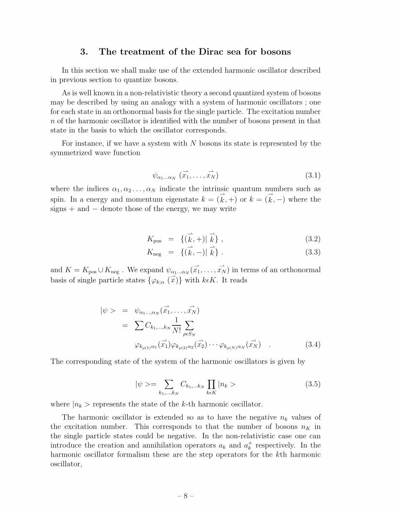
3. The treatment of the Dirac sea for bosons

In this section we shall make use of the extended harmonic oscillator describedin previous section to quantize bosons.

As is well known in a non-relativistic theory a second quantized system of bosonsmay be described by using an analogy with a system of harmonic oscillators ; onefor each state in an orthonormal basis for the single particle. The excitation numbern of the harmonic oscillator is identified with the number of bosons present in thatstate in the basis to which the oscillator corresponds.

For instance, if we have a system with N bosons its state is represented by thesymmetrized wave function

ψα1...αN(⇀x1, . . . ,

⇀xN) (3.1)

where the indices α1, α2 . . . , αN indicate the intrinsic quantum numbers such as

spin. In a energy and momentum eigenstate k = (⇀

k ,+) or k = (⇀

k,−) where thesigns + and − denote those of the energy, we may write

Kpos = {(⇀

k ,+)|⇀

k} , (3.2)

Kneg = {(⇀

k ,−)|⇀

k} . (3.3)

and K = Kpos ∪Kneg . We expand ψα1...αN(⇀x1, . . . ,

⇀xN ) in terms of an orthonormal

basis of single particle states {ϕk;α (⇀x)} with kǫK. It reads

|ψ > = ψα1...,αN(⇀x1, . . . ,

⇀xN)

=∑

Ck1,...,kN

1

N !

∑

ρǫSN

ϕkρ(1)α1(⇀x1)ϕkρ(2)α2(

⇀x2) · · ·ϕkρ(N)αN

(⇀xN ) . (3.4)

The corresponding state of the system of the harmonic oscillators is given by

|ψ >=∑

k1,...,kN

Ck1,...kN

∏

kǫK

|nk > (3.5)

where |nk > represents the state of the k-th harmonic oscillator.

The harmonic oscillator is extended so as to have the negative nk values ofthe excitation number. This corresponds to that the number of bosons nK inthe single particle states could be negative. In the non-relativistic case one canintroduce the creation and annihilation operators ak and a+k respectively. In theharmonic oscillator formalism these are the step operators for the kth harmonicoscillator,

– 8 –

a+k |nk > =√nk + 1 |nk + 1 > (3.6)

ak|nk > =√nk |nk − 1 > . (3.7)

It is also possible to introduce creation and annihilation operators for arbitrarystates |ψ >

a+(ψ) =∑

kǫK

< ϕk|ψ > a+k (3.8)

a(ψ) =∑

kǫK

ak < ϕk|ψ > , (3.9)

where the inner product is defined by∫

d3xϕ∗(x)i↔

∂ 0 ψ(x).

We then find

[a(ψ′), a+(ψ)] =∑

k,k′

< ψ′|ϕk′ > [ak′ , ak] < ϕk|ψ >

= < ψ′|ψ > . (3.10)

in which the right hand side contains an indefinite Hilbert product. Thus if weperform this naive second quantization, the possible negative norm square will beinherited into the second quantized states in the Fock space.

Suppose that we choose the basis such that for some subset Kpos the normsquare is unity

< ϕk|ϕk >= 1 for kǫKpos (3.11)

while for the complement set Kneg = K\Kpos it is

< ϕk|ϕk >= −1 for kǫKneg . (3.12)

Thus any component of a Fock space state must have negative norm square if ithas an odd number of particles in states of Kneg.

We thus have the following signs of the norm square in the naive second quan-tization

< nk|mk >= δnkmk(−1)nk (3.13)

for kǫKneg where nk and mk denote the usual nonzero levels. With use of ourextended harmonic oscillators we end up with a system of norm squared as follows:

For kǫKpos

– 9 –

< n1, n2 . . . |m1, m2, . . . >

=

δnkmkfor nk, mk = 0, 1, 2, . . .

iδnkmk(−1)nk for nk, mk = −1,−2 . . .

∞ for nk and mk in different sectors.

(3.14)

For kǫKneg

< n1, n2 . . . |m1, m2, . . . >

=

δnkmk(−1)nk for nk, mk = 0, 1, 2, . . .

iδnkmkfor nk, mk = −1,−2 . . .

∞ for nk and mk in different sectors.

(3.15)

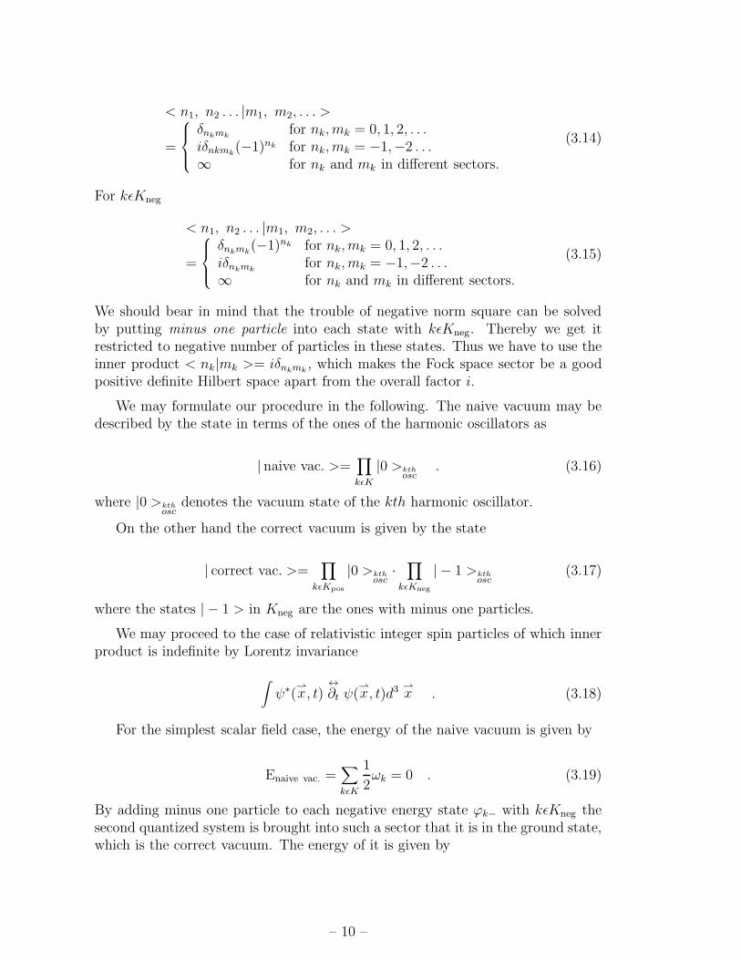
We should bear in mind that the trouble of negative norm square can be solvedby putting minus one particle into each state with kǫKneg. Thereby we get itrestricted to negative number of particles in these states. Thus we have to use theinner product < nk|mk >= iδnkmk

, which makes the Fock space sector be a goodpositive definite Hilbert space apart from the overall factor i.

We may formulate our procedure in the following. The naive vacuum may bedescribed by the state in terms of the ones of the harmonic oscillators as

| naive vac. >=∏

kǫK

|0 >kthosc

. (3.16)

where |0 >kthosc

denotes the vacuum state of the kth harmonic oscillator.

On the other hand the correct vacuum is given by the state

| correct vac. >=∏

kǫKpos

|0 >kthosc

·∏

kǫKneg

| − 1 >kthosc

(3.17)

where the states | − 1 > in Kneg are the ones with minus one particles.

We may proceed to the case of relativistic integer spin particles of which innerproduct is indefinite by Lorentz invariance

∫

ψ∗(⇀x, t)

↔

∂t ψ(⇀x, t)d3

⇀x . (3.18)

For the simplest scalar field case, the energy of the naive vacuum is given by

Enaive vac. =∑

kǫK

1

2ωk = 0 . (3.19)

By adding minus one particle to each negative energy state ϕk− with kǫKneg thesecond quantized system is brought into such a sector that it is in the ground state,which is the correct vacuum. The energy of it is given by

– 10 –

Ecorrect vac. =∑

kǫK

1

2ωk −

∑

kǫKneg

1

2ωk (3.20)

=∑

kǫK

1

2|ωk| =

∑

kǫKpos

ωk . (3.21)

It should be stressed that only inside the sector we obtain the ground state inthis way. In fact with the single particle negative energies for bosons, the totalhamiltonian may have no bottom. So if we do not add minus one particle toeach single particle negative energy state, one may find a series of states of whichenergy goes to −∞. However, by adding minus one particle we get a state of thesecond quantized system in which there is the barrier due to the laser effect. Thisbarrier keeps the system from falling back to lower energies as long as polynomialinteraction in a+k and ak are concerned.

In the above calculation for the relativistic case we have

Ecorrect vac > Enaive vac . (3.22)

Thus at the first sight the correct vacuum looks unstable. However which vacuumhas lower energy is not important for the stability of a certain proposal of vacuum.Rather the range of allowed energies for the sector of the vacuum proposal isimportant. To this end we define the energy range Erange of the vacuum by

Erange(|vac >) = {E} (3.23)

where E denotes an energy in a state which can be reached from |vac > by someoperators polynomial in a+ and a. Thus for the naive vacuum

Erange(|naive vac >) = (−∞,∞) (3.24)

while for the correct vacuum

Erange(|correct vac >) = [∑

kǫK

1

2|ωK |,∞] . (3.25)

Once the vacuum is brought into the correct vacuum state, it is no longerpossible to add particles to the state with Kneg, due to the barrier: It is ratherto subtract particles. Thus ak with kǫKneg can act on | − 1 >kth

oscwith arbitrary

number of times as

(ak)n| − 1 >kth

osc=√

|n|! | − 1− n >kthosc

. (3.26)

These subtractions we may call holes which correspond to addition of antiparticles.

It is natural to switch notations from dagger to non dagger one by defining

– 11 –

b+(−⇀

k, anti) = a(⇀

k ,−) (3.27)

and vice versa where k = (⇀

k,−) is a ω < 0 state with 3-momentum⇀

k . The

operator b+(−⇀

k, anti) denotes a creation of antiparticle with momentum⇀

k andpositive energy −ω > 0 . This is exactly the usual way of treatment of the secondquantization for bosons. The commutator of these operators reads

[b(⇀

k , anti), b+(

⇀

k′, anti)] = δ⇀k

⇀

k′. (3.28)

It should be noticed that in the boson case the antiparticles are also holes. Beforeclosing this section two important issues are discussed. The first issue is that thereare potentially possible four vacua in our approach of quantization.

We have argued that we can obtain the correct vacuum by modifying the naivevacuum so that one fermion is filled and one boson removed from each single particlenegative energy state. This opens the possibility of considering naive vacuum andassociated world of states where there exist a few extra particles. The naive vacuumshould be considered as a playground for study of the correct vacuum. It should bementioned that once we start with one of the vacua and work by filling the negativeenergy states or removing from it, we may also do so for positive energy states. Inthis way we can think of four different vacua which are illustrated symbolically astype a-d in Fig.1.

As an example let us consider the type (c) vacuum. In this vacuum the positiveenergy states are modified by filling the positive energy states by one fermion butremoving from it by one boson, while the negative energy states are not modified.Thus the single particle energy spectrum has a top but no bottom. Inversion of theconvention for the energy would not be possible to be distinguished by experimentas far as free system is concerned. However it would have negative norm squarefor all bosons and the interactions would work in an opposite manner. We shallshow in the later sections that there exists a trick of analytic continuation of thewave function to circumvent this inversion of the interaction.

Another issue to be mentioned is the CPT operation on those four vacua. TheCPT operation on the naive vacuum depicted as type (a) vacuum in Fig.1 does notget it back. The reason is that by the charge conjugation operator C all the holesin the negative energy states are, from the correct vacuum point of view, replacedby particles of corresponding positive energy states. Thus acting CPT operatoron the naive vacuum is sent into the type (c) vacuum because the positive energystates is modified while the negative ones remain the same. This fact may be statedthat in the naive vacuum CPT symmetry is spontaneously broken.

However in the subsequent paper “Dirac sea for bosons II”[1] we shall putforward another CPT-like theorem in which the CPT-like symmetry is preservedin the naive vacuum but broken in the correct one.

Before closing this section, we mention some properties of the world around thenaive vacuum where there is only a few particles. The terminology of “the worldaround a vacuum” is used for Hilbert space with a superposition of such a states

– 12 –

(c) False vacuum (d) False vacuum

(a) Naive vacuum (b) True vacuum

Figure 1: Four types of vacuaThere are four possible types of vaua for bosons as well as fermions. Here thevertical axis indicates energy level. In Figures (a) - (d) the shaded states denotethat they are all filled by one particle for fermions and minus one particle forbosons. The unshaded states are empty.

that it deviates from the vacuum in question by a finite number of particles andthat the boson does not cross the barrier. Since the naive vacuum has no particleand we can add positive number of particles which, however, can have both positiveand negative energies. The correct vacuum may similarly have a finite number ofparticles and holes in addition to the negative energy seas.

4. Wave functional formulation

In this section we develop the wave functional formulation of field theory in thenaive vacuum world.

When going over field theory in the naive field quantization

– 13 –

ϕ(⇀x, t) =

∑

⇀p ,sign

1√

|ω|a(

⇀p, sign)e−iωt+i

⇀p ·

⇀x (4.1)

π(⇀x, t) =

∑

⇀p ,sign

1√

|ω|a(

⇀p, sign) · (sign) = e−iωt+i

⇀p ·

⇀x (4.2)

we have a wave functional Ψ[ϕ]. For each eigenmode ωϕ⇀p+ iπ⇀

p, where ϕ⇀

pis

the 3-spatial Fourier transform of ϕ(x) and π⇀pis conjugate momentum, we have

an extended harmonic oscillator described in section 2. In order to see how toput the naive vacuum world into a wave functional formulation, we investigate theHamiltonian and the boundary conditions for a single particle states with a generalnorm square.

Let us imagine that we make the convention in which the n-particle state be

AnHn(x) (4.3)

with Hn the Hermite polynomial. Thus

|n >= AnHn(x)|0 > . (4.4)

On the other hand n excited state in the harmonic oscillator is given by

AnHn(x)βe− 1

2(βx)2 (4.5)

with β2 = h̄mω

. We can vary the normalization while keeping the convention

< n|n >= β−2n < 0|0 > . (4.6)

We may consider β−2 as the norm square of the single particle state correspondingto the harmonic oscillator.

Now the Hamiltonian of the harmonic oscillator is expressed in terms of ω andβ−2 as follows:

H = − ω

2 < s.p|s.p >d2

dx2+

1

2< s.p|s.p > ωx2 (4.7)

where |s.p > denotes the single particle state and thus

< s.p|s.p >= mω = β−2 (4.8)

with h̄ = 1. Therefore we obtain the Hamiltonian

H = −1

2β2ω

d2

dx2+

1

2β−2ωx2 (4.9)

– 14 –

Remark that if one wants < s.p|s.p > negative for negative ω one, β turns out

to be pure imaginary. Thus e−12(βχ)2 blows up so that the wave functions become

like the one in the extended negative sector discussed in the previous sections.

By passing to the correct vacuum world by removing one particle from eachnegative energy state, the boundary conditions for the wave functional are changedso as to converge along the real axis for all the modes. Remember they are alongthe imaginary axis for the negative energy modes in the naive vacuum.

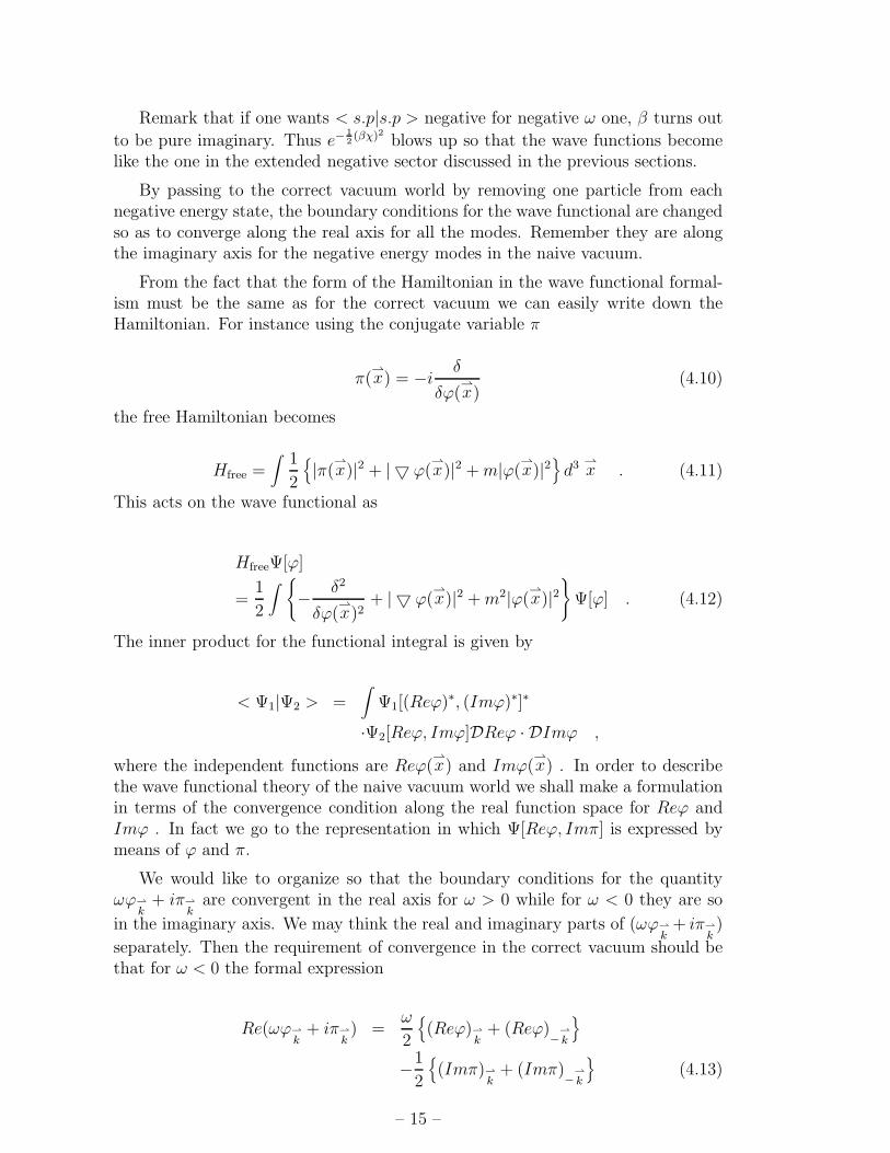
From the fact that the form of the Hamiltonian in the wave functional formal-ism must be the same as for the correct vacuum we can easily write down theHamiltonian. For instance using the conjugate variable π

π(⇀x) = −i δ

δϕ(⇀x)

(4.10)

the free Hamiltonian becomes

Hfree =∫

1

2

{

|π(⇀x)|2 + | ▽ ϕ(⇀x)|2 +m|ϕ(⇀x)|2

}

d3⇀x . (4.11)

This acts on the wave functional as

HfreeΨ[ϕ]

=1

2

∫

{

− δ2

δϕ(⇀x)2

+ | ▽ ϕ(⇀x)|2 +m2|ϕ(⇀x)|2

}

Ψ[ϕ] . (4.12)

The inner product for the functional integral is given by

< Ψ1|Ψ2 > =∫

Ψ1[(Reϕ)∗, (Imϕ)∗]∗

·Ψ2[Reϕ, Imϕ]DReϕ · DImϕ ,

where the independent functions are Reϕ(⇀x) and Imϕ(

⇀x) . In order to describe

the wave functional theory of the naive vacuum world we shall make a formulationin terms of the convergence condition along the real function space for Reϕ andImϕ . In fact we go to the representation in which Ψ[Reϕ, Imπ] is expressed bymeans of ϕ and π.

We would like to organize so that the boundary conditions for the quantityωϕ⇀

k+ iπ⇀

kare convergent in the real axis for ω > 0 while for ω < 0 they are so

in the imaginary axis. We may think the real and imaginary parts of (ωϕ⇀

k+ iπ⇀

k)

separately. Then the requirement of convergence in the correct vacuum should bethat for ω < 0 the formal expression

Re(ωϕ⇀

k+ iπ⇀

k) =

ω

2

{

(Reϕ)⇀k+ (Reϕ)

−⇀

k

}

−1

2

{

(Imπ)⇀k+ (Imπ)

−⇀

k

}

(4.13)

– 15 –

and

Im(ωϕ⇀

k+ iπ⇀

k) =

ω

2

{

(Imϕ)⇀k+ (Imϕ)

−⇀

k

}

+1

2

{

(Reπ)⇀k+ (Reπ)

−⇀

k

}

(4.14)

are purely imaginary along the integration path for which the convergence is re-quired.

We may use the following parameterization in terms of the two real functionsχ1 and χ2 :

Reϕ = −(1 + i)χ1 − (1− i)χ2

Imπ = (1− i)χ1 + (1 + i)χ2

By this parameterization the phases of ωϕ⇀

k+ iπ⇀

klay in the intervals

]− π

4,π

4[ for ω > 0

and

]π

4,3π

4[ for ω < 0

modulo π. They provide the boundary conditions for the naive vacuum world whenconvergence of Dχ1Dχ2 integration is required.

In this way we find the naive vacuum world with usual wave functional hamil-tonian operator. However, we do not require the usual convergence condition

∫

Ψ(Reϕ, Imϕ)∗Ψ(Reϕ, Imϕ)DReϕDImϕ <∞ (4.15)

but instead require

< Ψ|Ψ >=∫

Ψ[(Reϕ)∗, (Imπ)∗]∗Ψ[Reϕ, Imϕ]Dχ1Dχ2 <∞ (4.16)

where the left hand side is defined along the path with χ-parameterization. Theinner product corresponding to this functional contour is

< Ψ1|Ψ2 > =∫

Ψ1[−(1− i)χ1 − (1 + i)χ2, (1 + i)χ1 + (1− i)χ2]∗

Ψ2[−(1 + i)χ1 − (1− i)χ2, (1− i)χ1 + (1 + i)χ2]Dχ1Dχ2 .(4.17)

This is not positive definite, and that is related to the fact that there are lot ofnegative norm square states in the Fock space in the naive vacuum world.

The method of filling the Dirac sea vacuum for fermions is now extended tothe case of bosons that first in the naive vacuum we have the strange convergencecondition eq.(4.15). We then go to the correct vacuum by switching the boundaryconditions to the convergence ones along the real axis e.g. Reϕ and Imπ real.

– 16 –

5. Double harmonic oscillator

To illustrate how our functional formalism works we consider as a simple ex-ample a double harmonic oscillator. It is relevant for us in the following threereasons:

1) It is the subsystem of field theory which consists of two single particle states

with pµ = (⇀p, ω(

⇀p)) and −pµ = (− ⇀

p,−ω(⇀p)) for ω(⇀p) > 0 .

2) It could correspond a single 3-position field where the gradient interaction isignored.

3) It is a 0 + 1 dimensional field theory model.

We start by describing the spectrum for free case corresponding to a two statesystem in which the two states have opposite ω’s. The boundary conditions in thenaive vacuum world is given by

∫

ψ ((Reϕ)∗ , (ImΠ)∗)∗ψ (Reϕ, ImΠ) dχ1χ2

=∫

ψ (− (1− i)χ1 − (1 + i)χ2, (1 + i)χ1 + (1− i)χ2)∗

· ψ (− (1 + i)χ1 − (1− i)χ2, (1− i)χ1 + (1 + i)χ2) dχ1dχ2 <∞ (5.1)

which is similar to eq.(4.17). However in eq.(5.1) the quantities χ1 and χ2 are notfunctions, but just real variables. Here we use a mixed representation in terms ofposition variables Reϕ and Imϕ and conjugate momenta

Reπ = −i ∂

∂Reϕ, Imπ = −i ∂

∂Imϕ(5.2)

The Hamiltonian may be given by a rotationally symmetric 2 dimensional oscil-lator because the two ω’s are just opposite. From eq.(4.7) the coefficient of ∂2

∂Imϕ2

is

−ω2 < s.p|s.p. > (5.3)

and that of (Imϕ)2 is

1

2< s.p.|s.p. > ω (5.4)

where |s.p > denotes the single particle state. These coefficients are the same forboth oscillators and thus the Hamiltonian reads

– 17 –

H = −1

2|ω| ∂

∂ϕ

∂

∂ϕ∗+

1

2|ω|ϕ∗ϕ

=1

2|ω|

(

− ∂2

∂Reϕ2− ∂2

∂Imϕ2+Reϕ2 + Imϕ2

)

.

which is expressed in the mixed representation as

H =1

2|ω|

(

− ∂2

∂Reϕ2+Reϕ2 + Imπ2 − ∂2

∂Imπ2

)

. (5.5)

We may express H in terms of the real parameterization χ1 and χ2 by using therelations

Reϕ = −(1 + i)χ1 − (1− i)χ2

Imπ = (1− i)χ1 + (1 + i)χ2 .

It may be convenient to define

χ± =√2(χ2 ± χ1) (5.6)

so that the Hamiltonian can be simply expressed

H =1

2|ω|

(

∂2

∂χ2−

− χ2− − ∂2

∂χ2+

+ χ2+

)

. (5.7)

The inner product takes the form

< ψ̃1|ψ̃2 >=∫

ψ̃1(−χ−, χ+)∗ψ̃2(χ−, χ+)dχ−dχ+ (5.8)

where

ψ̃i(χ−, χ−) = ψi(−√2χ+ + i

√2χ−,

√2χ+ + i

√2χ−) (5.9)

As to be expected the Hamiltonian turns out to be two uncoupled harmonicoscillators expressed in terms of χ−and χ+. The χ+ oscillator is usual one whileχ− has the following two deviations : one is that it has over all negative sign.The other one is that in the definition of the inner product −χ− instead of χ− isused in the bra wave function. This is equivalent to abandoning a parity operationχ− → −χ− in the inner product.

The energy spectrum is made up from all combinations of a positive contribu-tion |ω|(n+ + 1

2) with a negative one −|ω|(n− + 1

2) so that

E = |ω|(n+ − n−) . (5.10)

– 18 –

The norm square of these combination of the eigenstates are (−1)n−−1 which equalsto the parity under the χ− parity operation χ− → −χ− .

If we consider the single particle state, the charge or the number of particles isgiven by

Q =i

4

{

π+, ϕ}

− i

4

{

ϕ+, π}

=1

2χ2+ − 1

2

∂2

∂χ2+

+1

2χ2− − 1

2

∂2

∂χ2−

− 1 . (5.11)

This is simply a sum of two harmonic oscillator Hamiltonians with the same unitfrequency. Thus the eigenvalue Q′ of Q can only take positive integer or zero. Fora given value Q′ that is number of particle in either of the two states, the energycan vary from E = −|ω|Q′ to E = |ω|Q′ in integer steps in 2|ω| . Thus we can put

n− = Q′, Q′ − 1, Q′ − 2, · · · , 0 (5.12)

in the negative ω states while in the positive energy state we have

n+ = Q− n− . (5.13)

So the energy eq.(5.10) can be written as

E = |ω|(Q− 2n−) (5.14)

which is illustrated in Fig.2(a). By going to the convergence condition along thereal axis we get the usual theory with correct vacuum, see Fig.2(b).

The wave function of the naive vacuum is given by

ψn.υ. = N exp(

−1

2χ2− − 1

2χ2+

)

(5.15)

with a normalization constant N . We may transform eq.(5.14) in the mixed trans-formation back to the position representation by Fourier transformation

ψn.υ.(Reϕ, Imϕ) =∫

eiImΠ·Imϕψn.υ(Reϕ, ImΠ)dImΠ

= N∫

eiImΠ·ImϕeImΠ·ReϕdImΠ .

= Nδ(Imϕ− iReϕ) . (5.16)

Here δ-function is considered as a functional linear in test functions that are ana-lytic and goes down faster than any power in real directions and no faster than acertain exponential in imaginary direction. This function may be called the distri-bution class Z ′ according to Gel’fand and Shilov [7]. Thus our naive vacuum wavefunction is δ-function that belongs to Z ′.

– 19 –

✻

✲

E

Qt

t

t

t

t

t

t

❤t

t

t

3

3

✻

✲

E

Qt

t

t

t

t

t

t

❤t

tt33

(a) Naive vacuum (b) True vacuum

Figure 2: charge vs energy in two state systemEnergy E versus charge Q=number of particles in the two state system describedin the text. This two state system is really a massive boson theory in 1 time+0space dimensions. The single dot · indicates that there is only one Fock space statewhile the symbol

⊙

means that there are two Fock space states with the quantumnumber E and Q. The single dot with 3 is that there are 3 states and so on. Thetriangles of dots are to be understood to extend to infinity. The naive vacuum isdepicted in Figure (a), while Figure (b) is for the case of the true vacuum.

By acting polynomials in creation and annihilation operators to the naive vac-uum state we obtain the expression of the form

∑

n,m=0,1,...

an,m(Reϕ− iImϕ)nδ(m)(Reϕ+ Imϕ) . (5.17)

Thus the wave functions of the double harmonic oscillator in the naive vacuumworld are composed of eq.(5.17).

As long as the charge Q is kept conserved, even an interaction term such asan anharmonic double oscillator with phase rotation symmetry, only the states ofthe form eq.(5.17) can mix each other. For such a finite quantum number Q thereis only a finite number of these states of the form. Therefore even to solve theanharmonic oscillator problem would be reduced to finite matrix diagonalization.In this sense the naive vacuum world is more easier to solve than the correct vacuumworld.

To higher dimensions we may extend our result of the double harmonic oscillatorfor the naive vacuum. The naive vacuum world would involve polynomials in the

– 20 –

combinations that are not present in the δ-functionals and their derivatives.

6. The Naive vacuum world

In this section we shall investigate properties of the naive vacuum world. Itis obvious that this world has the following five inappropriate properties from thepoint of view of phenomenological applications:

1) There is no bottom in the energy.

2) The Hilbert space is not a true Hilbert space because it is not positive definite.The states with an odd number of negative energy bosons get an extra minussign in the norm square.

We may introduce the boundary conditions to make a model complete whichmay be different for negative energy states. As will be shown in the followingpaper “Dirac Sear for Bosons II”[1] in order to make an elegant CPT-likesymmetry we shall propose to take the boundary condition for the negativeenergy states such that bound state wave functions blow up.

3) We cannot incorporate particles which are their own antiparticles. Thus weshould think that all particles have some charges.

4) The naive vacuum world can be viewed as a quantum mechanical systemrather than second quantized field theory. It is so because we think of afinite number of particles and the second quantized naive vacuum world is ina superposition of various finite numbers of particles.

5) As long as we accept the negative norm square there is no reason for quantiz-ing integer spin particles as bosons and half integer ones as fermions. Indeedwe may find the various possibilities as is shown in table 1. In this tablewe recognize that the wellknown spin-statistics theorem is valid only underthe requirement that the Hilbert space is positive definite. It should be no-ticed that in the naive vacuum world with integer spin states negative normsquares exist anyway and so there is no spin-statistics theorem. When wego to the correct vacuum it becomes possible to avoid negative norm square.Then this calamity of indefinite Hilbert space is indeed avoided by choosingthe Bose or Fermi statistics according to the spin-statistics theorem which isdepicted in table 2.

7. Conclusions

We have put forward an attempt to extend also to bosons the idea of Dirac seafor fermions. We first consider one second quantization called the naive vacuum

– 21 –

❳❳❳❳❳❳❳❳❳❳❳❳statisticsspin

S = 12, 32, . . . S = 0, 1, . . .

Fermi-Dirac ‖ · · · ‖2 ≥ 0 IndefiniteBose-Einstein ‖ · · · ‖2 ≥ 0 Indefinite

Table 1: Spin-statistics theorem for naive vacuum

❳❳❳❳❳❳❳❳❳❳❳❳statisticsspin

S = 12, 32, . . . S = 0, 1, . . .

Fermi-Dirac ‖ · · · ‖2 ≥ 0 IndefiniteBose-Einstein Indefinite ‖ · · · ‖2 ≥ 0

Table 2: Spin-statistics theorem for true vacuum

world in which there exist a few positive and negative energy fermions and bosonsbut no Dirac sea for fermions as well as bosons yet. This first picture of thenaive vacuum world model is very bad with respect to physical properties in asfar as no bottom in the Hamiltonian. For bosons this naive vacuum is even worsephysically because in addition to negative energies without bottom a state withan odd number of negative energy bosons has negative norm square. There is noreal Hilbert space but only an indefinite one. At this first step of the bosons theinner product for the Fock space is not positive definite. Thus this first step iscompletely out from the phenomenological point of view for the bosons as well asfor the fermions. For the bosons there are for two major reasons : negative energyand negative norm square.

However, from the point of view of theoretical study this naive vacuum world atthe first step is very attractive because the treatment of a few particles is quantummechanics rather than quantum field theory. Furthermore by locality the systemof several particles becomes free in the neighborhood of almost all configurationsexcept for the case that some particles meet and interact. We encourage the use ofthis theoretically attractive first stage as a theoretical playground to gain physicalunderstanding of the real world, the second stage.

In the present article we studied the naive vacuum world at first stage. Wewould like to stress the major results in the following :

1) In the naive vacuum the single particles can be in position eigenstates con-trary to the particles in the “true” relativistic theories.

2) The Fock space for the bosons is an indefinite one.

3) The bottom of the Hamiltonian is lost. We made some detailed calculationson this issue.

– 22 –

4) We found the main feature of the wave functionals for the bosons. They arederivatives of δ-functionals of the complex field multiplied by polynomials inthe complex conjugate of the field. These singular wave functionals form aclosed class when acted upon by polynomials in creation and annihilation op-erators. Especially we worked through the case of one pair of a single particlestate with a certain momentum and the one with the opposite momentum.

5) In a subsequent “Dirac Sea for Bosons II” paper we will present a CPT-likesymmetry. A reduced form of strong reflection provides an extra transforma-tion that is an analytic continuation of the wave function onto another sheetamong 2

12N(N+1) ones for the wave function of the N particle system. The

sheet structure occurs because rik is a square root so that it has 2 sheets.For each of the 1

2N(N + 1) pairs of particles there is a dichotomic choice of

sheet so that it gives 212N(N+1) sheets.

The main point of our present work was to formulate the transition from thenaive vacuum of the first stage into the next stage of the correct vacuum. Forfermions it is known to be done by filling the negative energy states which isnothing but filling up the Dirac sea. The corresponding procedure to bosons turnsout to be that from each negative energy single particle states one boson is removed,that is minus one boson is added. This removal cannot be done quite as physicallyas the adding of a fermion, because there is a barrier to be crossed.

We studied this by using the harmonic oscillator corresponding to a singleparticle boson state. We replaced the usual Hilbert norm requirement of finitenessby the requirement of analyticity of the wave function in the whole complex x-plane except for x = ±∞. The spectrum of this extended harmonic oscillatoror the harmonic oscillator with analytic wave function has an additional series oflevels with negative energy in addition to the usual one. The wave functions withnegative energy are of the form with Hermite polynomials times e

12(βx)2 .

We note that there is a barrier between the usual states and the one withnegative excitation number because annihilation or creation operators cannot crossthe gap between these two sectors of states. The removal of one particle from anempty negative energy state implies crossing the barrier. Although it cannot bedone by a finite number of interactions expressed as a polynomial in creation andannihilation operators we may still think of doing that. Precisely because of thebarrier it is allowed to imagine the possibilities that negative particle numberscould exist without contradicting with experiment.

Once the barrier has been passed to the negative single particle states in aformal way the model is locked in and those particles cannot return to the positivestates. Therefore it is not serious that the correct vacuum for bosons get a higher

energy than the states with a positive or zero number of particles in the negativeenergy ones.

Finally we mention that our deep motivation why we come to study in detailalready established standard 2nd quantization procedure in a different point ofview presented in this paper. As was mentioned in the introduction once we come

– 23 –

to the quantization of the string theories we may face problem even in the 1stquantization unless we use the light-cone gauge which was pointed out long ago[8] by Jackiw et al. Furthermore there does not seem to exist satisfactory stringfield theories except for Kaku-Kikkawa’s light-cone string field theories. We expectthat our bosonic quantization procedure may clarify these problem in the stringtheories.

Acknowledgment

We would like to thank J. Greensite for useful discussions on string field theories.We also acknowledge R. Jackiw for telling us the ref [7]. Main part of this researchwas performed at YITP while one of us (H.B.N.) stayed there as a visiting professor.H.B.N. is grateful to YITP for hospitality during his stay. M.N. acknowledges N.B.Ifor hospitality extended to him during his visit. This work is partially supportedby Grants-in-Aid for Scientific Research on Priority Areas, Number of Areas 763,“Dynamics of Strings and Fields”, from the Ministry of Education of Culture,Sports, Science and Technology, Japan.

References

[1] H.B. Nielsen and M. Ninomiya, “Dirac Sea for Bosons II – Study of the NaiveVacuum Theory for the Playground World prior to Filling the Negative EnergySea –”, Oct.2004, hep-th/0410218

[2] H.B. Nielsen and M. Ninomiya, Los Alamos arxive, hep-th9808108, Aug.1998.

[3] P.A.M. Dirac, Proc. Roy. Soc. A126 (1930) 360 ; Proc. Cambridge Phil. Soc.26 (1930) 376.

[4] S, Weinberg, “The Quantum Theory of Fields; Vol.I, Foundations” 12-14(Cambridge University Press, 1995).

[5] J.J. Sakurai, “ Invariance Principles and Elementary Particles”, (PrincetonUniversity Press, Princeton, New Jersey, 1964).

[6] M. Kaku and K. Kikkawa, Phys. Rev.D10 (1974) 1110-1133 ; ibid, 1823-1843.

[7] I.M. Gel’fand and G.E Shilov, “Generalized Functions Vol.I”, (AcademicPress, New York and London, 1964).

[8] E. Benedict, R. Jackiw and H-J. Lee, Phys. Rev. D54 (1996) 6213-6225.

– 24 –