Embed Size (px)
Citation preview
Dipole trapping andmanipulation of ultra-cold
atoms
Andrian Harsono
A thesis submitted in partial fulfilment ofthe requirements for the degree of
Doctor of Philosophy at the University of Oxford
Merton CollegeUniversity of Oxford
Trinity Term 2006
Abstract
Dipole trapping and manipulation of ultra-coldatoms
Andrian Harsono, Merton College, Oxford UniversityDPhil Thesis, Trinity Term 2006
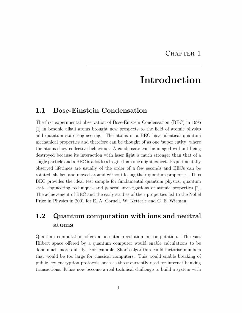
A large part of this thesis describes the construction of a new Bose-Einstein Con-densation (BEC) experiment starting in October 2003. The magnetic trap setupthat was used was a baseball trap accompanied by two pairs of compensation coils(primary and secondary). This setup is capable of producing a magnetic trap ofradial trapping frequency of 178.6 Hz and an axial trapping frequency of 5.7 Hz.After an evaporative cooling sequence lasting 85 seconds, we observed phase tran-sition to BEC at 6.5 × 10⁵ atoms at temperature of 320 nK and when the thermalcomponent of our cloud of atoms almost vanished completely, we had 1.5 × 10⁵
atoms at BEC with our thermal component at a temperature of 120 nK.
The objective of all subsequent experiments beyond BEC was to investigate andunderstand the manipulation of ultra-cold atoms in dipole traps. An Acousto-Optic Deflector (AOD) capable of light diffraction in the X and Y axes was usedto manipulate our dipole trap and it has been demonstrated that this experimentcould split a dipole trap into two separate traps the separation between whichcould be varied by varying the frequency of the signal input into the AOD. Whenatoms in a single dipole trap were first observed, there were about 7000 atoms inthe trap and at this moment the experiment is capable of producing this number ofatoms in our dipole trap quite reproducibly. Then, the thesis describes a successfulbasic demonstration of the generation of a simple 2 × 2 array of 2-dimensionaloptical lattice. When such an array was first produced, the separation betweenneighbouring lattice sites was 30 µm.
In addition, the thesis describes an investigation into the fluorescence imagingsetup used to observe the above phenomena. The magnification of such a systemwas estimated to be 24. A probing sequence was then decided which would produceas much signal as possible from the atoms without heating them by too great anamount. With this probing sequence, an experiment was carried out to gaugehow small an atom number this imaging system could detect and this numberwas around 500 atoms. With further improvements, we hope for the fluorescenceimaging system to detect single atoms.
i

Acknowledgements
Building this experiment had not been an easy task, but there are those who
worked with me who made the experience somewhat less painful and this section
is dedicated to them without whom this thesis would never happen.
I want to thank my supervisor Prof. Christopher Foot for his guidance, support
and encouragement along the way. I also want to thank the two post-docs in my
life, Simon Cornish and Gerald Hechenblaikner who helped shape me to be the
scientist that I am.
My eternal gratitude goes to the people in -111 who helped me set up the exper-
iment as it stands: Martin Shotter, Ben Fletcher, Min Sung Yoon, C M Chan-
drashekar, James Zacks, Peter Baranowski and Gerald Hechenblaikner. Their
contribution towards the experiment had been vital and absolutely priceless. My
thanks also to other members of the group who had helped me out in one way or
another whenever I was in serious trouble: Rachel Godun, Giuseppe Smirne, Ma
Zhao Yuan, William Heathcote, Eileen Nugent, , Benjamin Sheard, Amita Deb
and Vincent Boyer.
And what about other members of staff? I want to say a big thank you as well to
the technicians I have worked with: Graham Quelch, George Matthews and the
champion of them all, Rob Harris. There were also other people outside physics
who have helped me overcome the occasional stress and gave me the best years of
my life at Oxford, my friends at Merton College and in London and overseas.
Finally, to my parents and brothers for their love and support, who stood by my
decision to do physics despite being born in a family of businessmen. My mother
may not know this, but I do get homesick even though I rarely call home...
ii

Contents
1 Introduction 1
1.1 Bose-Einstein Condensation . . . . . . . . . . . . . . . . . . . . . . 1
1.2 Quantum computation with ions and neutral atoms . . . . . . . . . 1
1.3 Quantum bit register . . . . . . . . . . . . . . . . . . . . . . . . . . 3
1.4 Experimental proposal . . . . . . . . . . . . . . . . . . . . . . . . . 3
1.5 Abbreviations used in thesis . . . . . . . . . . . . . . . . . . . . . . 4
2 Theory of BEC and experimental techniques 6
2.1 Experimental aspects of BEC . . . . . . . . . . . . . . . . . . . . . 6
2.1.1 Atomic properties of Rubidium-87 . . . . . . . . . . . . . . . 6
2.1.2 The ideal Bose gas . . . . . . . . . . . . . . . . . . . . . . . 8
2.2 Laser cooling . . . . . . . . . . . . . . . . . . . . . . . . . . . . . . 15
2.2.1 Doppler cooling . . . . . . . . . . . . . . . . . . . . . . . . . 16
2.2.2 Sub-Doppler cooling . . . . . . . . . . . . . . . . . . . . . . 17
2.3 Magneto-optical traps . . . . . . . . . . . . . . . . . . . . . . . . . 21
2.3.1 Six-beam MOT . . . . . . . . . . . . . . . . . . . . . . . . . 22
2.3.2 Pyramidal MOT . . . . . . . . . . . . . . . . . . . . . . . . 23
2.4 Magnetic trapping of neutral atoms . . . . . . . . . . . . . . . . . . 23
2.4.1 Zeeman effect on the hyperfine ground states . . . . . . . . . 25
2.4.2 The Ioffe-Pritchard trap . . . . . . . . . . . . . . . . . . . . 27
2.5 Evaporative cooling . . . . . . . . . . . . . . . . . . . . . . . . . . . 29
2.5.1 Evaporative cooling . . . . . . . . . . . . . . . . . . . . . . . 30
2.5.2 RF-evaporative cooling . . . . . . . . . . . . . . . . . . . . . 32
2.6 Sub-shot noise measurements of atom number . . . . . . . . . . . . 33
2.6.1 Dipole trapping of neutral atoms . . . . . . . . . . . . . . . 33
2.6.2 The Mott Insulator State . . . . . . . . . . . . . . . . . . . . 37
3 The Experimental Apparatus 40
3.1 The BEC Apparatus . . . . . . . . . . . . . . . . . . . . . . . . . . 40
iii

CONTENTS iv
3.1.1 Lasers . . . . . . . . . . . . . . . . . . . . . . . . . . . . . . 40
3.1.2 The optical table . . . . . . . . . . . . . . . . . . . . . . . . 41
3.1.3 Frequency stabilization . . . . . . . . . . . . . . . . . . . . . 45
3.1.4 Vacuum system . . . . . . . . . . . . . . . . . . . . . . . . . 49
3.1.5 Pyramidal MOT . . . . . . . . . . . . . . . . . . . . . . . . 50
3.1.6 2nd MOT - experimental MOT . . . . . . . . . . . . . . . . 53
3.1.7 Magnetic trap . . . . . . . . . . . . . . . . . . . . . . . . . . 56
3.1.8 Evaporation . . . . . . . . . . . . . . . . . . . . . . . . . . . 63
3.2 Dipole trap apparatus . . . . . . . . . . . . . . . . . . . . . . . . . 63
3.2.1 Lasers . . . . . . . . . . . . . . . . . . . . . . . . . . . . . . 64
3.2.2 Acousto-Optic Deflector . . . . . . . . . . . . . . . . . . . . 65
3.2.3 CCD Camera . . . . . . . . . . . . . . . . . . . . . . . . . . 69
3.2.4 Four-lens objective . . . . . . . . . . . . . . . . . . . . . . . 70
3.3 Diagnostics . . . . . . . . . . . . . . . . . . . . . . . . . . . . . . . 72
3.3.1 Recapture method . . . . . . . . . . . . . . . . . . . . . . . 72
3.3.2 Absorption imaging . . . . . . . . . . . . . . . . . . . . . . . 73
3.3.3 Image analysis . . . . . . . . . . . . . . . . . . . . . . . . . . 79
4 Producing BEC 82
4.1 Loading the magnetic trap . . . . . . . . . . . . . . . . . . . . . . . 82
4.1.1 Pyramidal MOT . . . . . . . . . . . . . . . . . . . . . . . . 84
4.1.2 Experimental MOT . . . . . . . . . . . . . . . . . . . . . . . 84
4.1.3 Compressed MOT and optical molasses . . . . . . . . . . . . 87
4.1.4 Optical pumping . . . . . . . . . . . . . . . . . . . . . . . . 91
4.2 Magnetic trapping . . . . . . . . . . . . . . . . . . . . . . . . . . . 92
4.2.1 Measurement of trapping frequencies . . . . . . . . . . . . . 92
4.2.2 Adiabatic compression and the tight Ioffe trap . . . . . . . . 94
4.3 Evaporative cooling . . . . . . . . . . . . . . . . . . . . . . . . . . . 96
4.3.1 Evaporation stages . . . . . . . . . . . . . . . . . . . . . . . 96
4.3.2 Observation of Bose-Einstein Condensation . . . . . . . . . . 99
5 Dipole trapping and manipulation of ultra-cold atoms 102
5.1 Characterisation of the fluorescence imaging system . . . . . . . . . 102
5.1.1 Initial dipole trapping . . . . . . . . . . . . . . . . . . . . . 102
5.1.2 Positioning the four-lens objective . . . . . . . . . . . . . . . 107
5.1.3 Some estimates of fluorescence imaging parameters . . . . . 109
5.1.4 Generation and manipulation of multiple spots . . . . . . . . 109
5.2 Characterisation of the dipole traps . . . . . . . . . . . . . . . . . . 110
5.2.1 Beam waist measurement . . . . . . . . . . . . . . . . . . . 110

CONTENTS v
5.2.2 Loss rate of atoms in the dipole trap . . . . . . . . . . . . . 113
5.2.3 Probing sequence . . . . . . . . . . . . . . . . . . . . . . . . 115
5.2.4 Low atom number detection . . . . . . . . . . . . . . . . . . 117
5.2.5 Generation and manipulation of multiple dipole traps . . . . 119
6 Conclusion and future work 123
6.1 Achievements so far . . . . . . . . . . . . . . . . . . . . . . . . . . . 123
6.2 Future work . . . . . . . . . . . . . . . . . . . . . . . . . . . . . . . 124
6.2.1 Adiabatic loading of BEC . . . . . . . . . . . . . . . . . . . 124
6.2.2 Imaging and single atom detection . . . . . . . . . . . . . . 125
6.2.3 2D optical lattice and the Mott Insulator state . . . . . . . . 125
Appendices 127
A Rubidium-87 data 127
B Beam waist measurement 128
C Calculating atom number from a Magneto-Optical trap 130
D Signal to noise ratio between absorption and fluorescence imaging132
E Control 135
Chapter 1
Introduction
1.1 Bose-Einstein Condensation
The first experimental observation of Bose-Einstein Condensation (BEC) in 1995
[1] in bosonic alkali atoms brought new prospects to the field of atomic physics
and quantum state engineering. The atoms in a BEC have identical quantum
mechanical properties and therefore can be thought of as one ‘super entity’ where
the atoms show collective behaviour. A condensate can be imaged without being
destroyed because its interaction with laser light is much stronger than that of a
single particle and a BEC is a lot less fragile than one might expect. Experimentally
observed lifetimes are usually of the order of a few seconds and BECs can be
rotated, shaken and moved around without losing their quantum properties. Thus
BEC provides the ideal test sample for fundamental quantum physics, quantum
state engineering techniques and general investigations of atomic properties [2].
The achievement of BEC and the early studies of their properties led to the Nobel
Prize in Physics in 2001 for E. A. Cornell, W. Ketterle and C. E. Wieman.
1.2 Quantum computation with ions and neutral
atoms
Quantum computation offers a potential revolution in computation. The vast
Hilbert space offered by a quantum computer would enable calculations to be
done much more quickly. For example, Shor’s algorithm could factorise numbers
that would be too large for classical computers. This would enable breaking of
public key encryption protocols, such as those currently used for internet banking
transactions. It has now become a real technical challenge to build a system with
1
1.2. Quantum computation with ions and neutral atoms 2
extremely good isolation against environmental decoherence and where interactions
between quantum bits can be turned on and off on demand.
Enormous progress has been made in atomic, molecular and optical physics in
controlling the quantum states of atoms and photons and suppressing decoherence
due to unwanted interactions with the environment. Nowadays it is possible to
engineer quantum states and also create and manipulate entanglement between
atoms as a resource as suggested by quantum information theory. Once control
techniques over atoms, photons and ions are mastered, the next milestone would be
to bring together these fundamental elements and use them to build more complex
systems with applications in quantum information processing.
Two systems that have made large steps towards quantum computation are trapped
ions [3] [4] [5] and cold atoms in optical lattices [6] [7] [8]. Experiments with trapped
ions have focused on control at the single ion level. These setups are used for the
creation of entanglement, precision measurements and small-scale quantum com-
putations and are currently the most promising candidate for quantum computing.
On the other hand, experiments with neutral atoms provide us with systems with
a large number of subsystems, particles or quantum bits (qubits). In addition, an
advantage that neutral atoms have over ions in quantum computation experiments
is scalability. Atomic qubits have properties similar to ionic qubits, but whereas
the position and state of one ionic qubit can affect all qubits due to the long-range
Coulomb interaction, atomic qubits are uncoupled from each other unless in direct
contact. At close proximity, the short-range collisional interactions may be used
to entangle atomic qubits. Two other types of experiments where quantum gates
have been implemented but suffer from potential scalability problems are NMR [9]
and within a quantum dot [10].
There is potential for cold atoms in optical lattices to perform quantum gates in a
parallel way and cold atoms are also suited for other applications such as quantum
simulation of systems in condensed matter physics and the creation of entangled
states of many particles. Currently, these experiments typically lack addressability
i.e. it is difficult to prepare the basic unit, the atomic qubit, which is defined as a
single atom in the ground state of a single well which can be manipulated. What
has been demonstrated so far is many atoms in the ground state of many wells [8]
with about one atom per well but not individual addressability, and a single atom
in a single well, but not in the ground state of this well [11].
A useful review article discussing current progress in quantum information pro-
cessing with ions and cold atoms can be found in [12].
1.3. Quantum bit register 3
1.3 Quantum bit register
An integral part of quantum computation is the ability to create a qubit register. A
possible physical system that serves this purpose is an array of microtraps for cold
atoms in the form of an optical lattice. As first proposed [6] [7], a large number of
ultra-cold atoms can be loaded from a BEC into an optical lattice which is nothing
more than a standing wave of light that confines the atoms at points of either the
maxima or the minima of light intensities. In very strong confinement, the system
behaves as a Mott Insulator where it consists of one atom per lattice site. When
the internal states of these atoms are used as qubits, they can be entangled in
a parallel operation with spin-dependent confinement [13]. This thesis describes
work aiming to establish such a register where qubit operations can be carried out
and the next section will describe how this particular experiment is different from
most other experiments involving optical lattices.
1.4 Experimental proposal
This section describes the proposed experiments in Oxford. The first stage has been
to achieve BEC by standard techniques that have been understood, studied and
perfected over the years such as magnetic trapping of neutral atoms with a Ioffe-
Pritchard trap, laser-cooling with a Magneto-Optical Trap (MOT), evaporative
cooling and absorption imaging.
The next stage is dipole trapping. We have loaded atoms from our cloud of ultra-
cold atoms into a red-detuned dipole trap and we wish to manipulate the atoms in
the dipole trap with the help of an acousto-optic deflector (AOD). Sending multiple
frequency inputs into the AOD generates multiple laser beam spots and therefore
multiple dipole traps. These traps can be manipulated and moved independently
and in real-time to provide the addressability of the atoms missing in other ultra-
cold matter experiments with optical lattices. We have also built a fluorescence
imaging setup with a diffraction limited objective lens that should be capable of
single-atom detection although this has not yet been demonstrated. A large step
forward would then be to establish a number-squeezed state of the atom cloud that
we have. This is achieved by suppressing the tunnelling of atoms between lattice
sites either by raising the potential barrier between the sites [8] or by moving the
sites further apart.
This highly-entangled system would provide the foundation for qubit operations.
Initially, the experiment must be capable of the deterministic preparation of atomic
qubits. This means preparing a single atom on demand in the lowest energy state
1.5. Abbreviations used in thesis 4
of an energy well. If we could control the number of atoms in the mini-lattice of
laser beam spots, we could also control the average occupancy of each well. To
evenly distribute the atom number over the lattice we could enter the Mott regime
by adiabatically increasing the distance between each well, and this should produce
a lattice with the majority of the sites having one atom per well. In the near future,
we may try encoding single qubits, for example with schemes involving hyperfine
levels or in the spatially delocalised qubit scheme [14] which involves bringing wells
together, and apart, adiabatically and reproducibly. Also, we could try 2 qubit
operations, the simplest of which would be cold controlled collisions between two
atoms [7].
1.5 Abbreviations used in thesis
Many abbreviations will be used throughout the thesis. The first time these are
used, they will be accompanied by their full name. However, for completeness sake
Table 1.1 lists all the abbreviations that will be used.

1.5. Abbreviations used in thesis 5
3D - Three-dimensional
AOD - Acousto-optic deflector
AOM - Acousto-optic modulator
AWG - Arbitrary Waveform Generator
BEC - Bose-Einstein Condensation
CCD - Charged-coupled device
CMOT - Compressed magneto-optical trap
ECDL - External cavity diode laser
FET - Field-effect transistor
GPIB - General purpose interface bus
IP - Ioffe-Pritchard
MOSFET - Metal-Oxide Semiconductor Field-Effect Transistor
MOT - Magneto-optical trap
NEG - non-evaporable getter
OD - Optical depth
OP - Optical pumping
PCI - Peripheral component interconnect
PSD - Phase-space density
PZT - Piezo-electric transducer
RF - Radio frequency
TOF - Time of flight
Table 1.1: Abbreviations used in thesis
Chapter 2
Theory of BEC and experimentaltechniques
This chapter describes the principles behind the experiment and is divided into two
sections. The first section deals with the pathway to BEC including a description
of the alkali metal we used for this experiment, its atomic properties and how they
were exploited for trapping and cooling. The section then proceeds to describe
the process in which Bose-Einstein Condensation is achieved. The second section
mainly talks about the theory behind sub-shot noise measurements which form the
planned experiments beyond BEC.
2.1 Experimental aspects of BEC
2.1.1 Atomic properties of Rubidium-87
Alkali metals
One of the chief reasons why alkali metals are popularly used in laser cooling ex-
periments is that they contain closed cycling transitions. These cycling transitions
are beneficial because laser cooling processes require the atom to scatter many
photons. The laser frequencies associated with the cooling transitions in or very
close to the visible region of the electromagnetic spectrum are also very easy to
generate nowadays. In addition, it is experimentally straightforward to produce a
vapour or an atomic beam of these alkali metals.
6
2.1. Experimental aspects of BEC 7
The alkali metals have a simple electronic configuration: a closed shell and a
valence electron. For example, the electronic configuration of the element that we
are using, rubidium-87, is [Kr]5s. As a result, the total orbital angular momentum
L and total intrinsic spin angular momentum S arise purely from this valence
electron. The total angular momentum quantum number J is given by
|L− S| ≤ J ≤ L+ S (2.1)
The first excited level (P) for rubidium is split into 5P 1
2
and 5P 3
2
. The difference
in energy between the two is given by the spin-orbit interaction VSO = β~L · ~S. This
interaction is the origin of the fine structure of the atom.
Hyperfine structure arises from the interaction between the nuclear magnetic mo-
ment which is proportional to its spin ~I and the internal magnetic field arising
from the electrons which is proportional to the total electronic angular momentum
~J . The magnetic-dipole hyperfine interaction has the form A~I · ~J [15] and the
appropriate eigenstates are those of the total angular momentum of the atom ~F
given by ~F = ~I + ~J . The hyperfine interaction leads to a separation into the F
levels. The Zeeman sublevels that make up the F levels are degenerate but the
application of an external magnetic field lifts this degeneracy splitting each F level
further into mF states. Each F level splits into (2F +1) Zeeman sublevels.
Cooling transitions
The allowed electric dipole transitions from the ground state of rubidium are shown
in Figure 2.1. Laser cooling and detection is carried out using the transition
from the 5S1/2, F = 2 ground state to the 5P3/2, F = 3 excited level which is a
component of the D2 line at wavelength λ = 780 nm. In the laser cooling process,
the light excites the atoms to the upper F = 3 level, but there is a finite probability
of non-resonant excitation to the upper F = 2 level from which they may decay to
the F = 1 level in the ground configuration. Atoms in this lower hyperfine level no
longer participate in the cooling cycle. To bring them back to the cooling cycle,
additional laser light is required which drives the transition from the 5S1/2 F = 1

2.1. Experimental aspects of BEC 8
Figure 2.1: The hyperfine structure in the ground and first excited state configurationsof Rb-87. Also shown are transitions used for laser cooling, repumping, optical pumping
and detection. Data taken from [16].
level to the 5P3/2 F = 2 level. This is called the repumping light. The saturation
intensity for the cooling transition is 1.67 mW/cm2. For detection of atoms in the
F = 1 ground state, the atoms are firstly exposed to repumping light to bring
them to the F = 2 level of the ground state before cooling light on resonance with
the 5S1/2, F = 2 −→ 5P3/2, F = 3 is applied for probing.
2.1.2 The ideal Bose gas
Bose distribution function and Bose-Einstein Condensation
This section gives an overview of the theory which describes trapped Bose gases.
More details can be found in [17] and [18]. We begin by considering atoms trapped
in an external potential U(r) and occupying single-particle states of the trap with
the eigenenergies ǫk. At high temperatures where quantum effects have negligible
influence, the Bose-distribution of mean occupation number reduces to a Boltz-
mann distribution
2.1. Experimental aspects of BEC 9
< nk >=1
e(ǫk−µ)/kBT − 1≈ e−(ǫk−µ)/kBT (2.2)
For a given temperature, the chemical potential µ is fixed by the condition for
conservation of the total number of atoms
N =∑
k
< nk > (2.3)
At high temperatures, µ is large and negative. As the gas temperature falls,
µ approaches the ground state energy ǫ0 from the negative side until a critical
temperature Tc where µ = ǫ0. At this critical temperature Tc, the occupation
number of the ground state N0 becomes a macroscopic fraction of the total number
of atoms in the system N and as T −→ 0, all atoms will end up in the ground
level and this phenomenon is called Bose-Einstein Condensation (BEC). In typical
BEC experiments, the number of atoms is large and the temperature of the initially
non-Bose condensed gas is much larger than the energy spacing (kBT ≫ hω). The
total number of atoms in the excited states is then given as
N −N0 =∫ ∞
0dǫρ(ǫ)
1
e(ǫk−µ)/kBT − 1(2.4)
where N0 is the number of atoms in the ground state and ρ(ǫ) is the density of
states for a gas trapped in some external potential U(r) which is given by
ρ(ǫ) =2π(2m)
3
2
(2πh)3
∫
U<ǫdr√
ǫ− U(r) (2.5)
From equation 2.3, we can assume the ground state energy ǫ0 = 0 when we change
the summation sign to an integral sign. From the above the density distribution
n(r) of the cloud can be found using the normalisation condition N =∫
dr n(r)
and equations 2.4 and 2.5 as
n(r) =1
Λ3
2
T
g 3
2
(ze−U(r)/kBT ) (2.6)
where the fugacity is z = eµ/kBT and the poly-logarithm function is gα(x) =∑∞
k=1xk
kα . The thermal de Broglie wavelength is given as
2.1. Experimental aspects of BEC 10
ΛT =
√
√
√
√
2πh2
mkBT(2.7)
Regardless of the trap geometry, phase transition for BEC occurs when at the
centre of the trap, the degeneracy parameter n(0)Λ3T reaches a critical value (µ = 0)
n(0)Λ3T = g 3
2
(1) = 2.612... (2.8)
Note that gn(1) = ζ(n) where ζ(n) is Rieman’s ζ-function. Equation 2.8 illustrates
the fundamental feature that at phase transition to BEC, the thermal de Broglie
wavelength is comparable to the separation between the atoms. For a harmonic
potential as in the case for most BEC experiments, the density of states is given
as
ρho(ǫ) =1
2
ǫ2
hω(2.9)
where the geometric mean of the trap frequency ω is given as
ω = (ωxωyωz)1
3 (2.10)
The number of atoms in the excited state is determined by substituting 2.9 into
2.4 which gives
N −N0 = g3(1)(kBT
hω)3 (2.11)
At the phase transition N0 = 0 and hence the critical temperature is given by
Tc =hω
kB
( N
g3(1)
)1
3 ≈ 0.94hω
kBN
1
3 (2.12)
The trapped gas in the classical regime
In the classical regime where the chemical potential µ < 0 and |µ| ≫ kBT , the
fugacity z ≪ 1 and using equation 2.5, we find that the density at the centre of
the trap is given as

2.1. Experimental aspects of BEC 11
n(0) =1
Λ3T
g 3
2
(z) ≈ 1
Λ3T
z (2.13)
In this case the thermal de Broglie wavelength would be much smaller than the
separation between the atoms. So from equations 2.4, 2.5 and 2.6, we see that the
number of atoms N can be written as
N = n(0)Λ3TZ1 (2.14)
where the classical canonical partition function for a single atom is given as
Z1 =1
(2πh)3
∫ ∫ ∞
−∞dp dr e−(U(r)+p2/2m)/kBT (2.15)
If we define the reference volume of the gas as Ve = N/n(0), we find that
Ve = Λ3TZ1 (2.16)
and that the degeneracy parameter is given as
n(0)Λ3T =
N
Z1(2.17)
In most cases, magnetic trapping potentials fall under the class of power-law po-
tentials which are in the form of U(x, y, z) ∝ |x|1
δ1 +|y|1
δ2 +|z|1
δ3 with δ =∑
i δi [17].
δ1 = δ2 = δ3 gives δ = 32
corresponding to an harmonic trap and δ = 52
corresponds
to a spherical-quadrupole geometry. For power-law potentials a simple form of the
single atom partition function can be derived as
Zδ1 = Aδ
PL(kBT )δ+ 3
2 Γ(3
2+ δ) (2.18)
where AδPL is a constant depending on the strength of the potential. Γ(x) =
∫∞0 dt t(x−1)e−1 is the Euler gamma function. In the general Ioffe-Pritchard trap
case where the potential is approximate harmonic near the trap bottom but linear
higher up, the single atom partition function needs to be expressed as the sum of
two power-law contributions [19] [20] [21]
2.1. Experimental aspects of BEC 12
ZIQ1 = Z
δ= 3
2
1 + Zδ= 5
2
1
= 6AIQ(kBT )4(1 +2U0
3kBT) (2.19)
where U0 = mF gFµBB0, and the trap-dependent constant AIQ is given by
AIQ =(2π2m)
3
2
(2πh)32(mF gFµBα)2√
mF gFµBβ/2(2.20)
Here α and β are parameters describing the strength of the above-mentioned Ioffe-
Pritchard trap such that the expression decribes the potential energy felt by neutral
atoms in such a trap is given by
U(r) =√
α2(x2 + y2)2 + (U0 + βz2)2 (2.21)
For a harmonic trap in the classical regime it follows from equations 2.5 and 2.17
- 2.20 that the density distribution takes on a Gaussian form
n(r) =N
π3
2
∏
i r0,i
e−∑
i
rir0,i
2
(2.22)
with the 1/e radius of the cloud in the i-direction given as
r0,i =1
ωi
√
2kBT
m(2.23)
This is inversely proportional to the trapping frequency ωi.
The weakly interacting Bose gas
In ultra-cold and dilute alkali gases, elastic interactions between atoms play a
very large role. The density distribution nc(r) of a condensate deviates from the
Gaussian form because of these interactions. At low energies elastic collisions occur
in the s-wave scattering limit and this scattering can be described by the use of
the pseudo potential [18]
V (r − r′) =4πh2a
mδ(r − r′) (2.24)
2.1. Experimental aspects of BEC 13
In the case of rubidium this interaction is repulsive and the positive value of the
triplet scattering length is a = (106 ± 4) × a0 = 57.7 × 10⁻¹⁰ m [22] [23] with
Bohr’s radius a0 = 0.529 × 10⁻¹⁰m. The use of the s-wave approximation is
acceptable as long as |R0/ΛT | ≪ 1 where R0 = (C6m/(2h2))
1
4 is the effective
range of the potential. For rubidium-87, the van der Waals coefficient is C6 =
4.3×10−76 Jm6 [22]. This gives R0 = 73×10−10 m and so s-wave scattering can be
assumed for temperatures lower than 1 mK. At temperatures around 400 µK the
elastic collisional cross-section of rubidium-87 is enhanced by the presence of d-
wave scattering [24]. At densities of 1015 cm−3, the gas parameter is small na3 ≪ 1
and only binary elastic collisions need to be considered. If correlations between
atoms manifest themselves only over a short range (much smaller than the size of
the gas cloud), the gas can be described in terms of a mean field theory [25]. At
T < Tc, the macroscopic wave function φ(r) of the condensate component of the
trapped gas in equilibrium obeys the time-independent Gross-Pitaevskii Equation
(GPE)
− h2∇2
2m+ U(r) + g|φ(r)|2φ(r) = µφ(r) (2.25)
where g = 4πh2am
is the interaction parameter. The density of the condensate is
nc(r) = |φ(r)|2 and we consider repulsive interaction (a > 0). At high densities,
the mean field interaction gnc(r) dominates the kinetic energy term which is of the
order of hωr so that the kinetic term in the GPE can be ignored; this is known as
the Thomas-Fermi approximation. The GPE is then easy to solve:
nc(r) =1
g[µ− U(r)] (2.26)
The condensate density nc(r) is dependent on the balance between the external
potential and the repulsive mean field interaction. In the case of a trapped gas in
a harmonic potential with trapping frequencies ωi, the condensate density profile
takes on the form of an inverse parabola. From equation 2.26 we can see that the
density vanishes when the external potential exceeds the chemical potential. This
condition determines the Thomas-fermi radius Ri given as
2.1. Experimental aspects of BEC 14
Ri =1
ωi
√
2µ
m(2.27)
Integration over the density distribution of the condensate component gives the
number of condensed atoms as
N0 =∫
dr nc(r) = (2µ
hω)
5
2
aho
15a(2.28)
where aho =√
h/mω is the harmonic oscillator length.
Adiabatic compression
Thermodynamic properties of the gas can be evaluated from statistical proper-
ties. The relation between the canonical partition function Z, the single particle
partition function Z1 and the free energy F = E − TS
Z =ZN
1
N != e−F/kBT (2.29)
The internal energy E is then given as
E = NkBT (3
2+ γ) (2.30)
where
γ =T
Ve
∂Ve
∂T(2.31)
The first term in equation 2.30 represents the kinetic energy and the second
term which is proportional to γ describes the contribution of the potential en-
ergy. Starting from equations 2.29, 2.17 and 2.30 and also using Stirling’s formula
ln(N !) ≈ Nln(N)−N we find that the degeneracy parameter can also be written
as [20]
n(0)Λ3T = e
5
2+γ+ S
NkB (2.32)
For power-law traps in the classical regime γ = δ holds true. For a Ioffe trap γ
can be found by evaluating equations 2.15, 2.16 and 2.19 to give
2.2. Laser cooling 15
γIQ =32
+ TT0
52
1 + TT0
(2.33)
where T0 = U0/3kB. During an adiabatic change of the trapping potential where
the entropy S and the atom number N are conserved, temperature and density
change. The degeneracy parameter stays constant unless γ is varied by changing
the trap geometry. The reversible change of the degeneracy parameter by changing
the potential shape was first experimentally demonstrated for magnetically trapped
hydrogen [20]. Adiabatic compression of a gas in a Ioffe trap will result in a change
of the temperature as well as the degeneracy parameter of the gas. From equation
2.32 it follows that for the compression from some initial (index i) to final (index f)
trapping parameters, the initial and final degeneracy parameters follow the relation
nf (0)Λ3T,f
ni(0)Λ3T,i
=eγIQ
f
eγIQi
(2.34)
The final temperature and density would have to be obtained by solving equation
2.34 numerically. For the simpler case of adiabatic compression of a gas in a
harmonic trap, we obtain the simple relation
Tf = Tiωf
ωi(2.35)
As long as the compression is adiabatic, equations 2.34 and 2.35 will always hold
true. During the compression of a gas in a harmonic trap, the density of states
remains unchanged, giving the adiabaticity condition
dω
dt≪ ω2 (2.36)
A more detailed discussion of the adiabaticity condition can be found in [26].
2.2 Laser cooling
Laser cooling was first proposed in 1975 [27], but not experimentally realised until
1985 [28]. The first neutral atom element to be cooled and trapped using laser
2.2. Laser cooling 16
Velocity, u
Net force F
opposes velocity
Photon frequency
in laboratory frame
n Photon frequency
in laboratory frame
n
n n u’= (1- /c) n n u’= (1+ /c)
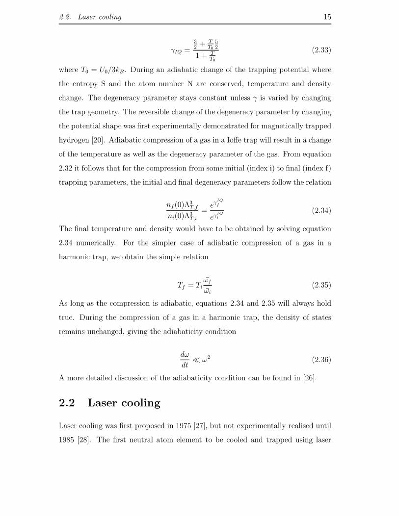
Figure 2.2: An illustration of the principles of Doppler cooling.
radiation was sodium, but the other alkali metal atoms soon followed. In 1997,
Steven Chu, Claude Cohen-Tannoudji, and William D. Phillips were awarded The
Nobel Prize in Physics ‘for the development of methods to cool and trap atoms
with laser light’. Laser cooling was a major discovery in the 20th century and was
the last piece in the jigsaw of the quest to create a Bose-Einstein Condensate.
2.2.1 Doppler cooling
Photons have energy E = hω and momentum vector ~p = h~k. The absorption of
a photon puts the atom into an excited state with a recoil from the light source
with momentum −h~k. The absorption is directional but the spontaneous emission
is purely isotropic and therefore contributes no net momentum on the atom. The
scattering force involves absorption and afterwards spontaneous emission and this
scattering force F is dependent upon the scattering rate and the recoil momentum:
F=Rh~k where scattering rate R is given as
R =Γ
2
IIs
1 + IIs
+ (2(δ−~k·~v)Γ
)2(2.37)
where Γ is the natural width of the transition, δ is the laser detuning from the
resonance (ω0 − ωL), and −~k · ~v is the Doppler shift as seen by the moving atoms.
IIs
= 2Ω2
Γ2 is the ratio between laser intensity and the saturation intensity where Ω
is the Rabi frequency.
2.2. Laser cooling 17
Consider atoms illuminated by two counter-propagating light beams of identical
intensity, polarisation and frequency. If the laser detuning is negative with respect
to the atomic resonance (‘red-detuned’), the frequency of the light of the beam
opposing the atom’s motion is Doppler shifted towards the blue in the atomic rest
frame and is therefore closer to resonance. Thus the atom absorbs photons pref-
erentially from the beam that opposes its motion. Hence the atoms experience a
viscous force opposing their motion and this force is proportional to their veloc-
ity. The same principle can be extended to three dimensions using three pairs of
counter-propagating light beams in orthogonal directions (optical molasses).
As the atoms are cooled their Doppler frequency changes. Once the velocity change
is large enough the laser radiation is no longer in resonance with the atoms and
cooling stops. There are two possible methods of compensating for the changing
Doppler shift as the atoms decelerate: changing the laser frequency [29] [30] [31],
or spatially varying the atomic resonance frequency using a magnetic field [32] [33].
The heating associated with spontaneous emission leads to a limit on the tem-
perature that can be reached using Doppler cooling. Even though the average
momentum from spontaneous emission is zero, the root-mean-square (rms) value
of the momentum is non-zero. This leads to a Brownian motion-like behaviour by
the atoms. The Doppler limit [34] is given by TD = hΓ2kB
and for Rubidium this is
146 µK.
2.2.2 Sub-Doppler cooling
Doppler cooling theory assumes a basic two-level system. However, alkali atoms
have hyperfine structure and Zeeman sublevels, so they can be cooled to tem-
peratures much lower than the Doppler limit via more sophisticated processes.
Sub-Doppler cooling depends on multiple (normally degenerate) ground states,
‘light shifts’ of ground states, optical pumping among ground states and polariza-
tion gradients in the light field. The viscous damping experienced by the atoms in
sub-Doppler cooling is much greater than that in Doppler cooling. However, the
2.2. Laser cooling 18
m =+1/2F
m =-1/2F
Excited
level
Polarization of
standing wave
s- s-s+ s+
Lin ^Lin Lin
Direction of
atom’s motion
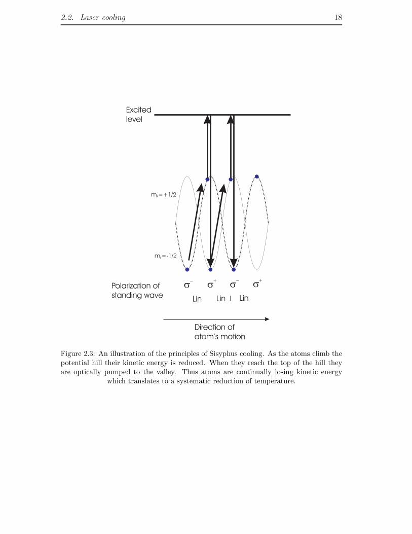
Figure 2.3: An illustration of the principles of Sisyphus cooling. As the atoms climb thepotential hill their kinetic energy is reduced. When they reach the top of the hill theyare optically pumped to the valley. Thus atoms are continually losing kinetic energy
which translates to a systematic reduction of temperature.

2.2. Laser cooling 19
cooling capture range is small so atoms must be initially Doppler cooled before
sub-Doppler cooling can occur.
When a laser beam is incident on an atom, the energy levels are perturbed by the
light field. Light shifts cause a splitting of the ground state energy. For J = 1/2,
the ground state is split into two levels mJ = +1/2 and mJ = −1/2. However,
because of the standing wave formed by two counter-propagating beams the energy
levels will vary periodically across the wavelength of the standing wave (see Figure
2.3). Another notable difference is that when the orientation of the atom (its mF
state) is taken into account, atomic interaction with the light field depends upon
the polarisation of the radiation. Different states in multilevel atoms are coupled
differently to the light field depending on the polarization, e.g. σ+ polarization
drives ∆mF = +1 transitions and σ− polarization drives ∆mF = −1 transitions.
The two important polarization cases in sub-Doppler cooling are the linear ⊥ linear
configuration and the σ+−σ− configuration. They both lead to temperatures below
the Doppler limit but by different mechanisms. A full treatment of sub-Doppler
cooling is given in [35].
For linear ⊥ linear polarisation gradient cooling, the two linearly polarized counter-
propagating beams of the same frequency interfere and create a strong polarization
gradient. The polarization changes from linear to σ+ in λ/4 (see Figure 2.3). When
the atom absorbs a photon and is excited there are two possible outcomes: the
atom decays to the original level, or it decays to a different magnetic sublevel.
For the former case the atom receives a random momentum kick and its energy
does not change. For the latter case, the spontaneously emitted photon is of
a higher frequency than the one that was absorbed (Figure 2.3). This means
that overall, the atom loses energy, leading to a reduction in its velocity and
therefore temperature. Careful selection of the laser radiation detuning makes it
more probable for an atom to absorb a photon at the top of the potential ‘hill’ than
at the bottom. This leads to a reduction in the energy of the atoms i.e. cooling.
Figure 2.3 illustrates the principles of linear ⊥ linear polarization gradient cooling.
2.2. Laser cooling 20
Linear ⊥ linear polarization gradient cooling is also called Sisyphus cooling after
the Greek mythological character Sisyphus. He was doomed by the Greek gods to
forever roll a large boulder to the top of a hill.
For σ+ − σ− polarization gradient cooling, two counter-propagating light beams
with opposite circular polarisation create a light field where the polarization re-
mains linear but rotates in direction about the beam’s axis. When the atoms travel
along the axis of the beams the light shifts of the ground state sublevels remain
constant and therefore Sisyphus cooling does not occur in this case. For a station-
ary atom the population distribution is symmetric across the magnetic sublevels
and therefore the atom absorbs photons from both beams equally resulting in no
net force on the atom. When the atoms are moving through a polarization gradi-
ent, there is a difference in the scattering rate between the two counter-propagating
beams. Since the transition rate between different pairs of magnetic sublevels of
excited and ground states (Clebsch-Gordon coefficients) depends on the orientation
of the electron spin and the polarization of the radiation driving the transition, the
atom will preferentially absorb photons from the laser beam which opposes its mo-
tion. The distribution across the magnetic substates is then no longer symmetric
and creates an imbalance in the absorption rate of photons from the two beams,
giving a net force that opposes the atom’s motion.
While the sub-Doppler viscous damping is much larger than that of the Doppler
cooling mechanism, the resultant temperature is still limited by the heating caused
by spontaneous emission. Temperatures of about one order of magnitude above the
recoil limit can be attained. The recoil temperature is given by Tr = (hk)2/mkB
and for rubidium this is Tr = 361.96 nK. While nowadays evaporative cooling is the
most widely-used technique to achieve cloud temperatures in the nK regime, there
are other laser cooling techniques used to achieve those temperatures. Two of them
are Velocity-Selective Coherent Population Trapping (VSCPT) [36] and Raman
cooling [37]. Neither Doppler nor sub-Doppler cooling contain a dependence on
position so optical molasses does not localise the atoms. In order to trap atoms,

2.3. Magneto-optical traps 21
Energy
Position
Magnetic
Field
F=0
Ground
State
F=1
Excited
State
mF= -1
mF= 0
mF= +1
-1
0
+1
-
z
wL
s+ s-
z’
d+
d-
Figure 2.4: Arrangement for a MOT in one-dimension. At point z = z′ the atoms arecloser to resonance with the σ− beam. Therefore the atom is driven towards the centreof the trap. Even though the scheme is described for F = 0 −→ F′ = 1 transition,it
works well for any F −→ F′ = F + 1 transition.
magneto-optical traps were developed.
2.3 Magneto-optical traps
Most of the cooling in a typical BEC experiment occurs in the magneto-optical
trapping (MOT) stage. Such traps use light and magnetic fields to confine large
numbers of atoms and cool them to temperatures much less than 30 µK. The first
demonstration of a MOT was in 1987 [38] and since then there has been extensive
treatment of MOTs in the literature [39], [40], [41], [42]. The various possible
MOT orientations include the four-beam MOT [43], the pyramidal MOT [44] and
the surface MOT [45].
A magnetic field needs to be present to localize the atoms in space and is normally
generated by a pair of anti-Helmholtz coils. The ground state and the excited
magnetic states are shifted in energy by the Zeeman effect. The excited state
has three Zeeman components (for a F = 1 state) and the transition frequencies

2.3. Magneto-optical traps 22
I
s-
s-
s-
I
s+
s+
s+
Figure 2.5: Direction and polarization configuration of a six beam MOT.
of these states vary with magnetic field and therefore position. The atoms are
illuminated by two red-detuned (δ < 0) counter-propagating beams of opposite
circular polarization. The imbalance in the forces experienced by the atoms by the
two beams leads to a resultant force on the atoms. A schematic of the principles
of a MOT is given in Figure 2.4.
2.3.1 Six-beam MOT
Figure 2.4 illustrated the principles of a MOT in one dimension. To extend the
principle to three dimensions two further pairs of counter-propagating beams of
opposite circular polarization are added in orthogonal directions to the original
beams. This is illustrated in Figure 2.5.
The polarization configuration in a MOT seems to imply that only σ+ − σ− po-
larization gradient cooling occurs. This would be true if the atoms moved only
along the axis of the beams. However, in practice atoms move in random directions
and therefore at intermediate points between the axes the polarization is not well
defined. At these points, both types of sub-Doppler cooling occur.

2.4. Magnetic trapping of neutral atoms 23
B B
s-
s-
s+
s+
Figure 2.6: Cross-section of the pyramidal MOT and the resulting polarization configu-ration.
2.3.2 Pyramidal MOT
The pyramidal MOT is a way of generating the same radiation field as in a six-
beam MOT, except a pyramidal MOT only requires one input beam to produce
the same configuration of light polarizations as a standard six-beam MOT. The
original pyramidal MOT consisted of a large beam of σ− polarized light incident
on a conical hollow mirror [44]. This was then modified to include a small aperture
at the vertex in order to not only confine atoms but enable transfer of atoms into
the experimental MOT [46]. The first reflection on the mirror produces a pair
of counter-propagating beams with opposite polarization. The second reflection
produces a σ+ retro-reflected beam. This occurs in all three dimensions creating the
required polarization configuration. Figure 2.6 illustrates the setup of a pyramidal
MOT.
2.4 Magnetic trapping of neutral atoms
In most BEC experiments magnetic traps are used to confine laser cooled atoms
and compress the atomic cloud in order to achieve the high collision rates needed
for efficient evaporative cooling. We shall firstly describe the atomic properties

2.4. Magnetic trapping of neutral atoms 24
that enable magnetic trapping of neutral atoms and how they are exploited for
that purpose. Then we shall describe a general class of magnetostatic traps that
confine these atoms. Magnetic trapping of neutral atoms was first observed in
1985 [47]. Shortly afterwards, orders of magnitude improvements in density and
number of trapped atoms were achieved at MIT and in Amsterdam using super-
conducting traps and different loading schemes [48] [49] [50]. Magnetic forces are
strong for atoms with unpaired electrons, such as the alkali metals, resulting in
atomic magnetic moments µ of the order of a Bohr magneton. The interaction
energy between a magnetic dipole and an external magnetic field ~B is given by
−~µ · ~B = µBcosθ. In a classical picture, the angle θ between the magnetic moment
and the magnetic field is constant due to the rapid precession of ~µ around the
magnetic field axis. For weak magnetic fields, the energy levels of the atom in
a magnetic field is E(mF ) ≈ mF gFµBB where gF is the g-factor and mF is the
quantum number related to the z-component of the total angular momentum F.
The term cos θ is replaced by mF/F since in the classical picture, a constant angle
θ is equivalent to the system remaining in the same mF state. Magnetic trapping
of atoms requires a local minimum in the magnetic potential energy E(mF ) < 0.
High-field seeking states cannot be trapped because Maxwell’s equations do not
allow a magnetic field maximum in free space [51], therefore this automatically
requires we must have our atoms in the ‘weak-field seeking states’ (mF gF > 0) for
them to be able to be trapped magnetically.
Weak-field seeking states are not the states of lowest energy thus since those mag-
netic traps only confine weak-field seeking states, atoms can be lost from the trap
by transitions to strong-field seeking states. Such transitions can be induced by
the motion in the trap because an atom sees a field in its moving frame which
is changing in magnitude and direction. The trap is only stable if the atom’s
magnetic moment adiabatically follows the direction of the magnetic field. This
requires that the rate of change of the field direction be slower than the precession
of the magnetic moment:
2.4. Magnetic trapping of neutral atoms 25
dθ
dt<µ|B|h
(2.38)
where θ is the orientation angle defined above. The upper bound for this rate of
change would be the trapping frequency. This adiabatic condition is violated in
regions of very small magnetic fields leading to trap loss by spin flips to untrapped
states. These flips are called Majorana flops [52].
2.4.1 Zeeman effect on the hyperfine ground states
Under the influence of a static magnetic field B, the Zeeman energy of the two
hyperfine levels of the ground configuration is given by the Breit-Rabi formula [53]
[54]. For the case of vanishing orbital angular momentum, this Zeeman energy is
given as
EF,mF(B) = (−1)F 1
2hωhf
√
1 +4mF
2I + 1x+ x2 + const. (2.39)
where x is given as
x =(gI + gS)µBB
hωhf
(2.40)
The numerator is the Zeeman energy and it is divided by the hyperfine splitting
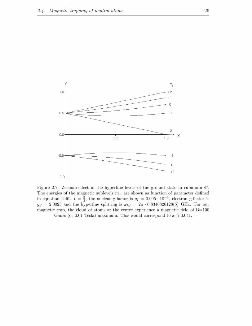
Ehf = hωhf of the ground state. Figure 2.7 shows the Zeeman effect on the
hyperfine ground state. In this graph, y is given as EF,mF(B)/hωhf in equation 2.39
chosen so that for x=0 the energies are E/hωhf = ±1/2 and x is given as equation
2.40. The small contribution from the nuclear moment is usually neglected as
gI ≪ gS.
In most static magnetic traps the magnetic fields give lower Zeeman energy than
the hyperfine splitting of the ground state. Under conditions where x ≪ 1, equa-
tion 2.39 can be approximated as
EF,mF(B)
hωhf= (−1)F [
1
2+
(−1)F
2I + 2x+
4 −m2F
16x2] (2.41)
where
2.4. Magnetic trapping of neutral atoms 26
m[
0.0
0.5
-0.5
0.5 1.0
1.0
-1.0
+2
-2
+1
-1
0
-1
0
+1
Y
X
Figure 2.7: Zeeman-effect in the hyperfine levels of the ground state in rubidium-87.The energies of the magnetic sublevels mF are shown as function of parameter definedin equation 2.40. I = 3
2 , the nucleus g-factor is gI = 0.995 · 10−3, electron g-factor isgS = 2.0023 and the hyperfine splitting is ωhf = 2π · 6.8346826128(5) GHz. For ourmagnetic trap, the cloud of atoms at the centre experience a magnetic field of B=100
Gauss (or 0.01 Tesla) maximum. This would correspond to x ≈ 0.041.
2.4. Magnetic trapping of neutral atoms 27
I I
(a) (b)
z axis ca
x axis
y axis
s
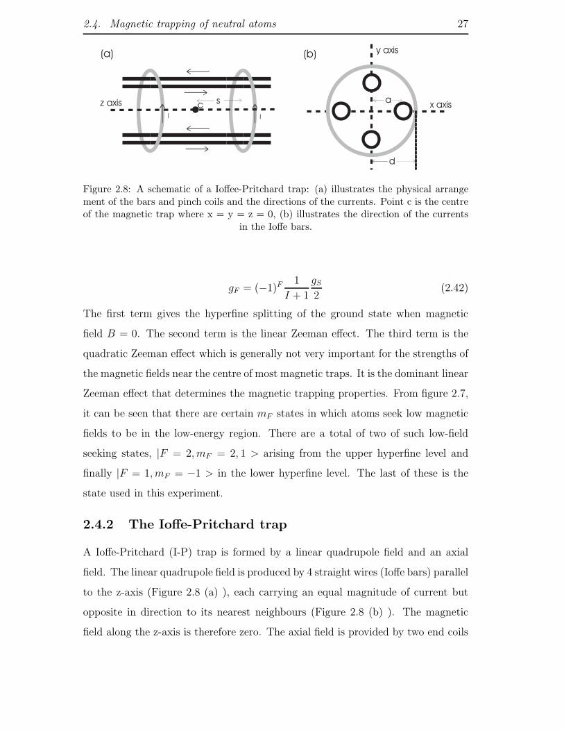
d
Figure 2.8: A schematic of a Ioffee-Pritchard trap: (a) illustrates the physical arrangement of the bars and pinch coils and the directions of the currents. Point c is the centreof the magnetic trap where x = y = z = 0, (b) illustrates the direction of the currents
in the Ioffe bars.
gF = (−1)F 1
I + 1
gS
2(2.42)
The first term gives the hyperfine splitting of the ground state when magnetic
field B = 0. The second term is the linear Zeeman effect. The third term is the
quadratic Zeeman effect which is generally not very important for the strengths of
the magnetic fields near the centre of most magnetic traps. It is the dominant linear
Zeeman effect that determines the magnetic trapping properties. From figure 2.7,
it can be seen that there are certain mF states in which atoms seek low magnetic
fields to be in the low-energy region. There are a total of two of such low-field
seeking states, |F = 2, mF = 2, 1 > arising from the upper hyperfine level and
finally |F = 1, mF = −1 > in the lower hyperfine level. The last of these is the
state used in this experiment.
2.4.2 The Ioffe-Pritchard trap
A Ioffe-Pritchard (I-P) trap is formed by a linear quadrupole field and an axial
field. The linear quadrupole field is produced by 4 straight wires (Ioffe bars) parallel
to the z-axis (Figure 2.8 (a) ), each carrying an equal magnitude of current but
opposite in direction to its nearest neighbours (Figure 2.8 (b) ). The magnetic
field along the z-axis is therefore zero. The axial field is provided by two end coils
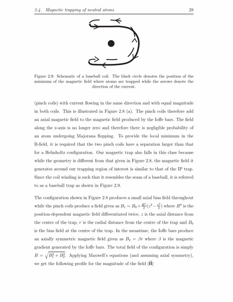
2.4. Magnetic trapping of neutral atoms 28
Figure 2.9: Schematic of a baseball coil. The black circle denotes the position of theminimum of the magnetic field where atoms are trapped while the arrows denote the
direction of the current.
(pinch coils) with current flowing in the same direction and with equal magnitude
in both coils. This is illustrated in Figure 2.8 (a). The pinch coils therefore add
an axial magnetic field to the magnetic field produced by the Ioffe bars. The field
along the z-axis is no longer zero and therefore there is negligible probability of
an atom undergoing Majorana flopping. To provide the local minimum in the
B-field, it is required that the two pinch coils have a separation larger than that
for a Helmholtz configuration. Our magnetic trap also falls in this class because
while the geometry is different from that given in Figure 2.8, the magnetic field it
generates around our trapping region of interest is similar to that of the IP trap.
Since the coil winding is such that it resembles the seam of a baseball, it is referred
to as a baseball trap as shown in Figure 2.9.
The configuration shown in Figure 2.8 produces a small axial bias field throughout
while the pinch coils produce a field given as B1 = B0+ B′′
2(z2− r2
2) where B′′ is the
position-dependent magnetic field differentiated twice, z is the axial distance from
the centre of the trap, r is the radial distance from the centre of the trap and B0
is the bias field at the centre of the trap. In the meantime, the Ioffe bars produce
an axially symmetric magnetic field given as B2 = βr where β is the magnetic
gradient generated by the Ioffe bars. The total field of the configuration is simply
B =√
B21 +B2
2 . Applying Maxwell’s equations (and assuming axial symmetry),
we get the following profile for the magnitude of the field |~B|
2.5. Evaporative cooling 29
|~B| ≈ B′′z2 +( β2
B0
− B′′
2
)
r2 (2.43)
for very small clouds where the trapping potential can be well-approximated by
an anisotropic harmonic potential.
The Ioffe-Pritchard trap has two different regimes. For temperature kBT < µB0,
the cloud experiences the potential of a 3D anisotropic harmonic oscillator. For
kBT > µB0, the potential is linear along the radial direction and harmonic along
the axial direction.
From equation 2.43, it can be seen immediately that we can tighten the radial
trapping frequency by lowering B0 whilst keeping β constant. Experimentally, this
is usually carried out using a pair of compensation coils (bias coils) whose field is
set to null the magnetic field at the centre of the original Ioffe trap. The overall
field at the centre of the trap must remain high enough to suppress Majorana flops,
i.e. about 1 G. To fine-tune the remaining field after cancellation, we have another
pair of coils called the secondary bias coils. Low-fields can be achieved with the
combination of the bias coils and the baseball trap. Implementation of current
control will be described in the next chapter.
2.5 Evaporative cooling
Unlike standard laser cooling, evaporative cooling can go below the recoil limit.
This method is analogous to evaporation of a cup of coffee. The energetic particles
escape the cup and then the remaining particles rethermalise to a new thermal
equilibrium at a temperature lower than that initially because the average energy of
the system has fallen. For atoms in magnetic traps, the hotter atoms are removed
by inducing RF transitions. This cooling method clears the final hurdle before
Bose-Einstein Condensation and to date, some form of evaporative cooling has
been used in all experiments where condensates are formed. This technique is a
very useful cooling method that does not suffer from the limitations which exist
2.5. Evaporative cooling 30
with optical cooling method like the Doppler-limit and the recoil limit. The idea
of evaporative cooling was first introduced for trapped atomic hydrogen [49]. A
review on evaporative cooling is given by [55] and [56].
2.5.1 Evaporative cooling
Here we briefly sketch the principles of evaporative cooling. The description is
based on the model of evaporative cooling as introduced by [19] and [56]. Evap-
orative cooling is based on the preferential removal of atoms with energy above
a certain truncation energy ǫt from the trap and subsequent thermalization by
elastic collisions. For a constant truncation barrier ǫt (plain evaporation) elastic
collisions between atoms in a trap produce atoms of energies higher than ǫt which
are removed (or ’evaporated’) from the trap. The evaporation rate per atom is
given as
τ−1ev =
Nev
N= n(0)υTσe
−ηVev
Ve
(2.44)
where σ=8πa2=7.9 × 10⁻¹⁶ m2 is the elastic collision cross section, and the trun-
cation parameter η is given by
η =ǫtkBT
(2.45)
assuming that Vev = Ve is the effective volume for evaporation [56]. As hotter atoms
are ejected from the trap, the average energy of the cloud falls. As the temperature
has been reduced, η becomes larger and the evaporation rate is exponentially
suppressed. For a continuous cooling process, the truncation energy ǫt is reduced
such that η remains constant (forced evaporative cooling). For forced evaporative
cooling at constant η,
T ∝ Nαev (2.46)
where the efficiency parameter
2.5. Evaporative cooling 31
αev =dln(T )
dln(N)(2.47)
depends only on the truncation parameter η. During evaporative cooling, the
effective volume also decreases and this can be expressed as
Ve ≈ T δ (2.48)
where δ = 5/3 for a Ioffe trap at high temperatures (the linear limit) and δ = 3/2
for a Ioffe trap at low temperatures (harmonic limit). Combining equations 2.46
and 2.48 and the definition Ve ≈ N/n(0) shows that despite significant loss of
atoms during the evaporation process, the peak cloud density at the centre of the
trap can remain constant or even increase provided that αev ≥ 1/δ. Given that
the elastic collision rate is τ−1el ∝ n(0)T
1
2 , even though temperature decreases, the
increase in density can be large enough that the ‘runaway’ evaporative cooling
condition remains fulfilled, namely
dln(n√T )
dln(N)= 1 − 2αev < 0 (2.49)
In practice, evaporative cooling is limited by various loss processes like background
collisions where atoms collide with particles in the vacuum background and for very
high densities, two-body and three-body inelastic collisions. In general, the atomic
loss rate τ−1i for i-body collisions is expressed by the rate constant Gi given as
τ−1i ≡ Ni
N= −Gin(0)(i−1)Vie
Ve
(2.50)
where the reference volumes for i-body collisions are defined as
Vie ≡∫
dr
(
n(r)
n(0)
)i
(2.51)
For two and three-body inelastic collisions, these reference volumes can be calcu-
lated numerically while for background collisions this reference volume is simply
the one introduced in equation 2.16. Evaporative cooling is most efficient for large
ratio Ri which is the ratio between the elastic collision rate and the rate of the

2.5. Evaporative cooling 32
various loss processes. This ratio is also sometimes called ‘ratio of good to bad
collisions’ given by
Ri ≡Nev
Ni
=n(0)υTσ
Vev
Vee−η
n−1(0)GiVie
Ve
≡ 1
λi
Vev
Ve
e−η (2.52)
In this case,
λ1 =τ−1i
τ−1el
=n(i−2)(0)Gi
υTσ
Vie
Ve
(2.53)
and where the elastic collision rate is given as
τ−1el = n(0)συT (2.54)
In typical BEC experiments, in the earlier stages of evaporative cooling the peak
density for most initial clouds is low enough that only background collisions need
to be considered.
2.5.2 RF-evaporative cooling
As mentioned above, evaporative cooling is performed by selectively removing the
hotter atoms from the trap so that the gas cloud then cools down. The energy
selective removal of the atoms from the trap is achieved by driving atomic transi-
tions from trapped states to untrapped Zeeman states with an oscillating magnetic
field of angular frequency ωrf . The atoms undergo the transitions only at positions
where the resonance condition
hωrf = gFµB|B(r)| (2.55)
is achieved. So the truncation energy ǫt at which atoms in the state mF are ejected
from the trap is related by the interaction energy of an atom with an external
magnetic field E = −µ · B and the radio frequency ωrf by
ǫt = mF h(ωrf − ω0) (2.56)
2.6. Sub-shot noise measurements of atom number 33
where ω0 = gFµB|B(0)|/h is the resonance radio frequency at the centre of the trap.
Experimentally, evaporative cooling is performed by lowering the radio frequency
from a starting value towards the resonance frequency in specific stages where each
stage is optimised by measuring the resulting phase space density.
2.6 Sub-shot noise measurements of atom num-
ber
In this section, we give a theoretical introduction to the project that we want
to implement after obtaining BEC, in particular dipole trapping and aspects of
this technique relevant to the experiments we wish to do. The next part then
talks about the Mott Insulator State which we want to achieve as a preliminary to
quantum information processing.
2.6.1 Dipole trapping of neutral atoms
This subsection is divided into two parts. Firstly, we obtain the two important
properties of dipole traps, the dipole potential and the scattering rate. Then we
discuss red-detuned dipole trapping which is more relevant to us. A more formal
treatment of dipole trapping can be found in [57].
The dipole potential
When an atom is illuminated by laser light, the electric field ~E induces an atomic
dipole moment ~p which oscillates with a frequency equal to its driving frequency
ω. The amplitude p is related to the electric field amplitude E by the relation
p = αE where α is the complex polarisability of the atom dependent upon ω.
The electric field and the induced dipole moment are given in their usual complex
notations ~E(r, t) = eE(r) exp(−iωt)+c.c and ~p(r, t) = ep(r) exp(−iωt)+c.c where
e is the unit polarisation vector. Given these, the interaction potential between
the electric field and the induced dipole moment is given as
2.6. Sub-shot noise measurements of atom number 34
Udip = −1
2< ~p~E >= − 1
2ǫ0cRe(α)I (2.57)
where I is the field intensity I = 2ǫ0c|E|2, ǫ0 is the electric constant and c is the
speed of light in vacuo. The power absorbed by the atom in the oscillator model
and re-emitted as dipole radiation is given by
Pabs =< p ~E >=ω
ǫ0cIm(α)I (2.58)
Now if we consider the light as a stream of photons each with energy hω, this ab-
sorption can be interpreted as scattering with cycles of absorption and reemission.
The scattering rate is then given by
Γsc(r) =Pabs
hω=
1
hǫ0cIm(α)I(r) (2.59)
Note that now we have expressed field intensity as a position-dependent variable
which is a more realistic view of beam intensities. These expressions are valid for
any polarisable neutral particle in some oscillating electric field.
To calculate the polarisability term α, we first consider the atom in Lorentz’s
model of a classical oscillator and view the electron of mass me and charge e as
bound elastically to the core with an oscillation frequency ω0 corresponding to the
optical transition frequency. We then calculate the polarisability by integration of
the electron’s equation of motion x+ Γωx+ ω20x = −eE(t)
mwith the result
α =e2
me
1
ω20 − ω2 − iωΓω
(2.60)
where
Γω =e2ω2
6πǫ0mec3(2.61)
Introducing the on-resonance damping rate Γ = (ω0/ω)2Γω, equation 2.60 becomes
α = 6πǫ0mec3 Γ/ω2
0
ω20 − ω2 − iω3/ω2
0Γ(2.62)
2.6. Sub-shot noise measurements of atom number 35
In the semiclassical approach, the atom must be treated as a two-level quantum
system interacting with a radiation field. The damping rate (or scattering rate
now) is determined by the dipole matrix element between the ground state and
the excited state. However, for the D lines of alkali atoms such as Na, K, Rb
and Cs, the classical result agrees with the true spontaneous decay rate of the
excited state to within a few percent. In fact, for many atoms with a strong
dipole-allowed transition from the ground state, the classical formula provides a
very good approximation to its true decay rate.
So given the expression for polarisability and also for low saturation and large
detunings, the dipole potential and scattering rate are given as
Udip(r) = −3πc2
2ω30
(Γ
ω0 − ω+
Γ
ω0 + ω)I(r) (2.63)
Γsc(r) =3πc2
2hω30
(ω
ω0)3(
Γ
ω0 − ω+
Γ
ω0 + ω)2I(r) (2.64)
In most experiments, the laser frequency is sufficiently close to the transition fre-
quency such that the detuning ∆ = ω−ω0 fulfills the inequality |∆| ≪ ω0. In this
case, we can apply the rotating-wave approximation [58] and set ω/ω0 ≈ 1. The
general case for optical potentials and scattering rate then simplifies to
Udip(r) =3πc2
2ω30
Γ
∆I(r) (2.65)
Γsc(r) =3πc2
2hω30
(
Γ
∆
)2
I(r) (2.66)
These expressions tell us two important features of dipole trapping. The first is
the interaction with respect to the sign of the detuning. For red-detuned dipole
traps which we will be working with, ∆ < 0 and this tells us that the atoms
tend to move towards regions of high field intensity where there is a potential
minima. However, for blue detuning ∆ > 0, atoms stay away from regions of high
intensity. The second is the scaling with intensity and detuning. While the dipole
potential is inversely proportional to ∆, scattering rate is inversely proportional
2.6. Sub-shot noise measurements of atom number 36
to ∆2. Therefore, for a certain potential depth, it would be useful to have dipole
traps with large detunings and high intensities.
The focused beam trap
There are three types of red-detuned dipole traps. They are the focused beam
trap, the standing wave trap and the crossed-beam trap. We shall concentrate on
the focused beam trap because this trap type is the one we shall be using in our
experiment.
The focused beam trap is the simplest type of dipole trap that provides three-
dimensional confinement of atoms and is formed by nothing more than one beam
which focuses via some lens onto a spot of high light intensity. The spatial intensity
distribution of a focused Gaussian beam (FB) with power P propagating along the
z-axis is given by
IFB(r, z) =2P
πw2(z)exp(−2
r2
w2(z)) (2.67)
where r is the radial coordinate. The 1/e2 radius of the beam w(z) depends on
the axial coordinate z via
w(z) = w0
√
1 +(
z
zR
)2
(2.68)
where Rayleigh length is zR = πw20/λ. The trap depth is given by U = Udip(r =
z = 0). If the thermal energy kBT is much smaller than the trap depth U , then
the dipole potential can be approximated by an harmonic oscillator:
U(r) ≈ −U [1 − 2(r
w0)2 − (
z
zR)2] (2.69)
and the oscillation frequencies are given by ωr =√
4U/mw20 and ωz =
√
2U/mz2R.
Automatically, the radial frequency frequency is always tighter than the axial fre-
quency by a factor of ωr/ωz =√
2π2
λ2 ω20.
2.6. Sub-shot noise measurements of atom number 37
2.6.2 The Mott Insulator State
With the theory of dipole trapping established, experimental realisation of such
traps was the next step towards quantum computation with neutral atoms. We
begin with the 1D optical lattice where one pair of counter-propagating laser beams
interfere and gives a trap potential in 1D while the atoms are weakly trapped
by a magnetic field in the other two dimensions. Loading of BEC into a 1D
dipole trap was first achieved by Stamper-Kurn et al [59] and this 1D version
could theoretically be extended to the 3D version with three pairs of counter-
propagating laser beams instead of one. There are many novel features of a BEC
loaded into a 3D lattice and one of them is the demonstration of the transition
between the superfluid state and the Mott Insulator state [8]. We wish to reproduce
the Mott insulator state of our atom cloud before moving on to qubit operations
with neutral atoms. This section gives an introduction to the dynamics of a BEC in
an optical lattice (or arrays of dipole traps in general) brought about by interatomic
interactions.
We start by writing the Hamiltonian operator for bosonic atoms in some external
trapping potential
H =∫
d3xψ†(r)
(
− h2
2m2 +V (r) + VT (r)
)
ψ(r)+1
2
4πash2
m
∫
d3xψ†(r)ψ†(r)ψ(r)ψ(r)
(2.70)
with ψ(r) being a boson field operator for atoms in some given state, V (r) being
the potential related to an optical lattice or an array of dipole traps and VT (r) be-
ing an additional slow-varying external trapping potential like a magnetic trapping
potential. The interaction between the atoms is approximated by a short-range
pseudopotential with as being the s-wave scattering length and m being the mass
of the atoms. For single atoms the eigenstates are Bloch wavefunctions and the
superposition of these wavefunctions provide a set of Wannier functions well lo-
calised on individual lattice sites. We assume the energy of the atoms is much
less than the excitation energy to the second Bloch band. If we were to expand
2.6. Sub-shot noise measurements of atom number 38
the field operators in the Wannier basis and keep only the lowest vibrational levels
ψ(r) = Σibiw(r − ri), equation 2.70 reduces to the Bose-Hubbard Hamiltonian
(BHM)
H = −JΣi,jb†ibj + Σiǫini +
1
2UΣini(ni − 1) (2.71)
where ni = b†ibi count the number of atoms at lattice site i and where the annihila-
tion and creation operators bi and b†i obey the commutation relations [bi, b†j ] = δij .
U = 4πash2 ∫ d3x|w(r)|4/m corresponds to the interaction strength of on site re-
pulsion between two atoms on site i, J =∫
d3xw∗(r−ri)[− h2
2m2+V (r)]w(r−rj) is
the hopping matrix element between adjacent sites i, j and ǫi =∫
d3xVT (r)|w(r−ri)|2 ≈ VT (ri) describes the energy offset of each site provided by the slowly varying
external potential.
The BHM predicts that there will be a phase transition between the superfluid
(SF) state and the Mott insulator (MI) state at low temperatures and when the on
site interaction energy U is much larger than the tunneling matrix element J [60].
In an optical lattice the interaction energy U can be increased by increasing the
laser intensity to make the atomic wave function more and more localised while
the tunneling matrix element is reduced. According to mean-field theory [60], the
critical value of the MI-SF transition for the n = 1 phase is at U/zJ ≈ 5.8 with
z = 2d being the number of nearest neighbours. The dipole trap depth required
for this transition is typically in the few tens of recoil energies. At MI stage the
occupation number per site is pinned at integer n = 1, 2, ... and this corresponds to
a commensurate filling of the optical lattice. This system therefore represents an
optical crystal. Another way of looking at this phase transition is in terms of the
Heisenberg uncertainty relation involving the uncertainty in the number of atoms
in the system and the uncertainty in the phase of the macroscopic wave function
∆N · ∆φ ≥ h2. In the MI stage the uncertainty in the number of atoms reduces
to that below the Standard Quantum Limit (SQL) while phase definition suffers.
When this phase transition was first observed [8], the creation of the MI state was

2.6. Sub-shot noise measurements of atom number 39
inferred by the gradual blurring of interference patterns caused by the increase
in phase fluctuations between atoms at various lattice sites as the laser intensity
was increased. Alternatively, this state can be observed by direct atom-number
counting [61].

Chapter 3
The Experimental Apparatus
This chapter records details of the experimental apparatus largely rebuilt at the end
of the previous caesium experiment. This setup is different from other rubidium
BEC experiments in the groups and these methods are therefore not described
elsewhere.
3.1 The BEC Apparatus
3.1.1 Lasers
We have two external cavity diode lasers (Toptica DL100) operating at the D2 line
of rubidium at wavelength of λ = 780 nm. The first, referred to as the Master
laser, supplies the light we need for the cooling transitions in the pyramidal and
science MOTs and for the probe and optical pumping light. The second laser
generates the repumping light for both MOTs. The operation of a laser diode for
spectroscopic applications demands a highly stable current control and an active
control of the laser diode temperature (both at about 21.50C). We use commercial
plug-in control modules for the current (Toptica DCC 110) and for the temperature
(Toptica DTC 110). In our lasers, the external cavity is formed by a reflection
grating and the rear facet of the diode. The grating is mounted in the Littrow
configuration, i.e. the first diffraction order of the grating is reflected back towards
the diode. A diffraction-limited lens between the grating and the diode collimates
40

3.1. The BEC Apparatus 41
the light emitted from the front facet of the diode and focusses the back reflected
first order light into the diode resonator. The zeroth-order reflection serves as the
output beam providing around 50 mW of output power. In such a configuration the
feedback of the grating is highly frequency-selective, hence it provides a convenient
way to adjust the wavelength. The lasers have a line width of less than 1 MHz,
which is several orders of magnitude smaller than that of a free-running laser diode.
There is a piezo actuator integrated in the grating holder which allows changing
the cavity length and hence tuning of the laser frequency over a range of a few
GHz. We use the piezo actuator together with the current control to lock the lasers
to the required frequencies.
Aim Transition Detuning (MHz) DurationLaser Cooling F=2 −→ F’=3 -10 Until CMOT stageRepumping F=1 −→ F’=2 0 Throughout cooling processes
CMOT F=2 −→ F’=3 0 2 msMolasses F=2 −→ F’=3 -30 10 ms
Optical pumping F=2 −→ F’=2 0 0.9 msProbing F=2 −→ F’=3 0 0.2 ms
3.1.2 The optical table
The main optical table is divided into two sections: the lasers section and then the
magnetic trap section. The laser section contains all the optics required to produce
the light required for cooling, repumping, optical pumping and probing as shown in
Figure 3.1. There are two other lasers on the bench to amplify frequency-stabilised
light. They are the pyramid slave laser and the experimental MOT slave laser.
The shape of the output laser beams from both master and the repumper lasers are
firstly changed from an elliptical shape to a circular shape using anamorphic prism
pairs. These laser beams then travel through an optical isolator which prevents
optical feedback back towards the lasers which would ruin their frequency stability.
A small portion of the beam (typically much less than 1 mW) is then picked off
to a saturated absorption spectroscopy setup for frequency locking the mechanism
for which will be described in the next section. Using a half-wave plate and a
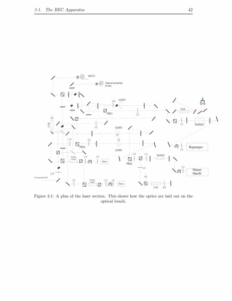
3.1. The BEC Apparatus 42
l/2
Isolator
Cell l/4
Repumper
Master90mW
Isolator
Cell
AOM1
l/2
Slave
Faradayrotator
l/2
AOM3
AOM2
l/2
To Pyramidal MOT
l/4
MOT2
Cell
Faradayrotator
l/2
Slave
l/2
Optical pumping/
Pr obe
l/4
PBS1
PBS2
PBS3
l/2
l/2
l/2
l/2
l/2
l/2
l/2
l/2l/2
Figure 3.1: A plan of the laser section. This shows how the optics are laid out on theoptical bench.
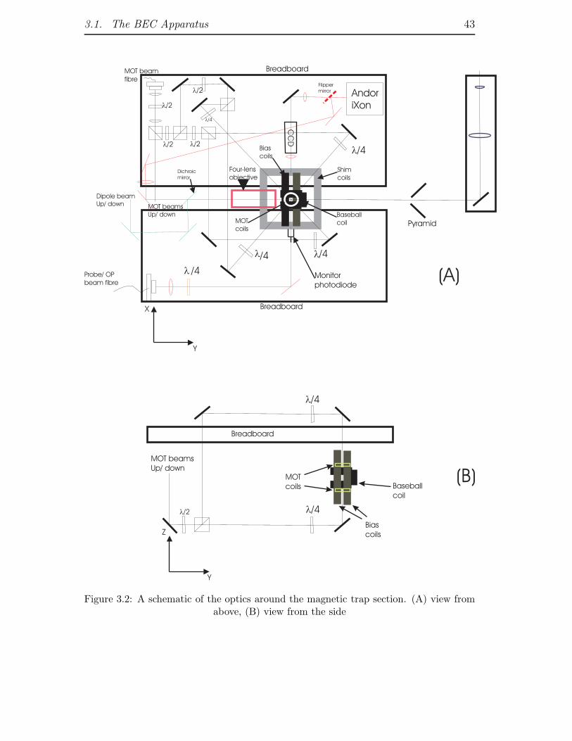
3.1. The BEC Apparatus 43
l/4
l/4 l/4
l/4
l/2
l/2 l/2
l/2
MOT beams
Up/ down
Flipper
mirror Andor
iXon
Dichroic
mirror
Dipole beam
Up/ down
l /4Probe/ OP
beam fibre
MOT beam
fibre
Four-lens
objectiveShim
coils
Bias
coils
Baseball
coilMOT
coils
CC
DMonitor
photodiode
Breadboard
Breadboard
Pyramid
MOT beams
Up/ down
l/2
l/4
l/4
Breadboard
Baseball
coil
Bias
coils
MOT
coils
Z
Y
X
Y
(A)
(B)
Figure 3.2: A schematic of the optics around the magnetic trap section. (A) view fromabove, (B) view from the side
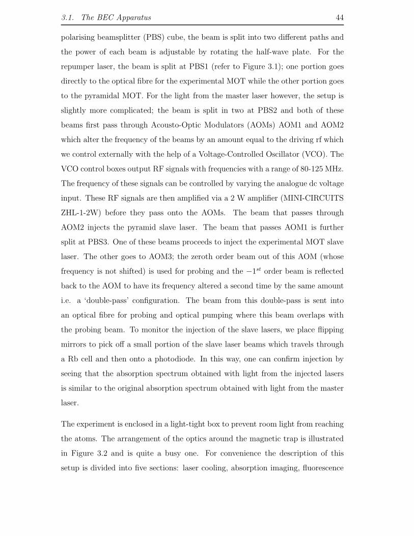
3.1. The BEC Apparatus 44
polarising beamsplitter (PBS) cube, the beam is split into two different paths and
the power of each beam is adjustable by rotating the half-wave plate. For the
repumper laser, the beam is split at PBS1 (refer to Figure 3.1); one portion goes
directly to the optical fibre for the experimental MOT while the other portion goes
to the pyramidal MOT. For the light from the master laser however, the setup is
slightly more complicated; the beam is split in two at PBS2 and both of these
beams first pass through Acousto-Optic Modulators (AOMs) AOM1 and AOM2
which alter the frequency of the beams by an amount equal to the driving rf which
we control externally with the help of a Voltage-Controlled Oscillator (VCO). The
VCO control boxes output RF signals with frequencies with a range of 80-125 MHz.
The frequency of these signals can be controlled by varying the analogue dc voltage
input. These RF signals are then amplified via a 2 W amplifier (MINI-CIRCUITS
ZHL-1-2W) before they pass onto the AOMs. The beam that passes through
AOM2 injects the pyramid slave laser. The beam that passes AOM1 is further
split at PBS3. One of these beams proceeds to inject the experimental MOT slave
laser. The other goes to AOM3; the zeroth order beam out of this AOM (whose
frequency is not shifted) is used for probing and the −1st order beam is reflected
back to the AOM to have its frequency altered a second time by the same amount
i.e. a ‘double-pass’ configuration. The beam from this double-pass is sent into
an optical fibre for probing and optical pumping where this beam overlaps with
the probing beam. To monitor the injection of the slave lasers, we place flipping
mirrors to pick off a small portion of the slave laser beams which travels through
a Rb cell and then onto a photodiode. In this way, one can confirm injection by
seeing that the absorption spectrum obtained with light from the injected lasers
is similar to the original absorption spectrum obtained with light from the master
laser.
The experiment is enclosed in a light-tight box to prevent room light from reaching
the atoms. The arrangement of the optics around the magnetic trap is illustrated
in Figure 3.2 and is quite a busy one. For convenience the description of this
setup is divided into five sections: laser cooling, absorption imaging, fluorescence
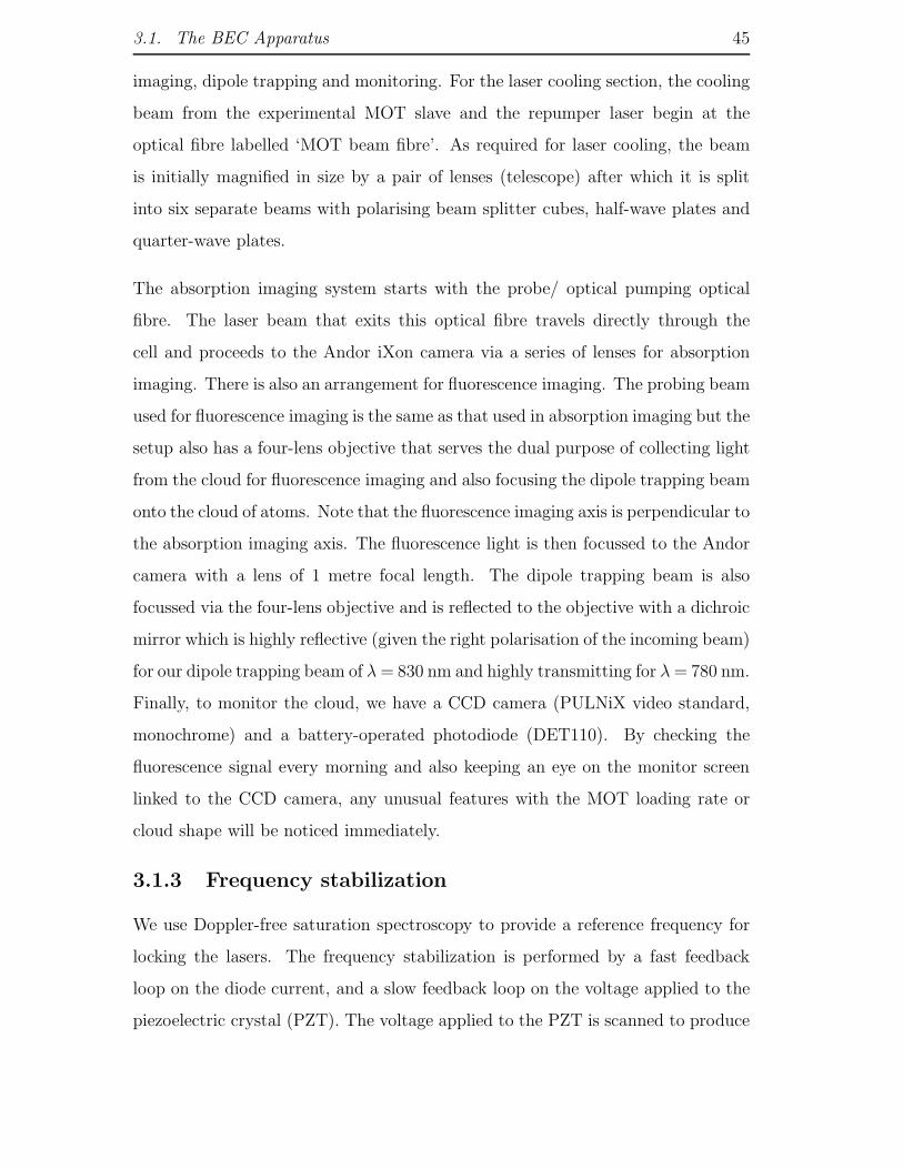
3.1. The BEC Apparatus 45
imaging, dipole trapping and monitoring. For the laser cooling section, the cooling
beam from the experimental MOT slave and the repumper laser begin at the
optical fibre labelled ‘MOT beam fibre’. As required for laser cooling, the beam
is initially magnified in size by a pair of lenses (telescope) after which it is split
into six separate beams with polarising beam splitter cubes, half-wave plates and
quarter-wave plates.
The absorption imaging system starts with the probe/ optical pumping optical
fibre. The laser beam that exits this optical fibre travels directly through the
cell and proceeds to the Andor iXon camera via a series of lenses for absorption
imaging. There is also an arrangement for fluorescence imaging. The probing beam
used for fluorescence imaging is the same as that used in absorption imaging but the
setup also has a four-lens objective that serves the dual purpose of collecting light
from the cloud for fluorescence imaging and also focusing the dipole trapping beam
onto the cloud of atoms. Note that the fluorescence imaging axis is perpendicular to
the absorption imaging axis. The fluorescence light is then focussed to the Andor
camera with a lens of 1 metre focal length. The dipole trapping beam is also
focussed via the four-lens objective and is reflected to the objective with a dichroic
mirror which is highly reflective (given the right polarisation of the incoming beam)
for our dipole trapping beam of λ= 830 nm and highly transmitting for λ= 780 nm.
Finally, to monitor the cloud, we have a CCD camera (PULNiX video standard,
monochrome) and a battery-operated photodiode (DET110). By checking the
fluorescence signal every morning and also keeping an eye on the monitor screen
linked to the CCD camera, any unusual features with the MOT loading rate or
cloud shape will be noticed immediately.
3.1.3 Frequency stabilization
We use Doppler-free saturation spectroscopy to provide a reference frequency for
locking the lasers. The frequency stabilization is performed by a fast feedback
loop on the diode current, and a slow feedback loop on the voltage applied to the
piezoelectric crystal (PZT). The voltage applied to the PZT is scanned to produce

3.1. The BEC Apparatus 46
l/2l
Isolator
Cell l/4
Master90mW
l/2
ServoResponse
Modulation/
feedback
(A)
l/2
Repumper
Isolator
Cell
Servo
Response
Modulation/
feedback
(B)
Neutral
density
filter
Substrate
Partially-
transmitting
mirror
Figure 3.3: The optical arrangements for saturated absorption spectroscopy that areused for (A) Master laser and (B) Repumper laser.

3.1. The BEC Apparatus 47
10kOhm
10kOhm
22kOhm
22kOhm
100Ohm
0.5MOhm
TL081
+V
-V
+
-
Vout
Figure 3.4: Diagram of the double photodiode (BPX65) circuit. The basic circuit is acurrent-to-voltage converter. The difference in the two photocurrents is converted into
a voltage by the operational amplifier (TL081).
an absorption spectrum where we can see the atomic transitions. Figure 3.3 shows
the layout for the absorption spectrum of both the master laser and the repumper
laser and their frequency-lock setups.
In the absorption spectrum scheme for the master laser, a filter is attached to the
quarter-wave plate to attenuate the power of the pump beam twice. This twice-
attenuated beam then acts as the probe beam in the usual saturation absorption
spectroscopy scheme.
The repumper transition is a rather weak one and therefore to obtain good signals,
we used the arrangement as shown in 3.3 (B) where an initial beam passes through
a substrate (uncoated mirror). About 90% power is transmitted and the remaining
10% is shared between two reflected beams from the front and back surface of the
substrate. One of these reflected beams acts as a probe beam counter-propagating
with the pump beam and the other as a reference beam. The beam that overlaps
the pump beam will show the saturated absorption feature while the other has

3.1. The BEC Apparatus 48
(A) Master
(B) Repumper
0
0-1
1
0-2
1-2
2
81
MHz
1-2
2
1-3
2-3
3
133
MHz
Relative frequency/ MHz
Sig
na
l stre
ng
th(a
rbitr
ary
)
Figure 3.5: Doppler-free absorption spectroscopy. (A) Master laser, transitions startfrom F=2 ground state. ”1-2” means the F’=1, F’=2 crossover. (B) Repumper laser,
transitions start from F=1 ground state.

3.1. The BEC Apparatus 49
the Doppler-broadened profile. These beams pass through a partially-transmitting
mirror to fall onto the double-photodiode in which the two photodiode signals
are subtracted to remove the Doppler background resulting in only the transition
peaks (Figure 3.5(B)). The layout of the double-photodiode circuit is shown in
Figure 3.4. In addition to subtracting the Doppler profile to make the transitions
more visible, we also heat the cell to about 370C to increase the vapour pressure
of rubidium.
We dither the current driving the diode lasers with a small amplitude to produce
a small frequency modulation at 100 kHz. When the frequency of the laser is
resonant with one of the absorption peaks, the frequency modulation produces
an amplitude modulation on the photodiode signal. The servo electronics is used
to generate an error signal from this modulation which is integrated and used as
feedback for the diode current and the amplifier for the PZT. In the absence of
external mechanical noise on the optical table, we can keep the lasers locked for
an entire day at a time. The staff of the Electronics Workshop of the Physics
Department designed and built both the lock-in electronics (EW 1225) and the
piezo driver (EW 1145).
3.1.4 Vacuum system
The vacuum system shown in Figure 3.6 has two differential pumping stages.
In the first section of the vacuum system there is pyramidal MOT. It has a pressure
of approximately 10−9 mbar maintained by a 40 l/s ion pump (Varian VacIon Plus
40). The rubidium source is several dispensers (SAES Getters) connected in series
located just above the pyramid mirrors. A current is passed through the dispensers
to heat them and the resulting chemical reaction releases the rubidium atoms. The
dispenser is continuously operated at 3.2 A to provide ample Rb pressure in the
pyramidal region.
Differential pumping is achieved by a hole (5mm diameter, 17mm long) in the
back port of the pyramid chamber. The distance between the pyramidal MOT

3.1. The BEC Apparatus 50
Ion pump
40 l/s
Ion pump
55 l/s
valve
Getter pump
Dista
nc
e b
etw
ee
n M
OTs
30
0 m
m
Pyramidal MOT
Glass cell
Figure 3.6: The vacuum system.
and the experimental MOT is 30 cm. This distance is short in order to reduce
atom loss due to divergence of the atomic beam from the pyramidal MOT to the
experimental MOT.
The ultra-high vacuum part of the vacuum system contains a rectangular quartz
cell of dimensions 28 × 28× 80mm3 (2mm wall thickness). Pressure in this region
is maintained by a 55 l/s ion pump (Varian VacIon Plus 55) and a non-evaporable
getter (NEG) pump (SAES CapaciTorr-CF35, Cartridge C-400-DSK-St172). The
NEG pump establishes ultra-high vacuum by pumping away hydrogen which is the
dominant residual gas in a clean vacuum system.
3.1.5 Pyramidal MOT
The purpose of the pyramidal MOT [62] is to collect atoms from a vapour of ru-
bidium. The atoms are transferred continuously through the differential pumping
hole into an ultra-high vacuum region, where our final experiments are performed.
Our pyramid ( Figure 3.7 ) is larger than the one described in [63]. This is an im-
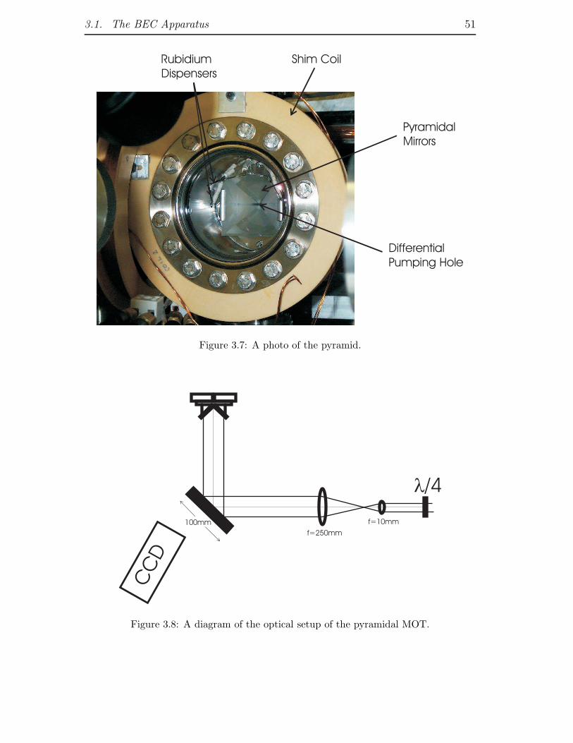
3.1. The BEC Apparatus 51
Shim Coil
Pyramidal
Mirrors
Rubidium
Dispensers
Differential
Pumping Hole
Figure 3.7: A photo of the pyramid.
f=250mm
100mm f=10mm
CC
D
l/4
Figure 3.8: A diagram of the optical setup of the pyramidal MOT.
3.1. The BEC Apparatus 52
provement as an increase in the size of the pyramidal mirrors increases the volume
of the collection region, which results in a higher flux atomic beam.
The optical setup for the pyramidal MOT apparatus is shown in Figure 3.8. The
large mirror (diameter = 100mm) and the pyramidal mirrors (base length = 60mm)
are coated by Mr C. Goodwin in the Oxford Physics Department. The mirror and
pyramid optics are coated to achieve the same reflectivity for s- and p-polarization.
(Non-equal reflectivity of s- and p-polarised light would cause a phase shift between
the two polarizations and therefore the light would no longer be circularly polarized
after reflection.)
The laser beams travelling towards the pyramidal setup consist of the cooling beam
from the pyramid slave laser and some beam coming from the repumper laser. For
the cooling beam, we begin with a measured beam waist of about 440 µm (1e
half-width). With a combination of lenses with focal lengths f=10 mm and f=250
mm, the beam is magnified and collimated after which it travels to the pyramidal
mirrors. The large beam has a waist size of 11.8 mm (1e
half-width) and contain 44
mW of cooling beam power and 6 mW of repumper beam power. We do not use
an optical fibre for this setup but this did cause some inconvenience; due to the
long path length from the laser to the pyramidal mirror, any slight changes in the
angle of the grating of the ECDL causes a deviation in the incident position of the
beam on the pyramidal mirrors. This led to a change in the loading performance
of the pyramid and meant that it was necessary to adjust the large pyramid mirror
occasionally. Fortunately, these changes are minor. It is useful to monitor the
pyramidal MOT using an infrared CCD camera.
Two sets of coils are required for generation of the magnetic fields required: a pair
of anti-Helmholtz quadrupole coils (pyramid coils), and three shim coils (pyra-
mid shim coils) positioned in orthogonal directions. The anti-Helmholtz coils pro-
vide the field gradient required for trapping of the atoms. They have 15 turns of
3mm outer diameter 22 swg (corresponding to an inner diameter of approximately
1.5mm) annealed copper tubing. Water is passed through the copper tubing to

3.1. The BEC Apparatus 53
provide cooling. The radius of the coils is 56mm and their separation is 50 mm.
To load the atoms 28A is run through the coils producing an axial field gradient
of 14 G/cm. The total resistance of the pyramid quadrupole coils (in series) and
the connecting cables is approximately 0.08Ω.
The shim coils are circular coils, inner diameter of approximately 150 mm, wound
with 100 turns of 1 mm enamelled copper wire. These shim coils serve two pur-
poses: firstly to counteract any ambient magnetic fields (e.g. earth’s magnetic
field), and secondly to move the centre of the magnetic field produced by the
quadrupole coils for diagnostic purposes. At optimal loading rate of atoms in the
second MOT, the centre of the pyramidal MOT is normally directly over the pyra-
mid hole and therefore no (or very little) fluorescence is observed. To accurately
determine the number of atoms in the pyramid it is necessary to move the centre
of the MOT to a position where the fluorescence light can be measured. The shim
coils were used only initially to measure fluorescence signal. These shim coils have
not been used since.
3.1.6 2nd MOT - experimental MOT
For this experiment our 2nd MOT is a conventional six-beam MOT [28]. The
MOT pair of anti-Helmholtz coils (quadrupole coils) are circular coils of diameter
42mm separated by a distance of 78 mm. Each coil is made out of 130 turns
of 0.7 mm enamelled copper wire. The MOT coils are wound around a copper
mount which has a gap in it to suppress eddy currents. The MOT coils are also
water-cooled via a single turn of copper pipe soldered to the copper mount. The
coils are positioned as close as possible to the trapping region to maximise the
magnetic field gradient for a given current. During loading of the experimental
MOT a current of 2 A runs through the quadrupole coils, generating an axial field
gradient of 10 Gcm−1. The current through the coils is controlled by a circuit that
uses Field-Effect Transistors (FETs). Varying the gate voltage input into the FET
circuit controls the amount of current through the coils. The voltage applied to
the gate of the FETs comes from the output of a multiplexer unit which requires
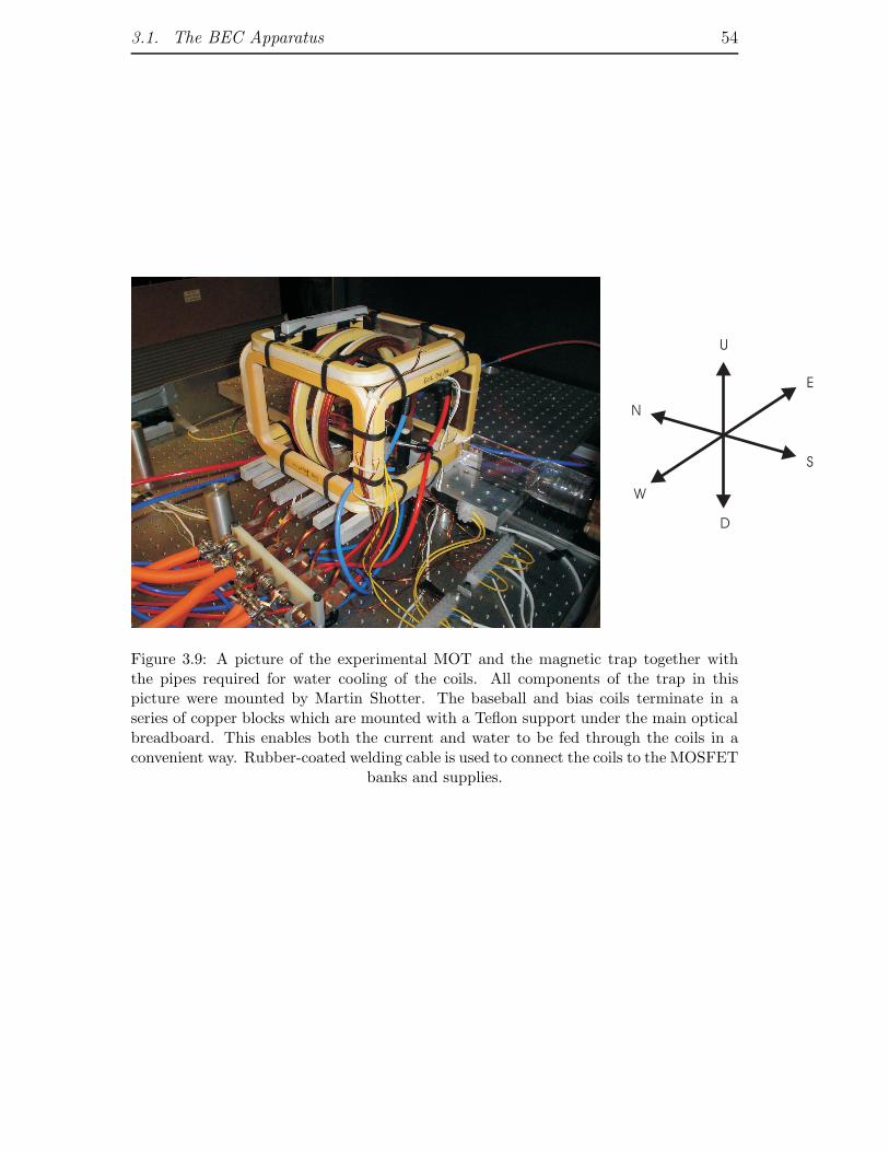
3.1. The BEC Apparatus 54
W
N
S
U
E
D
Figure 3.9: A picture of the experimental MOT and the magnetic trap together withthe pipes required for water cooling of the coils. All components of the trap in thispicture were mounted by Martin Shotter. The baseball and bias coils terminate in aseries of copper blocks which are mounted with a Teflon support under the main opticalbreadboard. This enables both the current and water to be fed through the coils in aconvenient way. Rubber-coated welding cable is used to connect the coils to the MOSFET
banks and supplies.
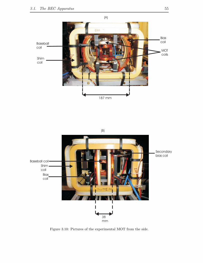
3.1. The BEC Apparatus 55
187 mm
Shim
coil
Baseball
coilMOT
coils
Bias
coil
Bias
coil
Shim
coil
Baseball coil
Secondary
bias coil
38
mm
(A)
(B)
Figure 3.10: Pictures of the experimental MOT from the side.
3.1. The BEC Apparatus 56
Transistor-Transistor Logic (TTL) inputs. Figures 3.9 and 3.10 are pictures of our
experimental MOT from various orientations.
Shim coils No. of turns Dimensions (mm) Separation (mm)E/W 67 196 × 138 226N/S 68 196 × 138 192U/D 68 (up); 67 (down) 196 × 196 167
Shim coils are required to null out any ambient magnetic fields, which is especially
vital for the optical molasses stage. They also move the centre of the MOT for
loading into the magnetic trap in the CMOT stage. The shim coils are six coils
mounted in a cuboid arrangement wound with 1 mm diameter wire. They are
labelled the U/D shims, E/W shims and N/S shims (specifications given in the
table above). All the shim coils were wound by Tony Hickman in the Clarendon
Laboratory. Since all the coils are rather bulky, the separation is defined by the
distance between the centres of the coil units. Like the MOT coils, the current
through the shim coils is controlled by a FET and the gate voltage for the FET
is provided by the multiplexer circuit. For every pair of shim coils, a maximum of
5 Amperes can flow through the wire to give a maximum field of 10 Gauss at the
centre of the geometry. In addition to nulling the magnetic field of the earth for
the molasses stage, the E/W shim coils are also used to provide a field that defines
the quantization axis for optical pumping and probing.
3.1.7 Magnetic trap
Construction
The baseball magnetic trap used in the experiment is a type of Ioffe-Pritchard
trap and it needs to fulfill certain geometry requirements to give confinement in
all three dimensions. The geometry of our baseball trap was modelled on that
of the previous baseball trap used in caesium experiments now taken to Durham
University by Simon Cornish. To calculate the fields in this trap, we simulated
the magnetic trapping potential using MATHEMATICA and the Biot-Savart law.
We wound the coils as close as possible to the vacuum chamber to provide the
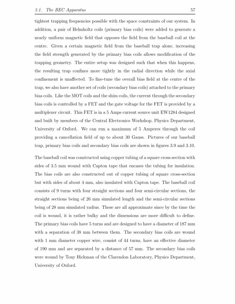
3.1. The BEC Apparatus 57
tightest trapping frequencies possible with the space constraints of our system. In
addition, a pair of Helmholtz coils (primary bias coils) were added to generate a
nearly uniform magnetic field that opposes the field from the baseball coil at the
centre. Given a certain magnetic field from the baseball trap alone, increasing
the field strength generated by the primary bias coils allows modification of the
trapping geometry. The entire setup was designed such that when this happens,
the resulting trap confines more tightly in the radial direction while the axial
confinement is unaffected. To fine-tune the overall bias field at the centre of the
trap, we also have another set of coils (secondary bias coils) attached to the primary
bias coils. Like the MOT coils and the shim coils, the current through the secondary
bias coils is controlled by a FET and the gate voltage for the FET is provided by a
multiplexer circuit. This FET is in a 5 Amps current source unit EW1284 designed
and built by members of the Central Electronics Workshop, Physics Department,
University of Oxford. We can run a maximum of 5 Amperes through the coil
providing a cancellation field of up to about 30 Gauss. Pictures of our baseball
trap, primary bias coils and secondary bias coils are shown in figures 3.9 and 3.10.
The baseball coil was constructed using copper tubing of a square cross-section with
sides of 3.5 mm wound with Capton tape that encases the tubing for insulation.
The bias coils are also constructed out of copper tubing of square cross-section
but with sides of about 4 mm, also insulated with Capton tape. The baseball coil
consists of 9 turns with four straight sections and four semi-circular sections, the
straight sections being of 26 mm simulated length and the semi-circular sections
being of 28 mm simulated radius. These are all approximate since by the time the
coil is wound, it is rather bulky and the dimensions are more difficult to define.
The primary bias coils have 5 turns and are designed to have a diameter of 187 mm
with a separation of 38 mm between them. The secondary bias coils are wound
with 1 mm diameter copper wire, consist of 44 turns, have an effective diameter
of 190 mm and are separated by a distance of 57 mm. The secondary bias coils
were wound by Tony Hickman of the Clarendon Laboratory, Physics Department,
University of Oxford.
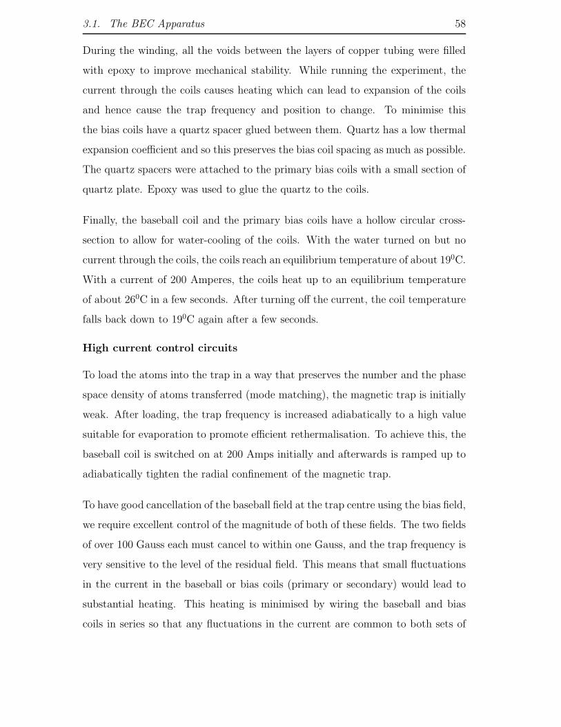
3.1. The BEC Apparatus 58
During the winding, all the voids between the layers of copper tubing were filled
with epoxy to improve mechanical stability. While running the experiment, the
current through the coils causes heating which can lead to expansion of the coils
and hence cause the trap frequency and position to change. To minimise this
the bias coils have a quartz spacer glued between them. Quartz has a low thermal
expansion coefficient and so this preserves the bias coil spacing as much as possible.
The quartz spacers were attached to the primary bias coils with a small section of
quartz plate. Epoxy was used to glue the quartz to the coils.
Finally, the baseball coil and the primary bias coils have a hollow circular cross-
section to allow for water-cooling of the coils. With the water turned on but no
current through the coils, the coils reach an equilibrium temperature of about 190C.
With a current of 200 Amperes, the coils heat up to an equilibrium temperature
of about 260C in a few seconds. After turning off the current, the coil temperature
falls back down to 190C again after a few seconds.
High current control circuits
To load the atoms into the trap in a way that preserves the number and the phase
space density of atoms transferred (mode matching), the magnetic trap is initially
weak. After loading, the trap frequency is increased adiabatically to a high value
suitable for evaporation to promote efficient rethermalisation. To achieve this, the
baseball coil is switched on at 200 Amps initially and afterwards is ramped up to
adiabatically tighten the radial confinement of the magnetic trap.
To have good cancellation of the baseball field at the trap centre using the bias field,
we require excellent control of the magnitude of both of these fields. The two fields
of over 100 Gauss each must cancel to within one Gauss, and the trap frequency is
very sensitive to the level of the residual field. This means that small fluctuations
in the current in the baseball or bias coils (primary or secondary) would lead to
substantial heating. This heating is minimised by wiring the baseball and bias
coils in series so that any fluctuations in the current are common to both sets of
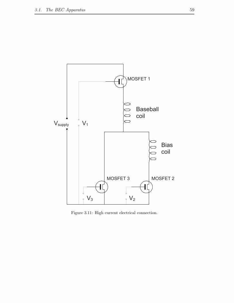
3.1. The BEC Apparatus 59
Baseballcoil
Biascoil
Vsupply
MOSFET 1
MOSFET 3 MOSFET 2
V1
V2V3
Figure 3.11: High current electrical connection.

3.1. The BEC Apparatus 60
coils. Figure 3.11 shows the electronics for control of the high current. The three
Metal Oxide Semiconductor Field-Effect Transistor (MOSFET) banks are labelled
MOSFET 1, MOSFET 2 and MOSFET 3. These MOSFETs work on the same
principle as FETs but we decided to use them to control higher currents. MOSFET
1 controls the overall current running through the entire setup, MOSFET 2 controls
the current through the path of the bias coil and MOSFET 3 controls the current
running through the bypass path. At the beginning of the experiment, MOSFET
1 is completely closed allowing 200 A of current to run through the baseball coil.
MOSFET 2 is either completely closed (when the experiment is run) or completely
open (at the end of the experiment or when it is not running). We control the
amount of current running through the bias coils by varying the gate voltage V3 of
MOSFET 3. For most of the experiment, V1 and V2 are constant. We change the
trapping geometry by changing V3.
In practice each MOSFET bank has 5 MOSFETs (STMicroelectronics STE180NE10)
connected in parallel and all linked to the same control voltage. Each MOSFET
has a current rating of 180 A and having five of them in each bank means each
bank is capable of taking in 900 A of current, well above what we need. The MOS-
FETs dissipate a considerable amount of heat and so are mounted on a copper
tube which is water cooled.
Current control electronics
In the following section, all signal names in inverted commas refer to the corre-
sponding input/output in Figure 3.12.
The magnetic trap current is controlled by two pairs of electronic circuits; a ‘Refer-
ence Voltage Board’ and ‘Main Feedback Board’ (see Figure 3.12). The ‘Reference
Voltage Board’ controls the trap turn on/off (and fast input control etc) and gener-
ates the input voltage for the ‘Main Feedback Board’. The ‘Main Feedback Board’
provides the gate voltage for the FET’s and the integrator part of the circuit reg-
ulates the current through the baseball and bias coils. The ‘Trap on/off TTL’ is
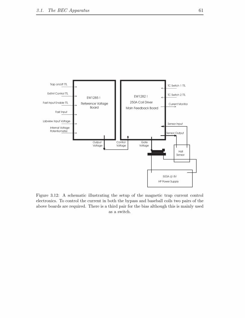
3.1. The BEC Apparatus 61
EW1285 !
Reference Voltage
Board
EW1282 !
250A Coil Driver
Main Feedback Board
Labview Input Voltage
Trap on/off TTL
Ext/Int Control TTL
Fast Input Enable TTL
Fast Input
Internal Voltage
Potentiometer
Output
Voltage
Control
Voltage
Gate
Voltage
TC Switch 1 TTL
TC Switch 2 TTL
Current Monitor
Sensor Input
Sensor Output
Hall
Sensor
500A @ 8V
HP Power Supply
Figure 3.12: A schematic illustrating the setup of the magnetic trap current controlelectronics. To control the current in both the bypass and baseball coils two pairs of theabove boards are required. There is a third pair for the bias although this is mainly used
as a switch.
3.1. The BEC Apparatus 62
controlled by a TTL signal. When it is set to high, the trap turns on to a level
set by the analogue ‘LabVIEW Input Voltage’. For a rapid turn on the trap is ini-
tially turned on without involving the feedback circuit in EW1282. The capacitors
are then switched back into the circuit to improve DC stability. For fast current
control the fast input facility can be used. The ‘Fast Input Enable TTL’ requires
a TTL signal in order to switch an extra reference voltage into the circuit. The
extra reference voltage is an analogue voltage applied to the ‘Fast Input’, and is
then summed into the circuit. This facility is required as the analogue input from
Labview is filtered (the ‘fast input’ is summed into the circuit after the filter) and
therefore fast current changes cannot be implemented.
For current stabilization and monitoring the welding cable (50 mm2 cross sectional
area) is passed through two closed loop current sensors (Honeywell CSNJ481) for
the baseball coil and the bypass welding cable. The current loop sensor consists
of a coil of 2000 turns wound around a ferrite core which circles the welding cable.
The Hall sensor maintains a condition of zero magnetic flux through the core by
balancing the current in the 2000 turn coil to cancel that from the cable. This cur-
rent is the output of the sensor and goes to the control electronics boards where it is
converted to an input voltage via a shunt resistor. This input is part of a feedback
mechanism in the ‘Main Feedback Board’ which generates and controls the current
in the Hall sensor. The ‘Current Monitor’ outputs for the baseball coil and the
bypass are plugged into a digital oscilloscope and this signal we monitor everyday
when running the experiment so any unusual behaviour would show immediately.
To check the stability of the high current, the ’Current Monitor’ outputs are con-
nected to a 6 d.p. precision DVM (Agilent 34401A - 6 1/2 Digit Multimeter) where
field fuctuations as small as a few mG can be observed. We ran the experiment
several times (the duration of each is about five minutes) and we found that the
variation of the current is comparable to the documented measurement error of
the DVM itself. From this we conclude that the current is sufficiently stable and
that the boards are functioning well. In normal operating conditions, the baseball
coil current is turned on to 200 A in about 1 ms and switches off even faster.
3.2. Dipole trap apparatus 63
Safety features
Safety measures were installed in the experiment to prevent the coils getting too
hot. K-type thermocouples were embedded in the baseball coil and one bias coil,
and on the surface of one MOT coil. These allow the temperature of the coils to be
read either directly with a thermocouple reader, or by interfacing to the computer.
The LabVIEW program that controls the experiment was then programmed such
that the experiment will not run if the temperature of any of the coils is higher
than 300C. In addition to that, alongside the thermocouples on these three coils,
thermistors were also placed. These are linked to a temperature interlock box in
which thermostat circuits (Cebek I-8) trip a relay when the temperature of the
thermistors rises above a certain value. The trip temperature of the circuit is set
around 550C.
3.1.8 Evaporation
The radio-frequencies required for evaporation were generated by a synthesized
function generator (Stanford DS345). The generator is capable of frequencies from
DC to 30 MHz and an amplitude up to a maximum of 10 Vpp (or 24 dBm)and the
signal generated is transmitted to the atoms via a two-turn coil. For impedance
matching between the load and the source, an effective 50 Ω resistor was placed
in series with the coil and this effective 50 Ω resistor was made by connecting
three 150 Ω resistors in parallel. Each of these resistors has a power rating of 2
Watts which means having three of these in parallel can take up to a maximum RF
power of 6 Watts. The evaporation ramps were calculated in Labview and then
transferred continuously to the frequency generator via the GPIB interface.
3.2 Dipole trap apparatus
This section describes the additional apparatus required for the experiments we
plan to do with the BEC. Parts of this section are based on reports of undergradu-
ate students Peter Baranowski and James Zacks who worked towards building some

3.2. Dipole trap apparatus 64
Verdi
V10
Coherent
MBR-110
l/2AOM
Figure 3.13: The laser system for dipole trapping.
components of the apparatus in our laboratory [64]. Where applicable, figures will
be referenced.
3.2.1 Lasers
Figure 3.13 shows the arrangement of the apparatus that generates the dipole
trapping beam. The Verdi V10 laser outputs a 532nm wavelength beam with a
maximum possible power of 10 Watts. The Verdi laser pumps a Coherent MBR-
110 Titanium-doped Sapphire laser that can be tuned between wavelengths 750
nm and 900 nm; we use a fixed wavelength of 830 nm at which a maximum output
power of 900 mW is available for our dipole trapping experiments.
Immediately after the Ti:Sapphire laser, we have a green filter which removes most
of the residue Verdi beam which comes through. After that, a lens of 10 cm fo-
cal length focuses the light into an AOM (Crystal Technology 3080-122) which
controls the output beam power passing onto the rest of the system. Immediately
after the AOM, we have a variable wave-plate in the form of a Babinet-Soleil Com-
pensator tuned to be a half-wave plate for our beam wavelength and a 25 cm focal
length lens to collimate the light. The beam then enters a polarisation-preserving
3.2. Dipole trap apparatus 65
fibre (OZ optics LPC-02-830-5/125/P-2.4.11AS-40-1A-3-5+LPC-08-830-5/125-P-
6.6-30AGR-40-1A-3-5) which acts as a good spatial filter. The pigtail collimator
which the dipole trapping beam leaves through consists of a diffraction limited
gradient index (grin) lens with a focal length of 30 mm. This gives a 1/e-diameter
of the collimated beam of ≈ 3.9 mm.
3.2.2 Acousto-Optic Deflector
The AOD is an ISOMET LS110A-830XY Dual Axis AO Deflector with two single
axis TeO2 deflectors orthogonally mounted. The deflectors work by diffracting the
light on acoustic waves generated in the crystal through the application of radio
frequencies. The centre frequency for this AOD is 50 MHz and it has a bandwidth
of 25 MHz, which gives a scan angle of 1.90 per axis. As shown in Figure 3.15 (A),
the optical axis is defined as the diffracted beam at central frequency νcentre=50
MHz. Two telescopic stages shown in Figure 3.15 (B) are placed between the AOD
and the four-lens objective to increase the beam diameter. This is so that we can
achieve a tighter spot size after focussing which results in a tighter dipole trap.
These telescopic stages achieve a magnification of m = f2·f4
f1·f3
= 3.75. The scanning
angle is therefore demagnified by the same factor.
The beam diameter needs to be increased and the beams have to be as collimated
as possible after the last stage. This is done by choosing appropriate lens pairs and
setting the distance between each two lenses that form a telescope to the sum of
their focal lengths. Also, the deflector output aperture and the first focal plane of
the focusing objective have to be conjugate points. This is achieved by setting the
lenses up as shown in Figure 3.15 (B). Therefore the distance between the deflector
and the 4-lens objective is fixed to 3.8 m. Finally, the aberrations introduced by
the telescopes need to be small so we chose lenses with large focal lengths. Figure
3.16 shows the temporary configuration of the electronics we used to manipulate
the dipole beam. In the near future we hope to replace this by a more robust
system.

3.2. Dipole trap apparatus 66
AOD
To next
optical
bench
f=400 mm
f=250 mmf=500 mm
f=750 mm
Science
cell
Four-lens
objective
(A)
(B)
l/4
Figure 3.14: The optics around the Acousto-Optic Deflector (AOD). (A) shows thecomponents on the same optical bench as the apparatus shown in Figure 3.1. (B) showshow the dipole trapping beam is elevated to the MOT using a periscope before reflectingfrom more mirrors to get to the vacuum cell. The λ/4 plate after the AOD is to convert
circularly-polarised diffracted light off the AOD back to linearly polarised light.
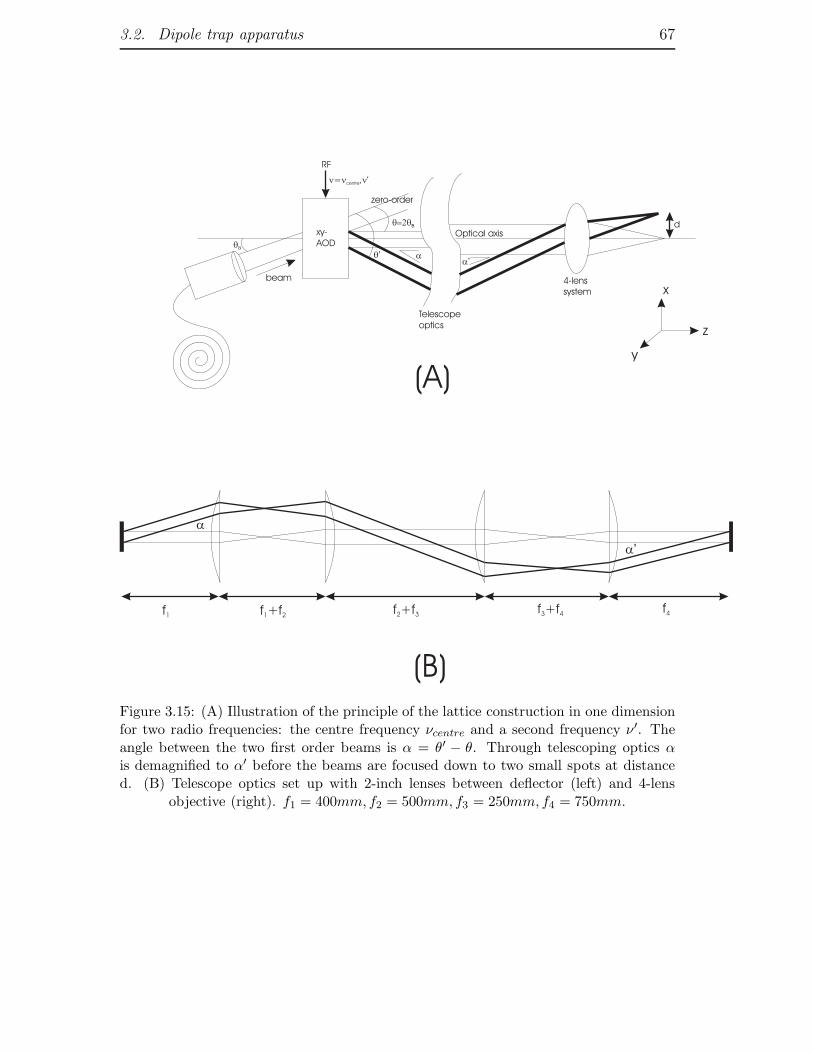
3.2. Dipole trap apparatus 67
a
a’
f1 f +f1 2f +f2 3
f +f3 4f4
q=2qB
q’ aqB
a’
d
Telescope
optics
4-lens
system
xy-
AOD
RF
n n n= , ’centre
Optical axis
zero-order
beam
(A)
(B)
y
z
x
Figure 3.15: (A) Illustration of the principle of the lattice construction in one dimensionfor two radio frequencies: the centre frequency νcentre and a second frequency ν ′. Theangle between the two first order beams is α = θ′ − θ. Through telescoping optics αis demagnified to α′ before the beams are focused down to two small spots at distanced. (B) Telescope optics set up with 2-inch lenses between deflector (left) and 4-lens
objective (right). f1 = 400mm, f2 = 500mm, f3 = 250mm, f4 = 750mm.

3.2. Dipole trap apparatus 68
Arbitrary
waveform
generator
RF
splitter
RF mixer RF mixer
Signal
generator
Signal
generator
AOD
x
y
RF
amplifier
RF
amplifier
Figure 3.16: Temporary schematic for the electronics required for beam spot manipu-lation. The arbitrary waveform generator was a HP8770A AWG. The signal generatorswere Agilent 33220A and the RF splitters were MINICIRCUITS ZFSC-2-1W. The am-
plifiers were MINICIRCUITS ZHL-1-2W and the RF mixers were HP 10534A.
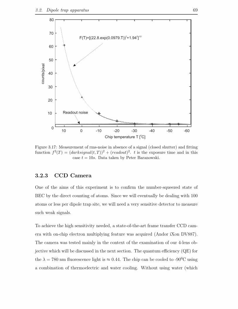
3.2. Dipole trap apparatus 69
10
20
counts
/pix
el
0
30
40
50
60
70
80
Chip temperature T [ C]0
Readout noise
10 0 -10 -20 -30 -40 -50 -60
F(T)=[(22.8.exp(0.0979.T)) +1.94 ]2 2 1/2
Figure 3.17: Measurement of rms-noise in absence of a signal (closed shutter) and fittingfunction f2(T ) = (darksignal(t, T ))2 + (readout)2. t is the exposure time and in this
case t = 10s. Data taken by Peter Baranowski.
3.2.3 CCD Camera
One of the aims of this experiment is to confirm the number-squeezed state of
BEC by the direct counting of atoms. Since we will eventually be dealing with 100
atoms or less per dipole trap site, we will need a very sensitive detector to measure
such weak signals.
To achieve the high sensitivity needed, a state-of-the-art frame transfer CCD cam-
era with on-chip electron multiplying feature was acquired (Andor iXon DV887).
The camera was tested mainly in the context of the examination of our 4-lens ob-
jective which will be discussed in the next section. The quantum efficiency (QE) for
the λ = 780 nm fluorescence light is ≈ 0.44. The chip can be cooled to -900C using
a combination of thermoelectric and water cooling. Without using water (which
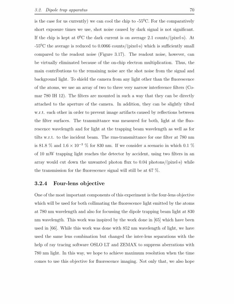
3.2. Dipole trap apparatus 70
is the case for us currently) we can cool the chip to -550C. For the comparatively
short exposure times we use, shot noise caused by dark signal is not significant.
If the chip is kept at 00C the dark current is on average 2.1 counts/(pixel·s). At
-550C the average is reduced to 0.0066 counts/(pixel·s) which is sufficiently small
compared to the readout noise (Figure 3.17). The readout noise, however, can
be virtually eliminated because of the on-chip electron multiplication. Thus, the
main contributions to the remaining noise are the shot noise from the signal and
background light. To shield the camera from any light other than the fluorescence
of the atoms, we use an array of two to three very narrow interference filters (Co-
mar 780 IH 12). The filters are mounted in such a way that they can be directly
attached to the aperture of the camera. In addition, they can be slightly tilted
w.r.t. each other in order to prevent image artifacts caused by reflections between
the filter surfaces. The transmittance was measured for both, light at the fluo-
rescence wavelength and for light at the trapping beam wavelength as well as for
tilts w.r.t. to the incident beam. The rms-transmittance for one filter at 780 nm
is 81.8 % and 1.6 × 10⁻³ % for 830 nm. If we consider a scenario in which 0.1 %
of 10 mW trapping light reaches the detector by accident, using two filters in an
array would cut down the unwanted photon flux to 0.04 photons/(pixel·s) while
the transmission for the fluorescence signal will still be at 67 %.
3.2.4 Four-lens objective
One of the most important components of this experiment is the four-lens objective
which will be used for both collimating the fluorescence light emitted by the atoms
at 780 nm wavelength and also for focussing the dipole trapping beam light at 830
nm wavelength. This work was inspired by the work done in [65] which have been
used in [66]. While this work was done with 852 nm wavelength of light, we have
used the same lens combination but changed the inter-lens separations with the
help of ray tracing software OSLO LT and ZEMAX to suppress aberrations with
780 nm light. In this way, we hope to achieve maximum resolution when the time
comes to use this objective for fluorescence imaging. Not only that, we also hope
3.2. Dipole trap apparatus 71
1 2 3 4
S1 S2 S3 S418 mm
15 mm
12.75mm
11.75mm
1 7/16” thread, 20 tpi
Threaded holding ring
Lenses: Aluminium spacers:
1: LPV25/-75 3:LPX25/100 S1: 6.0 mm S3: 2.77 mm2: LPX25/100 4:Custom meniscus Lens S2: 5.82 mm S4: 3.08 mm
a b c d e f g h i j
R1 R2 R3 R4 R5 R6 R7 R8
(a)
(b)
37 mm
Figure 3.18: Construction scheme. Designed, constructed and tested by Peter Bara-nowski and James Zacks. In (b), the lens surface curvatures are (in mm): R1flat,R2 =39.08, R3 = 103.29, R4 = −103.29, R5 = 39.08, R6flat,R7 = 26.00, R8=78.16. Thewidths of the lenses and air gaps are (in mm): a=3.08, b=7.24, c=4.97, d=0.40, e=5.12,f =0.40, g=5.07, h=21.00, i (silica)=2.00, j=12.73. All lenses have a diameter of 25.4
mm.

3.3. Diagnostics 72
to attain very small spot sizes for 830 nm wavelength dipole trapping light for a
deep dipole trap. The lenses were arranged within a brass tube and separated by
aluminium spacers. The tube was then mounted on a five-axis translation stage (X,
Y, Z, pitch and yaw) for ease of alignment. The final dimensions of the objective
are shown in Figure 3.18.
To simulate real conditions, the simulations done in [64] also take into account the
vacuum glass cell window of 2 mm thickness since it will also introduce spherical
aberrations and thus act as an effective lens. Results show that the diffraction
limit of this system was 1.74 µm and that the simulated rms spot size given by
this system provided that the entire aperture size was used was < 0.5 µm (diffrac-
tion limited performance). Given this diffraction limited performance rather than
aberration limited, we apply Rayleigh’s criterion which gives the smallest resolv-
able distance ∆l as
∆l = 1.22fλ
D(3.1)
where f is the effective focal length of the system, λ is the wavelength of the light
used and D is the diameter of the aperture. In our case, f=37 mm, D=23.5 mm
and λ= 780 nm which gives ∆l= 1.74 µm. The effective numerical aperture of the
system was NA=0.27.
3.3 Diagnostics
3.3.1 Recapture method
Fluorescence light from a MOT cloud is used to monitor the number of atoms for
diagnostic purposes. A collection lens is placed as close as possible to the MOT
behind which we have a photodiode placed at the point at which the collected
light is focussed. The relevant calculations required to determine approximately
the number of atoms in the cloud is given in later chapters but comparison of
fluorescence signals is important so that we run the experiment each day under
the same conditions.
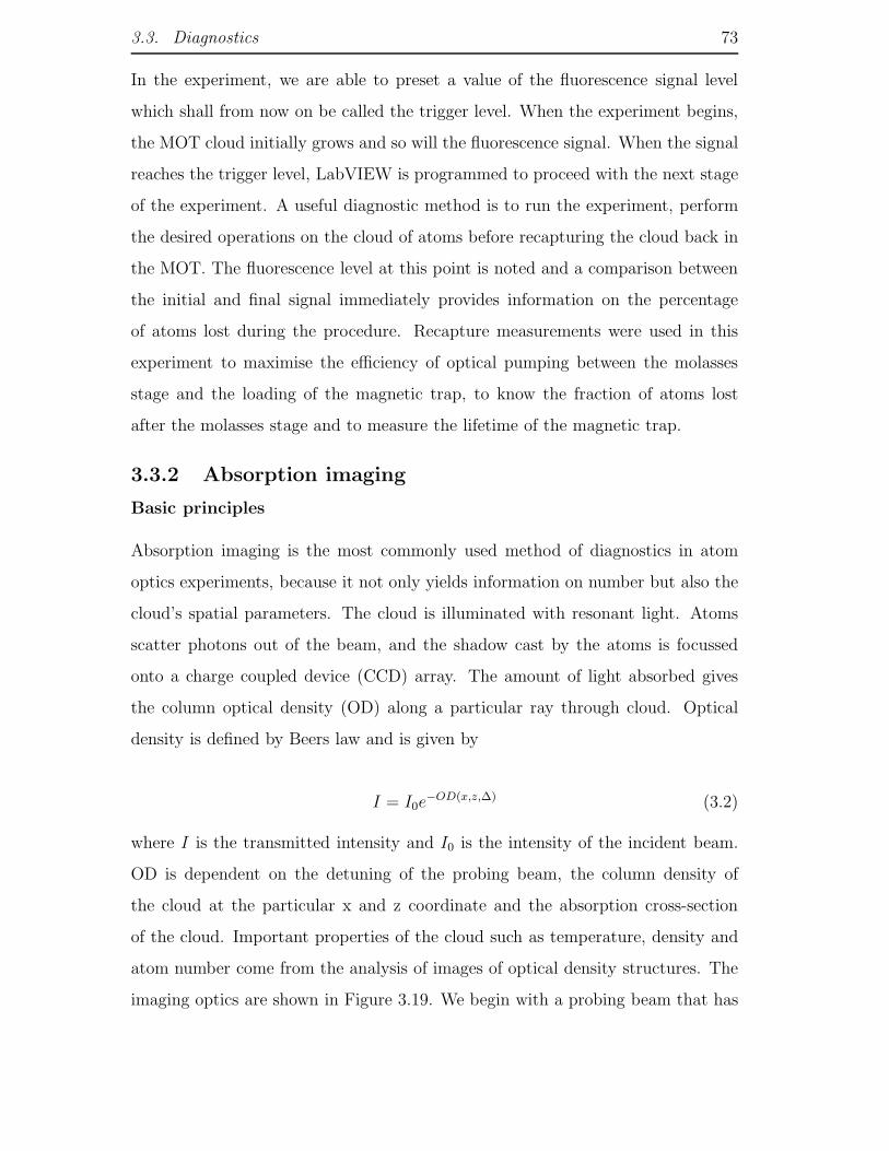
3.3. Diagnostics 73
In the experiment, we are able to preset a value of the fluorescence signal level
which shall from now on be called the trigger level. When the experiment begins,
the MOT cloud initially grows and so will the fluorescence signal. When the signal
reaches the trigger level, LabVIEW is programmed to proceed with the next stage
of the experiment. A useful diagnostic method is to run the experiment, perform
the desired operations on the cloud of atoms before recapturing the cloud back in
the MOT. The fluorescence level at this point is noted and a comparison between
the initial and final signal immediately provides information on the percentage
of atoms lost during the procedure. Recapture measurements were used in this
experiment to maximise the efficiency of optical pumping between the molasses
stage and the loading of the magnetic trap, to know the fraction of atoms lost
after the molasses stage and to measure the lifetime of the magnetic trap.
3.3.2 Absorption imaging
Basic principles
Absorption imaging is the most commonly used method of diagnostics in atom
optics experiments, because it not only yields information on number but also the
cloud’s spatial parameters. The cloud is illuminated with resonant light. Atoms
scatter photons out of the beam, and the shadow cast by the atoms is focussed
onto a charge coupled device (CCD) array. The amount of light absorbed gives
the column optical density (OD) along a particular ray through cloud. Optical
density is defined by Beers law and is given by
I = I0e−OD(x,z,∆) (3.2)
where I is the transmitted intensity and I0 is the intensity of the incident beam.
OD is dependent on the detuning of the probing beam, the column density of
the cloud at the particular x and z coordinate and the absorption cross-section
of the cloud. Important properties of the cloud such as temperature, density and
atom number come from the analysis of images of optical density structures. The
imaging optics are shown in Figure 3.19. We begin with a probing beam that has

3.3. Diagnostics 74
Andor
iXon
Doublet
f=80 mm
l/4
Doublet
f=125 mm
Doublet
f=315 mm
Atoms
Figure 3.19: Schematic of the imaging setup for observation of condensate. For a mag-nification of unity, we use two f=200 mm singlet lenses.

3.3. Diagnostics 75
already been spatially filtered using a single-mode polarisation-preserving optical
fibre. The probe beam is then allowed to expand before being collimated by a
doublet lens of focal length 80 mm. The collimated beam was measured to have
a 1/e radius of 4.6 mm. There is a quarter-wave plate placed after the lens to
make the probing beam circularly-polarised which is desirable because it drives
the atoms on a cycling transition in the probing process and thus gives a good
signal-to-noise ratio. For equation 3.2 to hold true, we want a low intensity for
our probe beam. Therefore, we set the intensity of the beam to be one-tenth
the saturation intensity of the probing transition. For the current beam size, this
requires the total beam power to be 100 µW and we monitor this occasionally to
achieve this intensity. For observation of condensates, we want a magnification of
around 2.5 and this was done using two doublet lenses of focal lengths 125 mm
and 315 mm. The distance between the cloud of atoms and the first lens after the
science cell is 125 mm and the distance between the second doublet lens and the
CCD chip is 315 mm.
To image the atoms, the current in the magnetic trap coils is turned off in less
than 10 µs and the atoms are pumped into the F = 2 sublevel with a 200 µs pulse
of light resonant with the 5S1/2;F = 1 −→ 5P3/2;F′ = 2 transition (repumping
transition). The cloud is then probed by applying a 200µs pulse of circularly
polarized light resonant with the 5S1/2;F = 2 −→ 5P3/2;F′ = 3 transition. An
AOM is used for fast shuttering of the probe light. The shadow of the atoms in the
beam is then imaged onto a CCD array. Our CCD camera is a front-illuminated
CCD array with pixels of dimensions 16× 16µm. The entire array was 512 × 512
pixels. The quantum efficiency at 780 nm peaks at 43% and the readout noise is
62 electrons per pixel in the fastest readout mode of 10 MHz. The camera feeds
on an edge trigger and sometimes electrical noise around the laboratory cause the
camera to take pictures unexpectedly. To minimise this, the trigger level sent to
the camera is set to high first until moments before an image was taken at which
point the TTL logic level is set to low for a typical length of 15 ms before it is set
to high which triggers the camera to take an image.
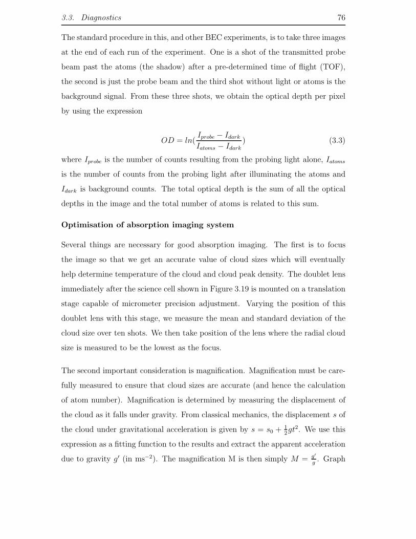
3.3. Diagnostics 76
The standard procedure in this, and other BEC experiments, is to take three images
at the end of each run of the experiment. One is a shot of the transmitted probe
beam past the atoms (the shadow) after a pre-determined time of flight (TOF),
the second is just the probe beam and the third shot without light or atoms is the
background signal. From these three shots, we obtain the optical depth per pixel
by using the expression
OD = ln(Iprobe − Idark
Iatoms − Idark
) (3.3)
where Iprobe is the number of counts resulting from the probing light alone, Iatoms
is the number of counts from the probing light after illuminating the atoms and
Idark is background counts. The total optical depth is the sum of all the optical
depths in the image and the total number of atoms is related to this sum.
Optimisation of absorption imaging system
Several things are necessary for good absorption imaging. The first is to focus
the image so that we get an accurate value of cloud sizes which will eventually
help determine temperature of the cloud and cloud peak density. The doublet lens
immediately after the science cell shown in Figure 3.19 is mounted on a translation
stage capable of micrometer precision adjustment. Varying the position of this
doublet lens with this stage, we measure the mean and standard deviation of the
cloud size over ten shots. We then take position of the lens where the radial cloud
size is measured to be the lowest as the focus.
The second important consideration is magnification. Magnification must be care-
fully measured to ensure that cloud sizes are accurate (and hence the calculation
of atom number). Magnification is determined by measuring the displacement of
the cloud as it falls under gravity. From classical mechanics, the displacement s of
the cloud under gravitational acceleration is given by s = s0 + 12gt2. We use this
expression as a fitting function to the results and extract the apparent acceleration
due to gravity g′ (in ms−2). The magnification M is then simply M = g′
g. Graph

3.3. Diagnostics 77
(A)
(B)
-6 -4 -2 0 2 4 6 8 10 12 14
1
2
3
4
5
6
7
8
N/*1
06
Probe beam detuning / MHz
Figure 3.20: Characterisation of absorption imaging. (A) shows measurement of magni-fication where the cloud position has been converted from pixels to microns. (B) showsa scan of detuning to ensure that the probing beam frequency is on resonance with the
F = 2 −→ F ′ = 3 transition.
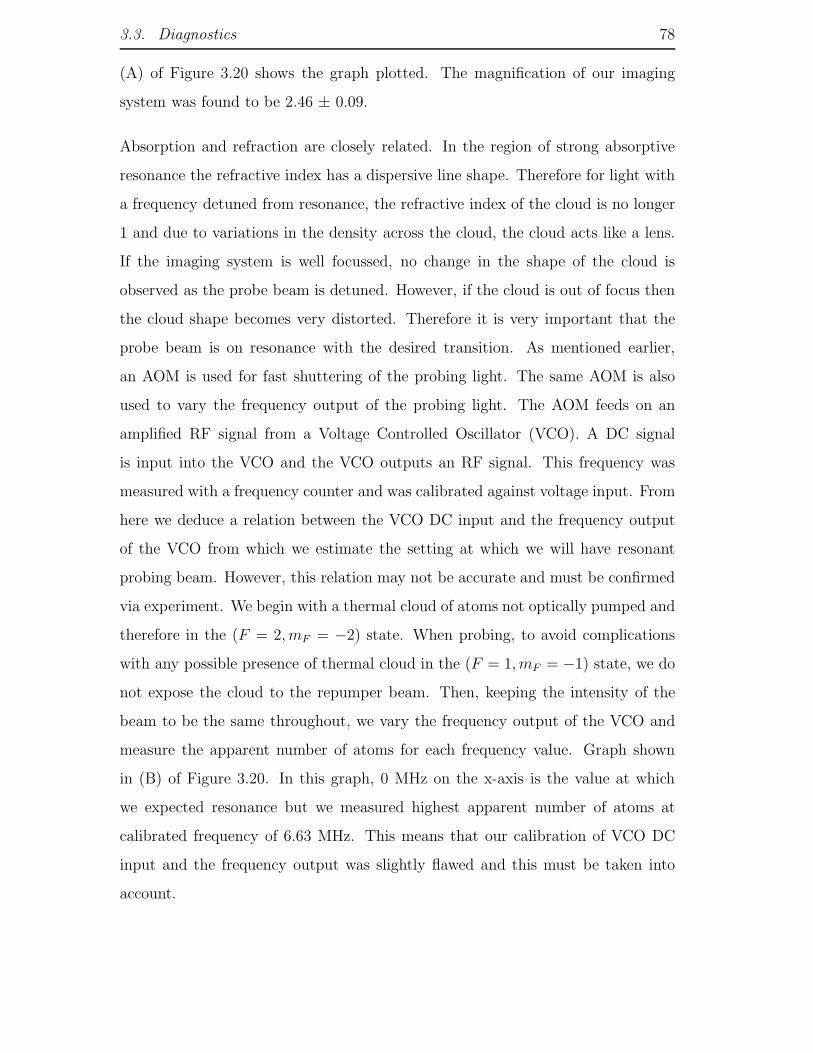
3.3. Diagnostics 78
(A) of Figure 3.20 shows the graph plotted. The magnification of our imaging
system was found to be 2.46 ± 0.09.
Absorption and refraction are closely related. In the region of strong absorptive
resonance the refractive index has a dispersive line shape. Therefore for light with
a frequency detuned from resonance, the refractive index of the cloud is no longer
1 and due to variations in the density across the cloud, the cloud acts like a lens.
If the imaging system is well focussed, no change in the shape of the cloud is
observed as the probe beam is detuned. However, if the cloud is out of focus then
the cloud shape becomes very distorted. Therefore it is very important that the
probe beam is on resonance with the desired transition. As mentioned earlier,
an AOM is used for fast shuttering of the probing light. The same AOM is also
used to vary the frequency output of the probing light. The AOM feeds on an
amplified RF signal from a Voltage Controlled Oscillator (VCO). A DC signal
is input into the VCO and the VCO outputs an RF signal. This frequency was
measured with a frequency counter and was calibrated against voltage input. From
here we deduce a relation between the VCO DC input and the frequency output
of the VCO from which we estimate the setting at which we will have resonant
probing beam. However, this relation may not be accurate and must be confirmed
via experiment. We begin with a thermal cloud of atoms not optically pumped and
therefore in the (F = 2, mF = −2) state. When probing, to avoid complications
with any possible presence of thermal cloud in the (F = 1, mF = −1) state, we do
not expose the cloud to the repumper beam. Then, keeping the intensity of the
beam to be the same throughout, we vary the frequency output of the VCO and
measure the apparent number of atoms for each frequency value. Graph shown
in (B) of Figure 3.20. In this graph, 0 MHz on the x-axis is the value at which
we expected resonance but we measured highest apparent number of atoms at
calibrated frequency of 6.63 MHz. This means that our calibration of VCO DC
input and the frequency output was slightly flawed and this must be taken into
account.
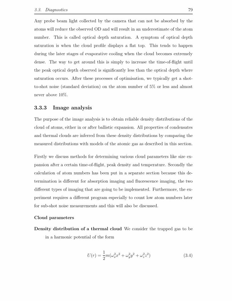
3.3. Diagnostics 79
Any probe beam light collected by the camera that can not be absorbed by the
atoms will reduce the observed OD and will result in an underestimate of the atom
number. This is called optical depth saturation. A symptom of optical depth
saturation is when the cloud profile displays a flat top. This tends to happen
during the later stages of evaporative cooling when the cloud becomes extremely
dense. The way to get around this is simply to increase the time-of-flight until
the peak optical depth observed is significantly less than the optical depth where
saturation occurs. After these processes of optimisation, we typically get a shot-
to-shot noise (standard deviation) on the atom number of 5% or less and almost
never above 10%.
3.3.3 Image analysis
The purpose of the image analysis is to obtain reliable density distributions of the
cloud of atoms, either in or after ballistic expansion. All properties of condensates
and thermal clouds are inferred from these density distributions by comparing the
measured distributions with models of the atomic gas as described in this section.
Firstly we discuss methods for determining various cloud parameters like size ex-
pansion after a certain time-of-flight, peak density and temperature. Secondly the
calculation of atom numbers has been put in a separate section because this de-
termination is different for absorption imaging and fluorescence imaging, the two
different types of imaging that are going to be implemented. Furthermore, the ex-
periment requires a different program especially to count low atom numbers later
for sub-shot noise measurements and this will also be discussed.
Cloud parameters
Density distribution of a thermal cloud We consider the trapped gas to be
in a harmonic potential of the form
U(r) =1
2m(ω2
xx2 + ω2
yy2 + ω2
zz2) (3.4)
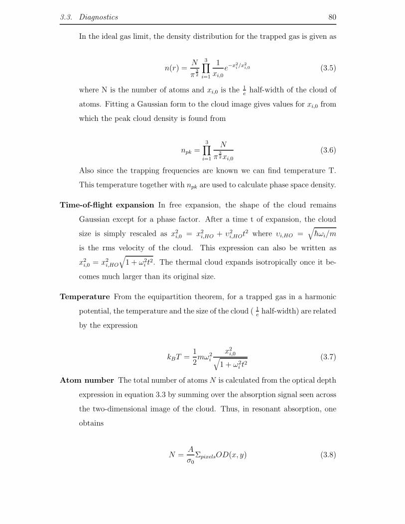
3.3. Diagnostics 80
In the ideal gas limit, the density distribution for the trapped gas is given as
n(r) =N
π3
2
3∏
i=1
1
xi,0
e−x2
i /x2
i,0 (3.5)
where N is the number of atoms and xi,0 is the 1e
half-width of the cloud of
atoms. Fitting a Gaussian form to the cloud image gives values for xi,0 from
which the peak cloud density is found from
npk =3∏
i=1
N
π3
2xi,0
(3.6)
Also since the trapping frequencies are known we can find temperature T.
This temperature together with npk are used to calculate phase space density.
Time-of-flight expansion In free expansion, the shape of the cloud remains
Gaussian except for a phase factor. After a time t of expansion, the cloud
size is simply rescaled as x2i,0 = x2
i,HO + υ2i,HOt
2 where υi,HO =√
hωi/m
is the rms velocity of the cloud. This expression can also be written as
x2i,0 = x2
i,HO
√
1 + ω2i t
2. The thermal cloud expands isotropically once it be-
comes much larger than its original size.
Temperature From the equipartition theorem, for a trapped gas in a harmonic
potential, the temperature and the size of the cloud ( 1e
half-width) are related
by the expression
kBT =1
2mω2
i
x2i,0
√
1 + ω2i t
2(3.7)
Atom number The total number of atoms N is calculated from the optical depth
expression in equation 3.3 by summing over the absorption signal seen across
the two-dimensional image of the cloud. Thus, in resonant absorption, one
obtains
N =A
σ0ΣpixelsOD(x, y) (3.8)
3.3. Diagnostics 81
where A is the effective pixel size after taking the magnification of the imaging
system into account and σ0 being the resonant absorption cross-section (σ0 =
2.91 × 10⁻⁹cm2). Take note that A=MA′ where M is magnification and A′
is the actual pixel area (A′=(16µm)2).
Chapter 4
Producing BEC
4.1 Loading the magnetic trap
The first step towards Bose-Einstein Condensation (BEC) is to optimise the loading
of atoms into the experimental MOT, i.e. load as many as atoms as possible into
the MOT quickly. To achieve this, there are various parameters associated with the
pyramidal MOT and the experimental MOT that were adjusted. The general aim
of the pyramidal MOT is to cool atoms from room temperature before these cooled
atoms are transferred to the science MOT via a small aperture in the pyramidal
setup. As a rule of thumb, being able to trap as many atoms as possible in the
pyramidal MOT would be a good start. As for the experimental MOT, ideally, we
would like to trap as many atoms as possible in a cold and dense cloud by having a
large magnetic gradient, high laser beam detuning and lots of cooling beam power.
However, our available laser beam power is limited and therefore we had to be
content with a reasonable magnetic gradient (10 G/cm) and laser beam detuning
in order to get a decent number of atoms. In addition to the parameters related to
the experimental MOT,we also varied the detuning of the cooling beam entering
the pyramidal MOT. This is because this detuning affects the density of our cloud
in the pyramidal MOT which affects the rate of atoms transferred through the
aperture.
82

4.1. Loading the magnetic trap 83
-3.5 -3.0 -2.5 -2.0 -1.5 -1.0 -0.5 0.0 0.5
0.0
0.2
0.4
0.6
0.8
1.0
N/*1
08
d G/
Figure 4.1: Optimization of the atom number in the pyramidal MOT. The dependenceof the atom number on laser frequency detuning (the trap light detuning is given in units
of δ/Γ where Γ is the natural decay rate of the excited level).
95 100 105 110 115 120 125 130 135
0
5
10
15
20
25
Position / mm
Po
we
r /
Wm
Figure 4.2: Measurement of the intensity profile of the laser beam going into the pyra-midal MOT

4.1. Loading the magnetic trap 84
4.1.1 Pyramidal MOT
The optimisation of capture rate of atoms in the pyramidal MOT leads to fast
loading of the experimental MOT. The only variable which we varied to optimise
this was the laser detuning with respect to the F = 2 −→ F ′ = 3 transition. The
number of atoms is determined from fluorescence measurements. A collection lens
of focal length 10 cm was placed at approximately 20.5 cm from the atoms collected
in the pyramid and a photodiode was placed at about 16 cm from the lens. The
collection lens has a clear aperture diameter of 6.2 cm when mounted. Figure 4.1
illustrates the dependence of the atoms captured in the pyramidal MOT on the
laser detuning. There was 3.2 mW of repumper beam power and 41.6 mW cooling
beam power at the time of measurement. The radius (1/e) of the cooling beam
was measured to be 11.9 mm and this was measured by translating a partially
closed iris across the beam and measuring the beam power transmitted through
the small aperture (1 mm diameter) presented by the iris. Figure 4.2 shows the
graph for this measurement. We ran 28 Amperes of current through the pyramidal
quadrupole coil to give a magnetic gradient of 14 Gcm−1.
4.1.2 Experimental MOT
This section describes the optimisation of the loading of the science MOT and
gives some results for its loading curve and lifetime.
The number of atoms in our MOT can be estimated given various parameters
like beam detuning, beam intensity and the amount of fluorescence light that the
atoms emit. We begin with a simple setup where we have a f=8 cm lens with an
effective aperture diameter of 2.3 cm placed about 16 cm away from the cloud of
atoms. This lens is the collection lens and the collected fluorescent light is then
focussed onto a photodiode. This photodiode has a responsitivity of 63.1 V/mW.
So given the photodiode signal which we observe with an oscilloscope, we know the
power of the light that falls on the photodiode, the solid angle presented by the
collection lens and therefore total light emitted by the cloud of atoms. From this
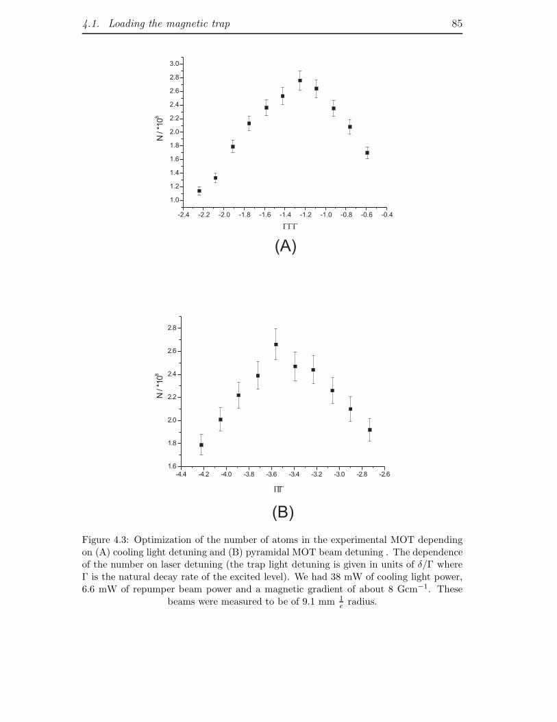
4.1. Loading the magnetic trap 85
-2.4 -2.2 -2.0 -1.8 -1.6 -1.4 -1.2 -1.0 -0.8 -0.6 -0.4
1.0
1.2
1.4
1.6
1.8
2.0
2.2
2.4
2.6
2.8
3.0
N/*1
08
???
-4.4 -4.2 -4.0 -3.8 -3.6 -3.4 -3.2 -3.0 -2.8 -2.6
1.6
1.8
2.0
2.2
2.4
2.6
2.8
N/*1
08
???
(A)
(B)
Figure 4.3: Optimization of the number of atoms in the experimental MOT dependingon (A) cooling light detuning and (B) pyramidal MOT beam detuning . The dependenceof the number on laser detuning (the trap light detuning is given in units of δ/Γ whereΓ is the natural decay rate of the excited level). We had 38 mW of cooling light power,6.6 mW of repumper beam power and a magnetic gradient of about 8 Gcm−1. These
beams were measured to be of 9.1 mm 1e radius.
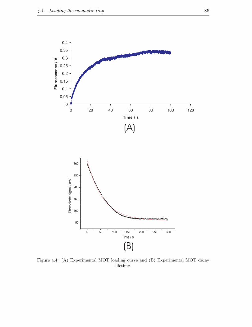
4.1. Loading the magnetic trap 86
0
0.05
0.1
0.15
0.2
0.25
0.3
0.35
0.4
0 20 40 60 80 100 120
Time / s
Flu
roescen
ce
/V
0 50 100 150 200 250 300
50
100
150
200
250
300
Photo
dio
de
signal/
mV
Time / s
(A)
(B)
Figure 4.4: (A) Experimental MOT loading curve and (B) Experimental MOT decaylifetime.

4.1. Loading the magnetic trap 87
information, we estimate the number of atoms in the cloud at the centre of our
MOT. The first objective was to optimise the loading rate by varying the frequency
detuning of the cooling beam and also of the pyramidal MOT beams. We then
make a comparison based on the signal observed on the oscilloscope after loading
for 10 seconds. It is assumed that the number of atoms attained in the MOT after
10 seconds is a good indicator of the eventual number of atoms. The results are
shown in Figure 4.3.
Figure 4.4 shows two other features of our MOT. The first graph shows the loading
curve. We attain approximately 2.8×10⁸ atoms in the first 10 seconds and we reach
equilibrium of about 6 × 10⁸ atoms after about 100 seconds. This means we have
an initial loading rate of about 2.8× 10⁷ atoms per second. As for the lifetime, we
fitted a standard exponential decay to the second graph and this yielded a lifetime
of 255 seconds which is slightly more than 4 minutes. These experiments are done
under the same conditions as those performed in Figure 4.3 but this time round
with a detuning of -10 MHz.
4.1.3 Compressed MOT and optical molasses
The MOT was optimised to load as many cold atoms as possible in the shortest
amount of time. However, the conditions that are best for loading give a cloud
of atoms that is too hot to transfer efficiently into a magnetic trap. Several more
processes are required to further cool down the atoms and give a significantly
higher density. They are the so-called Compressed MOT (CMOT) and the optical
molasses stage.
The CMOT stage serves two purposes: to increase phase-space density of the
cloud and also to match the centre of the MOT to the centre of the magnetic
trap. The current running through the shim coils is varied to move the centre of
the MOT so that it coincides with the centre of the magnetic trap. Initially, if
the cloud is not exactly at the centre of the magnetic trap, the cloud of atoms
undergoes an oscillation about the centre of the magnetic trap and this sloshing
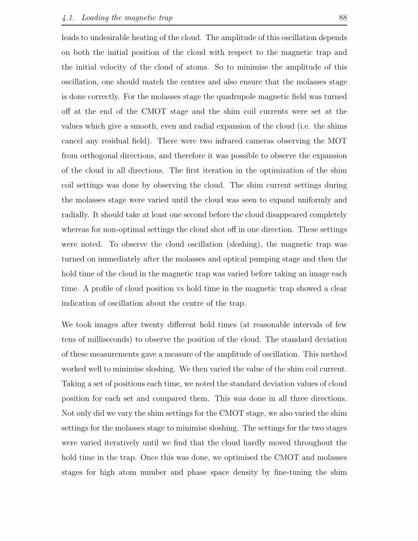
4.1. Loading the magnetic trap 88
leads to undesirable heating of the cloud. The amplitude of this oscillation depends
on both the initial position of the cloud with respect to the magnetic trap and
the initial velocity of the cloud of atoms. So to minimise the amplitude of this
oscillation, one should match the centres and also ensure that the molasses stage
is done correctly. For the molasses stage the quadrupole magnetic field was turned
off at the end of the CMOT stage and the shim coil currents were set at the
values which give a smooth, even and radial expansion of the cloud (i.e. the shims
cancel any residual field). There were two infrared cameras observing the MOT
from orthogonal directions, and therefore it was possible to observe the expansion
of the cloud in all directions. The first iteration in the optimization of the shim
coil settings was done by observing the cloud. The shim current settings during
the molasses stage were varied until the cloud was seen to expand uniformly and
radially. It should take at least one second before the cloud disappeared completely
whereas for non-optimal settings the cloud shot off in one direction. These settings
were noted. To observe the cloud oscillation (sloshing), the magnetic trap was
turned on immediately after the molasses and optical pumping stage and then the
hold time of the cloud in the magnetic trap was varied before taking an image each
time. A profile of cloud position vs hold time in the magnetic trap showed a clear
indication of oscillation about the centre of the trap.
We took images after twenty different hold times (at reasonable intervals of few
tens of milliseconds) to observe the position of the cloud. The standard deviation
of these measurements gave a measure of the amplitude of oscillation. This method
worked well to minimise sloshing. We then varied the value of the shim coil current.
Taking a set of positions each time, we noted the standard deviation values of cloud
position for each set and compared them. This was done in all three directions.
Not only did we vary the shim settings for the CMOT stage, we also varied the shim
settings for the molasses stage to minimise sloshing. The settings for the two stages
were varied iteratively until we find that the cloud hardly moved throughout the
hold time in the trap. Once this was done, we optimised the CMOT and molasses
stages for high atom number and phase space density by fine-tuning the shim
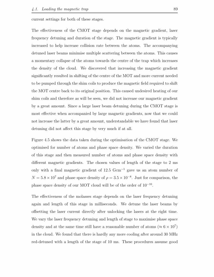
4.1. Loading the magnetic trap 89
current settings for both of these stages.
The effectiveness of the CMOT stage depends on the magnetic gradient, laser
frequency detuning and duration of the stage. The magnetic gradient is typically
increased to help increase collision rate between the atoms. The accompanying
detuned laser beams minimise multiple scattering between the atoms. This causes
a momentary collapse of the atoms towards the centre of the trap which increases
the density of the cloud. We discovered that increasing the magnetic gradient
significantly resulted in shifting of the centre of the MOT and more current needed
to be pumped through the shim coils to produce the magnetic field required to shift
the MOT centre back to its original position. This caused undesired heating of our
shim coils and therefore as will be seen, we did not increase our magnetic gradient
by a great amount. Since a large laser beam detuning during the CMOT stage is
most effective when accompanied by large magnetic gradients, now that we could
not increase the latter by a great amount, understandable we have found that laser
detuning did not affect this stage by very much if at all.
Figure 4.5 shows the data taken during the optimisation of the CMOT stage. We
optimised for number of atoms and phase space density. We varied the duration
of this stage and then measured number of atoms and phase space density with
different magnetic gradients. The chosen values of length of the stage to 2 ms
only with a final magnetic gradient of 12.5 Gcm−1 gave us an atom number of
N = 5.8× 10⁷ and phase space density of ρ = 3.5× 10⁻⁸. Just for comparison, the
phase space density of our MOT cloud will be of the order of 10−10.
The effectiveness of the molasses stage depends on the laser frequency detuning
again and length of this stage in milliseconds. We detune the laser beams by
offsetting the laser current directly after unlocking the lasers at the right time.
We vary the laser frequency detuning and length of stage to maximise phase space
density and at the same time still have a reasonable number of atoms (≈ 6× 10⁷)
in the cloud. We found that there is hardly any more cooling after around 30 MHz
red-detuned with a length of the stage of 10 ms. These procedures assume good
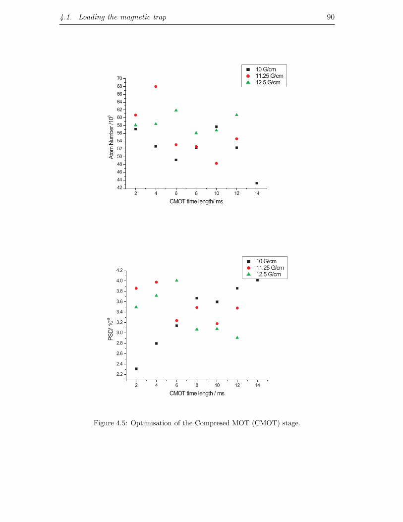
4.1. Loading the magnetic trap 90
2 4 6 8 10 12 14
42
44
46
48
50
52
54
56
58
60
62
64
66
68
70
Ato
mN
um
ber/1
06
CMOT time length/ ms
10 G/cm11.25 G/cm12.5 G/cm
2 4 6 8 10 12 14
2.2
2.4
2.6
2.8
3.0
3.2
3.4
3.6
3.8
4.0
4.2
PS
D/10
-8
CMOT time length / ms
10 G/cm11.25 G/cm12.5 G/cm
Figure 4.5: Optimisation of the Compresed MOT (CMOT) stage.

4.1. Loading the magnetic trap 91
0.0 0.2 0.4 0.6 0.8 1.0 1.2 1.4 1.6
20
22
24
26
28
30
32
34
Reca
ptu
re/%
OP pulse length / ms
Figure 4.6: Percentage of atoms recaptured against pulse length after being held in themagnetic trap for five seconds.
alignment of the laser beams but occasionally the cloud of atoms is hot if any of
the MOT beams has become misaligned. It is generally necessary to realign the
beams once every three months or so to maintain the cold temperature of the cloud
in the magnetic trap.
4.1.4 Optical pumping
The optical pumping of atoms into the F = 1, mF = −1 state takes place immedi-
ately after the optical molasses stage. This is the only low-field seeking mF state
in the F = 1 level and trapping the atoms in this state minimises the problem of
inelastic collisions of atoms due to spin exchange compared to the F = 2 hyperfine
state.
The optical pumping is carried out by exposing the atoms to an optical pumping
beam which is resonant with the 5S 1
2
F = 2 −→ 5P 3
2
F ′ = 2 transition. This beam
needs to be σ− polarised to populate the F = 1, mF = −1 level and therefore
requires a quantisation axis. This field is provided by one of the shim coil pairs
turned on to have 2 Amperes of current running through it during the OP pulse.

4.2. Magnetic trapping 92
This field value was adjusted experimentally to optimise the recapture percentage.
This means noting the fluorescence in the MOT, loading the magnetic trap and
holding the atoms in the magnetic trap for five seconds, and then recapturing
the atoms into the MOT in order to obtain the fluorescence measurement. The
one last task for this stage is to determine the length of this pulse. The optical
pumping beam has a power of 1.5 mW and since this beam comes out the same
fibre as the probing beam, it will have the same 1/e half-width radius as the probe
beam. Figure 4.6 shows the pulse length required to obtain maximum recapture
percentage. We fixed the pulse length to 0.9 ms. Another way to ensure that
the atoms are all in the F = 1, mF = −1 state is to check that when the atoms
are imaged during the absorption imaging stage without being exposed to the
repumper beam, one sees nothing at all. To check for optical pumping efficiency,
we measure recapture rate of atoms immediately after magnetic trap loading. We
typically have 65% conversion into the F = 1, mF = −1 state and a shot-to-shot
noise of about 5% or even less.
4.2 Magnetic trapping
To accurately determine properties of the cloud such as temperature which is
related to the phase space density, it is important to know the trapping frequencies
of our magnetic trap. As mentioned in earlier chapters, at magnetic trap loading,
the current through the coils is 200 Amperes through the overall path and 150
Amperes through the bypass path which leaves 50 Amperes through the bias coils.
4.2.1 Measurement of trapping frequencies
We calculated the magnetic fields and the trapping frequencies numerically when
designing the trap. However, the imprecision in making the coils corresponds to
about 10% uncertainty which makes it impossible to determine the trap frequen-
cies extremely accurately. The most precise way of determining the oscillation
frequency of atoms in the magnetic trap is by using the cloud of atoms. The trap
frequencies are essentially the sloshing frequencies as mentioned previously. We in-
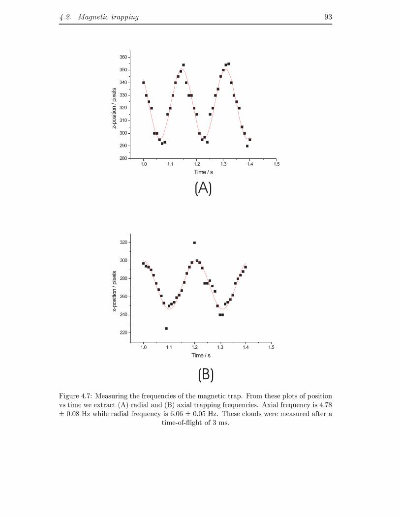
4.2. Magnetic trapping 93
1.0 1.1 1.2 1.3 1.4 1.5
220
240
260
280
300
320
x-posi
tion
/pix
els
Time / s
(A)
(B)
Figure 4.7: Measuring the frequencies of the magnetic trap. From these plots of positionvs time we extract (A) radial and (B) axial trapping frequencies. Axial frequency is 4.78± 0.08 Hz while radial frequency is 6.06 ± 0.05 Hz. These clouds were measured after a
time-of-flight of 3 ms.
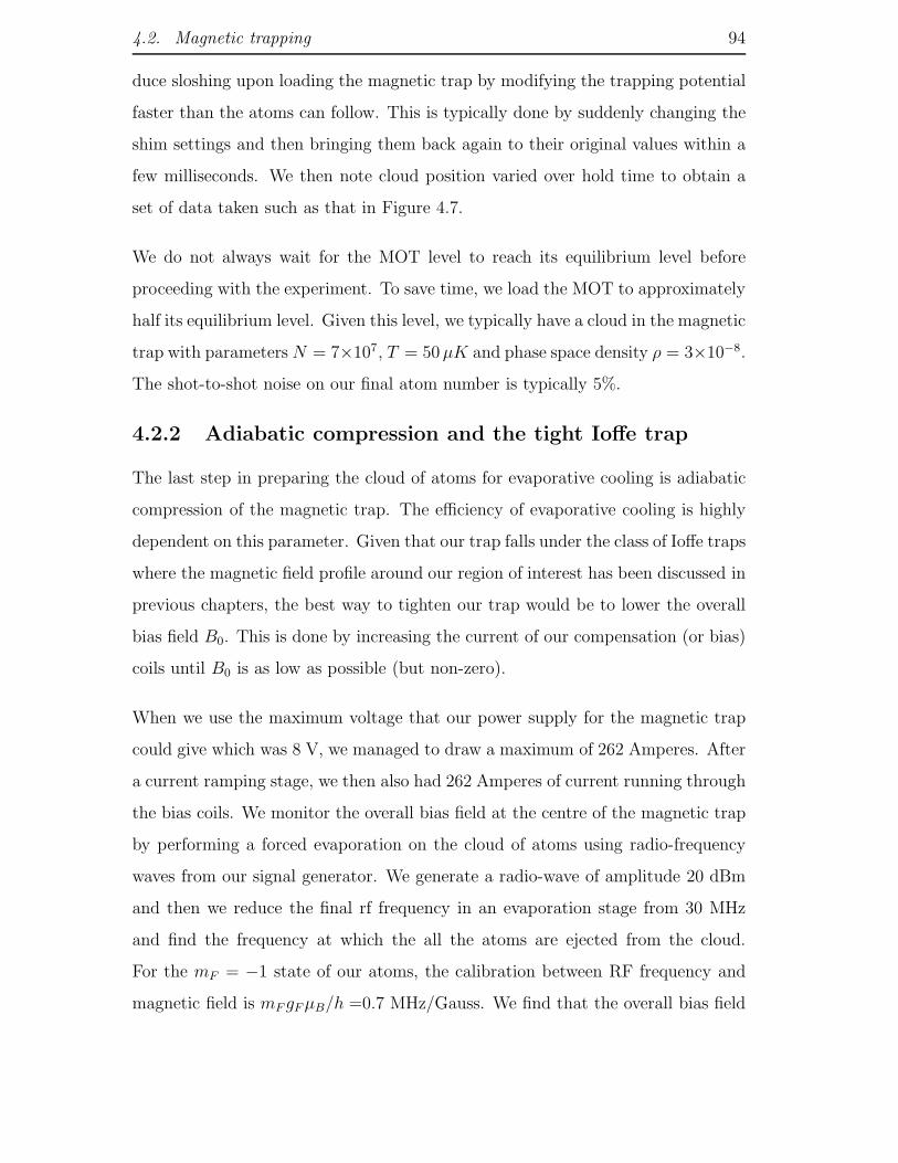
4.2. Magnetic trapping 94
duce sloshing upon loading the magnetic trap by modifying the trapping potential
faster than the atoms can follow. This is typically done by suddenly changing the
shim settings and then bringing them back again to their original values within a
few milliseconds. We then note cloud position varied over hold time to obtain a
set of data taken such as that in Figure 4.7.
We do not always wait for the MOT level to reach its equilibrium level before
proceeding with the experiment. To save time, we load the MOT to approximately
half its equilibrium level. Given this level, we typically have a cloud in the magnetic
trap with parametersN = 7×10⁷, T = 50µK and phase space density ρ = 3×10⁻⁸.
The shot-to-shot noise on our final atom number is typically 5%.
4.2.2 Adiabatic compression and the tight Ioffe trap
The last step in preparing the cloud of atoms for evaporative cooling is adiabatic
compression of the magnetic trap. The efficiency of evaporative cooling is highly
dependent on this parameter. Given that our trap falls under the class of Ioffe traps
where the magnetic field profile around our region of interest has been discussed in
previous chapters, the best way to tighten our trap would be to lower the overall
bias field B0. This is done by increasing the current of our compensation (or bias)
coils until B0 is as low as possible (but non-zero).
When we use the maximum voltage that our power supply for the magnetic trap
could give which was 8 V, we managed to draw a maximum of 262 Amperes. After
a current ramping stage, we then also had 262 Amperes of current running through
the bias coils. We monitor the overall bias field at the centre of the magnetic trap
by performing a forced evaporation on the cloud of atoms using radio-frequency
waves from our signal generator. We generate a radio-wave of amplitude 20 dBm
and then we reduce the final rf frequency in an evaporation stage from 30 MHz
and find the frequency at which the all the atoms are ejected from the cloud.
For the mF = −1 state of our atoms, the calibration between RF frequency and
magnetic field is mF gFµB/h =0.7 MHz/Gauss. We find that the overall bias field
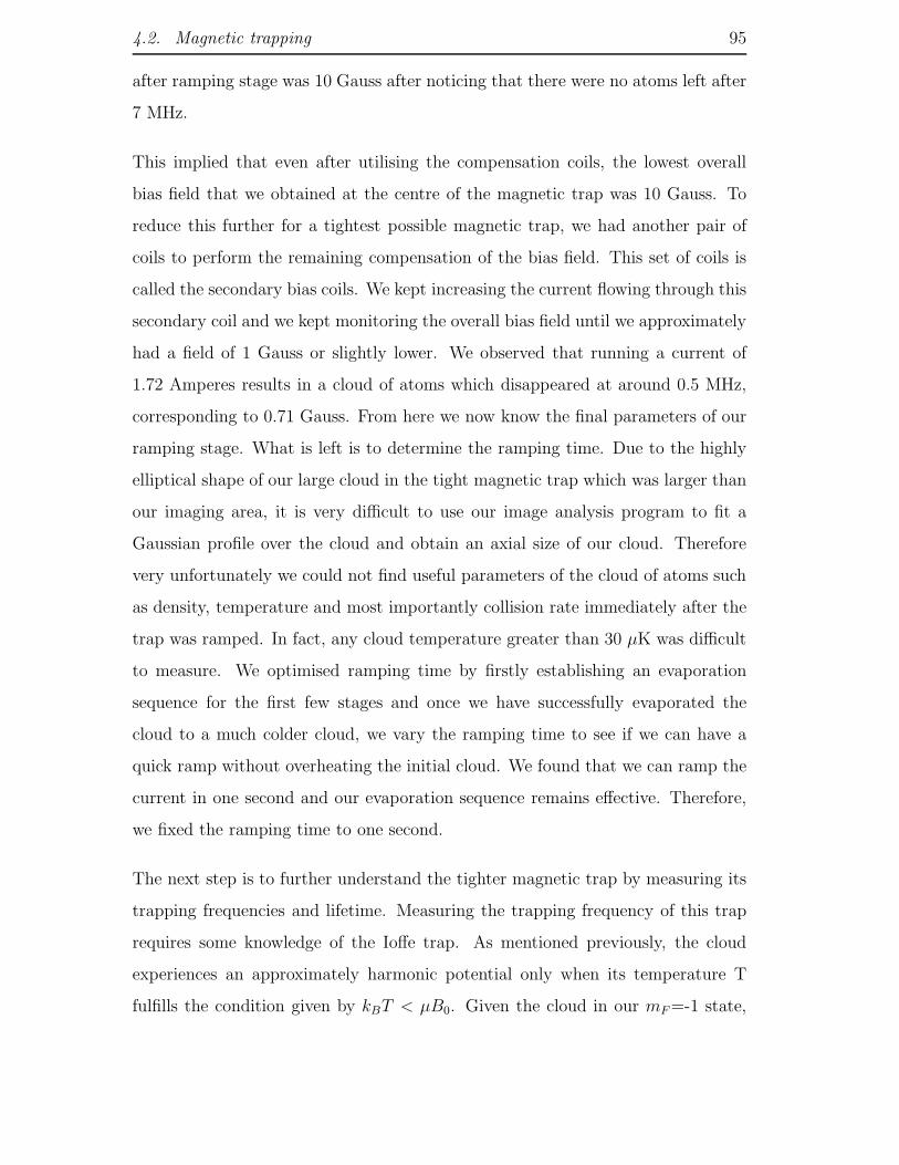
4.2. Magnetic trapping 95
after ramping stage was 10 Gauss after noticing that there were no atoms left after
7 MHz.
This implied that even after utilising the compensation coils, the lowest overall
bias field that we obtained at the centre of the magnetic trap was 10 Gauss. To
reduce this further for a tightest possible magnetic trap, we had another pair of
coils to perform the remaining compensation of the bias field. This set of coils is
called the secondary bias coils. We kept increasing the current flowing through this
secondary coil and we kept monitoring the overall bias field until we approximately
had a field of 1 Gauss or slightly lower. We observed that running a current of
1.72 Amperes results in a cloud of atoms which disappeared at around 0.5 MHz,
corresponding to 0.71 Gauss. From here we now know the final parameters of our
ramping stage. What is left is to determine the ramping time. Due to the highly
elliptical shape of our large cloud in the tight magnetic trap which was larger than
our imaging area, it is very difficult to use our image analysis program to fit a
Gaussian profile over the cloud and obtain an axial size of our cloud. Therefore
very unfortunately we could not find useful parameters of the cloud of atoms such
as density, temperature and most importantly collision rate immediately after the
trap was ramped. In fact, any cloud temperature greater than 30 µK was difficult
to measure. We optimised ramping time by firstly establishing an evaporation
sequence for the first few stages and once we have successfully evaporated the
cloud to a much colder cloud, we vary the ramping time to see if we can have a
quick ramp without overheating the initial cloud. We found that we can ramp the
current in one second and our evaporation sequence remains effective. Therefore,
we fixed the ramping time to one second.
The next step is to further understand the tighter magnetic trap by measuring its
trapping frequencies and lifetime. Measuring the trapping frequency of this trap
requires some knowledge of the Ioffe trap. As mentioned previously, the cloud
experiences an approximately harmonic potential only when its temperature T
fulfills the condition given by kBT < µB0. Given the cloud in our mF =-1 state,

4.3. Evaporative cooling 96
this corresponds to about 33 µK/Gauss. Since our overall bias field was calculated
to be 0.71 Gauss, this means our cloud needs to be significantly lower than 23 µK
before it is in the harmonic region. This therefore means that we have to initially
establish a good evaporation routine which will take our cloud to temperatures
lower than 23 µK. The routine will be further discussed in the next section.
With an initial evaporation sequence, we managed to reduce the temperature of
the cloud to about 300 nK, which is a sufficiently cold cloud we could use to
measure trapping frequencies. As long as the amplitude of the oscillation is small
enough, we can assure ourselves that the cloud remains in a harmonic region of
the magnetic trap. Figure 4.8 shows the measurements leading to the extraction
of the trapping frequencies.
We then measured the lifetime of our cloud in the tight trap. This is a useful
quantity to take note of because it gives us an idea of how much time we have
to complete our evaporation sequence before our atom number fades significantly.
Since at this point our cloud density is not great, our dominant loss mechanisms
would be background collisions with other Rubidium atoms and the cloud being in
an imperfect vacuum. The cloud lifetime was measured by measuring the recapture
rate for various hold times as shown in Figure 4.9.
4.3 Evaporative cooling
4.3.1 Evaporation stages
This section describes the final stage of the experimental sequence to BEC: evapo-
rative cooling. Given that our signal generator (Stanford Research Systems DS345)
could give a maximum frequency of 30 MHz, the first step was to check if there are
atoms in the region of the magnetic trap where the resonance has that frequency.
As it turned out, there was no convincing evidence that there were atoms so far
from the centre of the magnetic trap.
We remove or evaporate the higher energy atoms based on the assumption that

4.3. Evaporative cooling 97
0.0 0.1 0.2 0.3 0.4 0.5 0.6
230
235
240
245
250
255
Clo
ud
posi
tion(x
)/pix
els
Hold time / ms
0.000 0.005 0.010 0.015 0.020
180
190
200
210
220
230
240
Clo
ud
posi
tion
(z)/pix
els
Hold time / ms
(A)
(B)
Figure 4.8: Measuring the oscillation frequencies of atoms in the tight magnetic trap.From these plots we extract (A) axial and (B) radial trapping frequencies. Axial fre-
quency is 5.73 ± 0.03 Hz while radial frequency is 178.6 ± 1.9 Hz.
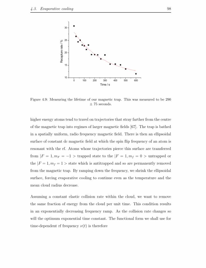
4.3. Evaporative cooling 98
0 100 200 300 400 500 600
10
15
20
25
30
Reca
ptu
rera
te/%
Time / s
Figure 4.9: Measuring the lifetime of our magnetic trap. This was measured to be 290± 75 seconds.
higher energy atoms tend to travel on trajectories that stray farther from the centre
of the magnetic trap into regimes of larger magnetic fields [67]. The trap is bathed
in a spatially uniform, radio frequency magnetic field. There is then an ellipsoidal
surface of constant dc magnetic field at which the spin flip frequency of an atom is
resonant with the rf. Atoms whose trajectories pierce this surface are transferred
from |F = 1, mF = −1 > trapped state to the |F = 1, mf = 0 > untrapped or
the |F = 1, mf = 1 > state which is antitrapped and so are permanently removed
from the magnetic trap. By ramping down the frequency, we shrink the ellipsoidal
surface, forcing evaporative cooling to continue even as the temperature and the
mean cloud radius decrease.
Assuming a constant elastic collision rate within the cloud, we want to remove
the same fraction of energy from the cloud per unit time. This condition results
in an exponentially decreasing frequency ramp. As the collision rate changes so
will the optimum exponential time constant. The functional form we shall use for
time-dependent rf frequency ν(t) is therefore
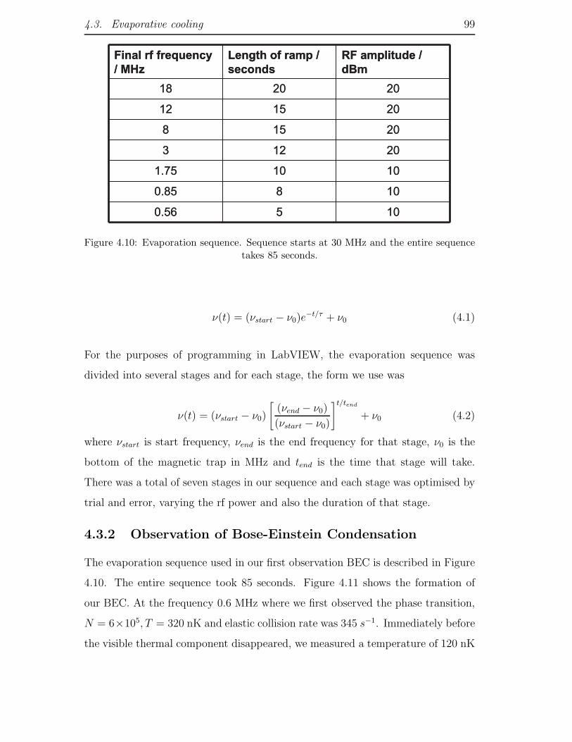
4.3. Evaporative cooling 99
1050.56
1080.85
10101.75
20123
20158
201512
202018
RF amplitude /
dBm
Length of ramp /
seconds
Final rf frequency
/ MHz
1050.56
1080.85
10101.75
20123
20158
201512
202018
RF amplitude /
dBm
Length of ramp /
seconds
Final rf frequency
/ MHz
Figure 4.10: Evaporation sequence. Sequence starts at 30 MHz and the entire sequencetakes 85 seconds.
ν(t) = (νstart − ν0)e−t/τ + ν0 (4.1)
For the purposes of programming in LabVIEW, the evaporation sequence was
divided into several stages and for each stage, the form we use was
ν(t) = (νstart − ν0)
[
(νend − ν0)
(νstart − ν0)
]t/tend
+ ν0 (4.2)
where νstart is start frequency, νend is the end frequency for that stage, ν0 is the
bottom of the magnetic trap in MHz and tend is the time that stage will take.
There was a total of seven stages in our sequence and each stage was optimised by
trial and error, varying the rf power and also the duration of that stage.
4.3.2 Observation of Bose-Einstein Condensation
The evaporation sequence used in our first observation BEC is described in Figure
4.10. The entire sequence took 85 seconds. Figure 4.11 shows the formation of
our BEC. At the frequency 0.6 MHz where we first observed the phase transition,
N = 6×10⁵, T = 320 nK and elastic collision rate was 345 s−1. Immediately before
the visible thermal component disappeared, we measured a temperature of 120 nK
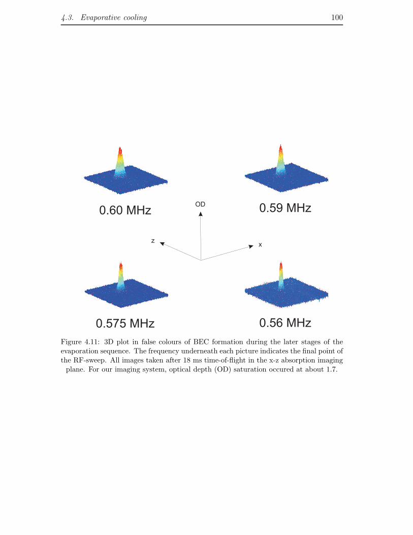
4.3. Evaporative cooling 100
0.60 MHz 0.59 MHz
0.575 MHz 0.56 MHz
xz
OD
Figure 4.11: 3D plot in false colours of BEC formation during the later stages of theevaporation sequence. The frequency underneath each picture indicates the final point ofthe RF-sweep. All images taken after 18 ms time-of-flight in the x-z absorption imaging
plane. For our imaging system, optical depth (OD) saturation occured at about 1.7.
4.3. Evaporative cooling 101
which was done by fitting a Gaussian profile onto the thermal wing of the cloud.
When all visible thermal component have disappeared, we had N = 1.5× 10⁵ in a
pure BEC.
The formation of BEC provided the foundation for the next step which was dipole
trapping of the atoms and potentially manipulation as well.
Chapter 5
Dipole trapping and manipulationof ultra-cold atoms
In this chapter, we describe the procedures used to trap cold atoms in our dipole
trap and to optimise the fluorescence imaging system. Finally, we describe some
experiments that we have done with the atoms in the dipole trap.
5.1 Characterisation of the fluorescence imaging
system
5.1.1 Initial dipole trapping
Throughout this chapter, we shall frequently refer to optical components as labeled
in Figure 5.1. The dipole trapping beam is reflected via mirrors M1, M2 and
dichroic mirror DM1. The dichroic mirror was designed to highly reflect 830 nm
light and highly transmit 780 nm light. At a wavelength of 780 nm, the dichroic
mirror reflects 92% of horizontally-polarised light and 89% of vertically-polarised
light. Whereas at 830 nm, this mirror transmits 81% of horizontally-polarised light
and 92% of vertically-polarised light.
The fluorescence light emitted by the atoms is transmitted through the dichroic
mirror and reflected via mirrors FM1, FM2, FM3 and FM4 before finally being
focused on our CCD camera. We monitor the position on which the focused dipole
102
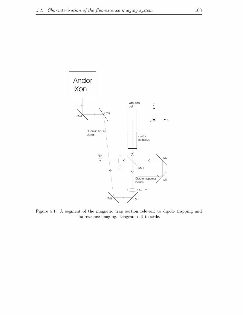
5.1. Characterisation of the fluorescence imaging system 103
Vacuum
cell
4-lens
objective
PSP
M1
M2
DM1
Dipole trapping
beam
f=1 m
FM1FM2
L1
Andor
iXon
FM3FM4
Fluorescence
signal
y
Z
x
Figure 5.1: A segment of the magnetic trap section relevant to dipole trapping andfluorescence imaging. Diagram not to scale.
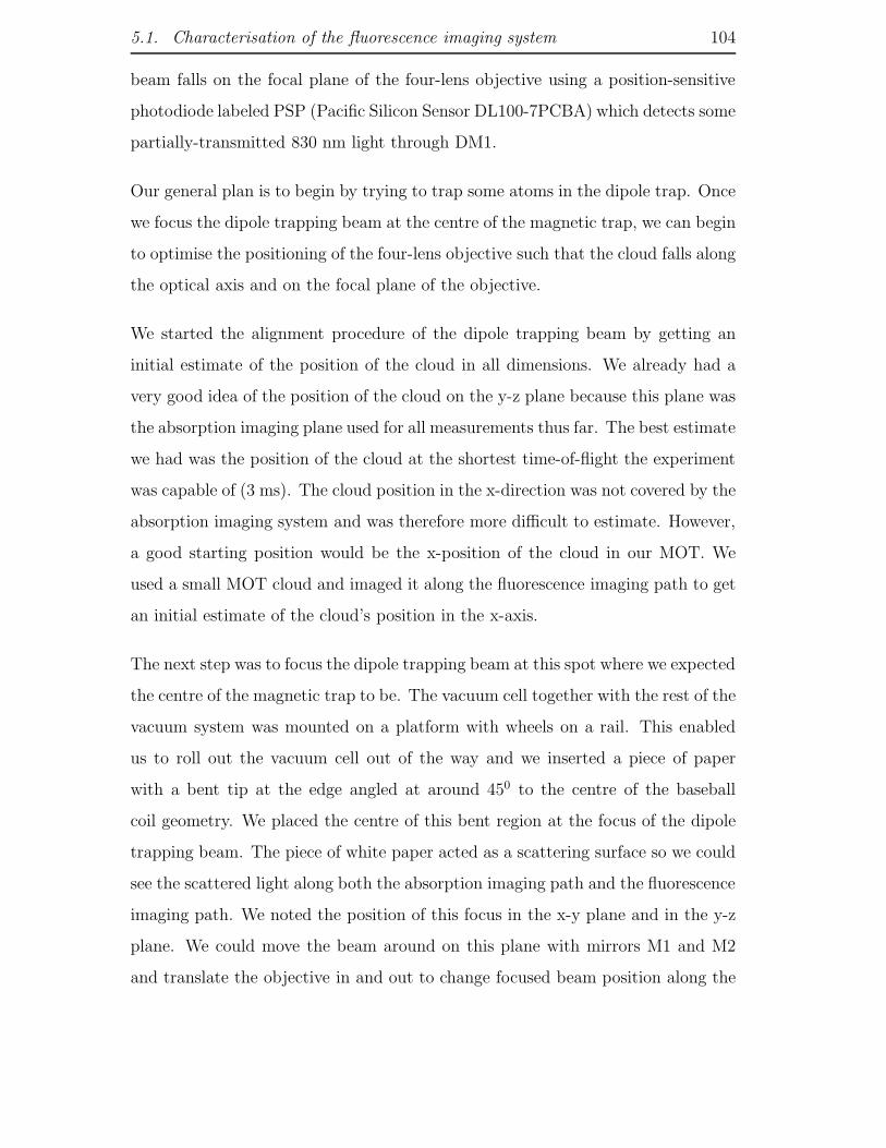
5.1. Characterisation of the fluorescence imaging system 104
beam falls on the focal plane of the four-lens objective using a position-sensitive
photodiode labeled PSP (Pacific Silicon Sensor DL100-7PCBA) which detects some
partially-transmitted 830 nm light through DM1.
Our general plan is to begin by trying to trap some atoms in the dipole trap. Once
we focus the dipole trapping beam at the centre of the magnetic trap, we can begin
to optimise the positioning of the four-lens objective such that the cloud falls along
the optical axis and on the focal plane of the objective.
We started the alignment procedure of the dipole trapping beam by getting an
initial estimate of the position of the cloud in all dimensions. We already had a
very good idea of the position of the cloud on the y-z plane because this plane was
the absorption imaging plane used for all measurements thus far. The best estimate
we had was the position of the cloud at the shortest time-of-flight the experiment
was capable of (3 ms). The cloud position in the x-direction was not covered by the
absorption imaging system and was therefore more difficult to estimate. However,
a good starting position would be the x-position of the cloud in our MOT. We
used a small MOT cloud and imaged it along the fluorescence imaging path to get
an initial estimate of the cloud’s position in the x-axis.
The next step was to focus the dipole trapping beam at this spot where we expected
the centre of the magnetic trap to be. The vacuum cell together with the rest of the
vacuum system was mounted on a platform with wheels on a rail. This enabled
us to roll out the vacuum cell out of the way and we inserted a piece of paper
with a bent tip at the edge angled at around 450 to the centre of the baseball
coil geometry. We placed the centre of this bent region at the focus of the dipole
trapping beam. The piece of white paper acted as a scattering surface so we could
see the scattered light along both the absorption imaging path and the fluorescence
imaging path. We noted the position of this focus in the x-y plane and in the y-z
plane. We could move the beam around on this plane with mirrors M1 and M2
and translate the objective in and out to change focused beam position along the
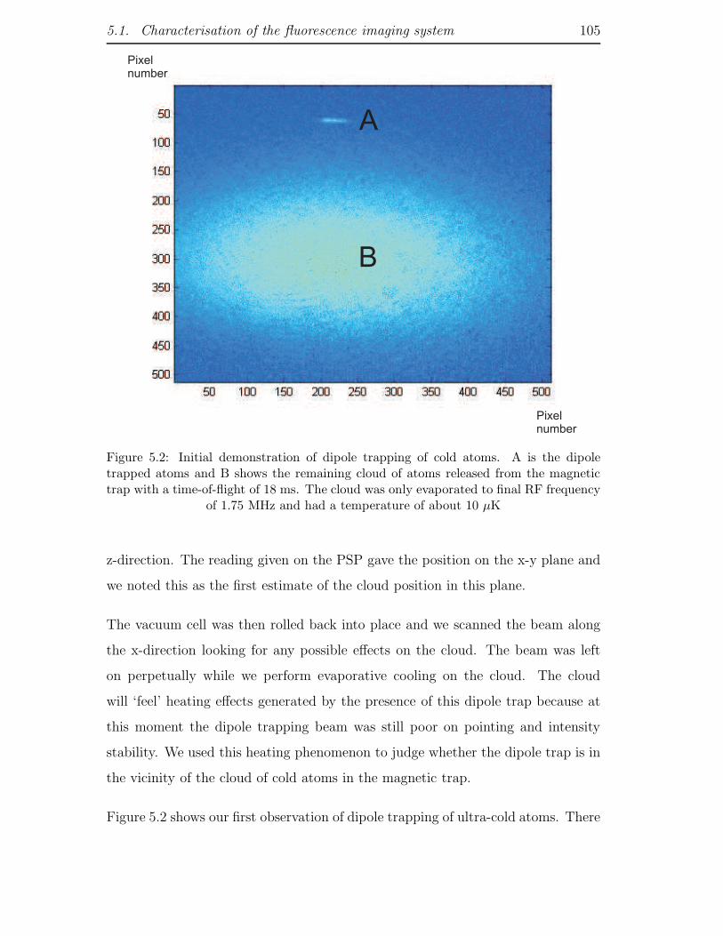
5.1. Characterisation of the fluorescence imaging system 105
A
B
Pixelnumber
Pixelnumber
Figure 5.2: Initial demonstration of dipole trapping of cold atoms. A is the dipoletrapped atoms and B shows the remaining cloud of atoms released from the magnetictrap with a time-of-flight of 18 ms. The cloud was only evaporated to final RF frequency
of 1.75 MHz and had a temperature of about 10 µK
z-direction. The reading given on the PSP gave the position on the x-y plane and
we noted this as the first estimate of the cloud position in this plane.
The vacuum cell was then rolled back into place and we scanned the beam along
the x-direction looking for any possible effects on the cloud. The beam was left
on perpetually while we perform evaporative cooling on the cloud. The cloud
will ‘feel’ heating effects generated by the presence of this dipole trap because at
this moment the dipole trapping beam was still poor on pointing and intensity
stability. We used this heating phenomenon to judge whether the dipole trap is in
the vicinity of the cloud of cold atoms in the magnetic trap.
Figure 5.2 shows our first observation of dipole trapping of ultra-cold atoms. There
5.1. Characterisation of the fluorescence imaging system 106
were 7000 atoms in the trap and the cloud density was 1013 cm−3. The axial half-
width (1/e) of the cloud was 100 µm and radial half-width was 20 µm. One might
notice that the size of this cloud is significantly larger than the size of the dipole
trapping beam that we would expect (about a few µm). Given that the number of
atoms loaded into the dipole trap was considerably large by dipole trap standards,
illuminating it with our probing beam causes the atoms to absorb and re-emit
while other atoms reabsorb and diffuse out in the process. This situation is similar
to the density-limited regime in a Magneto-Optical Trap (MOT).
Once we were confident the focused beam was very close to the centre of the cloud,
we no longer left the dipole trapping beam on during the experiment but waited
until the end of the evaporation sequence after which the power of the beam focused
on the atoms was ramped from 0 to 20 mW in 1 second. Immediately after this
beam intensity ramp, the cloud of atoms was under the influence of a magnetic
trap and a dipole trap simultaneously. So to separate the dipole trapped atoms
from the magnetically trapped atoms, the magnetic trap was turned off and we
waited for a further 18 ms of time to ensure that the cloud from the magnetic trap
has fallen a significant distance. Afterwards, the cloud is imaged with absorption
imaging while the atoms are still in the dipole trap.
The final step was to align the dipole beam to the centre of the cloud. This was
done by reducing the final RF evaporation frequency gradually to get smaller clouds
and seeing if atoms could still be loaded into the dipole trap. Once dipole trapping
no longer occured, the position of the focused dipole trapping beam was adjusted
using mirror M1 (or M2) for movement in the x or y-direction and translating
the objective in the z-direction for movement in the z-direction to observe dipole
trapping again. This procedure was then repeated until we could still load atoms
from a very small cloud. Then we were confident that our dipole trapping beam
was focused at the centre of the magnetic trap.
5.1. Characterisation of the fluorescence imaging system 107
5.1.2 Positioning the four-lens objective
After focussing the dipole trapping beam onto the centre of the magnetic trap,
the next step was to optimise the positioning of the four-lens objective. Ideally,
the cloud should be at the focal plane and along the optical axis of the four-lens
objective. At the same time, the dipole trapping beam should also be entering the
aperture of the objective along the axis of the objective.
The first step to this procedure was to roll out the vacuum cell again. We then
inserted a USAF 1951 standard pattern R70 test image. The test image was glued
on a stick which was glued on a mirror mount for fine and precise movement. The
entire mirror mount was then fixed on a translation stage with the mount’s move-
ment parallel to the dipole trapping beam axis. The test image was illuminated
from behind by the pyramidal MOT cooling beam and from the front by the dipole
trapping beam. The test slide was manufactured from glass and mirror-coated on
one side and could therefore act as a reflecting surface. In addition, the features
on the test plate were transparent and would therefore transmit the pyramidal
MOT light. The light transmitted through DM1 consisted of the reflected dipole
trapping beam and the pyramidal MOT beam and it was focused onto the CCD
camera using a lens of focal length 1 m. The test image could be translated in
three dimensions to place the finest set of lines on the focused dipole beam. Tem-
porarily, the location of the finest set of lines was the reference position of the
magnetic trap.
The four-lens objective was mounted on a five-axis mount (X, Y, Z, pitch and
yaw) and all five axes could be adjusted to ensure that the finest set of lines could
be resolved. In fact, if we placed a white piece of paper between FM2 and FM3
and used an infra-red viewer to see the fluorescence light falling on the paper, we
could also see the field-of-view of the four-lens objective. We then translated the
objective to place the reference position of the magnetic trap at the centre of this
field-of-view. Further adjustment of the five axes resolved the finest set of lines as
shown in Figure 5.1.
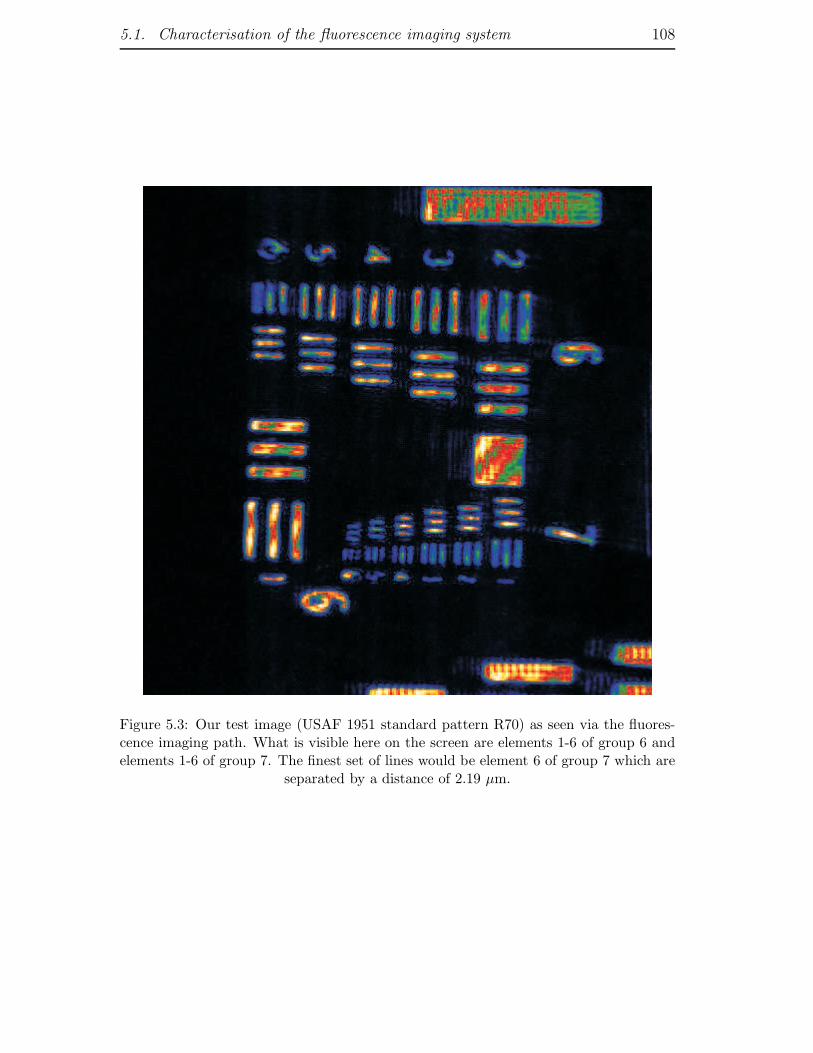
5.1. Characterisation of the fluorescence imaging system 108
Figure 5.3: Our test image (USAF 1951 standard pattern R70) as seen via the fluores-cence imaging path. What is visible here on the screen are elements 1-6 of group 6 andelements 1-6 of group 7. The finest set of lines would be element 6 of group 7 which are
separated by a distance of 2.19 µm.
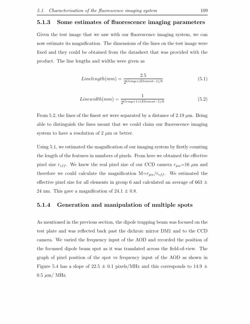
5.1. Characterisation of the fluorescence imaging system 109
5.1.3 Some estimates of fluorescence imaging parameters
Given the test image that we saw with our fluorescence imaging system, we can
now estimate its magnification. The dimensions of the lines on the test image were
fixed and they could be obtained from the datasheet that was provided with the
product. The line lengths and widths were given as
Linelength(mm) =2.5
2Group+(Element−1)/6(5.1)
Linewidth(mm) =1
2Group+1+(Element−1)/6(5.2)
From 5.2, the lines of the finest set were separated by a distance of 2.19 µm. Being
able to distinguish the lines meant that we could claim our fluorescence imaging
system to have a resolution of 2 µm or better.
Using 5.1, we estimated the magnification of our imaging system by firstly counting
the length of the features in numbers of pixels. From here we obtained the effective
pixel size reff . We knew the real pixel size of our CCD camera rpix=16 µm and
therefore we could calculate the magnification M=rpix/reff . We estimated the
effective pixel size for all elements in group 6 and calculated an average of 663 ±24 nm. This gave a magnification of 24.1 ± 0.8.
5.1.4 Generation and manipulation of multiple spots
As mentioned in the previous section, the dipole trapping beam was focused on the
test plate and was reflected back past the dichroic mirror DM1 and to the CCD
camera. We varied the frequency input of the AOD and recorded the position of
the focussed dipole beam spot as it was translated across the field-of-view. The
graph of pixel position of the spot vs frequency input of the AOD as shown in
Figure 5.4 has a slope of 22.5 ± 0.1 pixels/MHz and this corresponds to 14.9 ±0.5 µm/ MHz.
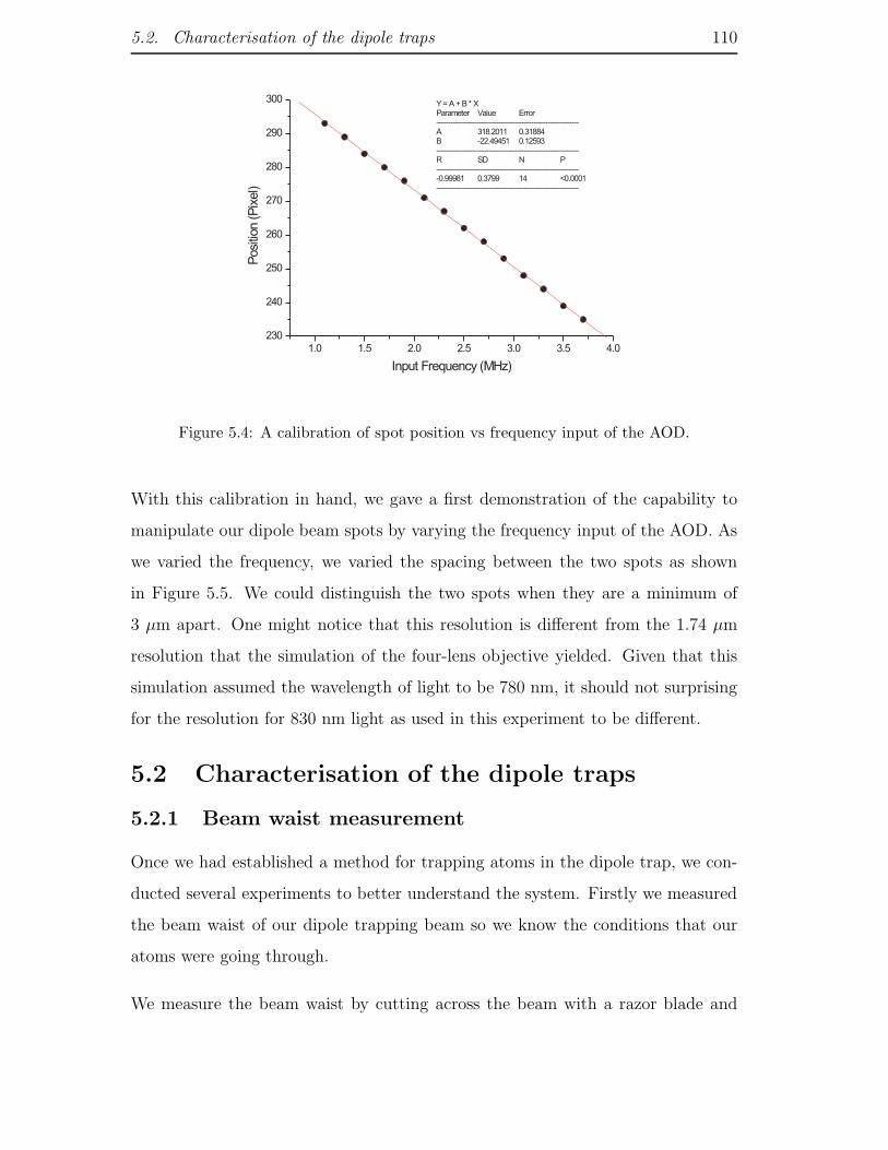
5.2. Characterisation of the dipole traps 110
1.0 1.5 2.0 2.5 3.0 3.5 4.0
230
240
250
260
270
280
290
300Y= A + B * XParameter Value Error------------------------------------------------------------A 318.2011 0.31884B -22.49451 0.12593------------------------------------------------------------R SD N P-------------------------------------------------------------0.99981 0.3799 14 <0.0001------------------------------------------------------------
Posi
tion
(Pix
el)
Input Frequency (MHz)
Figure 5.4: A calibration of spot position vs frequency input of the AOD.
With this calibration in hand, we gave a first demonstration of the capability to
manipulate our dipole beam spots by varying the frequency input of the AOD. As
we varied the frequency, we varied the spacing between the two spots as shown
in Figure 5.5. We could distinguish the two spots when they are a minimum of
3 µm apart. One might notice that this resolution is different from the 1.74 µm
resolution that the simulation of the four-lens objective yielded. Given that this
simulation assumed the wavelength of light to be 780 nm, it should not surprising
for the resolution for 830 nm light as used in this experiment to be different.
5.2 Characterisation of the dipole traps
5.2.1 Beam waist measurement
Once we had established a method for trapping atoms in the dipole trap, we con-
ducted several experiments to better understand the system. Firstly we measured
the beam waist of our dipole trapping beam so we know the conditions that our
atoms were going through.
We measure the beam waist by cutting across the beam with a razor blade and
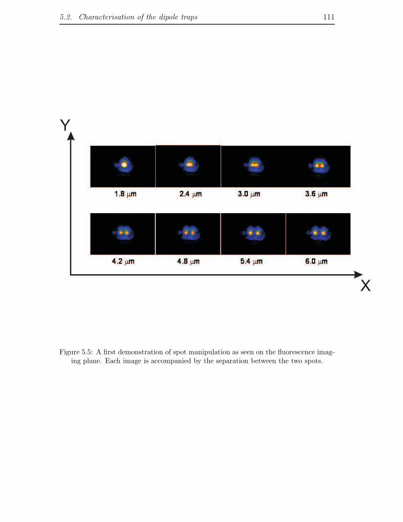
5.2. Characterisation of the dipole traps 111
X
Y
Figure 5.5: A first demonstration of spot manipulation as seen on the fluorescence imag-ing plane. Each image is accompanied by the separation between the two spots.

5.2. Characterisation of the dipole traps 112
2.00 2.02 2.04 2.06 2.08 2.10
-100
0
100
200
300
400
500
600
700
800
Inte
nsi
ty/arb
itrary
Position / mm
(A)
(B)
13.4 13.6 13.8 14.0 14.2 14.4
0
10
20
30
40
50
60
1/e
beam
wais
t/?m
Position / mm
Figure 5.6: Beam waist measurements of our dipole trapping beam. (A) shows the beamwaists attained w.r.t position of the blade. (B) shows a reconstruction of our dipole
trapping beam.
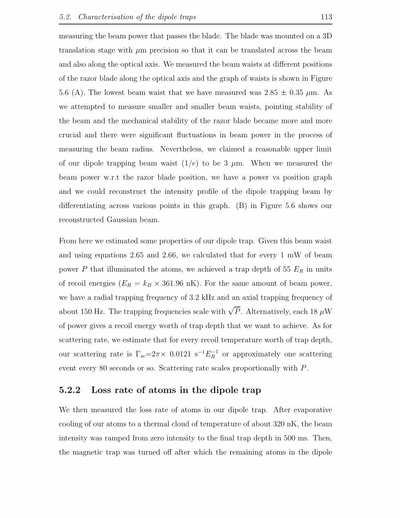
5.2. Characterisation of the dipole traps 113
measuring the beam power that passes the blade. The blade was mounted on a 3D
translation stage with µm precision so that it can be translated across the beam
and also along the optical axis. We measured the beam waists at different positions
of the razor blade along the optical axis and the graph of waists is shown in Figure
5.6 (A). The lowest beam waist that we have measured was 2.85 ± 0.35 µm. As
we attempted to measure smaller and smaller beam waists, pointing stability of
the beam and the mechanical stability of the razor blade became more and more
crucial and there were significant fluctuations in beam power in the process of
measuring the beam radius. Nevertheless, we claimed a reasonable upper limit
of our dipole trapping beam waist (1/e) to be 3 µm. When we measured the
beam power w.r.t the razor blade position, we have a power vs position graph
and we could reconstruct the intensity profile of the dipole trapping beam by
differentiating across various points in this graph. (B) in Figure 5.6 shows our
reconstructed Gaussian beam.
From here we estimated some properties of our dipole trap. Given this beam waist
and using equations 2.65 and 2.66, we calculated that for every 1 mW of beam
power P that illuminated the atoms, we achieved a trap depth of 55 ER in units
of recoil energies (ER = kB × 361.96 nK). For the same amount of beam power,
we have a radial trapping frequency of 3.2 kHz and an axial trapping frequency of
about 150 Hz. The trapping frequencies scale with√P . Alternatively, each 18 µW
of power gives a recoil energy worth of trap depth that we want to achieve. As for
scattering rate, we estimate that for every recoil temperature worth of trap depth,
our scattering rate is Γsc=2π× 0.0121 s−1E−1R or approximately one scattering
event every 80 seconds or so. Scattering rate scales proportionally with P .
5.2.2 Loss rate of atoms in the dipole trap
We then measured the loss rate of atoms in our dipole trap. After evaporative
cooling of our atoms to a thermal cloud of temperature of about 320 nK, the beam
intensity was ramped from zero intensity to the final trap depth in 500 ms. Then,
the magnetic trap was turned off after which the remaining atoms in the dipole

5.2. Characterisation of the dipole traps 114
0 100 200 300 400 500
0
5000
10000
15000
20000
25000
No.ofato
ms
Hold time / ms
0.42 mW = 23 ER
? = (73 +/- 11) ms
0 100 200 300 400 500
500
1000
1500
2000
2500
3000
No.ofato
ms
Hold time / ms
2.60 mW = 140 ER
? = (83 +/- 17) ms
0 100 200 300 400 500
1000
2000
3000
4000
5000
No.ofato
ms
Hold time / ms
6.2 mW = 330 ER
? = (79 +/- 10) ms
Figure 5.7: Measurement of the rate of loss of atoms in our dipole trap. Loss rates areshown as τ−1.
5.2. Characterisation of the dipole traps 115
trap were given a certain hold time before images were taken to measure how many
atoms were left in the dipole trap. We varied the hold time for a certain trap depth
to measure the loss rate and we measured this for three different trap depths. The
graphs are shown in Figure 5.7.
Given that from results above the loss rate of the atoms in the dipole trap were
independent of our trap depth, these seem to suggest that our loss rate does not
correspond to the true lifetime of the atoms in our dipole trap. A possible reason
is there are atoms with energies very close to the value required to escape the trap
and this loss rate implies those atoms escaping first before stabilising to some other
equilibrium value of atom number.
This loss rate could also be due to a combination of processes of background
collisions, 2-body and 3-body inelastic collisions. Taking into account these loss
mechanisms, the loss rate of atoms is given by
dN
dt= −N
τb−K2 < n > N −K3 < n2 > N (5.3)
where τb is the loss rate for background collisions and K2 and K3 are loss rates
for 2-body and 3-body inelastic collisions respectively. In addition, we must also
consider losses from heating due to pointing and intensity stability of the dipole
trapping beam. At this moment, our loss rate could be a mixture of the above
processes and so does not reflect the true lifetime of our atoms in the dipole trap.
Understanding this would require further investigation in the future.
5.2.3 Probing sequence
To resolve these narrowly separated dipole traps, we need to be able to observe the
dipole trapped atoms via the fluorescence imaging system. Initially, to maximise
observed signal, we changed the settings of our Andor iXon CCD camera to greatly
increase its sensitivity. We increased the pre-amplifier gain to the maximum possi-
ble value of 5.1 and also increased the Electron Multiplying Charged-Couple Device
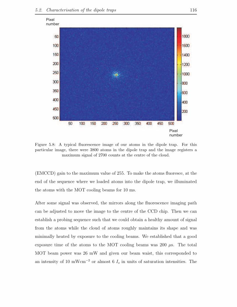
5.2. Characterisation of the dipole traps 116
Pixelnumber
Pixelnumber
Figure 5.8: A typical fluorescence image of our atoms in the dipole trap. For thisparticular image, there were 3800 atoms in the dipole trap and the image registers a
maximum signal of 2700 counts at the centre of the cloud.
(EMCCD) gain to the maximum value of 255. To make the atoms fluoresce, at the
end of the sequence where we loaded atoms into the dipole trap, we illuminated
the atoms with the MOT cooling beams for 10 ms.
After some signal was observed, the mirrors along the fluorescence imaging path
can be adjusted to move the image to the centre of the CCD chip. Then we can
establish a probing sequence such that we could obtain a healthy amount of signal
from the atoms while the cloud of atoms roughly maintains its shape and was
minimally heated by exposure to the cooling beams. We established that a good
exposure time of the atoms to the MOT cooling beams was 200 µs. The total
MOT beam power was 26 mW and given our beam waist, this corresponded to
an intensity of 10 mWcm−2 or almost 6 Is in units of saturation intensities. The
5.2. Characterisation of the dipole traps 117
laser detuning of our MOT beams was δ= -9 MHz. Figure 5.8 shows a typical
image of our atoms in the dipole trap. The typical cloud radial width (1/e) that
we obtained was 20 µm.
With this probing sequence, we calculated how the number of counts we obtained
via fluorescence imaging would correspond to the true number of atoms by cali-
bration against absorption imaging. Assuming that a cloud of atoms in our dipole
trap could be attained reproducibly, there should be an equal number of atoms
regardless of our imaging method.
For an arbitrary dipole trapping sequence, when we ran the experiment ten times
using absorption imaging, we had (4.11 ± 0.60) × 103 atoms. We then switched
immediately to fluorescence imaging; running the same experiment ten times, we
registered (1.27 ± 0.11) × 106 counts on the CCD camera. Therefore, for a number
of atoms Natoms and number of counts Ncounts that we have just measured, calibra-
tion was obtained by including an imaging factor α such that Natoms = αNcounts.
This imaging factor was then included permanently in the image processing pro-
gram to calculate our number of atoms in the dipole trap. Given that the signal-
to-noise ratio is good only for low atom numbers for fluorescence imaging (see
Appendix D), this calibration was only useful for measurement of low atom num-
bers. Now that we have the above expression, we measured α = (3.24±0.55)×10−3
or 300 counts/atom with a 17% error. Conveniently, this imaging factor took into
consideration absolutely all factors such as pre-amplifier gain, EMCCD gain, solid
angle presented by the four-lens objective, MOT beam intensity, exposure time
and signal losses via all optical components.
5.2.4 Low atom number detection
With this calibration, we tried to detect as low an atom number as possible so
as to gauge the capability of our imaging system. When an image is taken, it is
essentially a 512 × 512 matrix where elements record the number of counts detected
on each pixel. We conclude that the imaging system is capable of detecting a

5.2. Characterisation of the dipole traps 118
50 100 150 200 250 300 350 400 450-1
0
1
2
3
4
5
6x 10
4
50 100 150 200 250 300 350 400 450-1
0
1
2
3
4
5
6x 10
4
50 100 150 200 250 300 350 400 450-1
0
1
2
3
4
5
6x 10
4
50 100 150 200 250 300 350 400 450-1
0
1
2
3
4
5
6x 10
4
6600 atoms
1300 atoms
500 atoms
No atoms
No. of counts
No. of counts
No. of counts
No. of counts
Pixel number
Pixel number
Pixel number
Pixel number
Figure 5.9: Low atom number detection by the fluorescence imaging system. All atomnumbers shown have a 17 % error.

5.2. Characterisation of the dipole traps 119
certain number of atoms by summing this matrix in one direction and if we see
this profile of integrated counts by eye, one should clearly see the presence of signal
emitted from the atoms. Graphs of integrated counts for different atom numbers
are shown in Figure 5.9. These graphs were compared with a typical graph where
no atoms were observed and it was clear that as it stood, our fluorescence imaging
system was capable of detecting about 500 atoms at the lowest. In the near future,
we hope to improve this system to be able to detect single atoms.
5.2.5 Generation and manipulation of multiple dipole traps
An integral part of this experiment was the ability to manipulate the dipole traps.
Our Arbitrary Waveform Generator (AWG) provided a carrier frequency ν0 of 50
MHz and this carrier signal was mixed with an additional signal δν generated by
a 20 MHZ signal generator. As a result, we have two different signals of frequency
ν0 ± δν and this results in the generation of multiple dipole trapping beams which
focussed via the four-lens objective to form multiple dipole traps. By varying δν,
we could vary the separation between the two spots. A demonstration of this
is shown in Figure 5.10 where we loaded the atoms from a partially-evaporated
thermal cloud into multiple dipole traps. With this demonstration, we have made
significant significant progress towards achieving addressability of individual lattice
sites.
This experiment could be expanded to try varying the array configuration of the
multiple dipole traps. As shown in the setup in Figure 3.16, our AOD could deflect
light in the X and the Y axes because the carrier frequency that we started with
could also be mixed in both axes to generate multiple deflection of light in the X
and Y axis. We have successfully loaded atoms into a single spot, 1 × 2 array, 1
× 3 array and 2 × 2 array of optical dipole traps. Loading of atoms into these
traps was demonstrated and images are shown in Figure 5.11. This was again one
very big step forward in achieving a 2-dimensional array optical lattice where the
lattice sites were completely manipulable.
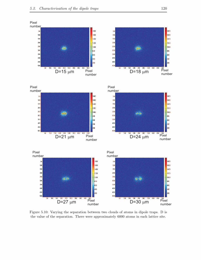
5.2. Characterisation of the dipole traps 120
D=15 mm D=18 mm
D=21 mm D=24 mm
D=27 mm D=30 mm
Pixelnumber
Pixelnumber
Pixelnumber
Pixelnumber
Pixelnumber
Pixelnumber
Pixelnumber
Pixelnumber
Pixelnumber
Pixelnumber
Pixelnumber
Figure 5.10: Varying the separation between two clouds of atoms in dipole traps. D isthe value of the separation. There were approximately 6000 atoms in each lattice site.
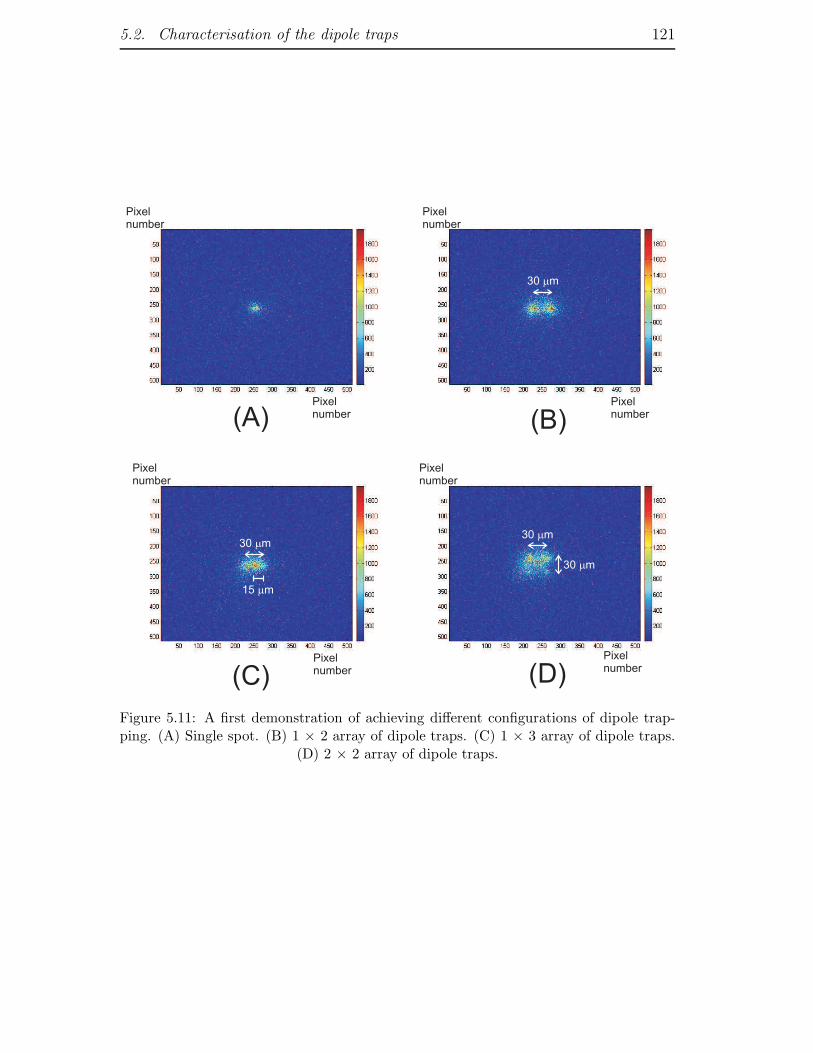
5.2. Characterisation of the dipole traps 121
(A) (B)
(C) (D)
30 mm
30 mm
30 mm
30 mm
15 mm
Pixelnumber
Pixelnumber
Pixelnumber
Pixelnumber
Pixelnumber
Pixelnumber
Pixelnumber
Pixelnumber
Figure 5.11: A first demonstration of achieving different configurations of dipole trap-ping. (A) Single spot. (B) 1 × 2 array of dipole traps. (C) 1 × 3 array of dipole traps.
(D) 2 × 2 array of dipole traps.

5.2. Characterisation of the dipole traps 122
Finally, we try to understand what the various limitations of this method of dipole
trap splitting might be. Firstly, given that our AOD has a total bandwidth of 25
MHz and given our calibration, we estimate that a single trap can be moved by
a total distance of more than 370 µm from one side to the other. Now that we
also know our resolution of distinguishing multiple spots to be 3 µm, this implies
that we can have a maximum of 123 lattice sites per axis. With our current
method of operation, we know too that lattice sites in our setup can only be
moved in rows and/or columns. Moreover, our setup is only capable of generating
a 2-dimensional optical lattice. While generating a 3-dimensional lattice is not
impossible using our setup, at this moment there is enough interesting physics to
study with just a 2-D lattice. As with all other traps, our dipole trap needs to
fulfill certain stability requirements to avoid heating of the cloud or decoherence of
the condensate. A formal treatment of these requirements with respect to pointing
and intensity stabilities can be found in [68].
Nevertheless, this method of operation has its advantages over other methods. For
example, this setup will have much more precise control of lattice sites compared
to dipole traps created by holographic methods (eg. spatial light modulator).
Our dipole trap manipulation is also not restricted like that in traps generated by
microlens arrays. Our apparatus offers greater flexibility and addressability than
optical lattices where the latice separation is typically of the order of hundreds of
nanometres and our trapping mechanism is not dependent on spin states like that
in atom chips.
Chapter 6
Conclusion and future work
6.1 Achievements so far
While there is still much to do, a lot has already been achieved since the experi-
ment started its construction phase in October 2003. Our first milestone was the
successful building of the experiment which produced BEC. As mentioned, we had
about 10 5 atoms in our pure BEC which was much more than what we will ever
need for our Mott Insulator (MI) experiments.
Our next two milestones were demonstrating that we could load cold atoms into
the dipole trap and seeing those atoms by fluorescence imaging. This process has
been reproducible so far and this is very important. With the magnification that
we currently have, we hope to be able to observe processes such as trap splitting
and displacement. Given our probing sequence, we have also detected low atom
numbers although admittedly, our current probing sequence still has room for
improvement.
Finally, we have demonstrated dipole trap manipulation and also successfully cre-
ated a small 2 × 2 optical lattice. While we aim to be more ambitious with
the optical lattice, this demonstration was a very big step forward and laid the
foundation for the work ahead.
123

6.2. Future work 124
6.2 Future work
Before we begin qubit manipulation experiments, there are several things that need
to be done.
6.2.1 Adiabatic loading of BEC
While we have successfully loaded cold atoms into the dipole trap, there is a need
to determine whether this process is adiabatic. The best way to do this is to check
that a condensate loaded into a dipole trap remains a condensate. This could be
done by loading some atoms into a dipole trap after which the magnetic trap could
be switched off to remove atoms still trapped in the magnetic trap. The dipole
trap could then be split into two separate traps located close to each other and
then be turned off abruptly. The two condensates will fall and expand. If the two
clouds are still condensates after loading into the dipole trap, they will interfere
when they overlap and interference patterns will be observed.
There are two things to consider in order to achieve this. One would be intensity
stability and how the intensity is ramped. As for the former, we have set up
a prototype intensity servo device into our experiment which helped keep our
intensity stable reduce beam power fluctuations when the beam intensity is ramped
from one value to another. As for the latter, the time taken and the functional
form of the ramp can be varied to achieve adiabaticity.
When we have demonstrated that atoms have been adiabatically loaded into the
trap, we can then ensure that the atoms are at the lowest energy state of the dipole
trap. This corresponds to the atoms being in the harmonic region and then we can
also measure the trapping frequencies of the dipole trap given the beam intensity.
Knowing the trapping frequencies will allow us to more accurately calculate the
temperature of our cloud and will give us more information regarding the true
waist of our dipole trapping beam.

6.2. Future work 125
6.2.2 Imaging and single atom detection
Having the atoms in our dipole trap in a condensate form means our cloud of
atoms is in the densest possible state and thus the ideal test object to check if our
imaging system is focussed. We can then measure the magnification of the imaging
system by measuring the apparent acceleration due to gravity of a falling cloud of
atoms released from the dipole trap. This method was also used to measure the
magnification of our absorption imaging system.
Having a focused imaging system results in the highest possible signal concentra-
tion and this greatly improves our capability of detecting very low atom numbers.
While the experiment has shown to be able to detect about 500 atoms, ideally we
would like to detect single atoms. Another thing that can be tried is changing the
probing sequence to maximise signal and minimise noise at the same time.
6.2.3 2D optical lattice and the Mott Insulator state
In this experiment, we have demonstrated several possible configurations of 2D
optical lattice. These are the single dipole trap, the 1 × 2 array, the 1 × 3 array
and the 2 × 2 array. So far, we did this using a setup of a main signal generator to
provide the carrier frequency, an additional signal generator and an RF mixer to
provide the multiple frequency signal input into the AOD. The schematic of this
setup is shown in Figure 3.16. We hope to improve the current setup by using a
custom-built circuit board incorporating ten Direct Digital Synthesis (DDS) chips
with a common 20 MHz clock to potentially provide ten sinusoidal signals with
independent, dynamically variable frequencies. We wish for two of these boards to
be made, one for the X axis and the other for the Y axis. This means that we will
soon be capable of a 10 × 10 array of dipole traps, similar to a 2D optical lattice.
Once this board is set to work reproducibly, the next step is to use the board to
successfully produce the multiple frequency inputs to the AOD to generate multiple
dipole traps with atoms loaded into them. Not only that, it must be demonstrated
that these traps can split adiabatically. Again, the best way to check this is to make
6.2. Future work 126
sure that the condensate that is loaded into these traps remain in condensate form.
When the dipole traps are released and the expanded clouds overlap, interference
patterns should be observed.
Finally, before we can claim to be ready for qubit manipulation and possibly
other experiments, we need to reproduce the Mott Insulator state as it is vital
for quantum information processing that the atom number is distributed evenly
amongst the lattice sites. We hope to do this by repeating the method as mentioned
in [8] where quantum tunneling between lattice sites is suppressed by increasing the
potential barrier between the sites. This is done by increasing the dipole trapping
beam intensity and therefore the trap depth of each lattice site. As tunneling rates
are suppressed, the interference pattern we expect to see when the atoms are in
the superfluid state will start to lose its definition. Alternatively, we can verify the
MI state by direct atom number counting [61] and verifying that the fluctuation
of the measured atom number is lower than the Standard Quantum Limit (SQL).

Appendix A
Rubidium-87 data
Relevant physical properties for Rb-87 atoms are given below. For the cases where
these depend on the specific atomic transition, they are given for the D2 line of
Rb-87.
Quantity Symbol Value
Atomic number Z 37Nuclear spin I 3/2
Mass m 1.443 × 10⁻²⁵ kgWavelength (vacuum) λ 780.241 nm
Wave number (vacuum) k/2π 12816.5 cm−1
Natural linewidth (FWHM) Γ 2π · 6.065 MHzDecay rate 38.11 × 10⁶ s−1
Saturation intensity π-pol Isat 2.503 mW cm−2
(F = 2 → F ′ = 3)Resonant cross section π-pol σ0 1.938 × 10⁻⁹ cm2
Saturation intensity σ-pol Isat 1.67 mW cm−2
(|F = 2, mF = ±2〉 → |F ′ = 3, mF ′ = ±3〉)Resonant cross section σ-pol σ0 2.907 × 10⁻⁹ cm2
Recoil velocity vr = hk/m 5.88 mm s−1
Recoil temperature Tr = mv2r /kB 362 nK
Zeeman shift of 5S1/2 F = 2 1/2 µB ×mF 700 kHz G−1 ×mF
Zeeman shift of 5P3/2 F = 3 2/3 µB ×mF 933 kHz G−1 ×mF
Scattering length at B = 0 a 5.31 nm|F = 1, mF = 1〉
127

Appendix B
Beam waist measurement
The setup for measurement of a beam waist consists of a razor blade mounted on
a translation stage. The blade is translated finely to cut into the beam. The beam
power past the blade is then measured and the beam power vs position profile will
provide us information regarding the size of the beam. This section derives the
functional form used to fit to such a profile.
The first assumption is that the beam in question is of a Gaussian profile which
stretches from +∞ to −∞, is centred at x=0 and has a (1/e) width σ. With the
razor blade partially into the beam at some position x0, the power measured past
the blade would be the integral of the intensity profile from ∞ to x0:
P = I0
∫ ∞
x0
e−x2/σ2
dx
= I0
∫ 0
x0
e−x2/σ2
dx+∫ ∞
0e−x2/σ2
dx
(B.1)
The substitution t2 = x2/σ2 and therefore dx=σdt can be used. The special
integral∫∞−∞ e−t2 dt =
√π should also be substituted to transform equation B.1 to
P = I0σ
∫ 0
x0/σe−t2 dt+
√π
2
128
129
=I0σ
√π
2
1 − 2√π
∫ x0/σ
0e−t2 dt
= A
1 − erf(x0/σ)
(B.2)
and this is the form of the fitting expression used to extract the beam waist (1/e).
Appendix C
Calculating atom number from aMagneto-Optical trap
The number of atoms in a MOT can be estimated using fluorescence measurements
[40]. A summary of the expressions required are shown below. The power radiated
by an atom in a MOT is given by
Pat =hωLΓ
2
C21I/IS
1 + C22I/IS + 4δ2/Γ2
(C.1)
where C21 and C2
2 can be determined experimentally [40] and are of the order of
unity, ωL is the laser frequency, I and Is are the beam intensity and saturation
intensity of the atomic transition respectively, δ is the laser detuning and Γ being
the spontaneous decay rate of the excited state. The power P of light incident on
the photodiode is
P = NPatΩ
4π(C.2)
where N is the number of atoms and Ω is the solid angle subtended by the collection
lens given as
Ω =πd2
4x2(C.3)
130

131
where d is the diameter of the collection lens and x is the distance from the atoms
to the collection lens. The light incident on the photodiode from the atoms gives
rise to a photodiode signal S given by
S(V ) = PR(λ)Rload (C.4)
where R(λ) is the responsitivity of the photodiode and Rload is the load resistance.
If we use C.4 and C.3, our number of atoms N is then given as
N =S(V )
R(λ)Rload
16x2
d2
1
Pat(C.5)
Appendix D
Signal to noise ratio betweenabsorption and fluorescence
imaging
The following derivation is a comparison of fluorescence and absorption imaging
signals as a function of atom number. Figure D.1 shows a scheme of the setup
referred to to calculate the difference between signal-to-noise ratios between the
two imaging methods.
Absorption imaging is discussed first. Consider the photons arriving at a single
CCD pixel which has an effective area A′ where A′ = A/M given that A is the
true pixel size and M is the magnification factor of the imaging system. Now if we
have a small number of atoms N localised within a section of area A′ of the probing
light with intensity I, the reference signal (in counts) obtained (just the probing
light without illuminating the atoms) is given as S1 = ηIA′ where η = Q/hω and
Q is the quantum efficiency of the detector. The absorption signal is then given as
S2 = ηIA′e−nσl = ηIA′e−Nσ/A′
where σ is the scattering cross-section of the atom.
From here, we obtain our useful signal to be S1 −S2 = S1(1− e−Nσ/A′
). The noise
on absorption is just√S1 and therefore our signal to noise ratio for absorption
imaging is√S1(1 − e−Nσ/A′
).
For fluorescence imaging, the fluorescence emitted by the atoms is simply related
to the amount of light that was absorbed by the atoms during absorption imaging
132
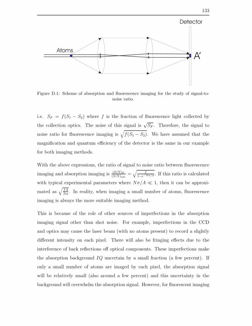
133
Detector
A’Atoms
Figure D.1: Scheme of absorption and fluorescence imaging for the study of signal-to-noise ratio.
i.e. SF = f(S1 − S2) where f is the fraction of fluorescence light collected by
the collection optics. The noise of this signal is√SF . Therefore, the signal to
noise ratio for fluorescence imaging is√
f(S1 − S2). We have assumed that the
magnification and quantum efficiency of the detector is the same in our example
for both imaging methods.
With the above expressions, the ratio of signal to noise ratio between fluorescence
imaging and absorption imaging is (S/N)F
(S/N)abs=√
f1−e−Nσ/A . If this ratio is calculated
with typical experimental parameters where Nσ/A ≪ 1, then it can be approxi-
mated as√
fANσ
. In reality, when imaging a small number of atoms, fluorescence
imaging is always the more suitable imaging method.
This is because of the role of other sources of imperfections in the absorption
imaging signal other than shot noise. For example, imperfections in the CCD
and optics may cause the laser beam (with no atoms present) to record a slightly
different intensity on each pixel. There will also be fringing effects due to the
interference of back reflections off optical components. These imperfections make
the absorption background IQ uncertain by a small fraction (a few percent). If
only a small number of atoms are imaged by each pixel, the absorption signal
will be relatively small (also around a few percent) and this uncertainty in the
background will overwhelm the absorption signal. However, for fluorescent imaging

134
these imperfections will show up only as a small percentage of the total fluorescent
signal, and so will have far less negative influence on the measurement.
Appendix E
Control
We use two computers to run our experiment; one computer controls all of the
timing, digital, analog, and GPIB commands (control computer) while the other is
dedicated to running the camera (camera computer). To initiate an image acqui-
sition, the control computer externally triggers the camera and with the computer
software running, the software takes the images and stores the data in the hard
disk. The control computer subsequently communicates with the camera computer
via serial cable to call the files containing the final image which is then analysed
by a MATLAB program specifically written to calculate various cloud parameters
including temperature and density. Allocating control and acquisition tasks to dif-
ferent computers means that the camera computer can analyze the data from the
previous shot while the control computer moves on to the experimental sequence
for the next shot.
A Bose-Einstein condensation experiment requires precise control of a variety of
components. Most functions require timing resolution on the millisecond scale,
but for certain key tasks like imaging, we need timing with microsecond precision.
There are several basic types of outputs and inputs our control system needs to
handle, namely digital input/output, analog input/output, serial, and GPIB out-
puts. For a schematic of how all these components come together, refer to Figure
E.1. The digital/analogue input/output channels are all provided by three National
135
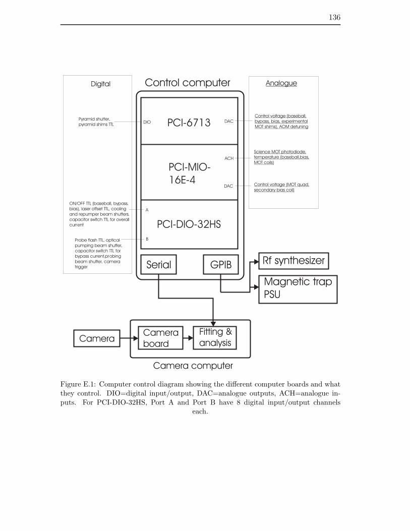
136
PCI-6713
PCI-MIO-
16E-4
PCI-DIO-32HS
DIO
DAC
DAC
ACH
A
B
Pyramid shutter,
pyramid shims TTL
ON/OFF TTL (baseball, bypass,
bias), laser offset TTL, cooling
and repumper beam shutters,
capacitor switch TTL for overall
current
Probe flash TTL, optical
pumping beam shutter,
capacitor switch TTL for
bypass current,probing
beam shutter, camera
trigger
Control voltage (baseball,
bypass, bias, experimental
MOT shims), AOM detuning
Science MOT photodiode,
temperature (baseball,bias,
MOT coils)
Control voltage (MOT quad,
secondary bias coil)
Control computerDigital Analogue
Serial GPIB
Camera computer
Fitting &
analysisCamera
boardCamera
Rf synthesizer
Magnetic trap
PSU
Figure E.1: Computer control diagram showing the different computer boards and whatthey control. DIO=digital input/output, DAC=analogue outputs, ACH=analogue in-puts. For PCI-DIO-32HS, Port A and Port B have 8 digital input/output channels
each.

137
PCI-DIO-32HS
Port A Port B
channel 0: Bias/bypass on/offchannel 1: CMOT offset TTL 2channel 2: CMOT offset TTL 1
channel 3: AOM 3 TTLchannel 4: Cap. Switch: overall current
channel 5: Magnetic trap on/offchannel 6: Shutter 3: Science MOT repumper
channel 7: Shutter 1: Science MOT cooling
channel 0: AOM 1 TTLchannel 1: Shutter 2: Probe/OP on/off
channel 2: CMOT lock box gatechannel 3: Bypass fast input
channel 4: Shutter 4 Probe beam On/Offchannel 5: Cap.switch: bypass current
channel 6:channel 7: Camera trigger
ChannelGro
undPCI-6713 PCI-MIO-16E-4
ACH (ac)AIGR
D
channel 12: 2nd MOT photodiodechannel 13: MOT Temperature
channel 14: Baseball Coil Temperaturechannel 15: Bias Coil Temperature
DIO (di)DGR
D
channel 0:channel 1:
channel 2: Shutter 5: Pyramidchannel 3: Pyramid shims TTL
channel 4:channel 5:channel 6:channel 7:
channel 0:channel 1:channel 2:channel 3:channel 4:channel 5:channel 6:channel 7:
PFI (pf)DGR
Dchannel 0... channel 0...
GPCTR_OUT (gp)
DGRD
GPCTR 0:GPCTR 1:
GPCTR 0:GPCTR 1:
DAC OUT(da)
AOGRD
channel 0: Control voltage, overall current controlchannel 1: Control voltage, primary bias MOSFETs
channel 2: Control voltage, bypass currentchannel 3: Auxiliary Voltagechannel 4: AOM 1 Detuning
channel 5: Science Shims N/Schannel 6: Science Shims E/Wchannel 7: Science Shims U/D
channel 0: MOT Quad Currentchannel 1: Secondary bias coil control
voltage
Total 32 44
Figure E.2: A complete allocation of the channels available on our computer NI boards.
138
Instruments boards (PCI-6713, PCI-MIO-16E-4 and PCI-DIO-32HS). Figure E.2
shows all the channels available on the three cards and what they are used for (not
all channels are used). Most of the experiment is controlled by digital outputs,
which control items such as shutters, rf switches, AOMs and the magnetic trap
itself. Our coils (MOT, magnetic trap, shims) require analogue voltage set points.
We also have several instruments including rf and magnetic trap power supply
that use GPIB as the main mode of communication. Our input ports are used to
monitor the fluorescence level from our MOT and to monitor temperature of our
coils via K-type thermocouples.
Bibliography
[1] M.H. Anderson, J.R. Ensher, M.R. Matthews, C.E. Wieman and E.A. Cor-
nell, Observation of Bose-Einstein Condensation in a Dilute Atomic Vapor,
Science, 269, 198 (1995).
[2] L. Pitaevskii and S. Stringari, Bose-Einstein Condensation, Oxford University
Press, 2003.
[3] J. I. Cirac and P. Zoller, Quantum Computations with Cold Trapped Ions,
Phys. Rev. Lett., 74, 4091 (1995).
[4] C. Monroe, D. M. Meekhof, B. E. King, W. M. Itano and D. J. Wineland,
Demonstration of a Fundamental Quantum Logic Gate, Phys. Rev. Lett., 75,
4714 (1995).
[5] D. Leibfried, B. DeMarco, V. Meyer, D. Lucas, M. Barrett, J. Britton, W.
M. Itano and B. Jelenkovi, Perturbing a persistent current with an external
potential, Nature, 422, 412 (2003).
[6] D. Jaksch, C. Bruder, J.I. Cirac, C.W. Gardiner and P. Zoller, Cold Bosonic
Atoms in Optical Lattices, Phys. Rev. Lett., 81, 3108 (1998).
[7] D. Jaksch, H. J. Briegel, J.I. Cirac, C.W. Gardiner and P. Zoller, Entanglement
of Atoms via Cold Controlled Collisions, Phys. Rev.Lett., 82, 1975 (1999).
[8] M. Greiner, O. Mandel, T. Esslinger, T. W. Hansch and Immanuel Bloch,
Quantum phase transition from a superfluid to a Mott insulator in a gas of
ultracold atoms, Nature, 415, 39 (2002).
139
BIBLIOGRAPHY 140
[9] I. L. Chuang, L. M. K. Vandersypen, X. Zhou, D. W. Leung and Seth Lloyd,
Experimental realization of a quantum algorithm, Nature, 393, 143 (1998).
[10] T. Yamamoto, Yu. A. Pashkin, O. Astafiev, Y. Nakamura and J. S. Tsai,
Demonstration of conditional gate operation using superconducting charge
qubits, Nature, 425, 941 (2003).
[11] S. Kuhr, W. Alt, D. Schrader, M. Mller, V. Gomer and D. Meschede, Deter-
ministic delivery of a single atom, Science, 293, 278 (2001).
[12] J. J. Garcia-Ripoll, P. Zoller and J. I. Cirac, Quantum information processing
with cold atoms and trapped ions, J. Phys. B, 38, 567 (2005).
[13] G. K. Brennen, C. M. Caves, P. S. Jessen, I. H. Deutsch, Quantum Logic
Gates in Optical Lattices, Phys. Rev. Lett, 82, 1060 (1998).
[14] J. Mompart, K. Eckert, W. Ertmer, G. Birkl and M. Lewenstein, Quantum
Computing with Spatially Delocalized Qubits, Phys. Rev. Lett., 90, 147901
(2003).
[15] H. Metcalf., Laser Cooling and Trapping, Springer-Verlag New York Inc., 1999.
[16] E. Arimondo, M. Inguscio, and P. Violino, Experimental determinations of
the hyperfine structure in the alkali atoms, Review of Modern Physics, 49, 31
(1977).
[17] V. Bagnato, D. E. Pritchard, and D. Kleppner., Bose-Einstein condensation
in an external potential., Phys. Rev. A, 35, 4354 (1987).
[18] K. Huang., Statistical Mechanics, Jhon Whiley, 1963.
[19] O.J. Luiten, M.W. Reynolds and J. T. M. Walraven, Kinetic theory of the
evaporative cooling of a trapped gas, Phys. Rev. A, 53, 381 (1996).
[20] P. W. H. Pinkse, A. Mosk, M. Weidemuller, M.W. Reynolds, T.W. Hijmans
and J. T. M. Walraven, Adiabatically Changing the Phase-Space Density of a
Trapped Bose Gas, Phys. Rev. Lett., 78, 990 (1997).

BIBLIOGRAPHY 141
[21] P. W. H. Pinkse, A. Mosk, M. Weidemuller, M.W. Reynolds, T.W. Hijmans
and J. T. M. Walraven, One-dimensional evaporative cooling of magnetically
trapped atomic hydrogen, Phys. Rev. A, 57, 4747 (1998).
[22] J.L. Roberts, N.R. Claussen, Burke, Jr., James P., Chris H. Greene, E.A. Cor-
nell and C.E. Wieman, Resonant Magnetic Field Control of Elastic Scattering
of Cold 85Rb, Phys. Rev. Lett., 81, 5109 (1998).
[23] H. M. J. M Boesten, C.C. Tsai, J.R. Gardner, D.J. Heinzen and B.J. Verhaar,
Observation of a shape resonance in the collision of two cold 87Rb atoms, Phys.
Rev. A, 55, 636 (1997).
[24] Burke, Jr., James P., John L. Bohn, B.D. Esry and Chris H. Greene, Prospects
for Mixed-Isotope Bose-Einstein Condensates in Rubidium, Phys. Rev. Lett.,
80, 2097 (1998).
[25] N. Bogolubov, On the theory of superfluidity, J. Phys., 11, 23 (1947).
[26] W. Ketterle, D.S. Durfee and D.M. Stamper-Kurn. Making, probing and
understanding Bose-Einstein condensates. In S. Stringari M. Inguscio and
C.E. Wieman, editors, Proceedings of the International School of Physics -
Enrico Fermi, page 67. IOS Press, 1999.
[27] T. W. Hansch and A. L. Schawlow, Cooling of gases by laser radiation, Opt.
Commun, 13, 68 (1975).
[28] Steven Chu, L. Hollberg, J.E. Bjorkholm, Alex Cable and A. Ashkin, Three-
Dimensional Viscous Confinement and Cooling of Atoms by Resonance Radi-
ation Pressure, Phys. Rev. Lett., 55, 48 (1985).
[29] J. Prodan and W. Phillips, Chirping the light fantastic - recent NBS atom
cooling experiments, Prog. Quant. Elect., 8, 231 (1984).
[30] W. Ertmer, R. Blatt, J. L. Hall, and M. Zhu, Laser manipulation of atomic
beam velocities: Demonstration of stopped atoms and velocity reversal, Phys.
Rev. Lett., 54, 996 (1985).
BIBLIOGRAPHY 142
[31] R. Watts and C. Wieman, Manipulating atomic velocities using diode lasers,
Opt. Lett., 11, 291 (1986).
[32] V. S. Bagnato, G. P. Lafyatis, A. G. Martin, E. L. Raab, R. N. Ahmad-Bitar,
and D. E. Pritchard, Continuous stopping and trapping of neutral atoms, Phys.
Rev. Lett., 58, 2194 (1987).
[33] W. Phillips and H. Metcalf, Laser deceleration of an atomic beam, Phys. Rev.
Lett., 48, 596 (1982).
[34] P. Lett, W. Phillips, S. Rolston, C. Tanner, R. Watts, and C. Westbrook,
Optical molasses, J. Opt. Soc. Am. B, 6, 2084 (1989).
[35] J. Dalibard and C. Cohen-Tannoudji, Laser cooling below the Doppler limit by
polarization gradients: simple theoretical-models, J. Opt. Soc. Am. B, 6, 2023
(1989).
[36] A. Aspect, E. Arimondo, R. Kaiser, N. Vansteenkiste, and C. Cohen-
Tannoudji, Laser Cooling below the One-Photon Recoil Energy by Velocity-
Selective Coherent Population Trapping, Phys. Rev. Lett, 61, 826 (1988).
[37] Nir Davidson, Heun Jin Lee, Mark Kasevich, and Steven Chu, Raman cooling
of atoms in two and three dimensions, Phys. Rev. Lett., 72, 3158 (1994).
[38] E.L. Raab, M. Prentiss, Alex Cable, Steven Chu and D.E. Pritchard, Trapping
of Neutral Sodium Atoms with Radiation Pressure, Phys. Rev. Lett., 59, 2631
(1987).
[39] K. Lindquist, M. Stephens and C. Wieman, Experimental and theoretical study
of the vapor-cell Zeeman optical trap, Phys. Rev. A, 46, 4082 (1992).
[40] C.G. Townsend, N.H. Edwards, C.J. Cooper, K.P. Zetie, C.J. Foot, A.M.
Steane, P. Szriftgiser, H. Perrin and J. Dalibard, Phase-space density in the
magneto-optical trap, Phys. Rev. A, 52, 1423 (1995).

BIBLIOGRAPHY 143
[41] C.G. Townsend, N.H. Edwards, K.P. Zetie, C.J. Cooper, J. Rink and C.J.
Foot, High-density trapping of cesium atoms in a dark magneto-optical trap,
Phys. Rev. A, 53, 1702 (1996).
[42] C. Monroe, W. Swann, H. Robinson and C. Wieman, Very Cold Trapped
Atoms in a Vapor Cell, Phys. Rev. Lett., 65, 1571 (1990).
[43] F. Shimizu, K. Shimizu, and H. Takuma, Four-beam laser trap of neutral
atoms, Opt. Lett., 16, 339 (1991).
[44] K. Lee, J. Kim, H. Noh, and W. Jhe, Single-beam atom trap in a pyramidal
and conical hollow mirror, Opt. Lett., 21, 1177 (1996).
[45] J. Reichel, W. Hansel, and T. Hansch, Atomic micromanipulation with mag-
netic surface traps, Phys. Rev. Lett., 83, 3398 (1999).
[46] J. Arlt, O. Marago, S. Webster, S. Hopkins, and C. Foot, A pyramidal
magneto-optical trap as a source of slow atoms, Opt. Comm., 157, 303 (1998).
[47] Alan L. Migdall, John V. Prodan, William D. Phillips, Thomas H. Bergeman
and Harold J. Metcalf, First Observation of Magnetically Trapped Neutral
Atoms, Phys. Rev. Lett., 54, 2596 (1985).
[48] V.S. Bagnato, G.P. Lafyatis, A.G. Martin, E.L. Raab, R.N. Ahmad-Bitar and
D.E. Pritchard, Continuous Stopping and Trapping of Neutral Atoms, Phys.
Rev. Lett., 58, 2194 (1987).
[49] H. F. Hess, G. P. Kochanski, J. M. Doyle, N. Masuhara, D. Kleppner and
Thomas J. Greytak, Magnetic Trapping of Spin Polarized Atomic Hydrogen,
Phys. Rev. Lett., 59, 672 (1987).
[50] R. van Roijen, J.J. Berkhout, S. Jaakkola, and J.T.M. Walraven, Experiments
with Atomic Hydrogen in a Magnetic Trapping Field, Phys. Rev. Lett, 61, 931
(1988).

BIBLIOGRAPHY 144
[51] W. Ketterle and D.E. Pritchard, Trapping and focusing ground state atoms
with static fields, Appl. Phys. B, 54, 403 (1992).
[52] E. Majorana, Nuovo Cimento, 9, 43 (1932).
[53] G. Breit and I. I. Rabi, Measurement of nuclear spin, Phys. Rev, 38, 2832
(1931).
[54] Norman F. Ramsey, Molecular Beams, Clarendon Press, 1956.
[55] W. Ketterle and N.J. van Druten, Evaporative Cooling of Trapped Atoms,
Adv. At. Mol. Opt. Phys., 37, 181 (1996).
[56] Walraven. In E. Riis G. L. Oppo, S. M. Barnett and M. Wilkinson, editors,
Quantum Dynamics of Simple Systems, Vol. 44. IOP Bristol, 1996.
[57] G. Rudolf, W. Matthias and Ovchinnikov Yurii B., Optical dipole traps for
neutral atoms, Advances in Atomic, Molecular and Optical Physics, 42,
(2000).
[58] L. Allen, Optical resonance and two-level atoms, Wiley, New York, 1975.
[59] D.M. Stamper-Kurn, M.R. Andrews, A.P. Chikkatur, S. Inouye, H.-J. Mies-
ner, J. Stenger and W. Ketterle, Optical Confinement of a Bose-Einstein
Condensate, Phys. Rev. Lett., 80, 2030 (1998).
[60] M. P. A. Fisher, P. B. Weichman, G. Grinstein and D. S. Fisher, Boson
localization and the superfluid-insulator transition, , 40, 546 (1989).
[61] C. S. Chuu, F. Shreck, T. P. Meyrath, J. L. Hansen, G. N. Price and M. G.
Raizen, Direct observation of sub-Poissonian number statistics in a degenerate
Bose gas, Phys. Rev. Lett, 95, 260403 (2005).
[62] K. Lee, J. Kim, H. Noh, and W. Jhe, Single-beam atom trap in a pyramidal
and conical hollow mirror, Opt. Lett., 21, 1177 (1996).
BIBLIOGRAPHY 145
[63] J. Arlt, P. Bance, S. Hopkins, J. Martin, S. Webster, A. Wilson, K. Zetie and
C.J. Foot, Suppression of collisional loss from a magnetic trap, J. Phys. B,
31, L321 (1998).
[64] Peter Baranowski, Towards number correlated states of a Bose-Einstein con-
densed gas, Undergraduate project report, 2005.
[65] W. Alt, An objective lens for efficient fluorescence detection of single atoms,
Optik., 113, 142 (2002).
[66] W. Alt, D. Schrader, S. Kuhr, M. Muller, V. Gomer and D. Meschede, Single
atoms in a standing-wave dipole trap, Phys.Rev.A, 67, 1033403 (2003).
[67] David E. Pritchard, Proceedings of the 11th International Conference on
Atomic Physics, 619, (1989).
[68] M. E. Gehm, K. M. OHara, T. A. Savard, and J. E. Thomas, Dynamics of
noise-induced heating in atom traps, , 58, 3914 (1998).