Diplomarbeit

Performant Trust andSimilarity Metrics

for Inconsistent Knowledge-bases

Florian Mittag

Dezember 2008

Betreuung: Prof. Dr. Andreas DengelDipl. Inf. Malte Kiesel

Arbeitsgruppe Wissensbasierte SystemeProf. Dr. Andreas Dengel

Technische Universität Kaiserslautern

Fachbereich Informatik

Florian Mittag Kaiserslautern, den 18. Dezember 2008Konrad-Adenauer-Straße 6367663 Kaiserslautern

Erklärung

Hiermit erkläre ich, dass ich die Arbeit selbstständig verfasst und nur die angegebe-nen Hilfsmittel verwendet habe.

(Florian Mittag)

Contents

1 Introduction 11.1 Motivation . . . . . . . . . . . . . . . . . . . . . . . . . . . . . . 11.2 Structure of the thesis . . . . . . . . . . . . . . . . . . . . . . . . 21.3 Prerequisites . . . . . . . . . . . . . . . . . . . . . . . . . . . . . 3

2 Skipforward overview 42.1 Skipinions: The top level ontology . . . . . . . . . . . . . . . . . 52.2 Formal definitions . . . . . . . . . . . . . . . . . . . . . . . . . . 72.3 Maintaining information provenance and authentication . . . . . . 92.4 Item identity . . . . . . . . . . . . . . . . . . . . . . . . . . . . . 102.5 Manual and automatic annotation . . . . . . . . . . . . . . . . . . 112.6 Architecture . . . . . . . . . . . . . . . . . . . . . . . . . . . . . 11

3 Theoretical Foundations 123.1 Trust . . . . . . . . . . . . . . . . . . . . . . . . . . . . . . . . . 12

3.1.1 What is trust? . . . . . . . . . . . . . . . . . . . . . . . . 133.1.2 Personalized views using trust . . . . . . . . . . . . . . . 133.1.3 Trust models . . . . . . . . . . . . . . . . . . . . . . . . 14

3.2 Recommender Systems . . . . . . . . . . . . . . . . . . . . . . . 143.2.1 Collaborative Filtering . . . . . . . . . . . . . . . . . . . 153.2.2 Content-based Filtering . . . . . . . . . . . . . . . . . . . 183.2.3 Hybrids . . . . . . . . . . . . . . . . . . . . . . . . . . . 19

4 Approach 204.1 User similarity . . . . . . . . . . . . . . . . . . . . . . . . . . . 20

4.1.1 Adapting the Pearson correlation . . . . . . . . . . . . . . 214.1.2 Limits of the Pearson correlation . . . . . . . . . . . . . . 234.1.3 The constrained Pearson correlation . . . . . . . . . . . . 244.1.4 Computational complexity and incremental calculation . . 25

4.2 Creating personalized views . . . . . . . . . . . . . . . . . . . . 294.2.1 Confidence in similarities . . . . . . . . . . . . . . . . . 304.2.2 Trust model in Skipforward . . . . . . . . . . . . . . . . 324.2.3 Feature aggregation . . . . . . . . . . . . . . . . . . . . . 32

i

4.2.4 Using domain knowledge to reduce data sparsity . . . . . 33

5 Implementation 365.1 Main algorithms . . . . . . . . . . . . . . . . . . . . . . . . . . . 36

5.1.1 Initializing the similarity values . . . . . . . . . . . . . . 365.1.2 Listening for feature changes . . . . . . . . . . . . . . . . 385.1.3 Incremental update of similarity values . . . . . . . . . . 385.1.4 Inferencing . . . . . . . . . . . . . . . . . . . . . . . . . 41

5.2 Data structures . . . . . . . . . . . . . . . . . . . . . . . . . . . 425.2.1 Feature Cache . . . . . . . . . . . . . . . . . . . . . . . . 425.2.2 Incremental user similarities . . . . . . . . . . . . . . . . 45

6 Evaluation 466.1 Evaluation parameters . . . . . . . . . . . . . . . . . . . . . . . . 466.2 Statistical results . . . . . . . . . . . . . . . . . . . . . . . . . . 466.3 Performance . . . . . . . . . . . . . . . . . . . . . . . . . . . . . 54

7 Summary and Outlook 567.1 Outlook . . . . . . . . . . . . . . . . . . . . . . . . . . . . . . . 56

7.1.1 Optimization of data structures . . . . . . . . . . . . . . . 567.1.2 Relationships between feature types . . . . . . . . . . . . 577.1.3 Handling of non-binary feature types . . . . . . . . . . . 577.1.4 Similarities on partial data sets . . . . . . . . . . . . . . . 58

A Glossary 59

B Proof of equations 61

C Feature types of the evaluation 63

Bibliography 64

ii

Chapter 1

Introduction

1.1 Motivation

Recently, I was making plans for the evening and decided to go to the cinema.Since I was very busy in the days before that, I had paid little attention to themovies that were shown at that time and had only a few hours to choose which oneI wanted to see.

My first source of information about the scheduled movies was the InternetMovie Database (IMDb1), where I could view the average ratings of the movies,user comments and other information like cast and runtime, but there were severalproblems. The ratings are averaged overall opinions that not necessarily reflect theway I would rate those movies. And even if I agreed with the rating of a particularmovie in general, I might not be in the mood for it that night. There are also manydetails about a film that are not contained in the description of the IMDb, e.g., if thestunts are exaggerated or if the humor is silly. These information might be found inuser comments, but then again they can be biased by personal opinions and I don’tknow about my consensus with these.

I then asked some friends for their opinion about aspects of the movie thatI knew we often agreed upon. For example, one of my friends almost alwaysthought of stunts to be exaggerated and unrealistic, so I knew that I could ignorehis comment about this feature. On the other hand, we shared the same sense ofhumor, so his opinion about this aspect was a reliable information to me. However,due to the fact that I had less then a hundred friends and did not have the time toask more than seven, the number of friends I could ask was low compared to thevast amount of people expressing their opinions on the internet.

As can be seen, each source of information has its advantages and disadvan-tages. The internet provides such a large amount of information on almost ev-erything that it often requires a big effort to find relevant ones. This problem isincreased by the large number of collaboratively created knowledge-bases that al-low users to create and modify content or add comments to it. This sometimes

1http://www.imdb.com

1

makes it hard to determine the source of information, which has a large influenceon the trust we put in it.

The “old-fashioned” way of asking friends and like-minds does not offer asplenty of information as the internet, but our personal knowledge about its sourceoften makes the available information much more useful, because we know how tointerpret it.

It would be desirable to have a system that allows users to express their opin-ions about items, such as movies, books and songs, and supports the search forinformation by automatically aggregating possibly contradictory opinions into apersonalized view. As such, the data has to be represented in a machine-readableformat and has to provide provenance information.

Skipforward is a system that is being developed to meet this criteria. It alreadyallows different users to make machine-readable statements about certain items,while maintaining provenance information. However, it is currently not capableof determining the relevance of information based on previous experience. Theavailable information has to be interpreted differently for each user to turn theminto personalized information.

The basic idea of this thesis is to automatically calculate similarities betweenpairs of users for different topics based on previously expressed opinions. Thesesimilarities are then used to estimate the relevance of information for a specific userto create a personalized view. Since the number of items and opinions about themwill grow during the usage of the system, the algorithms for this calculation aredesigned to work incrementally and still perform efficiently on large knowledge-bases.

1.2 Structure of the thesis

Chapter 2 introduces Skipforward, a framework for distributed, collaborative, andpersonalized annotation of resources with structured metadata. The format ofstored data will be described, as it is the foundation for the later examination ofsimilarity measures and for the algorithms developed.

In Chapter 3, formal definitions of trust are discussed, as they can be usedto describe trustworthiness of information and their sources. After that, a shortoverview on recommender systems is given and important terms and algorithmsare defined and explained.

Based on this knowledge, Chapter 4 elaborates different algorithms to calculateuser similarities with regard to performance and usefulness of their results. Theaggregation of inconsistent information into a personalized view is then realizedusing a formal trust model.

The integration of the developed components into the Skipforward system isdescribed in Chapter 5. To ensure the performance of the algorithms, certain re-quirements have to be made to the underlying data structures.

An evaluation of the implementation with real data concerning music annota-

2

tion is presented in Chapter 6. At first, it is explained how the data was gatheredand what difficulties arise from the nature of its domain. Based on this data theresults of the developed algorithms are examined with respect to their plausibilityand time performance.

Chapter 7 summarizes the results of this thesis and gives an outlook on furtherwork and research that has to be done for this topic.

1.3 Prerequisites

The reader should be familiar with the idea of the Semantic Web and in particularwith RDF/S2 and URIs. Although it is not necessary to be familiar the Web 2.0and tagging, experience with collaborative platforms like Wikis, interactive onlinedatabases and recommendation services is helpful in order to get a full grasp of theproblems and methods of resolution presented in this thesis.

Skipforward and the algorithms described in this thesis are implemented inJava 53 using the Jena4 framework. Knowledge of object-oriented programming isnecessary for the understanding of the source code.

2http://www.w3.org/RDF/3http://java.sun.com/4http://jena.sourceforge.net/

3

Chapter 2

Skipforward overview

As already mentioned in Section 1.1, the number of services on the internet offeringinformation about a certain topic is overwhelming. For the area of music alone,there are many different platforms that all focus on different aspects of music.Many of these services also include webradios, where people can listen to the musicimmediately, and webshops to buy the discovered music.

For example, Discogs1 is a “community-built database of music information”that provides discographies for artists and labels, detailed information about re-leases, and reviews.

Last.fm2 on the other hand focuses on music recommendation based on thelistening behavior of its users, but also offers the possibility to add user-definedtags, comments, and descriptions to artists and songs.

Pandora3 also focuses on music recommendation, but does so by comparingsongs through their content, which has been added by professional music-analystsdescribing the features of a song.

So, why would one like to extend the vast list of competing services with yetanother one, dispersing the available information to more locations than they al-ready are?

The motivation behind Skipforward is to assists the user in his search for rele-vant and reliable information [Kiesel and Schwarz, 2008]. He should not have toread through fifty user comments to eventually find the information he was look-ing for. When there are different opinions about something, the user should beprovided with additional information about the reliability of statements, making iteasier for him to decide on his own what to believe.

Some platform allow users to add tags to items to describe them. However,often the only way to state that a certain tag is not suitable for an item is to not addthis tag. Other users can not distinguish if a tag was not added on purpose or if itwas forgotten.

1http://www.discogs.com/2http://www.last.fm/3http://www.pandora.com/

4

The system should not be limited to a certain type of features, like songs, but beeasily extensible to other areas. Also, the information provided by the user shouldstay within his reach, as they may be personal and users may not want to feed acentral server with a profile of themselves.

Thus, the requirements made for Skipforward can be summarized into the foll-wing aspects:

Formalization The information and opinion about items of different kinds (songs,movies, etc.) has to be formalized and stored in a machine-readable format,so that it can be used to create useful visualizations that can be easily per-ceived.

Dissent Users should be able to explicitly express their dissens with an opinion ofanother user. This also includes the capability to not only state that an itemhas a certain feature, but also that it does not have a certain feature.

Confidence Sometimes one is not completely sure about a feature of an item, sousers should also be able to express their confidence in their own opinions.This way, others have more information to decide on the reliability of a state-ment.

Decentralized storage Not everyone wants to share his opinions with all otherusers for different reasons. Also, having the data of all users in one location- being controlled by a single person or organization - increases the risk ofmalicious usage of these personal data. Therefore, the system has to be adecentralized network.

Easy merging of databases With the data being stored in a decentralized manner,the effort to merge the databases of different users has to be kept low.

Provenance Because different information have different origins, at every mo-ment it has to be clear where a piece of information comes from. Being ableto safely identify the author of a comment or opinion also increases trust inthe system.

2.1 Skipinions: The top level ontology

Skipforward stores the items and their features in an RDF model and formalizationis realized by its toplevel ontology, called Skipinions, which provides the two basicclasses: Item and Feature.

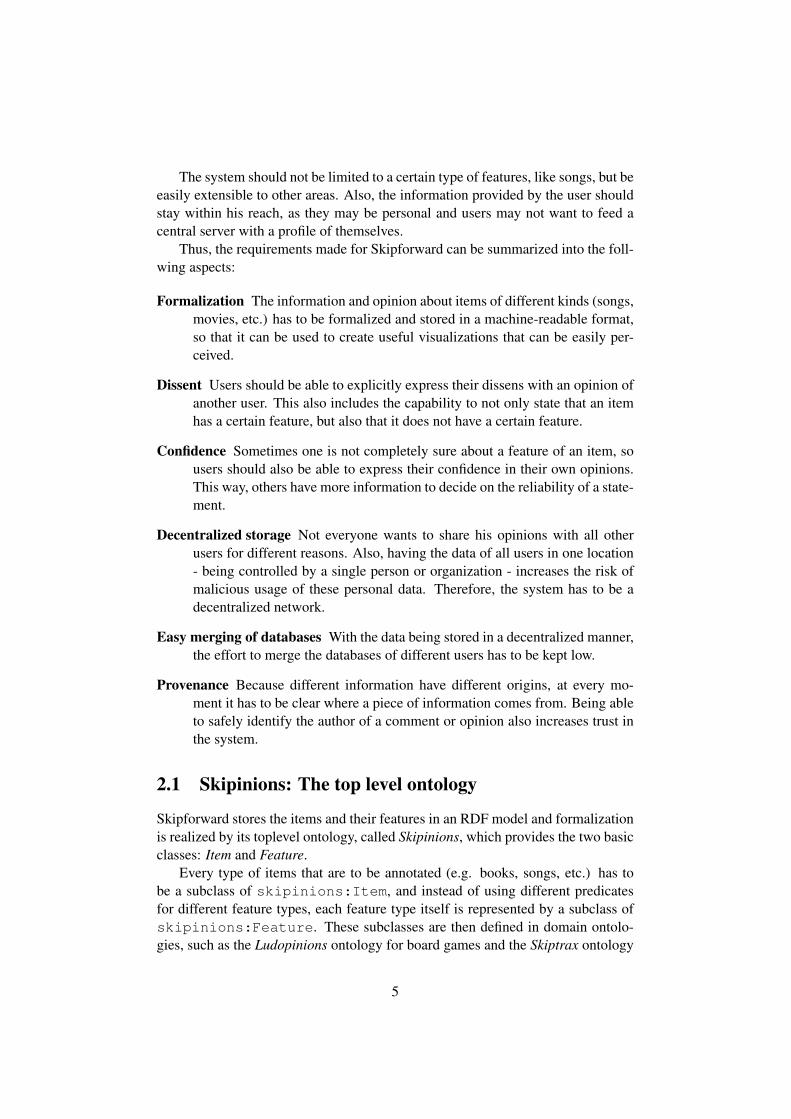
Every type of items that are to be annotated (e.g. books, songs, etc.) has tobe a subclass of skipinions:Item, and instead of using different predicatesfor different feature types, each feature type itself is represented by a subclass ofskipinions:Feature. These subclasses are then defined in domain ontolo-gies, such as the Ludopinions ontology for board games and the Skiptrax ontology

5

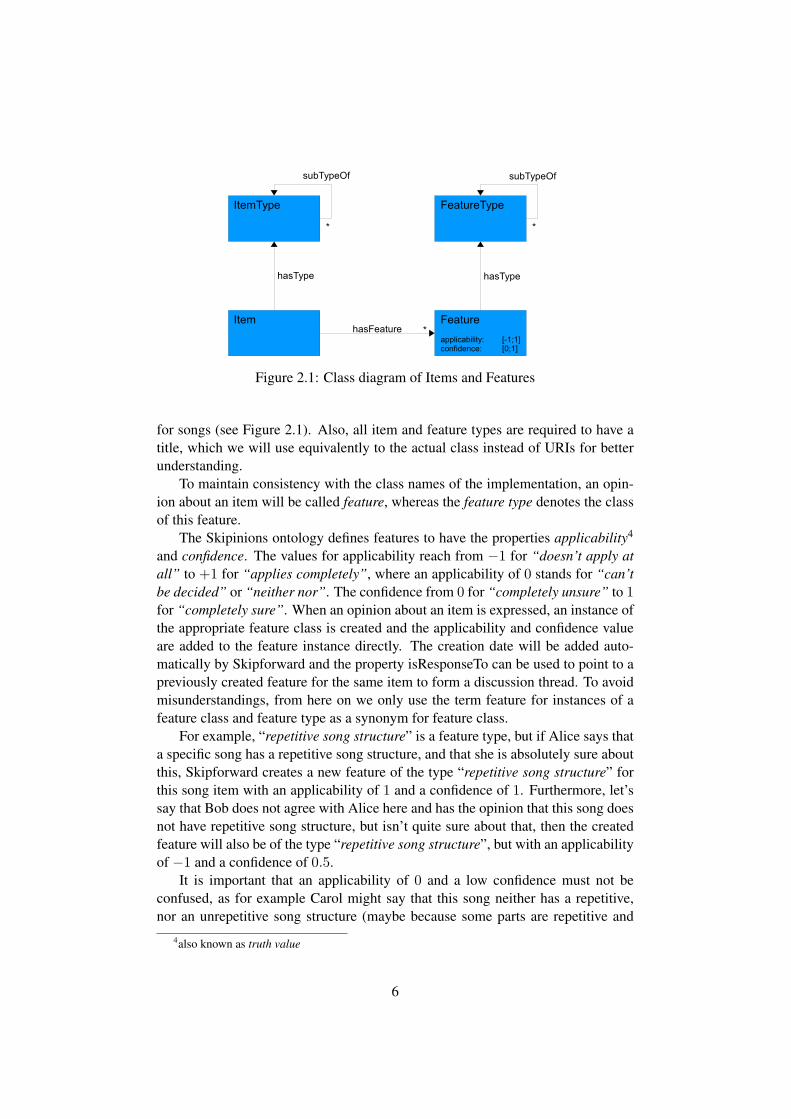
Figure 2.1: Class diagram of Items and Features

for songs (see Figure 2.1). Also, all item and feature types are required to have atitle, which we will use equivalently to the actual class instead of URIs for betterunderstanding.

To maintain consistency with the class names of the implementation, an opin-ion about an item will be called feature, whereas the feature type denotes the classof this feature.

The Skipinions ontology defines features to have the properties applicability4

and confidence. The values for applicability reach from −1 for “doesn’t apply atall” to +1 for “applies completely”, where an applicability of 0 stands for “can’tbe decided” or “neither nor”. The confidence from 0 for “completely unsure” to 1for “completely sure”. When an opinion about an item is expressed, an instance ofthe appropriate feature class is created and the applicability and confidence valueare added to the feature instance directly. The creation date will be added auto-matically by Skipforward and the property isResponseTo can be used to point to apreviously created feature for the same item to form a discussion thread. To avoidmisunderstandings, from here on we only use the term feature for instances of afeature class and feature type as a synonym for feature class.

For example, “repetitive song structure” is a feature type, but if Alice says thata specific song has a repetitive song structure, and that she is absolutely sure aboutthis, Skipforward creates a new feature of the type “repetitive song structure” forthis song item with an applicability of 1 and a confidence of 1. Furthermore, let’ssay that Bob does not agree with Alice here and has the opinion that this song doesnot have repetitive song structure, but isn’t quite sure about that, then the createdfeature will also be of the type “repetitive song structure”, but with an applicabilityof −1 and a confidence of 0.5.

It is important that an applicability of 0 and a low confidence must not beconfused, as for example Carol might say that this song neither has a repetitive,nor an unrepetitive song structure (maybe because some parts are repetitive and

4also known as truth value

6

others are not), but is completely confident about this, would result in a featurewith applicability 0 and confidence 1.

There are of course feature types where applicability values other than 1 or −1seem to do not make much sense, for example for the feature type “lyrics”, becauseeither there are lyrics or not. Then again, some users might think otherwise, so therange of the applicability value is never restricted by the system.

So far, this definition of feature classes only allows one to state whether aspecific feature is present in an item or not, which is why they are called binaryfeatures. Obviously, there can be only one valid feature per user, item and featureclass, meaning that a second feature of the same class, from the same user and tothe same item would make the old feature invalid, which reflects a change in theopinion of the user.

Additionally, subclasses of skipinions:Feature can have an extraslot for defining an object to the feature, like it is needed for the artist orthe title of a song, and are called non-binary features . One basic examplefor a non-binary feature class is already defined in the Skipinions ontology:skipinions:ItemName. The ItemName feature class has an additional prop-erty called itemName that holds a string value. For example, Alice says that a songhas the title “James Bond - Goldeneye (Main Theme)” and is quite sure about it,which results in a feature of type skipinions:ItemName with applicability 1 andconfidence 0.7, and the title as itemName property.

Bob disagrees and on his part expresses the opinion that the song title is simply“Goldeneye” and he is very certain of it, leading to a feature with applicability andconfidence 1 and the string “Goldeneye” as value for the property itemName. Onthe other hand, he thinks that the title Alice gave this song item is not completelywrong, so he also creates a feature of type skipinions:ItemName with theitemName “James Bond - Goldeneye (Main Theme)” with applicability 0.5 andconfidence 1. Note, that Bob’s second opinion is a dissent with Alice’s opinion,not with his own first opinion, because the value of skipinions:itemNamespecializes the feature type.

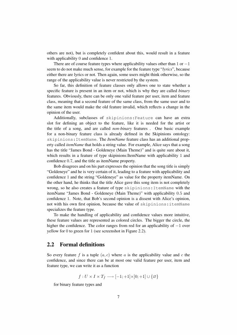
To make the handling of applicability and confidence values more intuitive,these feature values are represented as colored circles. The bigger the circle, thehigher the confidence. The color ranges from red for an applicability of −1 overyellow for 0 to green for 1 (see screenshot in Figure 2.2).

2.2 Formal definitions

So every feature f is a tuple (a, c) where a is the applicability value and c theconfidence, and since there can be at most one valid feature per user, item andfeature type, we can write it as a function

f : U × I × Tf −→ [−1; +1]×]0; +1] ∪ {∅}

for binary feature types and

7

Figure 2.2: Screenshot of the web-interface of Skipforward

f : U × I × Tf ×Otf −→ [−1; +1]×]0; +1] ∪ {∅}

for non-binary feature types, where the involved sets are:

U : set of all usersI: set of all itemsTf : set of all feature typesOtf : set of allowed objects for feature type tf

and ∅ means undefined. For reasons of readability and convenience, we willwrite a feature as variable with indices:

f(u, i, tf )equiv= fu,i,tf = (a, c)

f(u, i, tf , o)equiv= fu,i,tf ,o = (a, c)

with i ∈ I, u ∈ U, tf ∈ Tf and o ∈ Otf

If it is clear from the context that the equations are applied to single featuretypes each, these indices will also be omitted:

f(u, i)equiv= fu,i = (a, c)

8

2.3 Maintaining information provenance and authentica-tion

Every running Skipforward instance represents a node in the peer-to-peer network,which can be started on the user’s own computer or run on a different machine thatprovides access through a web-interface. The user has to enter his XMPP 5 accountinformation and the node then connects to the XMPP server. The nodes commu-nicate with each other by requesting updates and sending updates via XMPP mes-sages and file transfers.

When opinions are expressed by creating instances of feature classes, likeall RDF resources they are identified using a URI. Skipforward encodes theprovenance of skipinions ontology instances as the namespace that is usedto create the resources: Every item or feature is created in the namespaceskip://user@host/, where user@host is the users Jabber ID. Furthermore,each user only creates or modifies statements in his own namespace, which wedefine here as statements whose subject resource is in his own namespace.

Suppose Alice and Bob have the Jabber accounts alice@skipforward.netand bob@skipforward.net respectively, then Alice’s namespace wouldbe skip://alice@skipforward.net/ and Bob’s would beskip://bob@skipforward.net/. If Alice now wants to get the opin-ions of Bob, i.e. the feature instances he created with all their relations, she hasto ask him to send him his private model. Bob will then send his private modelvia XMPP file transfer to Alice, who in turn will only accept statements in Bob’snamespace. That way, Alice knows that all statements in Bob’s namespace werereceived from Bob, or rather from a node that successfully authenticated withBob’s account information to the XMPP server [Wang and Vassileva, 2003]. Allthe private models of different users can be integrated into one big world modelwhile one still can easily determine the provenance of statements.

The ontologies, Skipinions as well as domain ontologies, are distributed usingthe same mechanism. This is possible because ontologies can be in user names-paces, too. For example, seeder@skipforward.net is a valid XMPP account andserves as a seeder for the Skipinions ontology, which is defined in the correspond-ing namespace skip://seeder@skipforward.net/. Users can also definetheir own ontology in their own namespace and it will get distributed to the othernodes the same way the items and features get distributed. On the other hand, cre-ating own accounts with the sole purpose of seeding ontologies is a good way toseparate personal opinions from ontologies. This dummy users do not need to bepermanently logged in into the Skipforward system, but they are the best way topropagate changes on the seeded ontologies as well as new ontologies.

5http://xmpp.org/

9

2.4 Item identity

The consequence of these strictly separated namespaces is that every user can onlyadd features to items that are in his own namespace, too.

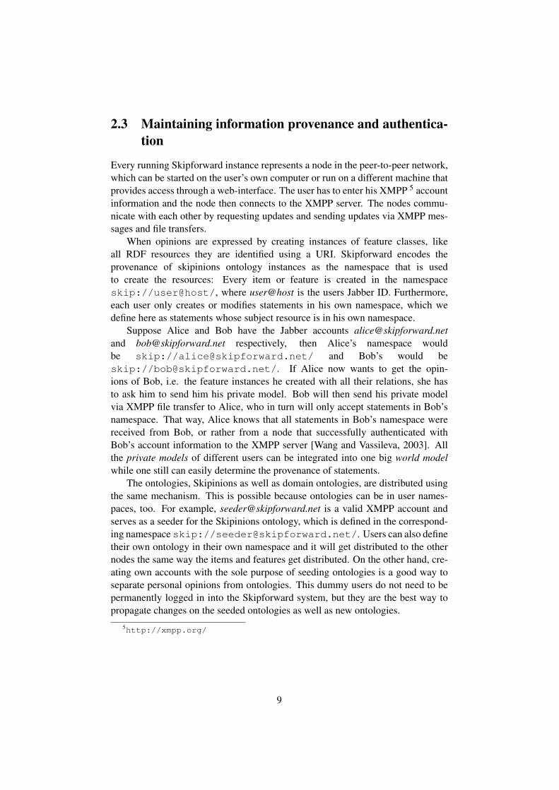
If Alice now wants to state an opinion about one of Bob’s items, there ap-pears to be a problem, because although she would create an instance of the de-sired feature type in her own namespace, the RDF triple relating it to the itemwould have a subject that is NOT in her namespace. The solution is to use theskipinions:isIdenticalTo property6: Alice creates an item in her ownnamespace, relates it to Bob’s item using this predicate and then can express opin-ions about this item in her own namespace (see Figure 2.3).

Figure 2.3: Identical items in different namespaces

When the copy of Bob’s item is created in Alice’s namespace, the name of theitem will also be copied by creating a new ItemName feature in Alice’s namespacewith the same string for the name. This is due to two reasons:

Firstly, if another user, Carol, is a friend of Alice, but not of Bob, she onlysees the items and features in Alice’s and her own namespace. If Alice has notexpressed an opinion about the name of that item, Carol will only see an item withno name. Secondly, if the name in Bob’s namespace would get deleted for somereason, Alice would be left with an item without a name. Copying the name alongwith the item increases the redundancy in the network and therefore makes it morerobust.

The isIdenticalTo relation is transitive, so if Carol copies an item from Alicethat she has previously copied from Bob, it is clear that Carol means the same itemas Bob.

6skipinions:isIdenticalTo is similar to the owl:sameAs property of the Web Ontol-ogy Language (OWL)

10

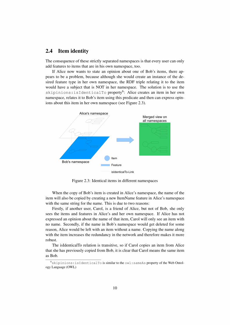
Figure 2.4: Architecture of Skipforward

2.5 Manual and automatic annotation

The items in the database of Skipforward are added by the users while working withthe system. Without any knowledge about the features of an item it can neithercontribute to the user profile nor can its usefulness be estimated, so the featureshave to be added by the users manually, too. This approach can obviously beimpractical and heavily depends on the number and motivation of the people usingthe system. However, for multimedia data, such as audio and video streams, theautomatic extraction of features is sometimes hard to apply, especially for featuresthat are disputable (e.g. mood, genre, etc.). The manual annotation of items oftenlacks alternatives.

On the other hand, using software to automatically extract certain kinds of fea-tures and add them to the Skipforward database is not prohibited in any way andcan provide useful information [Liu et al., 1998]. They will not be discussed fur-ther, though, as this thesis focuses on similarity and trust in a personalized context.

2.6 Architecture

Access to the data is done via the FactsDatabase component of Skipforward in anobject-oriented manner, encapsulating the classes of the skipinions ontology andtheir instances as java classes and object respectively.

Of course, Alice and Bob do not manipulate the data on the RDF triple level.Skipforward provides an object-oriented interface for data manipulation on the ab-straction level of items and features. In the above examples, Alice and Bob will bepresented some graphical user interface that displays the items and their featuresand offers possibilities to add new ones to the database. Things like copying itemsto the own namespace and linking it with its source are handled outside the user’ssight, and requesting and sending updates of private models happens automatically.

11

Chapter 3

Theoretical Foundations

Let us assume that Skipforward is used by many highly motivated people, whofilled the database with thousands or even millions of items, and that there areuseful ontologies for describing almost every aspect of an item with hundreds offeature types. Each item has been annotated by multiple users and they commentedtheir opinions. Even under the optimistic assumption that there are no unhelpfulflamewars between users, it would be unrealistic to expect all users to have thesame opinion about the features of items.

When browsing through the items and viewing their features types, just dis-playing all features of all users or showing arithmetic means of all features wouldnot be a personalized view and probably not very helpful, either. Information thatmight be useful to the user is obscured in two ways:

Firstly, the descriptions of the items may be inconsistent, making it hard toestimate their features at first glance. Secondly, the items that one considers usefulwill most likely represent only a little fraction of the available data, otherwise itwould be sufficient to browse through the items one-by-one.

Considering the inconsistency of data, one intuitive approach is to estimatethe trustworthiness of the information provided by other users. To be able to usethese trust information in algorithms, a formal model needs to be defined. Section3.1 gives an overview of different definitions and shows models of trust and theirformalization.

A well-established method to filter relevant information out of large databasesin a personalized way are recommendation systems. Section 3.2 gives an introduc-tion into the two large classes of recommendation systems, namely collaborativefiltering and content-based filtering.

3.1 Trust

The concept of trust can be applied in different situations: If we want to travel byplane, we wouldn’t do so if we didn’t have trust in the abilities of the pilot and theground personal responsible for the maintenance of the aircraft. If we don’t lock

12

our office when we fetch a cup of coffee, we do so because we trust the other peoplein the department to not go in there and steal our stuff. When one is confronted withcontradicting statements, distinguishing the “right” information from the “wrong”is question of trust.

3.1.1 What is trust?

Obviously, there are different kinds of trust and not all of them are suitable for ourscenario of finding relevant information. [Gutscher et al., 2008, p. 51] defines trustas a multi-relational concept:

“A truster trusts a trustee (e.g., a person, an institution or a techni-cal system) in a certain context, if the truster has confidence1 in thecompetence and intention of the trustee and therefore beliefs that thetrustee acts and behaves in an expected way, which does not harm thetruster.”

Then, trust is distinguished into two categories:

Competence trust Trust in the capability of a person, in an institutionor in the functionality of a machine or a system.

Intentional trust Trust in the moral integrity (benevolence) of a per-son.

In the context of Skipforward, the competence of another user is his ability toprovide correct information and his moral integrity means that he will not inten-tionally provide incorrect information. Since in this case, both the lack of compe-tence and malevolence would lead to incorrect information, when we talk of trustwe mean competence trust, where intentional trust is a special case of it. More de-tailed classifications of different kinds of trust can be found [Jøsang et al., 2007],but are not of interest in the context of this thesis.

3.1.2 Personalized views using trust

As stated at the beginning of this chapter, a simple approach of handling manydifferent opinions about an item would be to calculate the arithmetic mean of allfeatures of a type for an item and just use this mean value. But if one had theopinion that a song has “great lyrics” and the majority of the other users wouldthink the opposite, this arithmetic mean wouldn’t be of much help. There is alsothe problem that people might have a different understanding of the meaning of afeature type, which is a problem of ontology misunderstanding. This is outside thescope of this thesis and we assume that all users implicitly agree on the conceptsrepresented in the ontologies.

1Although the terms trust and confidence are often used synonymous, they are not exactly thesame [Adams, 2005].

13

Assuming a user, Alice, knows that the features about “great lyrics” assignedby another user, Bob, often differ from her own opinion, then Bob’s competence ofdescribing items with the feature type “great lyrics” would be very low relative toAlice. So Alice could decide to generally decrease the influence of Bob’s opinionabout this feature type, i.e. the features of this type. At the same moment, Bob hasthe same reason to have little trust in Alice describing songs with this feature type,because from his point of view she is often wrong.

3.1.3 Trust models

It is possible to model trust values using only one scale. This scale may be discrete(e.g., “no trust”, “some trust”, “full trust”) or continuous (e.g., [0;1] as in [Maurer,1996] or [-1;1] as in [Marsh et al., 1995]), where the exact meaning of the valuesdiffers from model to model. Most existing approaches to model trust not onlyallow to express the degree of trust, but also the degree of certainty or confidencein this trust statement. This can be done by adding a second scale for confidence,similar to the confidence of features in Skipforward, or by representing trust by anupper and a lower bound [Shafer, 1976].

The importance of a confidence value becomes clear when one has to assigna trust value to someone he has little information about. To be secure, one couldalways assign the lowest possible trust value to minimize the risk of false informa-tion, but this could also mean that valuable information are not considered becauseof missing trust. A common solution in this case is to express ignorance, whichmeans that one lacks sufficient information and therefore has no confidence in themade trust statement.

Although continuous scales for trust and confidence values allow more detailedtrust statements than discrete scales, they also make it hard to define clear semanticsfor them [Gutscher et al., 2008]. For example, a confidence value of 1 is twice asbig as 0.5, but does not necessarily mean that the confidence is twice as big. It isalso unclear if a confidence value of 0.8 means the same to different users, whereasthe extreme values 0 and 1 can safely be assumed to mean the same to everyone2.

3.2 Recommender Systems

Recommender systems emerged in the mid-1990s and have become an importantarea in research and industry [Schafer et al., 1999], because they main goal is tohelp users deal with information overload. Online shops, like Amazon.com3, usecollaborative filtering techniques to recommend products to the customer that hemight find interesting, based on the products other customers bought previously[Linden et al., 2003], other platforms like Last.fm4 recommend artists and songs

2Of course, the same holds for the trust values.3http://www.amazon.com/4http://www.last.fm

14

based on the listening behavior of their users.The recommendation problem can be commonly described as the problem of

estimating the utility of an item to a user, that he has not seen or rated, yet. Theitems with the highest estimated usefulness will then be presented to him. Thisestimation is based on ratings previously given by this user to other items andfurther information, depending on the type of the recommendation system. Oftenthe user can assign the ratings manually, but it can also be implicitly gathered, e.g.,by monitoring his shopping or listening behavior.

It should be noted that the term rating is often used to describe how the userrates the utility of an item. Because in most recommender systems user can onlygive an overall rating, rating and utility are often used synonymously.

Formally, the estimated usefulness can be seen as a function

pred : U × I −→ R (3.1)

where U is the set of all user, I the set of all items and R is a totally orderedset. As mentioned earlier, different recommender systems have different methodsof predicting the usefulness and use different data for it.

3.2.1 Collaborative Filtering

Collaborative filtering (CF) systems first calculate the similarity between all pairsof users based on the co-rated items, i.e., items that have been rated by both users,and denotes the highly similar users as peers or neighbors. The highest rated itemsof these neighbors that are not already rated by the active user, i.e., the user cur-rently interacting with the system, are then recommended to him. The assumptionbehind this behavior is that users who rated the same items similarly have similartaste and, hence, the rating of new item will be similar to those of similar users[Sarwar et al., 2000].

Since the recommendations are based on the similarity of users, this method iscalled user-based CF. Another method is to calculate the similarity between itemsand then recommend items that are similar to the ones already rated highly. Twoitems are considered similar, if they received similar ratings from the same users(e.g., users who like item A also like item B and users who don’t like item A alsodon’t like item B). A popular example for item-based CF are the recommendationsfrom Amazon.com: “Users who bought A also bought B.”

It should be noted that the only information used about the items is their ratingsfrom different users, no information about their content is needed. The ratingscan be stored in a so-called user-item matrix, where rows are users and columnsare items (see Figure 3.1). A column now represents all ratings by all users forthis particular item, whereas rows represent all ratings of all items of a specificuser. Calculating the similarity of users or items can thus be seen as a comparisonbetween rows or columns respectively, which both can be interpreted as vectors.

Additionally, CF algorithms can be divided into two general classes, memory-based and model-based. As the name suggests, model-based CF tries to learn a

15

Figure 3.1: User-Item Matrix where two users are compared.

model of the user from the collected ratings and calculates its predictions basedon this model. Memory-based CF utilizes the entire user-item matrix and usesheuristics to calculate similarities. In [Sarwar et al., 2001], the classes memory-based and user-based are assumed equal, same with model-based and item-based,but there are also model-based methods that are user-based [Adomavicius andTuzhilin, 2005].

The Pearson correlation

A common measure used in CF is the Pearson product-moment correlation coef-ficient, or Pearson correlation coefficient for short, as it measures the linear re-lationship between two random variables X and Y . It can be interpreted as thenormalized covariance of both random variables [Rodgers and Nicewander, 1988]and is of range [−1; +1]:

ρX,Y =cov(X,Y )√var(X)var(Y )

(3.2)

=E[(X − E(X))(Y − E(Y ))]√

(X − E(X))2(Y − E(Y ))2

If it is calculated from a sample of these random variables, it is written as:

rX,Y =

n∑i=1

(xi − x)(yi − y)√n∑

i=1(xi − x)2

n∑i=1

(yi − y)2(3.3)

16

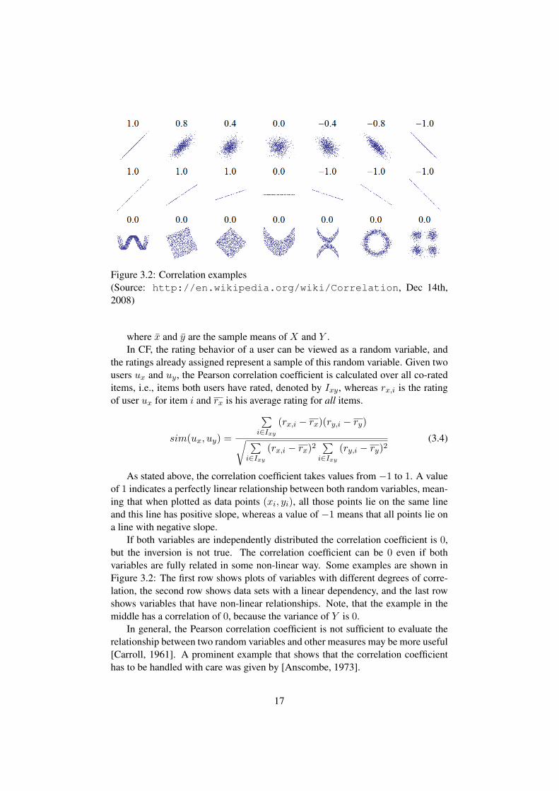
Figure 3.2: Correlation examples(Source: http://en.wikipedia.org/wiki/Correlation, Dec 14th,2008)

where x and y are the sample means of X and Y .In CF, the rating behavior of a user can be viewed as a random variable, and

the ratings already assigned represent a sample of this random variable. Given twousers ux and uy, the Pearson correlation coefficient is calculated over all co-rateditems, i.e., items both users have rated, denoted by Ixy, whereas rx,i is the ratingof user ux for item i and rx is his average rating for all items.

sim(ux, uy) =

∑i∈Ixy

(rx,i − rx)(ry,i − ry)√ ∑i∈Ixy

(rx,i − rx)2∑

i∈Ixy

(ry,i − ry)2(3.4)

As stated above, the correlation coefficient takes values from −1 to 1. A valueof 1 indicates a perfectly linear relationship between both random variables, mean-ing that when plotted as data points (xi, yi), all those points lie on the same lineand this line has positive slope, whereas a value of −1 means that all points lie ona line with negative slope.

If both variables are independently distributed the correlation coefficient is 0,but the inversion is not true. The correlation coefficient can be 0 even if bothvariables are fully related in some non-linear way. Some examples are shown inFigure 3.2: The first row shows plots of variables with different degrees of corre-lation, the second row shows data sets with a linear dependency, and the last rowshows variables that have non-linear relationships. Note, that the example in themiddle has a correlation of 0, because the variance of Y is 0.

In general, the Pearson correlation coefficient is not sufficient to evaluate therelationship between two random variables and other measures may be more useful[Carroll, 1961]. A prominent example that shows that the correlation coefficienthas to be handled with care was given by [Anscombe, 1973].

17

4

6

8

10

12

14

4 6 8 10 12 14 16 18 20

y1

x1

4

6

8

10

12

14

4 6 8 10 12 14 16 18 20

y2

x2

4

6

8

10

12

14

4 6 8 10 12 14 16 18 20

y3

x3

4

6

8

10

12

14

4 6 8 10 12 14 16 18 20

y4

x4

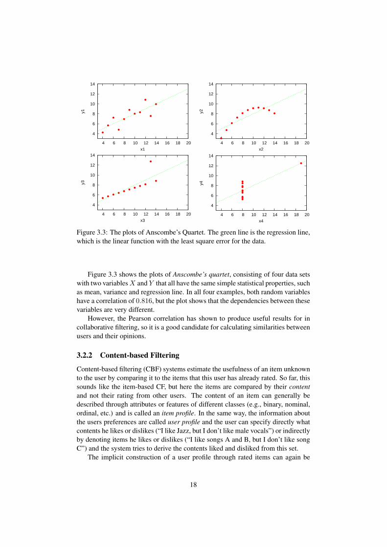
Figure 3.3: The plots of Anscombe’s Quartet. The green line is the regression line,which is the linear function with the least square error for the data.

Figure 3.3 shows the plots of Anscombe’s quartet, consisting of four data setswith two variablesX and Y that all have the same simple statistical properties, suchas mean, variance and regression line. In all four examples, both random variableshave a correlation of 0.816, but the plot shows that the dependencies between thesevariables are very different.

However, the Pearson correlation has shown to produce useful results for incollaborative filtering, so it is a good candidate for calculating similarities betweenusers and their opinions.

3.2.2 Content-based Filtering

Content-based filtering (CBF) systems estimate the usefulness of an item unknownto the user by comparing it to the items that this user has already rated. So far, thissounds like the item-based CF, but here the items are compared by their contentand not their rating from other users. The content of an item can generally bedescribed through attributes or features of different classes (e.g., binary, nominal,ordinal, etc.) and is called an item profile. In the same way, the information aboutthe users preferences are called user profile and the user can specify directly whatcontents he likes or dislikes (“I like Jazz, but I don’t like male vocals”) or indirectlyby denoting items he likes or dislikes (“I like songs A and B, but I don’t like songC”) and the system tries to derive the contents liked and disliked from this set.

The implicit construction of a user profile through rated items can again be

18

divided into the two classes memory-based (or heuristic-based), where rated itemsare directly compared to the unrated items, and model-based techniques, that learna model from the rated items that will be used to predict the usefulness of unrateditems, such as artificial neuronal networks or decision trees.

3.2.3 Hybrids

Although each of the approaches described above can be applied on their own,there are many kinds of recommendation systems that use some kind of combina-tion of both filtering methods or other approaches not listed here [Balabanovic andShoham, 1997]. The aim is to compensate disadvantages of one kind of systemsby integrating techniques of the other one.

For example, if there are not enough co-rated items to calculate user similaritiesin a collaborative system, content profiles can be used to find similar users, thusallowing to overcome the sparsity problem [Pazzani, 1999].

Keeping this in mind, when we use the terms CF or CBF, we refer to the “pure”idea without any combination or augmentation with other methods.

19

Chapter 4

Approach

The basic idea of this thesis is to create a personalized view of the inconsistentdata by automatically calculating a similarity between pairs of users, based on theexisting annotations stored in the database. The user similarity is then transformedinto a competence trust value to determine the influence another user’s annotationsshould have on the aggregated view of the item [Massa and Avesani, 2004].

In Section 4.1 we will first examine how collaborative filtering systems calcu-late their user similarity values and then derive an algorithm that works with thedata provided by Skipforward with respect to computational performance. Basedon this results, in Section 4.2.2 a trust model is developed to represent the compe-tence trust in other users that is used to create a personalized view on data [Zieglerand Lausen, 2004].

4.1 User similarity

Because user-based CF also calculates the similarity between users based on the ex-isting data, it is reasonable to assume that CF algorithms provide a good foundationfor calculating user similarities for content-based data. We decided to concentrateon the Pearson correlation, as it is widely applied in collaborative recommendationsystems and it is known to yield good results.

As stated earlier, the difference between content-based and collaborative filter-ing is that CF only considers one value per user and item, the rating, whereas incontent-based filtering there are multiple values per item and these values can alsobe of different type. Skipforward can be seen as a hybrid system, because there aremultiple values per item like in CBF, but they are contributed by the users and maybe subjective and inconsistent like in CF (see Table 4.1).

The idea here is to apply the Pearson correlation on one feature type at a time,which will result in a correlation coefficient that describes how similar two usersare regarding this specific feature type. To reduce complexity, we will ignore non-binary feature types in this diploma thesis.

20

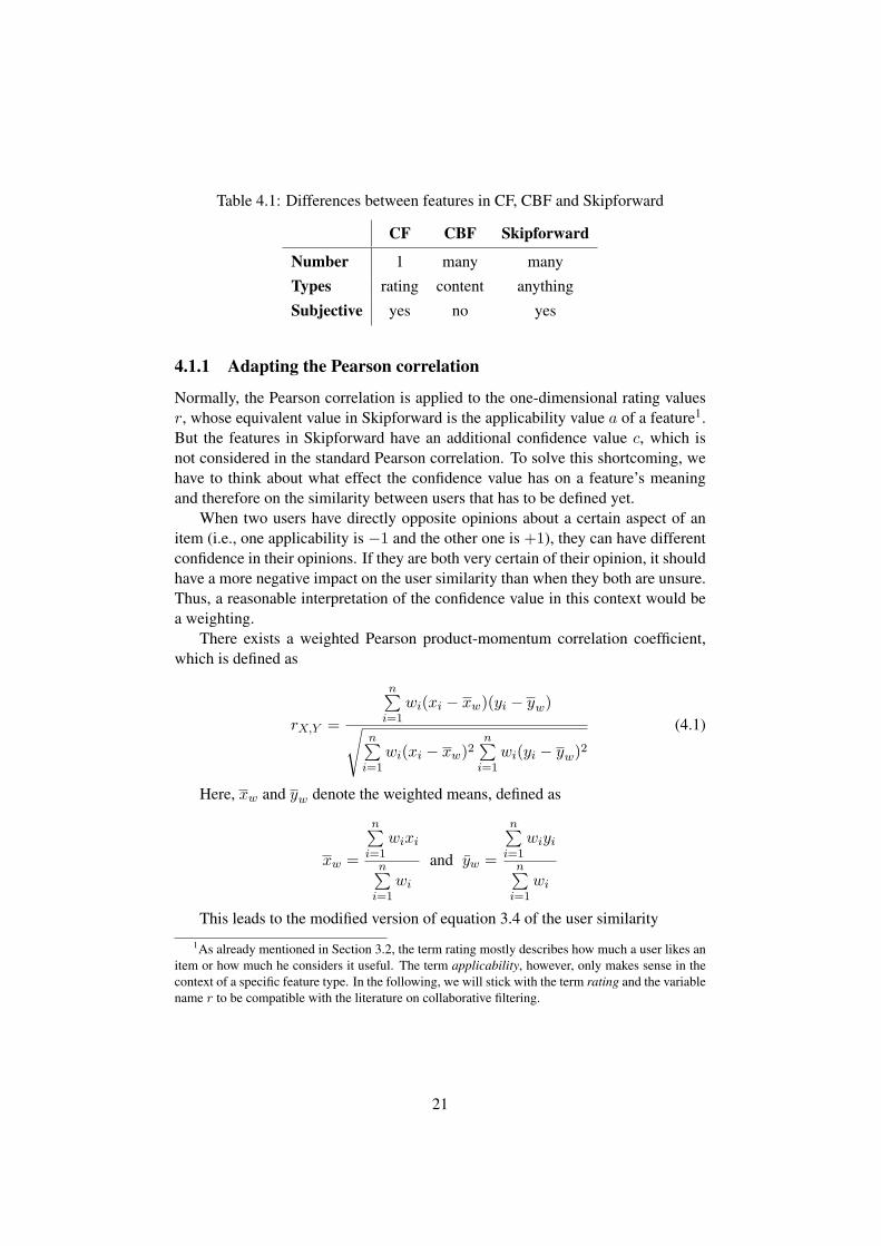
Table 4.1: Differences between features in CF, CBF and Skipforward

CF CBF Skipforward

Number 1 many many

Types rating content anything

Subjective yes no yes

4.1.1 Adapting the Pearson correlation

Normally, the Pearson correlation is applied to the one-dimensional rating valuesr, whose equivalent value in Skipforward is the applicability value a of a feature1.But the features in Skipforward have an additional confidence value c, which isnot considered in the standard Pearson correlation. To solve this shortcoming, wehave to think about what effect the confidence value has on a feature’s meaningand therefore on the similarity between users that has to be defined yet.

When two users have directly opposite opinions about a certain aspect of anitem (i.e., one applicability is −1 and the other one is +1), they can have differentconfidence in their opinions. If they are both very certain of their opinion, it shouldhave a more negative impact on the user similarity than when they both are unsure.Thus, a reasonable interpretation of the confidence value in this context would bea weighting.

There exists a weighted Pearson product-momentum correlation coefficient,which is defined as

rX,Y =

n∑i=1

wi(xi − xw)(yi − yw)√n∑

i=1wi(xi − xw)2

n∑i=1

wi(yi − yw)2(4.1)

Here, xw and yw denote the weighted means, defined as

xw =

n∑i=1

wixi

n∑i=1

wi

and yw =

n∑i=1

wiyi

n∑i=1

wi

This leads to the modified version of equation 3.4 of the user similarity1As already mentioned in Section 3.2, the term rating mostly describes how much a user likes an

item or how much he considers it useful. The term applicability, however, only makes sense in thecontext of a specific feature type. In the following, we will stick with the term rating and the variablename r to be compatible with the literature on collaborative filtering.

21

sim(ux, uy) =

∑i∈Ixy

wi(rx,i − rx)(ry,i − ry)√ ∑i∈Ixy

wi(rx,i − rx)2∑

i∈Ixy

wi(ry,i − ry)2(4.2)

with

I: set of all itemsIx = {i ∈ I|rx,i 6= ∅}: set of all items rated by user ux

Iy = {i ∈ I|ry,i 6= ∅}: set of all items rated by user uy

Ixy = Ix ∩ Iy: set of all items rated by user ux and uy

But this equation still doesn’t fit our purpose, because it allows only one weightvalue per rating value to be defined, meaning that the ratings of both users have tobe weighted with the same weight value wi. It might seem possible to have twodifferent weight values in the denominator, a weight wx,i for the variance of userux and a weight wy,i for the variance of user uy, but the numerator only contains asingle weight value for both the rating value of user ux and uy.

We looked into the possibility to use two different weight values wx,i and wy,i

in the denominator and a combined weight value wxy,i in the numerator. If thecombined weight fulfills some criteria, it is possible to prove that the resultingcorrelation coefficient still has a range of [−1; +1], but it would be necessary toexamine if the resulting equation still has the properties of a correlation. If onlyone combined weight value wxy,i is used in the equation, it is the normal weightedPearson correlation and we do not need to worry about its properties. We decidedto consider both variants in our algorithm and compare their results based on eval-uation data.

In both cases, we need to find a function to calculate a combined weight valueout of the weight values from both users. The choice of this function is not arbi-trary, as the combined weight has to reasonably represent the combination of twoconfidences. Desired properties are:

• The confidence value is of range [0; +1], so the combined weight/confidenceshould be, too.

• If one of the users is completely unsure of his opinion (i.e., a confidence of0), the similarity of the corresponding rating should not be considered (i.e.,a combined weight value of 0).

• If both users have the same amount of confidence in their opinion (i.e., thesame confidence value), the combined weight value should be the same.

Two candidates for calculating the combined weight that fulfill these criteriaare

22

wxy,i := min(cx,i, cy,i) (4.3)

wxy,i :=√cx,icy,i (4.4)

where (4.3) is the minimum of both weights and (4.4) their geometrical mean.The weight values wx,i and wy,i are defined as

wx,i := cx,i

wy,i := cy,i (4.5)

if we want to use user-specific weight values in the denominator and

wx,i = wy,i := wxy,i (4.6)

if we use only the combined weight value for the weighted Pearson correlation,which will then look like this:

sim(ux, uy) =

∑i∈Ixy

wxy,i(rx,i − rx)(ry,i − ry)√ ∑i∈Ixy

wx,i(rx,i − rx)2∑

i∈Ixy

wy,i(ry,i − ry)2(4.7)

with the weighted mean defined as

rx =

∑i∈Ix

wx,irx,i∑i∈Ix

wx,iand rx =

∑i∈Iy

wy,iry,i∑i∈Iy

wy,i(4.8)

4.1.2 Limits of the Pearson correlation

An often instanced advantage of the Pearson correlation is that it produces use-ful results even if the two compared sample sequences have different ranges. Incollaborative filtering systems, the range of rating values out of which users canchoose is usually the same for every user, e.g., a discrete scale from 1 to 10, but theusers may still use only parts of this range as ratings. Alice might only rate itemswith values from 3 to 10, whereas Bob rates items from 1 to 8. For the Pearsoncorrelation it makes no difference if the two users could not use other values or ifthey just did not use them, which leads to a behavior that is desirable in the contextof CF. As an example, imagine Alice rated item A with 5 and item B with 10, andBob rated the same items with 1 and 3, then the Pearson correlation coefficient forthose two users is exactly 1. Why is that?

The Pearson correlation centers the rating values to 0 when calculating thevariance and covariance. The mean rating of Alice is 2, the mean rating of Bobis 7.5, which means that for both items both users differ from their mean rating

23

into the same direction, i.e., a rating less than the mean or a rating greater than themean. Both users rated item B higher than item A, which leads to a correlation of+1, because the Pearson correlation indicates the strength of a linear relationship(see Chapter 3.2.1). Between only two points, a connecting line can always beplotted, so unless one of the two variables (i.e., the ratings of one user) has novariance because both values are the same, the correlation will always be +1 or−1.

If the strategy of a collaborative filtering algorithm is to recommend the highestranked items of the neighbors (i.e., the users with the highest similarity) then it doesnot matter if the other user’s ratings have a different range, because only the relativeordering of his items is important. In Skipforward, however, we don’t want to getthe item with the highest applicability for a certain feature type, but to predict thepersonal opinion about the applicability of a feature type for a specific item basedon the features other users assigned to it.

The sparsity of data is common problem for recommendation systems[O’Donovan and Smyth, 2005], [Massa and Bhattacharjee, 2004], especially fornew users, because the system does not have enough data to compare the otherusers with the new one. In conjunction with the usage of the Pearson correlation,this problem can increase in Skipforward because of the lack of variance in theapplicability of some feature types. If, for example, the first couple of songs thenew user has annotated do not have a flute solo, all features of type “flute solo” headded will most likely have an applicability value of −1, which means they haveno variance because they are equal to the mean value of −1. But the normal Pear-son correlation requires variance in at least one of the two random variables if thecorrelation is to be defined and non-zero (see equation (4.2)). So although mostother users may agree with him in the applicability of the feature type “flute solo”in all of the annotated songs, the calculated correlation will be not defined or zero.

With an increasing amount of annotations made, the probability of having vari-ance in all feature types increases and the problem vanishes. But users often judgethings by their first impression, so we have to find a way to provide useful predic-tions as soon as possible.

4.1.3 The constrained Pearson correlation

In [Shardanand and Maes, 1995], a variant of the Pearson correlation is introducedthat takes the positivity and negativity of ratings into account, which they called“Constrained Pearson r Algorithm”. They used a discrete scale of rating valuesfrom 1 to 7 in their recommender system “Ringo”, where values greater than 4represent a positive and values below 4 a negative rating. The desired behavior ofthe constrained Pearson correlation is that it only increases if the two users rated anitem both positive or both negative, so instead of subtracting the mean from eachrating, the neutral value 4 is subtracted.

The neutral value of the applicability of features in Skipforward is 0, so wesubstitute the (ri − r) terms with (ri − 0) or simply ri:

24

i rx,i ry,i normal constrained

1 1.0 1.0 0.00 1.00

2 0.0 1.0 0.00 0.71

3 -1.0 0.0 0.87 0.50

4 -1.0 -1.0 0.82 0.67

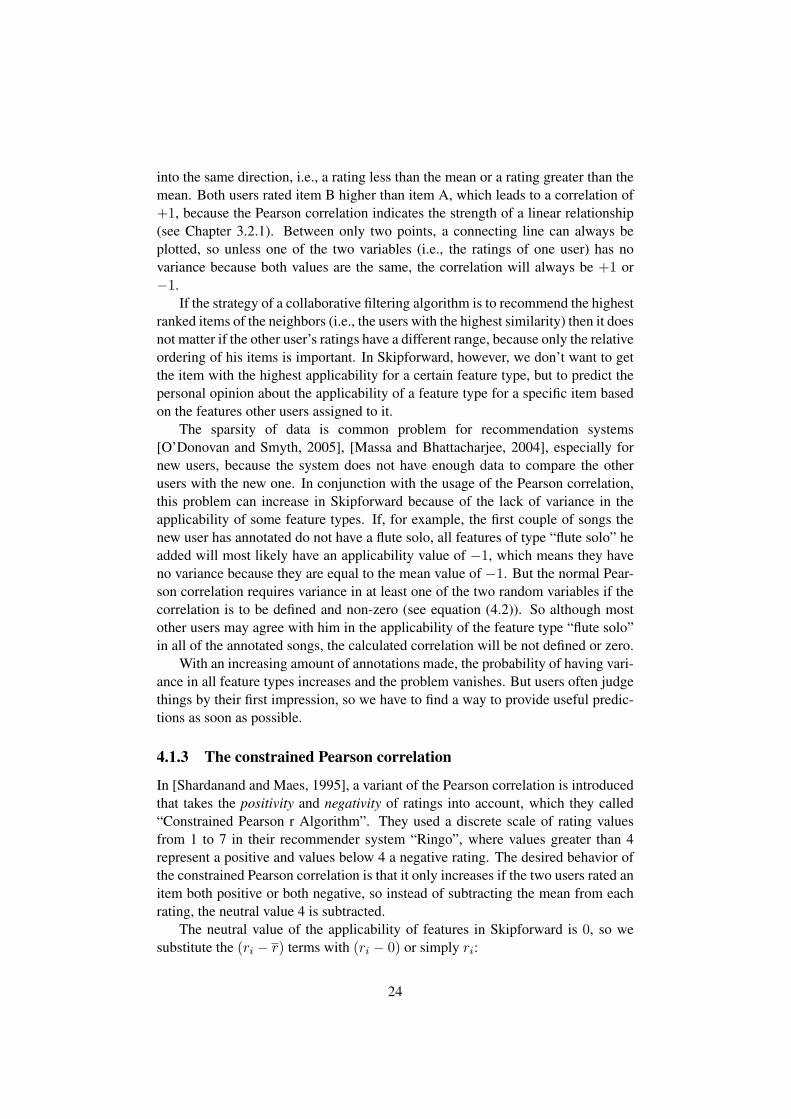
Table 4.2: Example results for both correlation variants. The weights for all ratingsare set to 1 here for simplification.

sim(ux, uy) =

∑i∈Ixy

wxy,i(rx,i − 0)(ry,i − 0)√ ∑i∈Ixy

wx,i(rx,i − 0)2∑

i∈Ixy

wy,i(ry,i − 0)2

=

∑i∈Ixy

wxy,irx,iry,i√ ∑i∈Ixy

wx,i(rx,i)2∑

i∈Ixy

wy,i(ry,i)2(4.9)

Another advantage of the constrained algorithm is that one commonly rateditem is sufficient for a correlation that is non-zero (if the ratings are non-zero, ofcourse), which means that user similarities can be detected earlier than with thestandard Pearson correlation, which needs at least two commonly rated items.

An example calculation can be seen in Table 4.2: In each line the correlationsare calculated using only the ratings of this item and previous ones (e.g., the cor-relation in line 2 only include the ratings for item 1 and 2). The normal Pearsoncorrelation coefficient is undefined (and therefore set to 0) in the first line, becauseit needs at least two ratings to be defined, and in the second line, because there isno variance in the ratings of user uy. However, the constrained Pearson correlationalready shows reasonable result with only one item being co-rated.

An evaluation conducted with “Ringo” showed that in its case the constrainedPearson r algorithm performed best, both in that it was able to provide predictionsin more cases and that these predictions were more accurate than the normal Pear-son r algorithm [Shardanand and Maes, 1995]. However, since we intend to usethese algorithms in a very different scenario, the assumption that these results holdfor Skipforward, too, has to be proven in an evaluation.

4.1.4 Computational complexity and incremental calculation

All of the above mentioned variants of the Pearson correlation can be implementedstraight forward: For each user ux, the correlation with each of the other users hasto be calculated based on the features of items they both have annotated.

25

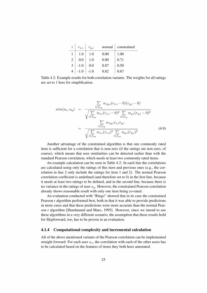
Algorithm 4.1.1: CALCULATEALLCORRELATIONS(tf )

for each ux ∈ Ufor each uy ∈ U

do CalculateCorrelation(ux, uy, tf )

If there are m users and n items, then there are m(m−1)2 correlations to be cal-

culated and each calculation has to examine at most n items, so this naive approachhas a computational complexity of O(m2n). The correlation values will be validas long as no new ratings are submitted or existing ones are updated. In the eventof a change in the ratings of user ux, his correlation coefficients to each of the otherm− 1 users has to be recalculated, which has a complexity of O(mn).

In collaborative recommender systems, user similarities are used to find goodrecommendations based on similar users and usually do not change significantlyin a short time. So instead of recalculating the correlation coefficients every timea user asks for a recommendation, many systems with a large number of user anditems often recalculate all user similarities once in a while, because the impactof few changes onto the recommendation process itself is often too negligible tojustify a permanently updated user similarity matrix [Adomavicius and Tuzhilin,2005].

Skipforward has a bit different requirements, because the purpose of user sim-ilarities is not only to help the system make recommendations, but to provide apersonalized view while browsing through the items. Additionally, Skipforwardis a decentralized system where every user has his own node in the network2 andcommunicates only with the nodes in his roster (his friends). As a consequence,every node has to calculate the user similarities himself, but only needs to do so forthe similarity between the own user and each of his friends, not between the friends.So if a user has m friends, the costs for computing the correlation coefficients forall of his friends are in O(mn).

An approach to reduce the computational costs of maintaining the user simi-larities is presented in [Papagelis et al., 2005], by updating the similarity values ifa rating has changed instead of recalculating them from scratch. For example, ifthere are n′ rated items and a new weighted rating rx,a for item a is submitted, theupdate of the weighted mean of ratings of user ux would look like this:

r′x =

n′+1∑i=1

wx,irx,i

n′+1∑i=1

wx,i

=

n′∑i=1

wx,irx,i + wx,arx,a

n′∑i=1

wx,i + wx,a

=

(n′∑

i=1wx,i

)rx + wx,arx,a

n′∑i=1

wx,i + wx,a

(4.10)2Even if multiple Skipforward nodes run on the same machine or even in the same Java VM, they

are still separated instances and communicate only through XMPP messages and filetransfers.

26

As this example shows, instead of iterating over all n items with a complex-ity of O(n), the new weighted mean r′x can be calculated by updating the old

weighted mean rx in constant time O(1), if rx and the old sum of weightsn′∑

i=1wx,i

are cached. In the same way, the correlation coefficients can be updated with anconstant effort per changed rating, leading to a complexity of O(m) for updatingthe user similarities to m− 1 other users.

Unfortunately, the equation for calculating the correlation is more complexthan the equation for the weighted mean, which makes it even more difficult todefine an incremental update for it. The basic idea of [Papagelis et al., 2005] tosimplify this problem is to split equation (3.4) into three factors B, C, and D:

sim(ux, uy) = A =B√C√D

=

∑i∈Ixy

(rx,i − rx)(ry,i − ry)√ ∑i∈Ixy

(rx,i − rx)2√ ∑

i∈Ixy

(ry,i − ry)2(4.11)

Instead of updating the correlation with a single rule, increments e, f and g aredetermined to update each of this factors independently. The new correlation A′ isthen easily computed using the new factors B′, C ′ and D′:

A′ =B′√C ′√D′

=B + e√

C + f√D + g

(4.12)

Since we want to implement different variants of the Pearson correlation anduse weighted rating, we can only use this basic idea and have to deduce our ownupdate rules.

For reasons of better readability, we will differ from the notation used so far.The following variables are used:

xi, yi ratings of users ux and uy for item i, respectivelywx,i, wy,i weights of the ratings of users ux and uy for item i, respectivelywxy,i combined weight of both users ux and uy

x, y weighted mean of all ratings of users ux and uy, respectively

The Pearson correlation from equation (4.1) is therefore split into the threefactors

B =∑i∈Ixy

wxy,i(xi − x)(yi − y)

C =∑i∈Ixy

wx,i(xi − x)2 (4.13)

D =∑i∈Ixy

wy,i(yi − y)2

27

The active item is the item whose rating has changed. Furthermore, primedvariables denote the new value after the update to distinguish them from the oldvalues:

xa, wx,a the old rating and its weight of the active itemx′a, w′x,a the new rating and its weight of the active itemx′ new weighted mean of all ratings of user ux

The difference between new and old values is defined as

dxa = x′a − xa ⇔ x′a = xa + dxa

and analogously for dx and dwa.There are three different kinds of changes in ratings: A new rating can be added

and an existing one can be modified or deleted. Since every rating is weighted,adding a new rating or deleting an old rating can be interpreted as a change of anexisting rating by modifying its weight from zero to non-zero or vice versa.

[Papagelis et al., 2005] also distinguish between the two cases of the other userhaving also rated the active item or not. Because the sums in the equation onlyaccumulate ratings of co-rated items, in the latter case only mean rating of theactive user changes, requiring less computations than if the set of co-rated itemschanges.

However, since we use weighted ratings and these weights may be defined as acombination of the confidences of both users, the change of a rating of user ux canalso effect the weighted mean of user uy. Thus, we only need to consider one caseand therefore need to deduce only one set of update rules3 for B, C and D:

B′ = B + dwxy,a(x′a − x′)(ya − y) + wxy,adxa(ya − y) (4.14)

− dx(∑i∈Ixy

wxy,iyi − y∑i∈Ixy

wxy,i)

C ′ = C + dwx,a(x′a − x′)2 + 2wx,adxa(xa − x′) + wx,adx2a (4.15)

− 2dx(∑i∈Ixy

wx,i − x∑i∈Ixy

wx,i) + dx2∑i∈Ixy

wx,i

D′ = D + dwy,a(ya − y)2 (4.16)

At first glance, this update rules can not be calculated in constant time, becausethey contain factors that need to be summed over items. The solution is to cachethat elements of the equation so that no iterations over items has to be made. These

3The derivation of this update rules is given in Appendix B.

28

elements have to be updated, too, but this is a rather trivial task and will not beexplained further.

Values that need to be cached for this updates are:

• B, C, Dthe factors to calculate A′ (for each pair of users)

• x, ythe weighted means of all ratings (for each user)

•∑

i∈Ix

wx,i,∑i∈Iy

wy,i

the total weight of all ratings (for each user)

•∑

i∈Ixy

wxy,ixi ,∑

i∈Ixy

wxy,iyi

the wxy,i-weighted sum of ratings for co-rated items (for each pair of users)

•∑

i∈Ixy

wx,ixi ,∑

i∈Ixy

wy,iyi

the wx,i/wy,i-weighted sum of ratings for co-rated items (for each pair ofusers)

•∑

i∈Ixy

wxy,i

the total combined weight for all co-rated items (for each pair of users)

•∑

i∈Ixy

wx,i,∑

i∈Ixy

wy,i

the total weight for all co-rated items (for each pair of users)

The mean can also be updated incrementally, but we can generalize equation(4.10), which can only be used if a new rating is added, to a form that updates themean if an existing rating is modified.

r′x =

(∑i∈Ix

wx,i

)x− wx,axa + w′x,ax

′a∑

i∈Ix

wx,i − wx,a + w′x,a

(4.17)

If a rating is added or deleted this equation can also be used with w′x,a or wx,a

set to 0.

4.2 Creating personalized views

In collaborative filtering systems, user similarities can easily be used to make ratingpredictions for items that the user has not rated yet [Adomavicius and Tuzhilin,2005]. When a user browses items in Skipforward, the personalized view should

29

not only include a prediction of his opinion about a feature type that he has notexpressed yet, but should also aggregate the features assigned by the other usersfor feature types he already stated an opinion. We therefore use the more generalterm feature aggregation and view the feature prediction function as a special usecase of it.

Often, only the ratings of the most similar users are included, which is denotedby U . Some examples are:

rx,i =1|U |

∑uy∈U

ry,i simple mean (4.18a)

rx,i = k∑

uy∈U

sim(ux, uy)ry,i weighted mean (4.18b)

rx,i = rx + k∑

uy∈U

sim(ux, uy)(ry,i − ry) adjusted weighted mean (4.18c)

where k =1∑

uy∈U

sim(ux, uy)normalization factor

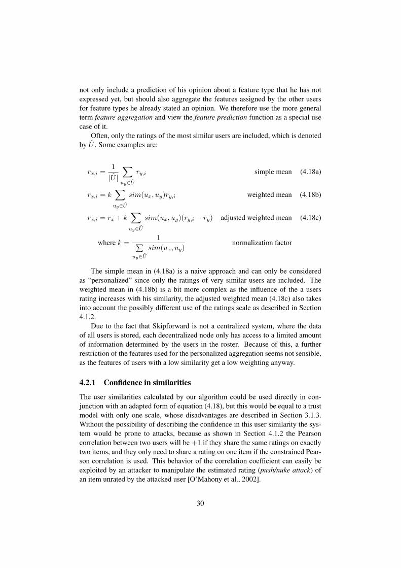
The simple mean in (4.18a) is a naive approach and can only be consideredas “personalized” since only the ratings of very similar users are included. Theweighted mean in (4.18b) is a bit more complex as the influence of the a usersrating increases with his similarity, the adjusted weighted mean (4.18c) also takesinto account the possibly different use of the ratings scale as described in Section4.1.2.

Due to the fact that Skipforward is not a centralized system, where the dataof all users is stored, each decentralized node only has access to a limited amountof information determined by the users in the roster. Because of this, a furtherrestriction of the features used for the personalized aggregation seems not sensible,as the features of users with a low similarity get a low weighting anyway.

4.2.1 Confidence in similarities

The user similarities calculated by our algorithm could be used directly in con-junction with an adapted form of equation (4.18), but this would be equal to a trustmodel with only one scale, whose disadvantages are described in Section 3.1.3.Without the possibility of describing the confidence in this user similarity the sys-tem would be prone to attacks, because as shown in Section 4.1.2 the Pearsoncorrelation between two users will be +1 if they share the same ratings on exactlytwo items, and they only need to share a rating on one item if the constrained Pear-son correlation is used. This behavior of the correlation coefficient can easily beexploited by an attacker to manipulate the estimated rating (push/nuke attack) ofan item unrated by the attacked user [O’Mahony et al., 2002].

30

A user similarity based on hundred items should weigh more than one onlybased on two ratings, so the confidence in the user similarity should therefore bebased on the amount of underlying data that led to the similarity value. Possiblemeasures are:

confsim1(ux, uy) =|Ixy||I|

(4.19a)

confsim2(ux, uy) =2|Ixy||Ix|+ |Iy|

(4.19b)

confsim3(ux, uy) =|Ixy||Ix ∪ Iy|

(4.19c)

The ratio of common rated items to all items in (4.19a) depends on the totalnumber of items in the database and leads to mostly low confidence values. (4.19b)and (4.19c) depend on the number of items that have been rated by at least one ofthe two users. Some example values are shown in Table 4.3.

Again, if the confidence values in Skipforward are interpreted as weights, theequations can be modified to make certain features count more than uncertain ones:

confsim(ux, uy) =

∑i∈Ixy

wxy,i

|I|(4.20a)

confsim(ux, uy) =

2∑

i∈Ixy

wxy,i∑i∈Ix

wx,i +∑i∈Iy

wy,i(4.20b)

Equation (4.19c) can not be adapted that easily, because it is hard to definewhat weights have to be used for the items of |Ix ∪ Iy|. Since the weights are ofrange [0; +1], it is clear that in (4.20a) the confidence confsim ∈ [0; +1], too, andthe same can be shown for equation (4.20b).

Table 4.3: Comparison of trust-confidence measures. Total number of items is1000, ratios are rounded to 3 decimals

|Ix| |Iy| |Ixy| confsim1 confsim2 confsim3

10 10 10 0.01 1 110 100 10 0.01 0.182 0.1100 100 10 0.01 0.1 0.053100 100 50 0.05 0.5 0.333100 100 100 0.1 1 1

31

Luckily, the sums used in this definitions of the confidence in user similarityare already calculated during the incremental update of the correlation itself, so thecomputational complexity here is also only in O(1).

4.2.2 Trust model in Skipforward

The trust model we use in Skipforward is very similar to the model used for fea-tures, so the competence trust in another user can be seen as a non-binary featuretype, where the applicability is equivalent to the user similarity and the confidencehas the same meaning4. But in contrast to the applicability value, which has arange of [−1; 1], we limit the range of the competence trust to non-negative values.The trust of user ux in user uy regarding features of type tf can be described as afunction

trust : U × U × Tf −→ [0; 1]× [0; 1]

that maps every pair of users and a feature type to a trust value consisting ofthe raw competence trust and the confidence.

trust(ux, uy, tf ) 7−→ (comp(ux, uy, tf ), conf (ux, uy, tf )) (4.21)

There are different possibilities to map the user similarity sim with range[−1; 1] to the desired range of [0; 1], which is why we introduce a new functioncomp that can be defined in different ways to allow more control over the mapping,for example:

comp(ux, uy, tf ) = max(0, sim(ux, uy, tf )) (4.22a)

comp(ux, uy, tf ) =(sim(ux, uy, tf ) + 1)

2(4.22b)

In definition of the competence trust value in (4.22a) user similarities below0 are simply interpreted as 0, whereas in (4.22b) the interval [−1; 1] is uniformlymapped to the interval [0; 1], so that a user similarity of 0 still leads to a competencetrust value of 0.5.

4.2.3 Feature aggregation

We define the feature aggregation function for a specific feature type tf of a userux as:

4A special domain ontology, called Skippies ontology, that allows expressing opinions aboutusers, such as trust and other features, is under development and will be added in a future version ofSkipforward.

32

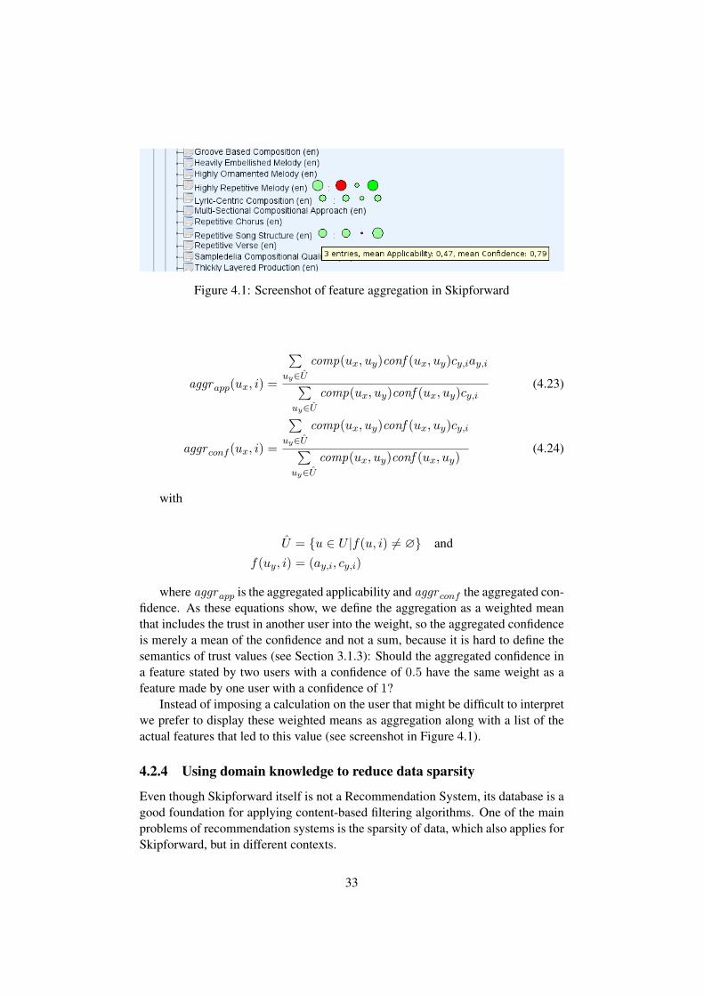
Figure 4.1: Screenshot of feature aggregation in Skipforward

aggrapp(ux, i) =

∑uy∈U

comp(ux, uy)conf (ux, uy)cy,iay,i∑uy∈U

comp(ux, uy)conf (ux, uy)cy,i(4.23)

aggr conf (ux, i) =

∑uy∈U

comp(ux, uy)conf (ux, uy)cy,i∑uy∈U

comp(ux, uy)conf (ux, uy)(4.24)

with

U = {u ∈ U |f(u, i) 6= ∅} and

f(uy, i) = (ay,i, cy,i)

where aggrapp is the aggregated applicability and aggr conf the aggregated con-fidence. As these equations show, we define the aggregation as a weighted meanthat includes the trust in another user into the weight, so the aggregated confidenceis merely a mean of the confidence and not a sum, because it is hard to define thesemantics of trust values (see Section 3.1.3): Should the aggregated confidence ina feature stated by two users with a confidence of 0.5 have the same weight as afeature made by one user with a confidence of 1?

Instead of imposing a calculation on the user that might be difficult to interpretwe prefer to display these weighted means as aggregation along with a list of theactual features that led to this value (see screenshot in Figure 4.1).

4.2.4 Using domain knowledge to reduce data sparsity

Even though Skipforward itself is not a Recommendation System, its database is agood foundation for applying content-based filtering algorithms. One of the mainproblems of recommendation systems is the sparsity of data, which also applies forSkipforward, but in different contexts.

33

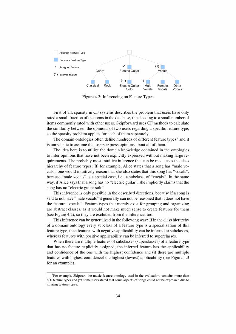
Figure 4.2: Inferencing on Feature Types

First of all, sparsity in CF systems describes the problem that users have onlyrated a small fraction of the items in the database, thus leading to a small number ofitems commonly rated with other users. Skipforward uses CF methods to calculatethe similarity between the opinions of two users regarding a specific feature type,so the sparsity problem applies for each of them separately.

The domain ontologies often define hundreds of different feature types5 and itis unrealistic to assume that users express opinions about all of them.

The idea here is to utilize the domain knowledge contained in the ontologiesto infer opinions that have not been explicitly expressed without making large re-quirements. The probably most intuitive inference that can be made uses the classhierarchy of feature types: If, for example, Alice states that a song has “male vo-cals”, one would intuitively reason that she also states that this song has “vocals”,because “male vocals” is a special case, i.e., a subclass, of “vocals”. In the sameway, if Alice says that a song has no “electric guitar”, she implicitly claims that thesong has no “electric guitar solo”.

This inference is only possible in the described directions, because if a song issaid to not have “male vocals” it generally can not be reasoned that it does not havethe feature “vocals”. Feature types that merely exist for grouping and organizingare abstract classes, as it would not make much sense to create features for them(see Figure 4.2), so they are excluded from the inference, too.

This inference can be generalized in the following way: If in the class hierarchyof a domain ontology every subclass of a feature type is a specialization of thisfeature type, then features with negative applicability can be inferred to subclasses,whereas features with positive applicability can be inferred to superclasses.

When there are multiple features of subclasses (superclasses) of a feature typethat has no feature explicitly assigned, the inferred feature has the applicabilityand confidence of the one with the highest confidence and (if there are multiplefeatures with highest confidence) the highest (lowest) applicability (see Figure 4.3for an example).

5For example, Skiptrax, the music feature ontology used in the evaluation, contains more than600 feature types and yet some users stated that some aspects of songs could not be expressed due tomissing feature types.

34

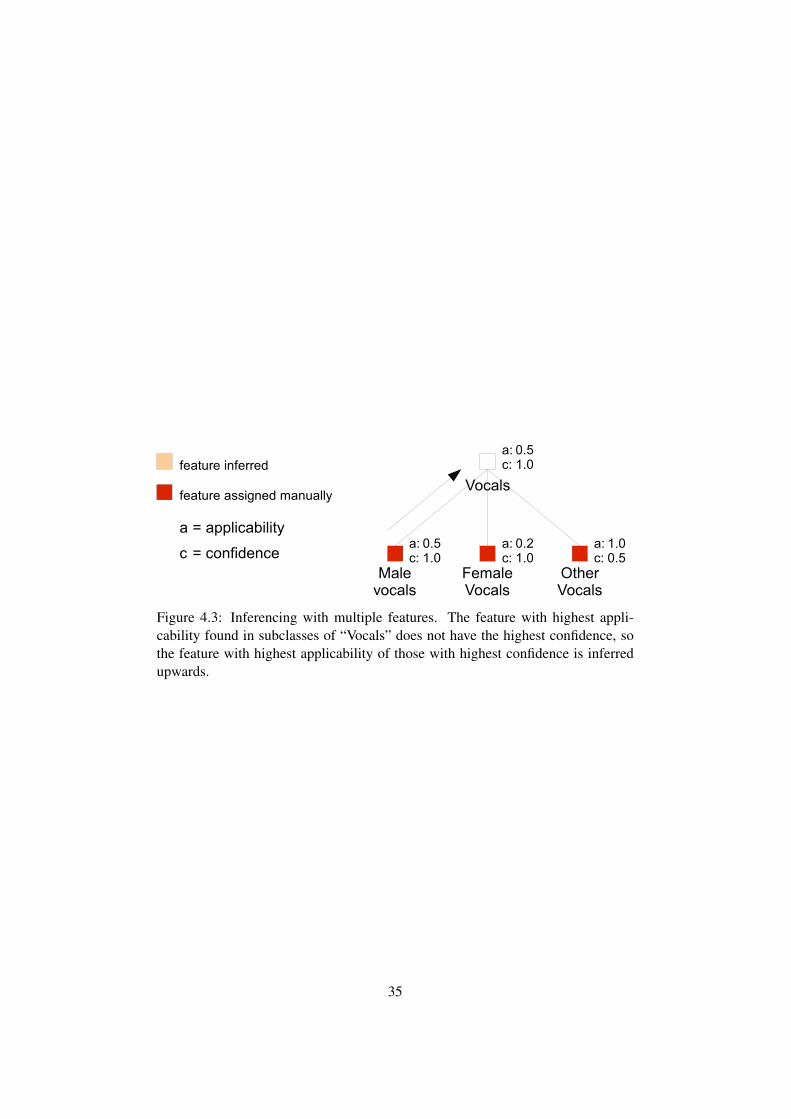
Figure 4.3: Inferencing with multiple features. The feature with highest appli-cability found in subclasses of “Vocals” does not have the highest confidence, sothe feature with highest applicability of those with highest confidence is inferredupwards.

35

Chapter 5

Implementation

When integrating the algorithms developed in this thesis into Skipforward, weadded it as an additional layer of functionality so that it is still possible to runSkipfoward without the new components. The data for the similarity calculationare stored separately from the items and their features, allowing a better abstractionfrom the data format and making it easier to develop and test the developed algo-rithms. The data repository of the SimilarityManager will be called cache fromhere on.

The traditional way of calculating the user similarities from scratch can easi-ly be accomplished by querying the Skipforward API for all items and their fea-tures, but in order to be able to incrementally update the similarities changes to thedatabase need to trigger the calculation somehow.

Changes to the database of a Skipforward node are made in two different ways:Firstly, by using the provided API through some user interface or other program,and secondly, through direct manipulation of the underlying RDF model by theSyncer component. Thus, it is not sufficient to modify the data changing methodsof the interface, but instead we have to listen to the RDF model directly to getnotified of changes.

The SimilarityManager, as we call the component that manages user similari-ties, listens for changes on the model and calculates the necessary updates when itdetects a change. Skipforward itself then can query those similarities and use themto personalize feature aggregations or compute recommendations.

5.1 Main algorithms

5.1.1 Initializing the similarity values

If a new user logs in into Skipforward for the first time, his database containsonly the Skipinions ontology and maybe some other domain ontologies. Startingwithout any features, all values that have to be cached for the incremental updateof the user similarities are 0 or undefined, so these values can be initialized lazily

36

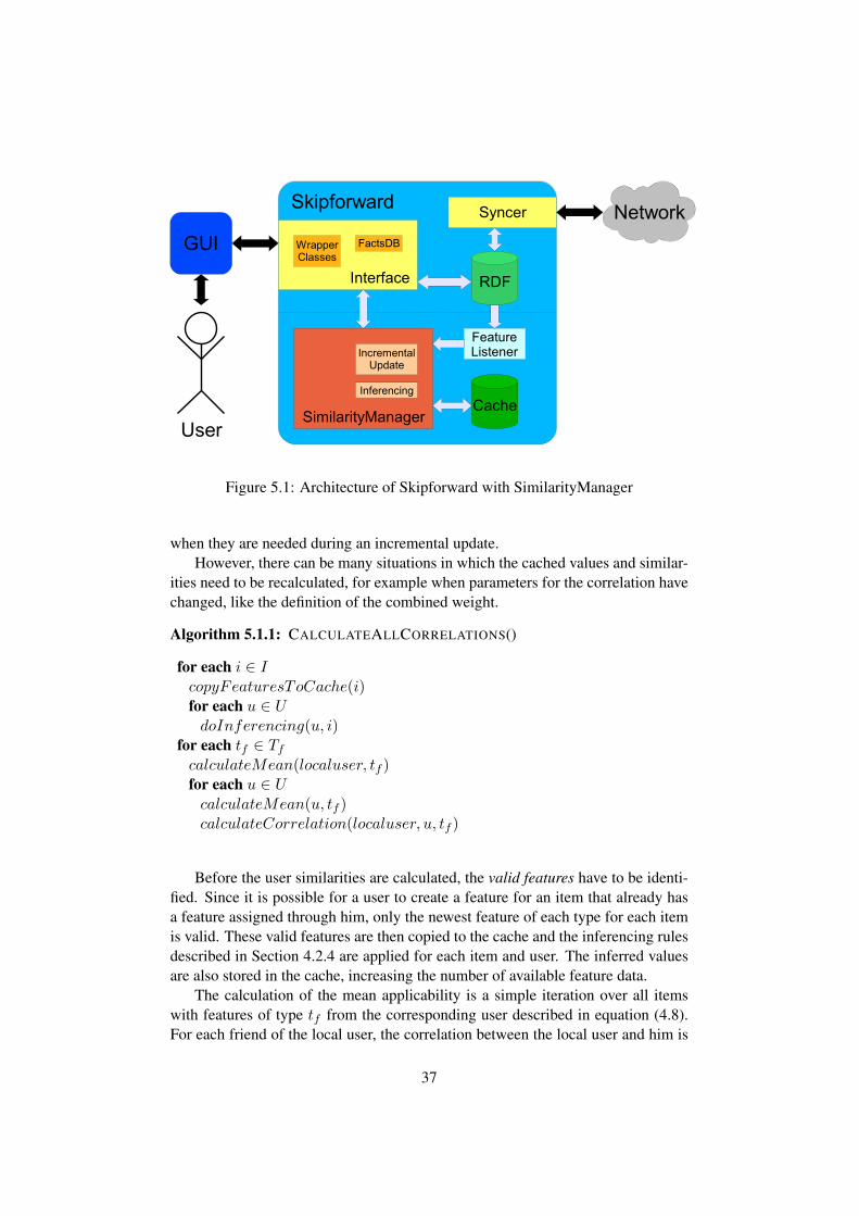
Figure 5.1: Architecture of Skipforward with SimilarityManager

when they are needed during an incremental update.However, there can be many situations in which the cached values and similar-

ities need to be recalculated, for example when parameters for the correlation havechanged, like the definition of the combined weight.

Algorithm 5.1.1: CALCULATEALLCORRELATIONS()

for each i ∈ IcopyFeaturesToCache(i)for each u ∈ UdoInferencing(u, i)

for each tf ∈ Tf

calculateMean(localuser, tf )for each u ∈ UcalculateMean(u, tf )calculateCorrelation(localuser, u, tf )

Before the user similarities are calculated, the valid features have to be identi-fied. Since it is possible for a user to create a feature for an item that already hasa feature assigned through him, only the newest feature of each type for each itemis valid. These valid features are then copied to the cache and the inferencing rulesdescribed in Section 4.2.4 are applied for each item and user. The inferred valuesare also stored in the cache, increasing the number of available feature data.

The calculation of the mean applicability is a simple iteration over all itemswith features of type tf from the corresponding user described in equation (4.8).For each friend of the local user, the correlation between the local user and him is

37

calculated according to equation (4.7), which essentially is an iteration of all itemsthat have features of type tf assigned by both users (explicitly or by inference).

During the calculation of the mean and the correlation, all values required bythe incremental update of user similarities can easily be obtained without a changein the computational complexity, since the number of iterations does not change.

5.1.2 Listening for feature changes

The FeatureListener is an implementation of the Jena ModelChangedListener in-terface that registers to the RDF model of Skipforward’s database and then getsnotified of every RDF statements that are added or removed from the model. Bythe time of notification, the changes to the model have already been made. For theupdate of user similarities, however, it is necessary to not only know the new validfeature values, but also the feature values that were valid before that.

For example, if a new feature was added, the notification of the FeatureLis-tener contains the information about this new feature, but none about if it made aprevious feature invalid and if it did, what applicability and confidence values theprevious one had. This information can be gathered by getting all features for thisitem (with the same feature type and from the same user) and looking for the onewith the latest creation date and that is not the one added.1

Although the necessary queries on the RDF model are not hard to implement,the performance heavily depends on the way the used RDF framework processesthese queries. Since every single feature change requires the lookup of the pre-viously valid feature values, this approach could easily increase the computationtime for similarity updates.

A faster solution to retrieve the old feature values is to get them from the cacheof the SimilaritiyManager. When initialized, the cache was filled with all validfeature values, the ones assigned by the user and the inferred ones. Hence, when theRDF model has been changed, the required information about its previous state canbe queried from the cache. However, after all user similarities have been updatedaccording to the feature changes, the feature values in the cache have to be updated,too.

5.1.3 Incremental update of similarity values

Every single feature change is handled separately and requires an update of one ormore user similarities, depending on who the changed feature belongs to. Sincewe only maintain the user similarities between the local user and his friends, onlyone update is necessary when the feature of another user has changed, but thesimilarities to all other users have to be updated if a feature of the local user haschanged (see Figure 5.2).

1As a real world example, imagine your bank sends you a notification and tells you that the newbalance of your account is 500 EUR. If you are interested in the difference to the previous balance(like we are here) you have to search for the latest balance notification before this new one.

38

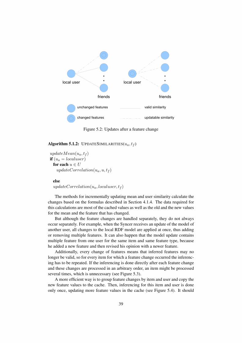
Figure 5.2: Updates after a feature change

Algorithm 5.1.2: UPDATESIMILARITIES(ua, tf )

updateMean(ua, tf )if (ua = localuser)

for each u ∈ UupdateCorrelation(ua, u, tf )

elseupdateCorrelation(ua, localuser, tf )

The methods for incrementally updating mean and user similarity calculate thechanges based on the formulas described in Section 4.1.4. The data required forthis calculations are most of the cached values as well as the old and the new valuesfor the mean and the feature that has changed.

But although the feature changes are handled separately, they do not alwaysoccur separately. For example, when the Syncer receives an update of the model ofanother user, all changes to the local RDF model are applied at once, thus addingor removing multiple features. It can also happen that the model update containsmultiple feature from one user for the same item and same feature type, becausehe added a new feature and then revised his opinion with a newer feature.

Additionally, every change of features means that inferred features may nolonger be valid, so for every item for which a feature change occurred the inferenc-ing has to be repeated. If the inferencing is done directly after each feature changeand these changes are processed in an arbitrary order, an item might be processedseveral times, which is unnecessary (see Figure 5.3).

A more efficient way is to group feature changes by item and user and copy thenew feature values to the cache. Then, inferencing for this item and user is doneonly once, updating more feature values in the cache (see Figure 5.4). It should

39

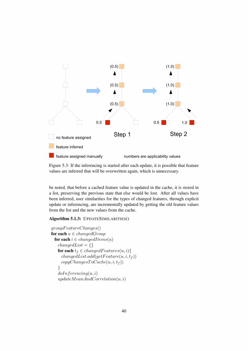
Figure 5.3: If the inferencing is started after each update, it is possible that featurevalues are inferred that will be overwritten again, which is unnecessary.

be noted, that before a cached feature value is updated in the cache, it is stored ina list, preserving the previous state that else would be lost. After all values havebeen inferred, user similarities for the types of changed features, through explicitupdate or inferencing, are incrementally updated by getting the old feature valuesfrom the list and the new values from the cache.

Algorithm 5.1.3: UPDATESIMILARITIES()

groupFeatureChanges()for each u ∈ changedGroup

for each i ∈ changedItems(u)changedList = {}for each tf ∈ changedFeatures(u, i){changedList.add(getFeature(u, i, tf ))copyChangesToCache(u, i, tf ))}doInferencing(u, i)updateMeanAndCorrelation(u, i)

40

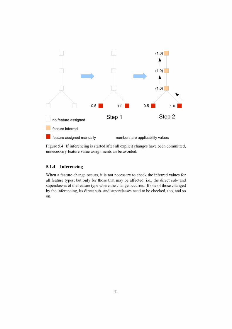
Figure 5.4: If inferencing is started after all explicit changes have been committed,unnecessary feature value assignments an be avoided.

5.1.4 Inferencing

When a feature change occurs, it is not necessary to check the inferred values forall feature types, but only for those that may be affected, i.e., the direct sub- andsuperclasses of the feature type where the change occurred. If one of those changedby the inferencing, its direct sub- and superclasses need to be checked, too, and soon.

41

Algorithm 5.1.4: UPDATESIMILARITIES()

updateSet = {}for each tf ∈ featureChangesupdateSet.addAll(tf .directSubClasses())updateSet.addAll(tf .directSuperClasses())

while not updateSet.isEmpty()

do

tf = updateSet.getF irstElement()updateSet.remove(tf )if tf .isAbstract() or tf .isExplicitlySet()

then continue

else

f = inferFeatureV alue(tf )if f 6= currentFeature(tf )

then

updateSet.addAll(tf .directSubClasses())updateSet.addAll(tf .directSuperClasses())setCurrentFeature(tf , f)

Essentially, everytime a feature is changed, the direct sub- and superclasses ofits feature type are added to a list of feature types that may need to be updated.Then, a feature type of this list is removed and if it is not abstract or explicitly set,a new feature value is inferred with the rules described in Section 4.2.4. If thisfeature value is different from the current one (if one exists), the new one is set andits sub- and superclasses are again added to the list. This is repeated until the list isempty.

5.2 Data structures

To be able to implement the approaches described in Chapter 4, different types ofdata need to be stored. The cache mainly contains two kinds of data: the validfeatures and the values necessary for incremental calculation of user similarities.

5.2.1 Feature Cache

As already mentioned in Section 5.1.2, caching the feature values can speed thingsup whenever the currently valid feature value needs to be queried, so the data struc-ture should be fast. On the other hand, the knowledge we have about the nature ofthe data should be used to reduce memory consumption.

What needs to be stored?

Since the calculation of user similarities is based on calculation done in collabo-rative filter, it is suggesting to base the data structure for the feature values on theuser-item matrices (see Section 3.2.1). The user-item matrix in CF stores the rat-ings users assign to items and the approach of this thesis is to view every single

42

Figure 5.5: User-Item-FeatureType Matrix

feature type as its own type of rating. Consequently, the feature values in Skip-forward can be represented by a 3-dimensional user-item-featuretype matrix (seeFigure 5.5).

There are many possibilities to represent a 3-dimensional matrix and each hasits pros and cons, so we need to examine the properties of the data that are to bestored.

Data sparsity The matrix will be mostly empty due to the sparsity of data. Asimple 3-dimensional array would not be suitable here, because the memoryneeded to store the array is allocated at its creation time, even if most of thecells in the matrix stay empty.

Access order Feature values may be accessed in different succession, such asitem-by-item during inferencing, or one feature type at a time when initial-izing user similarities, so the data structure has to be fast regardless of theorder in which elements are accessed.

Variable size The three dimensions have variable size, since users, items and fea-ture types can be added or removed from the database at any time

Element addressing Feature values are addressed by an URI for each dimension,not integer numbers. Additionally, the URIs for items differ from user touser, because they have to be in his namespace.

Sparse matrices and element addressing

In our implementation we use the Colt2 library, because it was developed to workwith large datasets with respect to performance and efficiency and provides a stablerelease. In particular, it offers implementations of sparse matrices, where cells thatare zero do not consume memory and access to cells has an expected complexity

2http://acs.lbl.gov/~hoschek/colt/

43

of O(1). Therefore, it fulfills our first two criteria, low memory consumption forsparse matrices and fast access time in any order.

The size of these matrices is fixed and has to be specified at creation time, sowe need to simply create the matrix as large as possible, since empty cells do notuse memory.

The biggest problem that has to be solved is the way in which cells are ad-dressed, because most matrix implementations only allow integer values for in-dices. The values that are used in Skipforward to uniquely address a valid featureare all complex objects, but they can be reduced to unique string representations:Each item or feature type can be uniquely identified by its URI, and each user canbe uniquely identified by his account name or namespace, which all are strings.

Strings can not be used as indices for the matrix, so we have to define a map-ping from strings to integer indices. This mapping can not be realized through ahash function, because the number of valid integers it very small compared to thenumber of possible URIs and it is not known in advance which URIs will be used.

Therefore, the mapping has to be established on-demand: If the integer valuerepresenting the index of a specific URI is requested but not defined, an unusedinteger value will be assigned to it and stored. The next time the index for this URIis queried, the previously assigned integer value will be returned.

Since the matrix and therefore its dimensions have fixed size, the availableinteger indices are limited and thus the number of users, items and feature typesthat can be addressed, too. If all available indices for items are already used, newitems can not be addressed and feature values for them can not be stored, even ifthere is plenty of space in the matrix.

The next problem related to URIs is the identity of items: As described inSection 2.4, every user describes only items in his own namespace and the transitiveisIdenticalTo relation is used to define that two resources of different namespacesactually refer to the same item. Consequently, each item may have multiple URIsreferring to it. So, either the mapping from URIs to integer values has to supportmultiple URIs mapping to the same value, or it has to be ensured that each itemis always identified by the same URI. We chose the second approach, becausemapping multiple URIs to one integer value would require us to keep track ofchanges in isIdenticalTo relations, which makes things more complicated and errorprone.

Instead of having one 3-dimensional user-item-featuretype matrix for every-thing, we create a separate 2-dimensional item-featuretype matrix and a separateitem-index mapping for each user. Since there are only feature values from oneuser stored in this matrix, all items this user has assigned features to have an URIin his namespace. Consequently, if there is no URI for an item in the user’s name-space, he has not assigned any features to it and there are no values to be stored inthis matrix.

Additionally, the memory is used more efficiently, because each matrix con-tains only rows for the items its user has assigned features to and the item-indexmapping maps only URIs of the user’s namespace.

44

However, when querying items that have been co-rated, i.e., two users haveassigned features of the same type to it, this is not evident from the matrix and themapping alone. For each user, the items with features of this type in his name-space have to be retrieved and the semantically identical ones have to be found byquerying the RDF store.

5.2.2 Incremental user similarities

The incremental calculation of user similarities requires the caching of values foreach feature type and for each user and each pair of users for which a similarityshould be calculated. Examples for user-specific values are the mean applicabilityand the sum of confidence values of features of type tf , whereas the factors B, Cand D have to be stored for each pair of users (see Section 4.1.4 for a completelist).

These values can be stored in hash maps or other simple data objects. To in-crease memory efficiency, these data objects are instantiated lazily, because thevalues for many feature types are often 0 if there are no co-rated items with otherusers. Instead of storing these “empty” values in an object, no object is created,which is interpreted by the system as “all values are 0”.

45

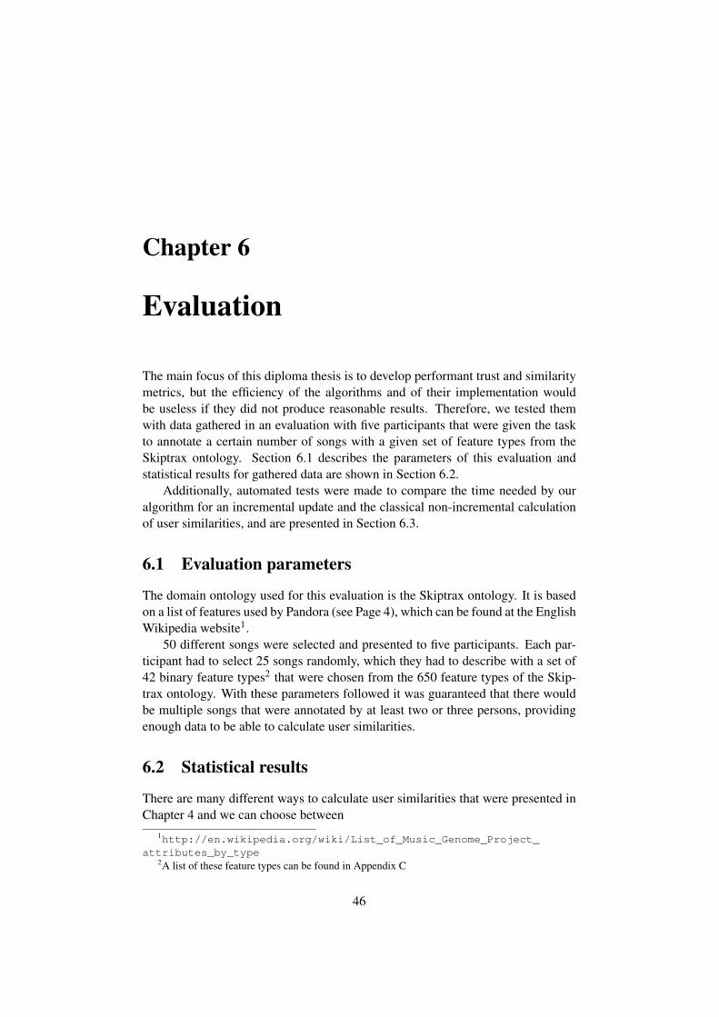
Chapter 6

Evaluation

The main focus of this diploma thesis is to develop performant trust and similaritymetrics, but the efficiency of the algorithms and of their implementation wouldbe useless if they did not produce reasonable results. Therefore, we tested themwith data gathered in an evaluation with five participants that were given the taskto annotate a certain number of songs with a given set of feature types from theSkiptrax ontology. Section 6.1 describes the parameters of this evaluation andstatistical results for gathered data are shown in Section 6.2.

Additionally, automated tests were made to compare the time needed by ouralgorithm for an incremental update and the classical non-incremental calculationof user similarities, and are presented in Section 6.3.

6.1 Evaluation parameters

The domain ontology used for this evaluation is the Skiptrax ontology. It is basedon a list of features used by Pandora (see Page 4), which can be found at the EnglishWikipedia website1.

50 different songs were selected and presented to five participants. Each par-ticipant had to select 25 songs randomly, which they had to describe with a set of42 binary feature types2 that were chosen from the 650 feature types of the Skip-trax ontology. With these parameters followed it was guaranteed that there wouldbe multiple songs that were annotated by at least two or three persons, providingenough data to be able to calculate user similarities.

6.2 Statistical results

There are many different ways to calculate user similarities that were presented inChapter 4 and we can choose between

1http://en.wikipedia.org/wiki/List_of_Music_Genome_Project_attributes_by_type

2A list of these feature types can be found in Appendix C

46

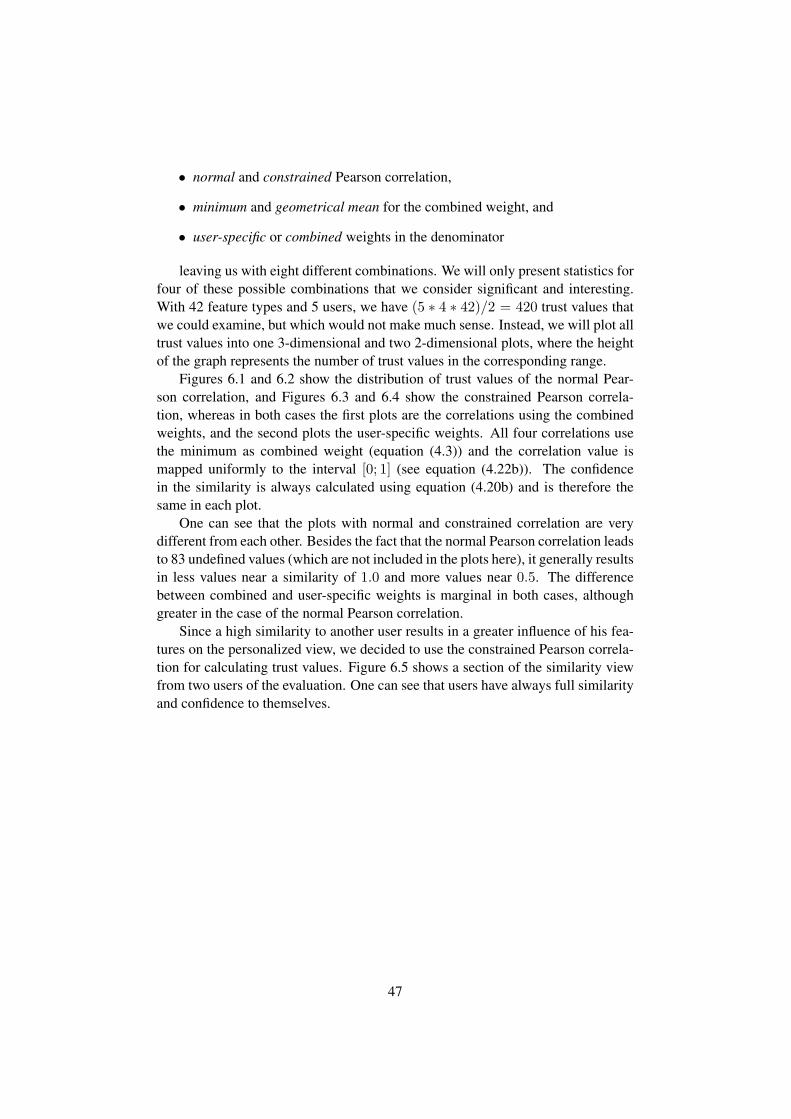
• normal and constrained Pearson correlation,

• minimum and geometrical mean for the combined weight, and

• user-specific or combined weights in the denominator

leaving us with eight different combinations. We will only present statistics forfour of these possible combinations that we consider significant and interesting.With 42 feature types and 5 users, we have (5 ∗ 4 ∗ 42)/2 = 420 trust values thatwe could examine, but which would not make much sense. Instead, we will plot alltrust values into one 3-dimensional and two 2-dimensional plots, where the heightof the graph represents the number of trust values in the corresponding range.

Figures 6.1 and 6.2 show the distribution of trust values of the normal Pear-son correlation, and Figures 6.3 and 6.4 show the constrained Pearson correla-tion, whereas in both cases the first plots are the correlations using the combinedweights, and the second plots the user-specific weights. All four correlations usethe minimum as combined weight (equation (4.3)) and the correlation value ismapped uniformly to the interval [0; 1] (see equation (4.22b)). The confidencein the similarity is always calculated using equation (4.20b) and is therefore thesame in each plot.

One can see that the plots with normal and constrained correlation are verydifferent from each other. Besides the fact that the normal Pearson correlation leadsto 83 undefined values (which are not included in the plots here), it generally resultsin less values near a similarity of 1.0 and more values near 0.5. The differencebetween combined and user-specific weights is marginal in both cases, althoughgreater in the case of the normal Pearson correlation.

Since a high similarity to another user results in a greater influence of his fea-tures on the personalized view, we decided to use the constrained Pearson correla-tion for calculating trust values. Figure 6.5 shows a section of the similarity viewfrom two users of the evaluation. One can see that users have always full similarityand confidence to themselves.

47

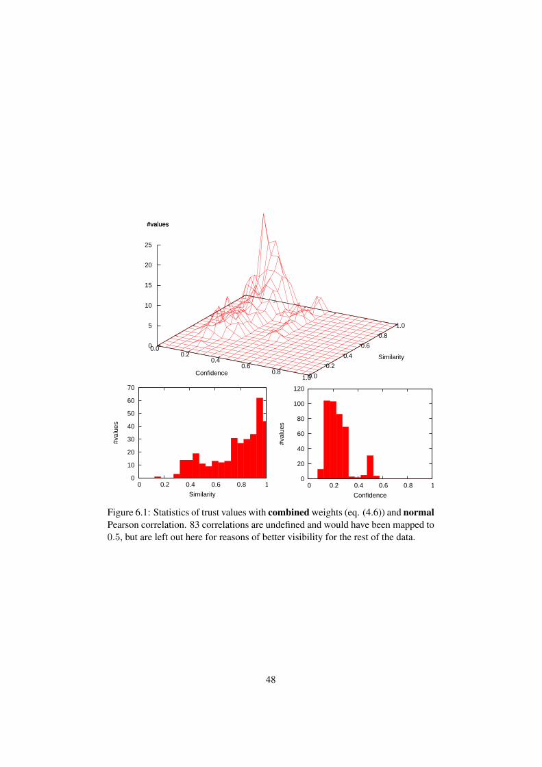
0.00.2

0.40.6

0.81.00.0

0.2

0.4

0.6

0.8

1.0

0

5

10

15

20

25

#values

Confidence

Similarity

#values

0

10

20

30

40

50

60

70

0 0.2 0.4 0.6 0.8 1

#val

ues

Similarity

0

20

40

60

80

100

120

0 0.2 0.4 0.6 0.8 1

#val

ues

Confidence

Figure 6.1: Statistics of trust values with combined weights (eq. (4.6)) and normalPearson correlation. 83 correlations are undefined and would have been mapped to0.5, but are left out here for reasons of better visibility for the rest of the data.

48

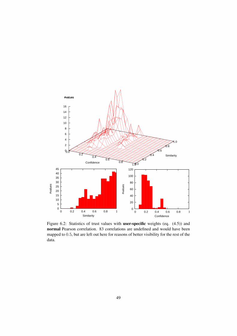
0.00.2

0.40.6

0.81.00.0

0.2

0.4

0.6

0.8

1.0

0

2

4

6

8

10

12

14

16

#values

Confidence

Similarity

#values

0

5

10

15

20

25

30

35

40

45

0 0.2 0.4 0.6 0.8 1

#val

ues

Similarity

0

20

40

60

80

100

120

0 0.2 0.4 0.6 0.8 1

#val

ues

Confidence

Figure 6.2: Statistics of trust values with user-specific weights (eq. (4.5)) andnormal Pearson correlation. 83 correlations are undefined and would have beenmapped to 0.5, but are left out here for reasons of better visibility for the rest of thedata.

49

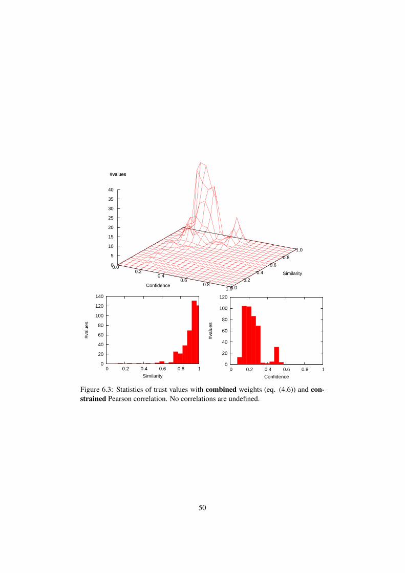
0.00.2

0.40.6

0.81.00.0

0.2

0.4

0.6

0.8

1.0

0

5

10

15

20

25

30

35

40

#values

Confidence

Similarity

#values

0

20

40

60

80

100

120

140

0 0.2 0.4 0.6 0.8 1

#val

ues

Similarity

0

20

40

60

80

100

120

0 0.2 0.4 0.6 0.8 1

#val

ues

Confidence

Figure 6.3: Statistics of trust values with combined weights (eq. (4.6)) and con-strained Pearson correlation. No correlations are undefined.

50

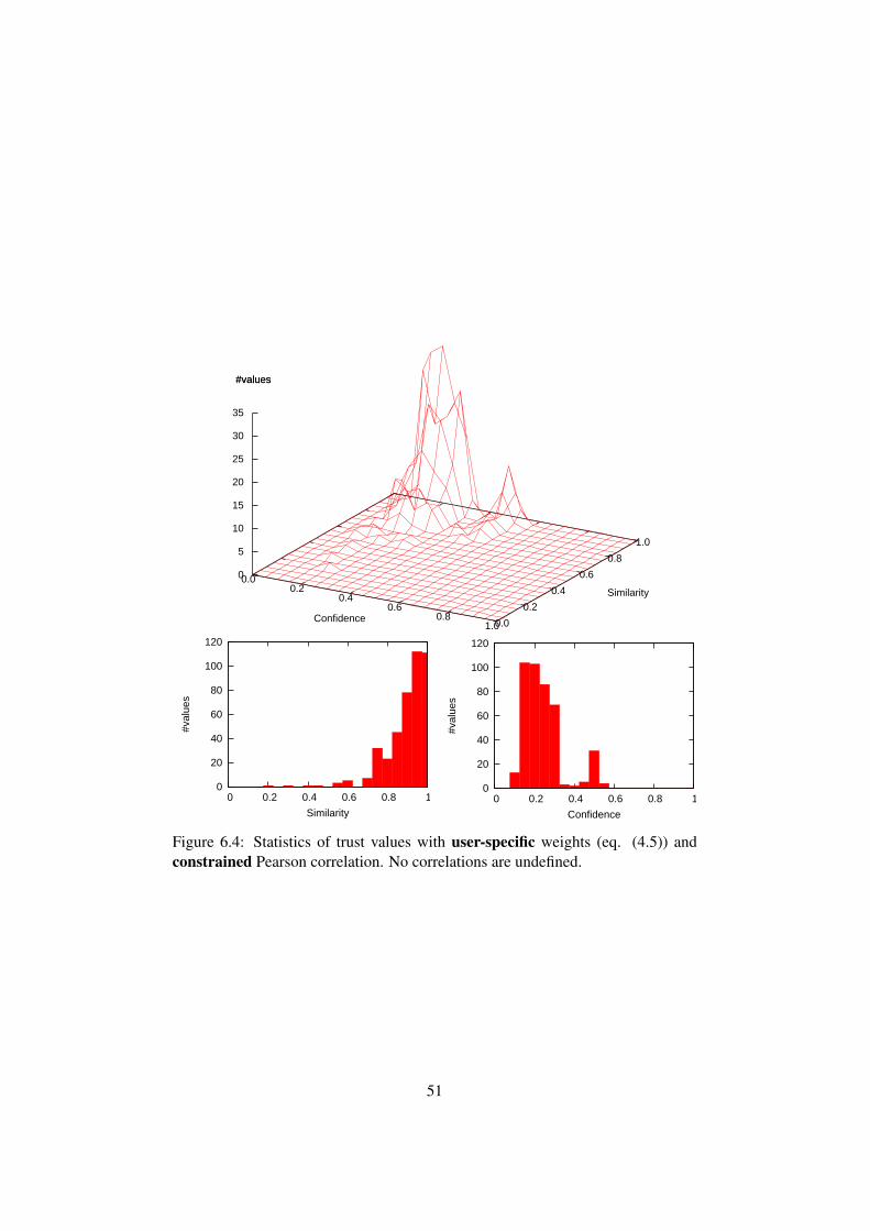
0.00.2

0.40.6

0.81.00.0

0.2

0.4

0.6

0.8

1.0

0

5

10

15

20

25

30

35

#values

Confidence

Similarity

#values

0

20

40

60

80

100

120

0 0.2 0.4 0.6 0.8 1

#val

ues

Similarity

0

20

40

60

80

100

120

0 0.2 0.4 0.6 0.8 1

#val

ues

Confidence

Figure 6.4: Statistics of trust values with user-specific weights (eq. (4.5)) andconstrained Pearson correlation. No correlations are undefined.

51

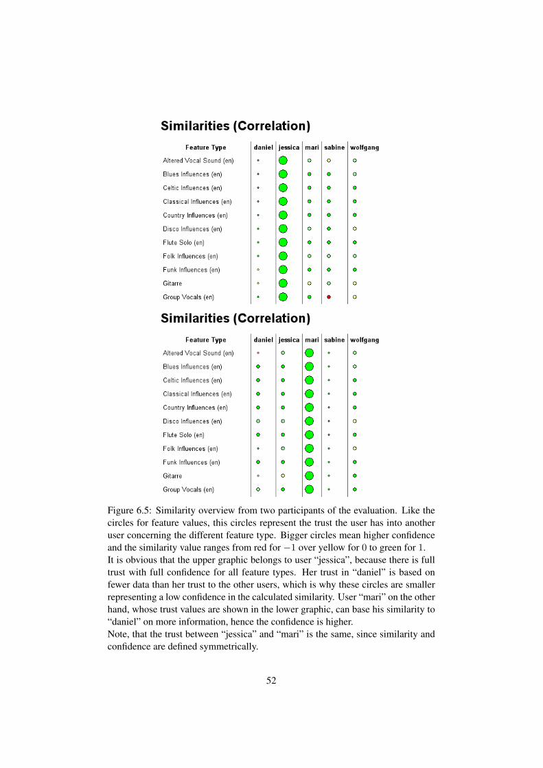
Figure 6.5: Similarity overview from two participants of the evaluation. Like thecircles for feature values, this circles represent the trust the user has into anotheruser concerning the different feature type. Bigger circles mean higher confidenceand the similarity value ranges from red for −1 over yellow for 0 to green for 1.It is obvious that the upper graphic belongs to user “jessica”, because there is fulltrust with full confidence for all feature types. Her trust in “daniel” is based onfewer data than her trust to the other users, which is why these circles are smallerrepresenting a low confidence in the calculated similarity. User “mari” on the otherhand, whose trust values are shown in the lower graphic, can base his similarity to“daniel” on more information, hence the confidence is higher.Note, that the trust between “jessica” and “mari” is the same, since similarity andconfidence are defined symmetrically.

52

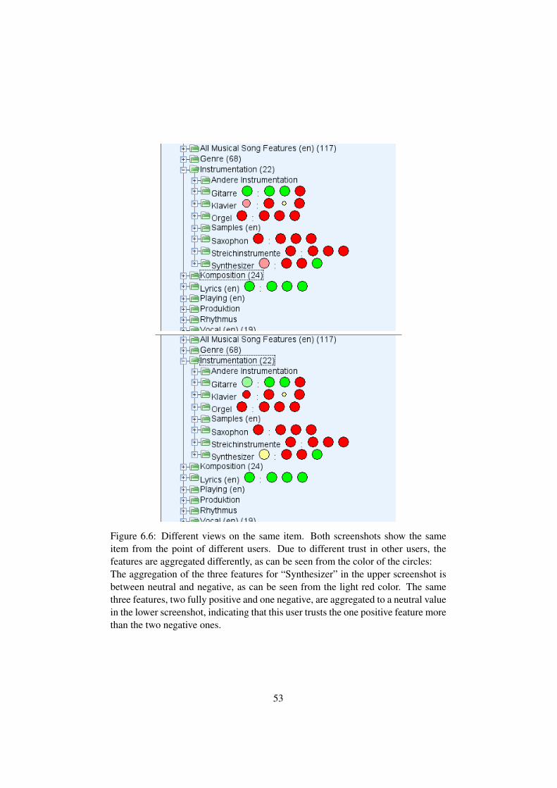
Figure 6.6: Different views on the same item. Both screenshots show the sameitem from the point of different users. Due to different trust in other users, thefeatures are aggregated differently, as can be seen from the color of the circles:The aggregation of the three features for “Synthesizer” in the upper screenshot isbetween neutral and negative, as can be seen from the light red color. The samethree features, two fully positive and one negative, are aggregated to a neutral valuein the lower screenshot, indicating that this user trusts the one positive feature morethan the two negative ones.

53

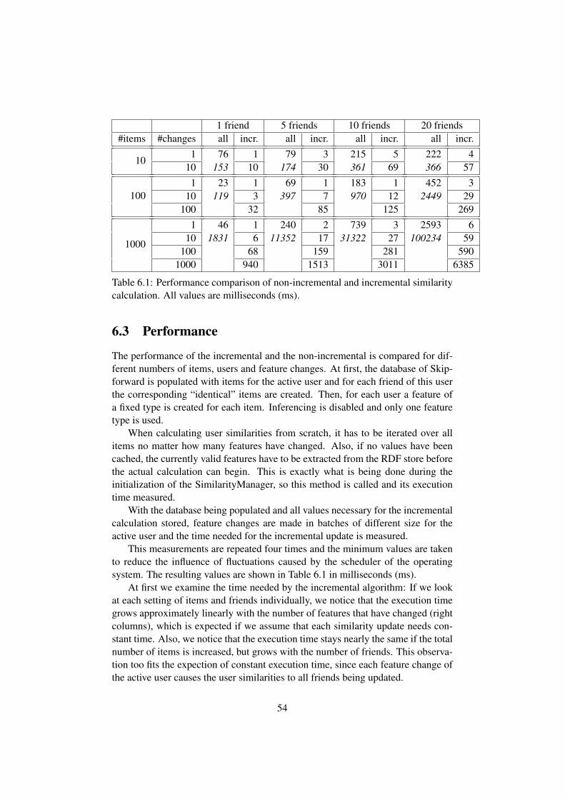
1 friend 5 friends 10 friends 20 friends#items #changes all incr. all incr. all incr. all incr.

101 76 1 79 3 215 5 222 4

10 153 10 174 30 361 69 366 57

1001 23 1 69 1 183 1 452 3

10 119 3 397 7 970 12 2449 29100 32 85 125 269

1000

1 46 1 240 2 739 3 2593 610 1831 6 11352 17 31322 27 100234 59

100 68 159 281 5901000 940 1513 3011 6385

Table 6.1: Performance comparison of non-incremental and incremental similaritycalculation. All values are milliseconds (ms).

6.3 Performance

The performance of the incremental and the non-incremental is compared for dif-ferent numbers of items, users and feature changes. At first, the database of Skip-forward is populated with items for the active user and for each friend of this userthe corresponding “identical” items are created. Then, for each user a feature ofa fixed type is created for each item. Inferencing is disabled and only one featuretype is used.

When calculating user similarities from scratch, it has to be iterated over allitems no matter how many features have changed. Also, if no values have beencached, the currently valid features have to be extracted from the RDF store beforethe actual calculation can begin. This is exactly what is being done during theinitialization of the SimilarityManager, so this method is called and its executiontime measured.

With the database being populated and all values necessary for the incrementalcalculation stored, feature changes are made in batches of different size for theactive user and the time needed for the incremental update is measured.

This measurements are repeated four times and the minimum values are takento reduce the influence of fluctuations caused by the scheduler of the operatingsystem. The resulting values are shown in Table 6.1 in milliseconds (ms).

At first we examine the time needed by the incremental algorithm: If we lookat each setting of items and friends individually, we notice that the execution timegrows approximately linearly with the number of features that have changed (rightcolumns), which is expected if we assume that each similarity update needs con-stant time. Also, we notice that the execution time stays nearly the same if the totalnumber of items is increased, but grows with the number of friends. This observa-tion too fits the expection of constant execution time, since each feature change ofthe active user causes the user similarities to all friends being updated.

54

The time needed by the non-incremental algorithm is shown in the leftcolumns, the values in normal letters are the times for calculation only, whereasthe italic values are the times needed for complete initialization process. Thesevalues have a higher fluctuation than those of the incremental updates, but theygenerally tend to grow with the number of items and friends.

One may notice that the execution time of the initialization method does notincrease linearly but stronger. A possible reason for this becomes apparent whenlooking closer at the process of populating the RDF database. As it turns out, thetime needed to add items and features to the database increases with the size of thedatabase. If the access time of the RDF store is not constant, this might slow downthe calculation of the user similarities as well.

It should also be mentioned, that with an increasing number of total items, theincremental update becomes less performant for larger feature changes comparedto the non-incremental calculation. This is not suprising, since the equations forthe incremental update are rather complex and when a certain amount of featurechanges is exceeded, it is more performant to do a non-incremental calculation ofthe similarity values.

55

Chapter 7

Summary and Outlook

In this thesis, we have developed incremental algorithms to calculate similaritiesbetween users based on opinions they have expressed. We were able to use thesesimilarities as trust values to create a personalized view on a knowledge-base thatis inherently inconsistent. These personalized views provide a useful foundationto build mechanisms upon it that help the user in his task of identifying relevantinformation in large data sets.

The algorithms are based on well established methods in the field of Recom-mender Systems and combine aspects of both collaborative and content-based fil-tering. The incremental calculation of user similarities during the usage of Skip-forward ensures that the data necessary for the aggregation of features and recom-mendation of interesting items is always updated and at hand.

We evaluated the results of our algorithms on the basis of annotations of mu-sic of five persons collected in a test period of three weeks and the gathered datawas sufficient to indicate the plausibility of the results. Nevertheless, an extendedsurvey with more participants should be performed to verify the quality of the per-sonalization of data.

Experiments regarding the performance of the incremental algorithms haveshown that they are indeed faster than the classical non-incremental calculationof similarities for many cases. Also, the absolute time needed for the incrementalupdates on an ordinary computer is in the region of seconds, making it practicablefor use on personal computers.

7.1 Outlook

7.1.1 Optimization of data structures

For the implementation of our algorithms we used the Jena and the Colt frameworkfor storage, because it allowed us to concentrate on the main tasks of this thesis.However, during the implementation we encountered some complications becauseof the different ways in which data is addressed. The mapping from URIs to integer

56

values as indices and vice-versa does not only consume memory, but it also takessome time to do the mapping.

Instead of translating between both frameworks, it should be investigated ifmore efficient ways for storing the data required for our algorithms can be devel-oped.

7.1.2 Relationships between feature types

Currently, the only relationship between feature types that is used in the calcula-tions is the subtype relationship. This allows us to infer some features that theuser implicitly defined by explicitly assigning another feature. The feature typehierarchy is defined in the domain ontologies and the creator of the ontology isresponsible for designing these relationships properly.

There may be dependencies between different feature types that where not ap-parent to the ontology creator or that are not generally valid for all users. Differenttechniques for discovering these relationships are possible. For example, the al-ready used correlation coefficient could be used to examine dependencies betweenfeature types. This or other approaches might be suitable to further increase theinformation that can be automatically extracted from the user’s inputs.

7.1.3 Handling of non-binary feature types

The user similarities used in this thesis were based on binary feature types only,reducing the complexity of possible similarity functions. However, valuable infor-mation is ignored when non-binary features are not included in this similarities.

To some extent, non-binary feature types are replacements for a whole set ofbinary feature types. For example, instead of having dozens of different binaryfeature types for different kinds of musical influences, e.g., “Disco influences”,“Jazz influences”, “Rap influences”, there could be only one non-binary featuretype “hasInfluence” whose feature instances point to objects or items representingdifferent influences.

In fact, this is sometimes the only possibility to represent certain features, be-cause the number of available objects is infinite or unknown. For example, in-stead of using the feature type “MainArtist” that points to an item of type Artist,it would be possible to create an extra feature type for every artist available, like“MainArtist is Madonna”, “MainArtist is Tina Turner”, etc. However, this wouldmassively increase the number of feature types for the same amount of informationand therefore the sparsity of the data would also be increased.

There are some aspects regarding non-binary features that have to be furtherexamined:

57

Similarity of objects

If two users have assigned a feature of the same type to the same item, but thefeature have different object, e.g. “MainArtist” with different artists, what is thesimilarity between these features? It could be as trivial as defining the similarity tobe 1 if the objects are identical and 0 else. But depending on the type of the object,there could be a special similarity metric defined for it, e.g., the Hamming-distancefor strings.

In either case, the algorithms developed in this thesis can not be applied to non-binary features without modification and the data structures used are not suitablein their current form, either.

Similarities on non-binary feature types

The easiest way to define user similarities on non-binary feature types would beto have a separate similarity for each combination of feature type and object. Forexample, if two users agree that “Madonna” is an artist of a certain song, but dis-agree whether “Britney Spears” is an artist of this song, too, they would have ahigh similarity on opinions regarding Madonna being the artist of a song and a lowsimilarity for Britney Spears. But it is not intuitively clear what is their similarityon the feature type “Artist” in general.

Further work is needed to define plausible rules and algorithms that processthis information in a useful way.

7.1.4 Similarities on partial data sets

As already mentioned in Section 1.1, users can have different opinions on a certaintopic while agreeing on another. Because user similarities are calculated separatelyfor each feature type, a low similarity on one feature type does not influence thesimilarity of opinions of another type, allowing a very differentiated view of thecompetence of another user. This, however, is only because most feature type arerestricted to a specific domain, e.g., “Strong melody”.

When a feature type can be applied to a wide range of item types, a differen-tiation of user similarities can not easily be accomplished. A good example forthis problem is the feature type skipinions:Review, which is used to express onesliking of an item and can be applied to items of different types. However, for eachpair of users only one value for the similarity on this feature type is calculated.This means that if two users have the same taste regarding music but enjoy totallydifferent movies, the calculation will not distinguish between those item types andresult in an intermediate similarity value.

58

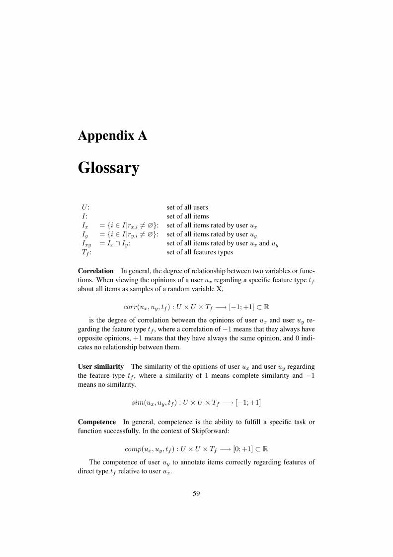
Appendix A

Glossary

U : set of all usersI: set of all itemsIx = {i ∈ I|rx,i 6= ∅}: set of all items rated by user ux

Iy = {i ∈ I|ry,i 6= ∅}: set of all items rated by user uy

Ixy = Ix ∩ Iy: set of all items rated by user ux and uy

Tf : set of all features types

Correlation In general, the degree of relationship between two variables or func-tions. When viewing the opinions of a user ux regarding a specific feature type tfabout all items as samples of a random variable X,

corr(ux, uy, tf ) : U × U × Tf −→ [−1; +1] ⊂ R

is the degree of correlation between the opinions of user ux and user uy re-garding the feature type tf , where a correlation of −1 means that they always haveopposite opinions, +1 means that they have always the same opinion, and 0 indi-cates no relationship between them.

User similarity The similarity of the opinions of user ux and user uy regardingthe feature type tf , where a similarity of 1 means complete similarity and −1means no similarity.

sim(ux, uy, tf ) : U × U × Tf −→ [−1; +1]

Competence In general, competence is the ability to fulfill a specific task orfunction successfully. In the context of Skipforward:

comp(ux, uy, tf ) : U × U × Tf −→ [0; +1] ⊂ R

The competence of user uy to annotate items correctly regarding features ofdirect type tf relative to user ux.

59

Expert A user with a high competence in some domain. Due to the relativenessof competence, the role of an expert is also defined relative to another user. Userux calls user uy an expert, if

comp(ux, uy, tf ) ≥ threshux

where threshux ∈ [0; +1] is a threshold defined by user ux.

Neighbor The term neighbor is used in the context of collaborative filtering anddescribes users that have similar taste. It is a special case of an expert, where thefeature type tf is some kind of rating and, therefore, similarity and competencerelate to the users taste.

60

Appendix B

Proof of equations

Note: I ′xy is the set of co-rated items without the active item (the one for which thefeature change appeared).

B′ =∑i∈Ixy

w′xy,i(xi − x′)(yi − y)

= w′xy,i(x′a − x′)(ya − y) +

∑i∈I′

xy

wxy,i(xi − x′)(yi − y)

= (wxy,a + dwxy,a)(xa + dxa − x′)(ya − y) +∑i∈I′

xy

wxy,i(xi − x′)(yi − y)

= (wxy,a + dwxy,a)(dxa(ya − y) + (xa − x′)(ya − y)

+∑i∈I′

xy

wxy,i(xi − x′)(yi − y)

= dwxy,a(xa + dxa − x′)(ya − y) + wxy,adxa(ya − y) + wxy,a(xa − x′)(ya − y)

+∑i∈I′

xy

wxy,i(xi − x′)(yi − y)

= dwxy,a(xa + dxa − x′)(ya − y) + wxy,adxa(ya − y) +∑i∈Ixy

wxy,i(xi − x′)(yi − y)

= dwxy,a(xa + dxa − x′)(ya − y) + wxy,adxa(ya − y) +B − dx(∑i∈Ixy

(wxy,iyi)− y∑i∈Ixy

wxy,i)

61

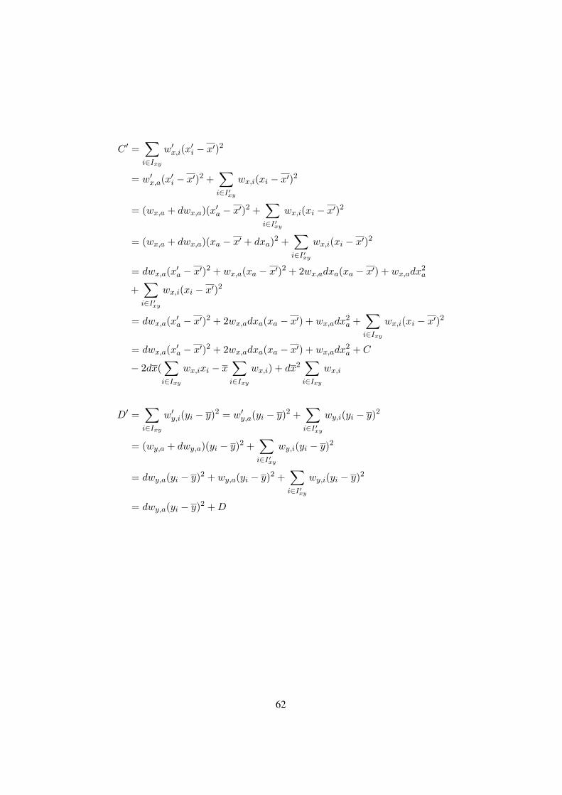
C ′ =∑i∈Ixy

w′x,i(x′i − x′)2

= w′x,a(x′i − x′)2 +∑i∈I′

xy

wx,i(xi − x′)2

= (wx,a + dwx,a)(x′a − x′)2 +∑i∈I′

xy

wx,i(xi − x′)2

= (wx,a + dwx,a)(xa − x′ + dxa)2 +∑i∈I′

xy

wx,i(xi − x′)2

= dwx,a(x′a − x′)2 + wx,a(xa − x′)2 + 2wx,adxa(xa − x′) + wx,adx2a

+∑i∈I′

xy

wx,i(xi − x′)2

= dwx,a(x′a − x′)2 + 2wx,adxa(xa − x′) + wx,adx2a +

∑i∈Ixy

wx,i(xi − x′)2

= dwx,a(x′a − x′)2 + 2wx,adxa(xa − x′) + wx,adx2a + C

− 2dx(∑i∈Ixy

wx,ixi − x∑i∈Ixy

wx,i) + dx2∑i∈Ixy

wx,i

D′ =∑i∈Ixy

w′y,i(yi − y)2 = w′y,a(yi − y)2 +∑i∈I′

xy

wy,i(yi − y)2

= (wy,a + dwy,a)(yi − y)2 +∑i∈I′

xy

wy,i(yi − y)2

= dwy,a(yi − y)2 + wy,a(yi − y)2 +∑i∈I′

xy

wy,i(yi − y)2

= dwy,a(yi − y)2 +D

62

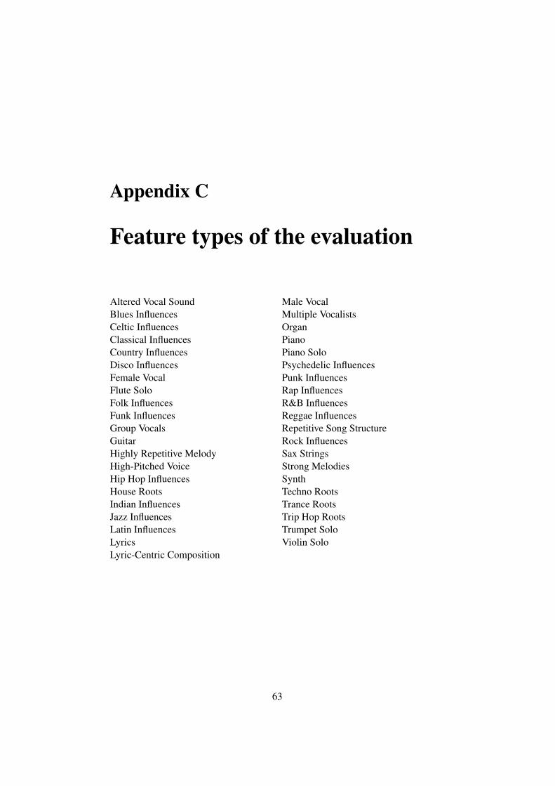
Appendix C

Feature types of the evaluation

Altered Vocal SoundBlues InfluencesCeltic InfluencesClassical InfluencesCountry InfluencesDisco InfluencesFemale VocalFlute SoloFolk InfluencesFunk InfluencesGroup VocalsGuitarHighly Repetitive MelodyHigh-Pitched VoiceHip Hop InfluencesHouse RootsIndian InfluencesJazz InfluencesLatin InfluencesLyricsLyric-Centric Composition

Male VocalMultiple VocalistsOrganPianoPiano SoloPsychedelic InfluencesPunk InfluencesRap InfluencesR&B InfluencesReggae InfluencesRepetitive Song StructureRock InfluencesSax StringsStrong MelodiesSynthTechno RootsTrance RootsTrip Hop RootsTrumpet SoloViolin Solo

63

Bibliography

Adams, B. D. (2005). Trust vs. confidence. Technical report, Defence Researchand Development Canada.

Adomavicius, G. and Tuzhilin, A. (2005). Toward the next generation of rec-ommender systems: A survey of the state-of-the-art and possible extensions.IEEE Transactions on Knowledge and Data Engineering, 17(6):734–749.

Anscombe, F. J. (1973). Graphs in statistical analysis. The American Statistician,27(1):17–21.

Balabanovic, M. and Shoham, Y. (1997). Fab: content-based, collaborative recom-mendation. Communications of the ACM, 40(3):66–72.

Carroll, J. (1961). The nature of the data, or how to choose a correlation coefficient.Psychometrika, 26(4):347–372.

Gutscher, A., Heesen, J., and Siemoneit, O. (2008). Possibilities and limitations ofmodeling trust and reputation. In Möller, M., Roth-Berghofer, T., and Neuser,W., editors, WSPI, volume 332 of CEUR Workshop Proceedings, pages 50–61. CEUR-WS.org.

Jøsang, A., Ismail, R., and Boyd, C. (2007). A survey of trust and reputationsystems for online service provision. Decision Support Systems, 43(2):618–644.

Kiesel, M. and Schwarz, S. (2008). Skipforward - a lightweight ontology-basedpeer-to-peer recommendation system. In Bizer, C. and Joshi, A., editors,International Semantic Web Conference (Posters & Demos), volume 401 ofCEUR Workshop Proceedings. CEUR-WS.org.

Linden, G., Smith, B., and York, J. (2003). Amazon. com recommendations: Item-to-item collaborative filtering. IEEE Internet Computing, pages 76–80.

Liu, Z., Wang, Y., and Chen, T. (1998). Audio feature extraction and analysis forscene segmentation and classification. The Journal of VLSI Signal Processing,20(1):61–79.

64

Marsh, S. P., of Computing Science, D., Mathematics, and of Stirling, U. (1995).Formalising Trust as a Computational Concept. Dept. of Computing Scienceand Mathematics, University of Stirling.

Massa, P. and Avesani, P. (2004). Trust-aware collaborative filtering for recom-mender systems. Lecture Notes in Computer Science, pages 492–508.

Massa, P. and Bhattacharjee, B. (2004). Using trust in recommender systems: Anexperimental analysis. Lecture Notes in Computer Science, pages 221–235.

Maurer, U. (1996). Modelling a public-key infrastructure. Lecture Notes in Com-puter Science, pages 325–350.

O’Donovan, J. and Smyth, B. (2005). Trust in recommender systems.

O’Mahony, M. P., Hurley, N. J., and Silvestre, G. C. M. (2002). Promoting rec-ommendations: An attack on collaborative filtering. In Proceedings of the13th International Conference on Database and Expert Systems Applications(DEXA), 2nd–6th, volume LNCS 2453, pages 494–503, Aix-en-Provence,France. Springer-Verlag.

Papagelis, M., Rousidis, I., Plexousakis, D., and Theoharopoulos, E. (2005). Incre-mental collaborative filtering for highly-scalable recommendation algorithms.In Hacid, M.-S., Murray, N. V., Ras, Z. W., and Tsumoto, S., editors, ISMIS,volume 3488 of Lecture Notes in Computer Science, pages 553–561. Springer.

Pazzani, M. (1999). A framework for collaborative, content-based and demo-graphic filtering. Artificial Intelligence Review, 13(5):393–408.

Rodgers, J. L. and Nicewander, A. W. (1988). Thirteen ways to look at the corre-lation coefficient. The American Statistician, 42(1):59–66.

Sarwar, B., Karypis, G., Konstan, J., and Reidl, J. (2001). Item-based collaborativefiltering recommendation algorithms. In WWW ’01: Proceedings of the 10thinternational conference on World Wide Web, pages 285–295, New York, NY,USA. ACM.

Sarwar, B., Karypis, G., Konstan, J., Riedl, J., and SCIENCE, M. U. M. D. O. C.(2000). Application of Dimensionality Reduction in Recommender System-ACase Study. Defense Technical Information Center.

Schafer, J. B., Konstan, J., and Riedi, J. (1999). Recommender systems in e-commerce. In EC ’99: Proceedings of the 1st ACM conference on Electroniccommerce, pages 158–166, New York, NY, USA. ACM.

Shafer, G. (1976). A mathematical theory of evidence. Princeton University PressPrinceton, NJ.

65

Shardanand, U. and Maes, P. (1995). Social information filtering: algorithms forautomating "word of mouth". In CHI ’95: Proceedings of the SIGCHI con-ference on Human factors in computing systems, pages 210–217, New York,NY, USA. ACM Press/Addison-Wesley Publishing Co.

Wang, Y. and Vassileva, J. (2003). Trust and reputation model in peer-to-peernetworks. Peer-to-Peer Computing, IEEE International Conference on, pages150–157.

Ziegler, C. and Lausen, G. (2004). Analyzing correlation between trust and usersimilarity in online communities. Lecture Notes in Computer Science, pages251–265.

66