Czech Technical University in Prague

Faculty of Electrical Engineering

DIPLOMA THESIS

Bc. Jirı Valtr

Mass Flow Estimation and Control in PumpDriven Hydronic Systems

Department of Cybernetics

Supervisor: Ing. Jirı Dostal

Prague, January 2017

Author Statement

I declare that the presented work was developed independently and that I havelisted all sources of information used within it in accordance with the methodicalinstructions for observing the ethical principles in the preparation of universitytheses.

Prague, dated . . . . . . . . . . . . . . . . . . . . . . . . . . . . . . . . . . . . . . . . . .signature

Czech Technical University in Prague Faculty of Electrical Engineering

Department of Cybernetics

DIPLOMA THESIS ASSIGNMENT

Student: Bc. Jiří V a l t r

Study programme: Cybernetics and Robotics

Specialisation: Robotics

Title of Diploma Thesis: Mass Flow Estimation and Control in Pump Driven Hydronic Systems

Guidelines: 1. Study theory regarding pump modelling, nonlinear data fusion, optimal feedback control. 2. Develop a simulation model of a pump-heat exchanger setup. Calibrate the model, if data from the real test-bed are available. 3. Develop a mass flow estimator using all available information. 4. Develop a mass flow controller using optimal control techniques. 5. Validate the proposed estimation and control methods on the simulation model and the real test-bed, if it is available.

Bibliography/Sources: [1] Jitendra R. Raol - Multi-Sensor Data Fusion with MATLAB® - CRC Press, 2009. [2] Mohinder S. Grewal, Angus P. Andrews - Kalman Filtering: Theory and Practice with MATLAB - John Wiley & Sons, 2014. [3] Kirk E. Donald – Optimal Control Theory: An Introduction - Courier Corporation, 2004. [4] Grundfos - The Centrifugal Pump - Grundfos Research and Technology, 2008.

Diploma Thesis Supervisor: Ing. Jiří Dostál

Valid until: the end of the winter semester of academic year 2017/2018

L.S.

prof. Dr. Ing. Jan Kybic Head of Department

prof. Ing. Pavel Ripka, CSc. Dean

Prague, September 29, 2016

Abstract

This thesis deals with mass flow in hydronic systems. It studies the theoryof hydronic system modelling and the theory of data fusion with focus on stateestimation techniques. A simulation model of a hydronic system is developed andimplemented in Simulink. Data recorded on a real hydronic test-bench are used toanalyse the pump characteristic and to calibrate the simulation model. A discretemathematical model of the hydronic system is derived and used in development ofan extended Kalman filter mass flow estimator, which uses the information comingfrom measurements of electric power supplied to the pump and from identificationof the hydraulic resistance of the system. A mass flow controller for the hydronicsystem is further developed, which uses the estimated mass flow as state observerto track a mass flow reference. Two different approaches to the controller designare presented. One uses a simple PI controller, the other is with an LQR state-feedback controller.

Keywords: data fusion, extended Kalman filter, hydronic system, pump control

Abstrakt

Tato prace se zabyva hmotnostnım prutokem v otopnych systemech. Rozebırateorii modelovanı otopnych systemu a teorii fuze dat se zamerenım na metodyodhadovanı stavu. Simulacnı model otopneho systemu je vyvinut a implemen-tovan v Simulinku. Data namerena na fyzickem modelu otopneho systemu jsouvyuzita k analyze charakteristiky pumpy a ke kalibraci simulacnıho modelu. Jeodvozen a diskretizovan matematicky model otopneho systemu, ktery je naslednepouzit pri vyvoji rozsıreneho Kalmanova filtru. Ten odhaduje hmotnostnı prutoks vyuzitım informacı z merenı elektrickeho prıkonu pumpy a z identifikovaneho hy-draulickeho odporu systemu. Dale je vyvinut regulator hmotnostnıho prutoku, jezpouzıva odhad prutoku jako pozorovatele stavu ke sledovanı referencnı hodnotyhmotnostnıho prutoku. Jsou predstaveny dva rozdılne prıstupy navrhu regulatoru.Prvnı vyuzıva jednoduchy PI regulator a druhy je regulator s LQR stavovouzpetnou vazbou.

Klıcova slova: fuze dat, rozsıreny Kalmanuv filtr, otopny system, rızenı pumpy

Acknowledgements

I wish to thank everyone who has in any way helped me with this work. Firstand foremost, I would like to thank my supervisor, Ing. Jirı Dostal, whose contin-uous support, inspiring suggestions and patient guidance were instrumental for itscompletion. I also thank my teammates and fellow students Ondrej, Tomas, Janand Andrej for their help with the programming and in the lab. Finally, my deep-est thanks go to my family, whose never-ending support throughout my studiesmade this work possible.

Contents

1 Introduction 11.1 Organization of the Thesis . . . . . . . . . . . . . . . . . . . . . . . 2

2 Data Fusion 32.1 Data Fusion Definition . . . . . . . . . . . . . . . . . . . . . . . . . 32.2 Data Fusion Classification . . . . . . . . . . . . . . . . . . . . . . . 42.3 State Estimation Techniques . . . . . . . . . . . . . . . . . . . . . . 5

2.3.1 Maximum Likelihood Estimation . . . . . . . . . . . . . . . 62.3.2 Particle Filter . . . . . . . . . . . . . . . . . . . . . . . . . . 6

2.4 Kalman Filtering . . . . . . . . . . . . . . . . . . . . . . . . . . . . 72.4.1 Kalman Filter . . . . . . . . . . . . . . . . . . . . . . . . . . 72.4.2 Extended Kalman Filter . . . . . . . . . . . . . . . . . . . . 9

3 Hydronic System Model 133.1 System Model . . . . . . . . . . . . . . . . . . . . . . . . . . . . . . 133.2 Pipe Model . . . . . . . . . . . . . . . . . . . . . . . . . . . . . . . 153.3 Inertance Model . . . . . . . . . . . . . . . . . . . . . . . . . . . . . 163.4 Pump Model . . . . . . . . . . . . . . . . . . . . . . . . . . . . . . 173.5 Hydronic System Model . . . . . . . . . . . . . . . . . . . . . . . . 19

4 Test-bench 214.1 Pump Electric Power Characteristic . . . . . . . . . . . . . . . . . . 21

4.1.1 Test-bench Set-up . . . . . . . . . . . . . . . . . . . . . . . . 214.1.2 First and Second Moment . . . . . . . . . . . . . . . . . . . 234.1.3 Data Properties . . . . . . . . . . . . . . . . . . . . . . . . . 254.1.4 Polynomial Fitting . . . . . . . . . . . . . . . . . . . . . . . 26

4.2 Simulink Model . . . . . . . . . . . . . . . . . . . . . . . . . . . . . 294.2.1 Pump Electric Power Model . . . . . . . . . . . . . . . . . . 29

5 Mass Flow Estimator 335.1 MATLAB Toolbox . . . . . . . . . . . . . . . . . . . . . . . . . . . 33

i

5.2 Estimator with Simplified Linear Model . . . . . . . . . . . . . . . . 345.3 Extended Kalman Filter Estimator . . . . . . . . . . . . . . . . . . 35

5.3.1 Numerically Robust Implementation . . . . . . . . . . . . . 355.4 Simulink S-Function . . . . . . . . . . . . . . . . . . . . . . . . . . 37

6 Control 396.1 PI Controller . . . . . . . . . . . . . . . . . . . . . . . . . . . . . . 396.2 Jacobian Linearization Based Controller . . . . . . . . . . . . . . . 40

6.2.1 Jacobian Linearization . . . . . . . . . . . . . . . . . . . . . 416.2.2 Feedforward Controller . . . . . . . . . . . . . . . . . . . . . 426.2.3 Linear-quadratic Regulator . . . . . . . . . . . . . . . . . . . 426.2.4 Gain Scheduling . . . . . . . . . . . . . . . . . . . . . . . . . 43

7 Experiments 477.1 Mass Flow Estimation . . . . . . . . . . . . . . . . . . . . . . . . . 47

7.1.1 Estimator with Simplified Linear Model . . . . . . . . . . . 477.1.2 Extended Kalman Filter Estimator . . . . . . . . . . . . . . 48

7.2 Mass Flow Control . . . . . . . . . . . . . . . . . . . . . . . . . . . 517.2.1 PI Controller . . . . . . . . . . . . . . . . . . . . . . . . . . 517.2.2 Jacobian Linearization Based Controller . . . . . . . . . . . 52

8 Conclusion 55

A CD Content 59

B Non-linear System Model 61

ii

List of Figures

3.1 Pump-resistance-inertance circuit . . . . . . . . . . . . . . . . . . . 143.2 Fluid mass element in a pipe . . . . . . . . . . . . . . . . . . . . . . 163.3 Reduction of theoretical Euler head due to losses . . . . . . . . . . 18

4.1 Physical hydronic network model . . . . . . . . . . . . . . . . . . . 224.2 Pump mean power characteristic . . . . . . . . . . . . . . . . . . . 244.3 Pump standard deviation of power characteristic . . . . . . . . . . . 244.4 Power measurement histograms with fitted Gaussians . . . . . . . . 254.5 P-q characteristic . . . . . . . . . . . . . . . . . . . . . . . . . . . . 274.6 Polynomial fitting of the mean power characteristic . . . . . . . . . 284.7 Polynomial fitting of the standard deviations of power characteristic 284.8 Flow to power transformation . . . . . . . . . . . . . . . . . . . . . 304.9 Pump electric power model schema . . . . . . . . . . . . . . . . . . 31

5.1 Kalman filter implementation comparison . . . . . . . . . . . . . . . 36

6.1 Schema with PI Controller . . . . . . . . . . . . . . . . . . . . . . . 406.2 Schema with Feedforward and LQR Controller . . . . . . . . . . . . 446.3 LQR gain schedule . . . . . . . . . . . . . . . . . . . . . . . . . . . 45

7.1 Simplified linear model estimator: mass flow estimation . . . . . . . 487.2 EKF estimator: mass flow estimation . . . . . . . . . . . . . . . . . 497.3 EKF estimator: electric power . . . . . . . . . . . . . . . . . . . . . 507.4 EKF estimator: resistance estimation . . . . . . . . . . . . . . . . . 507.5 EKF estimator: flow estimation standard deviation . . . . . . . . . 507.6 PI controller: mass flow . . . . . . . . . . . . . . . . . . . . . . . . 517.7 PI controller: pump speed . . . . . . . . . . . . . . . . . . . . . . . 527.8 FF+LQR controller: mass flow . . . . . . . . . . . . . . . . . . . . 527.9 FF+LQR controller: pump speed . . . . . . . . . . . . . . . . . . . 53

iii

iv

List of Symbols

State-space Model

A state matrix of a linear system

B input matrix of a linear system

C output matrix of a linear system

f non-linear dynamic model function

F Jacobian of the dynamic model function

h non-linear measurement function

H Jacobian of the measurement function

j dimension of the measurement vector

k time step index

l dimension of the input vector

m dimension of the state vector

u input vector

x state vector

z measurement vector

Kalman Filter

K Kalman gain

P−k a priori error covariance at time step k

Pk a posteriori error covariance at time step k

v random process noise

v

V process noise covariance matrix

w random measurement noise

W measurement noise covariance matrix

x−k a priori state estimate at time step k

xk a posteriori state estimate at time step k

Hydronic System Model

I inertance [Pa h2 kg−1]

n angular velocity of the pump impleller [revolutions s=1]

n0 nominal angular velocity of the pump impleller [revolutions s=1]

p pressure [Pa]

Pe electric power [W]

q mass flow [kg h−1]

R hydraulic resistance [Pa h2 kg−2]

s pump speed (relative to nominal speed) [–]

Other Symbols

I identity matrix

vi

Chapter 1

Introduction

Most hydronic systems of today carry a fundamental paradox in their design.On one hand, there is a circulator (usually a pump) in the system driving the liquidwithin in order to convey thermal energy from the heat source to all parts of theheated space. On the other hand, to control the distribution of the conveyed heatas necessary, throttling valves are positioned around the hydronic network. Thesein essence hinder the operation of the circulator, forcing it to overcome greaterresistance.

One way to avoid this paradox lies in completely removing the throttling valvesfrom the system and using small pumps in their place. The pumps have betterability to influence the amount of conveyed heat through the control of mass flowpassing through them and instead of imposing greater resistance on the system,they aid the main circulator effort. Both of these advantages create potential forsubstantial energy savings. However, to be able to exploit this potential as muchas possible, it is necessary to have precise knowledge about the amount of heatbeing distributed as well as the ability to control it well. Thus, there is need for agood mass flow estimator and a good mass flow controller.

When estimating the mass flow of a hydronic liquid through a pump in a hy-dronic system, without actually directly measuring it, there are several sources ofinformation one can turn to. First and foremost, there is the electric power drivingthe pump. It is directly connected to the mass flow produced by the pump andsince it is easily measurable, it serves as the main source of information. Furtheruseful information about mass flow comes from the knowledge of the hydraulic as-sembly of the hydronic network. Such knowledge combined with a known pressurecharacteristic of the pump can be also used to infer the mass flow.

Having several sources of information for a single quantity entails utilization

1

of data fusion techniques to produce an overall result of the estimation. In thisthesis, I make use of Kalman filtering to merge the individual estimates together.Moreover, Kalman filters are also used to process the noisy measurements for theindividual sources of information. I explore non-standard implementations of theKalman filter to reduce the risk of numerical difficulties during estimation.

To facilitate the development of a mass flow estimator which would use thecombined information, a good model of a hydronic system is needed. I thus firstformulate a mathematical model of the hydronic system at hand. To verify itscorrectness and to allow for experimenting, I then use a hydronic system Simulinkmodel created by my colleagues at the Department of Control Engineering ofthe Czech Technical University, adjusted to fit the structure of the mathematicalmodel. To calibrate the parameters of the model, I study the physical model ofa hydronic system, which was also available to me at the department. Statisticalanalysis of the measurements made on the physical model was also used to tuneparameters of the Kalman filter.

Once the best possible estimate of the mass flow is attained, I turn to thedevelopment of a mass flow controller. I develop a controller, which utilizes theestimated mass flow as a state observer output to optimally control the actual massflow. Two design options are presented, one using a simple PI feedback controller,the other using a more complex approach with Jacobian linearization and a LQRregulator.

1.1 Organization of the Thesis

The thesis is organized in the following way. Below this introduction, Chap-ter 2 introduces the reader to the theory of data fusion and especially Kalmanfiltering. Chapter 3 describes the way the hydronic system is modelled mathe-matically. Chapter 4 presents both the physical and simulational testing facilitiesused throughout this thesis. Chapter 5 provides an in depth description of theactual mass flow estimation process and deals with actual MATLAB and Simulinkimplementations of the estimator. Chapter 6 addresses the design of a controllerwhich utilizes the estimate of the mass flow provided by the estimator. Finally,Chapter 7 presents some experiments performed on the developed estimator andcontroller, to showcase their functionality.

2

Chapter 2

Data Fusion

In this chapter, I study data fusion. First, I define what data fusion is from avery general point of view. Second, I overview possible classifications of the datafusion processes that are being used across different fields of research, listing someexamples in the process. Later, I provide an introduction to the techniques aimedspecifically at state estimation. Last, I focus more in detail on Kalman filtering,which is the technique I used in my work.

2.1 Data Fusion Definition

Humans accept inputs from five different senses. The human brain then bysome process, not yet fully understood by us, combines and transforms these inputsinto a sensation of one reality, giving us a much more complete picture of oursurroundings than would have been possible using any of the senses separately [1].The process in the human brain can be understood as being a data fusion process.

In general, any task involving estimation can benefit from the use of data fu-sion [2]. In this thesis, I understand the term data fusion as being synonymousto the term information fusion. In other words, instead of only considering fusionof raw data obtained from sensors, I am interested in combining any informationavailable whatsoever. Aside from sensor data, this could mean for example takingadvantage of any knowledge coming from system identification or associated physi-cal constraints. Another example can be the human depth perception, which asidefrom the obvious information provided by binocular vision also heavily relies oninformation coming from familiar size of objects recognized in the scene, changesto the scene due to the motion of the observer himself and several other cues [3].

3

A generally accepted [2] definition of data fusion comes from the Joint Directorsof Laboratories workshop [4]: “A multi-level process dealing with the association,correlation, combination of data and information from single and multiple sourcesto achieve refined position, identify estimates and complete and timely assessmentsof situations, threats and their significance.” In short, data fusion can be definedas combination of multiple sources to obtained improved information. The im-provement of the information can be in the sense of smaller cost, higher quality orgreater relevance. In [1], the related term sensor fusion is defined as the combi-nation of sensory data, such that the resulting information is better than it wouldbe if these sensors were used individually.

2.2 Data Fusion Classification

Data fusion being a multidisciplinary area, it is hard to define a clear classifi-cation of the employed methods and techniques. For the purposes of this overviewhowever, I have chosen several possible classifications, which are proposed in liter-ature.

The first criteria, based on which it is possible to classify, is the relationsbetween the data sources [1, 2]:

(i) Complementary : The data sources are not dependent on each other directly.Each of the data sources views a different region of the observed system andthe data they provide is merged to give a more complete picture. A goodexample of complementary data fusion is the use of multiple cameras, eachobserving different parts of a scene.

(ii) Redundant (or competitive): Two or more data sources provide informationabout the same target. Fusion of data from a single sensor at differentinstants is possible. Data fusion in this case provides increased precision,confidence and robustness. Several cameras viewing the same scene wouldbe an example of redundant data fusion.

(iii) Cooperative: When the data provided by independent data sources are com-bined to infer typically more complex information, that would not be avail-able from a single data source. A three-dimensional reconstruction of a sceneby combining the data from several two-dimensional images of it is an ex-ample of cooperative data fusion.

The problem of mass flow estimation, which I am dealing with in this thesis, fallsinto the second category—the redundant data fusion, as I am trying to estimate

4

one particular quantity, based on all the information available.

Another possible classification criteria for data fusion types is the nature of theinput/output data [2]:

(i) Data in-data out : The most basic data fusion method, where raw data areboth input and output. It typically makes the data more reliable or accurate.

(ii) Data in-feature out : Features or characteristics describing the target areextracted from the data sources.

(iii) Feature in-feature out : Also called feature fusion, it addresses a set of featureswith aim to refine them or obtain new features.

(iv) Feature in-decision out : This kind of data fusion obtains a set of featuresand provides a decision based on them as output.

(v) Decision in-decision out : Also known as decision fusion, it fuses input deci-sions to obtain better or new ones.

As far as this thesis is concerned, the focus will be on data in-data out data fusion,as the required output of a mass flow estimator is a data stream to be used incontrol of the system.

Available data fusion techniques can be classified into three non-exclusive cat-egories [2]: (i) data association, i.e. determining the target corresponding to themeasurements, (ii) state estimation, i.e. determining the state of the target, and(iii) decision fusion, which aims to make high-level inference about events pro-duced by the target. Of particular interest to me is the state estimation, as mygoal is to estimate a state of a hydronic system.

2.3 State Estimation Techniques

As stated before, state estimation techniques have the objective of determin-ing the state of a system. This is done based on observation or measurements.However, there is no guarantee that the measurements are relevant, as they canbe influenced by noise. Finding values of the state that fit the measured data asmuch as possible is the general problem which state estimation is trying to solve.Following now is an overview of the most common state estimation techniques [2].

5

2.3.1 Maximum Likelihood Estimation

Maximum likelihood (ML) estimation is a technique based on probabilistictheory. Probabilistic estimation is in general appropriate, when the state variablesfollow an unknown probability distribution. The base of ML is the likelihoodfunction λ(x) defined as

λ(x) = p(z|x) (2.1)

i.e. the probability density function of the sequence of observations z given thevalue of the state x. The working principle of a ML estimator is maximizing thelikelihood function over possible values of x.

The likelihood function can be derived from a model of the sensors used, whichcan be either analytical or empirical. Finding this model, which is necessary inorder to be able to calculate the prior distribution, is the main problem of applyingthis estimation technique.

2.3.2 Particle Filter

Particle filter is a technique belonging to a class of algorithms referred to asMonte Carlo methods. Specifically, particle filter is sometimes called the sequentialMonte Carlo method. The basis of the method is using many random samplescalled particles to build the posterior density function. The random particles arepropagated over time within two phases: the prediction phase and the updatephase. In the prediction phase, each particle is modified according to a modelwith some added noise. After that, in the update phase, the weight each particlehas been assigned is reevaluated using the sensor observation. Each iteration isconcluded by the resampling step, which discards particles with the low weights,multiplies particles with high weights and often also generates a certain numberof new particles for increased robustness.

While being more flexible than other estimation method in coping with non-linear dependencies and non-Gaussian probability densities, the particle filter hassome disadvantages. A very large number of particles is required to obtain smalluncertainty in the estimation. The optimal number of particles itself is also hardto establish in advance, often making empirical tuning a necessity.

The most popular state estimation method—the Kalman filter—which I use inmy thesis, is studied more in depth in the following section.

6

2.4 Kalman Filtering

One of the most well-known and often-used tools that can be used for stochasticestimation and data fusion is the Kalman filter [5]. It is named after Rudolph E.Kalman, who in 1960 published his seminal paper describing a recursive solutionto the discrete-data linear filtering problem [6].

The Kalman filter provides a mathematical framework for inferring the unmea-sured variables from indirect and noisy measurements [7]. It is essentially a set ofmathematical equations that implement a predictor-corrector type estimator, thatis optimal in the sense that it minimizes the estimated error covariance—whensome presumed conditions are met [5]. However, even though the conditions nec-essary for optimality are rarely met, the filter works well in spite of that. It hasbecome a universal tool for integrating different sensor and data collection systemsinto an overall optimal solution.

2.4.1 Kalman Filter

First, I look at the linear and discrete Kalman filter, as it was originally for-mulated by Kalman, where the model of the process to be estimated is linear andwhere the measurements occur and the state is estimated at discrete points intime. It addresses a general problem of trying to estimate a state x ∈ Rm of adiscrete-time process with a measurement z ∈ Rj given the input u ∈ Rl. Theprocess is governed by the following linear stochastic difference equations

xk = Axk−1 + Buk + vk−1

zk = Cxk + wk

where A is a m × m matrix relating the state at the previous time step k − 1to the state at the current time step k, B is a m × l matrix relating the input uto the state x and C is a j ×m matrix relating the state x to the measurementz. The random variables v and w represent the process and measurement noiserespectively. They are assumed to be independent, white and to follow normalprobability distributions as in

p(v) ∼ N (0,V)

p(w) ∼ N (0,W)

i.e. with zero means and covariances V and W respectively, where V and W arethe process noise and measurement noise covariance matrices respectively.

7

The Kalman filter estimates a process by using a form of feedback control: thefilter estimates the process state at the next time step and then obtains feedbackin the form of measurements [5]. These two actions are often called the temporalupdate (or prediction) and the measurement update (or correction). To be able tocorrectly describe them, I need to define x−k ∈ Rm to be the a priori state estimateat step k given the knowledge of the process prior to step k, and xk ∈ Rm to bethe a posteriori state estimate at step k given measurement zk. Analogously, letP−k be the a priori error covariance and Pk be the a posteriori error covariance.

Now I have everything ready to write down the temporal update and the mea-surement update as two sets of equations. First, the temporal update equationsare responsible for projecting the current state and error covariance estimates intime to obtain the a priori estimates for the next time step.

Temporal Update

1. Project the state ahead

x−k = Axk−1 + Buk

2. Project the error covariance ahead

P−k = APk−1AT + V

Second, the measurement update equations incorporate a new measurement intothe a priori estimate to obtain an improved a posteriori estimate.

Measurement Update

1. Compute the Kalman gain

Kk = P−kCT(CP−k CT + W

)−12. Update estimate with measurement zk

xk = x−k + Kk

(zk −Cx−k

)3. Update the error covariance

Pk = (I−KkC) P−k

The m× j matrix K is chosen to be the gain that minimizes the a posteriori errorcovariance and is generally called the Kalman gain. The I is the identity matrix.

8

The details of derivation of these equations are beyond the scope of this textand can be found in literature. A good overview is given in [5], while a more indepth explanation can be found in [7].

Describing the Kalman filter operation in words rather than with equations,it can be said that the filter performs the temporal and measurement updatesrecursively on its earlier results. In the temporal update phase, it predicts the nextestimated value, based on the previous estimate and the knowledge of the systemmodel. This prediction involves not only the update of the estimated mean, butalso of the covariance, which is a measure of uncertainty of the estimate. Theresult of the prediction are the so called a priori estimates of state mean and errorcovariance.

The first task during the measurement update is to minimize the a posteriorierror covariance by choosing the Kalman gain value. After actually taking themeasurement of the process, this Kalman gain is used to correct the predictionof the estimated mean, creating the a posteriori state mean estimate. Lastly,the error covariance is also updated according to the Kalman gain, yielding the aposteriori error covariance estimate.

At the next time step, the two updates are repeated on the a posteriori resultsof the previous step, giving a recursive nature to the Kalman filter operation. Thisis a very appealing feature of the filter, as it eases its practical implementation.

2.4.2 Extended Kalman Filter

The standard Kalman filter is only applicable to systems, which can be de-scribed linearly. However, in real world there are many system of highly non-linearnature to which it would be convenient to be able to use it. This problem aroseas early as in the fall of 1960 when Kalman presented the filter to Stanley F.Schmidt of the Ames Research Center of NASA [7]. Recognizing its applicabilitythe trajectory estimation and control problem for the Apollo project, Schmidt andhis colleagues at Ames developed what is now known as the extended Kalmanfilter, which has been used ever since for many real-time non-linear applicationsof Kalman filtering.

The key working principle of the extended Kalman filter is linearization aboutthe current mean and covariance [5]. Partial derivatives of the process and mea-surement functions are used to compute the estimate of covariance. Keeping thesame notation as with the linear Kalman filter, the equations governing the process

9

are now

xk = f (xk−1,uk,vk−1)

zk = h (xk,uk,wk)

where f is a non-linear dynamic model function relating the previous state, processnoise and current input to the state at the current time step and h is a non-linearmeasurement function relating the current state, input and measurement noiseto the current measurement. Note, that in practice the individual values of theprocess and measurement noises are not known at each time step so the state andmeasurement are are approximated without them.

Another important thing to note is that there is a fundamental flaw in this ap-proach, since the distributions of the various random variables are no longer normalafter undergoing the non-linear transformations. Thus, the extended Kalman filteronly approximates the optimality of the estimation by linearization [5]. Althoughthere are other non-linear versions of the Kalman filter solving this problem, suchas the unscented Kalman filter, the extend version is used throughout this thesis.

The equations of the temporal update as well as the equations of the measure-ment update in the extended Kalman filter are very much like those in the standardKalman filter. The difference stems from not having explicit state matrix A, inputmatrix B and measurement matrix C. When updating the state mean estimatethese are replaced with the non-linear function f in the case of matrices A andB and with the function h in the case of matrix C. To update the estimate ofcovariance, partial derivatives of the non-linear functions f and h are needed toreplace the matrices. In practice, the partial derivatives of f and h are gatheredin the Jacobian matrices F and H respectively.

After the above mentioned changes, the equations for the temporal update havethe following form.

Temporal Update

1. Project the state aheadx−k = f (xk−1,uk, 0)

2. Project the error covariance ahead

P−k = FPk−1FT + V

The equations for performing the measurement update in the extended Kalmanfilter are the following.

10

Measurement Update

1. Compute the Kalman gain

Kk = P−k HT(HP−k HT + W

)−12. Update estimate with measurement zk

xk = x−k + Kk

(zk − h

(x−k ,0

))3. Update the error covariance

Pk = (I−KkH) P−k

As far as the actual operation of the extended Kalman filter is concerned, itis virtually identical as the operation of the regular Kalman filter. The recursivenature of repeating the same updates on the previous results remains the same, asdoes the structure of these updates.

Writing down the complete set of equations of the extended Kalman filterconcludes my study of data fusion techniques. At this point, I shift focus to thestudy of hydronic systems, which is the topic of the following chapter.

11

12

Chapter 3

Hydronic System Model

In this chapter, I aim to create a model of a hydronic system. Having sucha model will facilitate the development and testing of a mass flow estimator aswell as the controller. To create the model, I first form a mathematical model,describing a hydronic systems dynamics based on first principles. This model isfundamental for the mass flow estimator, as it needs to be able to predict theinternal state of the system based on few observations.

3.1 System Model

When modelling a hydronic system, one must consider several variables de-scribing its state. The most important ones are mass flow q, and pressure p. Massflow (or just flow) is the amount of fluid passing through an area per unit of time.Pressure is the force exerted by a fluid per unit area. These two variables have anice parallel in electrical systems, commonly referred to as the electronic-hydraulicanalogy, where instead of flow there is electric current and instead of pressure thereis electric potential [8]. Just as in electrical systems, one is typically only interestedin electric potential differences (i.e. voltages), when describing fluid systems, oneis typically interested in the pressure differences.

Taking the analogy even further, it is possible to model a hydronic system sim-ilarly to how electrical circuits are modelled. Therefore, I can start the descriptionof a hydronic system by drawing a circuit analogous to an electrical circuit and de-scribing its behaviour with a differential equation in a similar way to how I woulddescribe the electrical one. Here, I sketch such a circuit, describe its elements andfinally put together a differential equation for the motion of a fluid within.

13

Dynamics of a hydronic system with many pumps affecting each other maybe challenging to describe, due to the pumps influencing mass flow through eachother. A way around this problem lies in designing the hydronic system with manypumps in such a way, that the influence between the individual pumps is negligibleand can thus be ignored. One such design of the hydronic system may be thatthere is a primary loop which contains the main circulator and the heat source.Each of the other pumps is connected to this primary loop in parallel, formingseveral secondary loops. Moreover, the input and output pipes of the secondaryloops are connected very close together, making the pressure difference betweenthe connections in the primary circuit negligible. In such configuration, there isalmost no pressure interaction not only between the individual secondary circuits,but also between each of the secondary circuits and the primary circuit itself, asputting the input and output pipes close together creates something analogous toa short circuit.

The biggest advantage of this design is that the secondary circuits contain-ing the pumps, which are of interest to me, can be modelled as separate systemsaltogether. Therefore, the hydronic system I am interested in modelling is verysimple. Most importantly, it contains a pump or more generally speaking a non-ideal pressure source. An electrical analogy for the pressure source would be avoltage source. Additionally, the hydronic system I am describing contains resis-tance and inertance. Resistance describes the difficulty with which a fluid movesthrough the system, while inertance arises as the result of the lumped momentumof a flowing fluid.

Figure 3.1: Hydronic system with a pump modelled as an electric circuit.Hydraulic resistance and inertance represented by symbols for resistor andinductor respectively. Arrows indicate the direction in which the pressuredecreases.

A circuit representing a hydronic system with a pump is shown on Figure 3.1.

14

Note that the resistance and inertance, although they are spread in the systemas a whole, are represented as a single resistance element and a single inertanceelement. The symbols of resistor and inductor are used for the resistance andinertance elements respectively.

To construct a differential equation for the motion, or mass flow, of a liquid inthe system, I need to look at the pressure. The key thing here is to remember,that since there is a closed loop, the pressure of interest is the pressure differencenot the absolute value of the pressure. Thus, the pressures ∆pp, ∆pR and ∆pImarked in the Figure 3.1 refer to the pressure difference across each individualelement rather than to the absolute value of pressure in the element. The arrowsdenote the direction in which the pressure decreases, i.e. they point from a regionof higher absolute pressure towards a region of lower absolute pressure.

Just as in electrical circuits, where the Kirchhoff’s voltage law tells us that thedirected sum of voltages around a closed network is zero, I can assume here, thatthe directed sum of pressure differences around the sketched hydronic network iszero. In other words, I assume that the pressure ∆pp generated by the pump isequal to the total pressure loss around the system, which is partly due to resistance(∆pR) and partly due to inertance (∆pI). Expressing this in an equation yields

∆pp −∆pR −∆pl = 0 (3.1)

Looking at the individual elements, I can express the pressures in more detail andsubstitute into (3.1).

3.2 Pipe Model

The main feature of a pipe in a hydronic system is the resistance it imposes onthe passing fluid. Fluid friction resistance in hydronic networks with real-worldelements behaves nonlinearly and is generally modelled as quadratic [8], followinga law such as

∆pR = Rq2 (3.2)

where ∆pR is the pressure difference across the resistance, R is the hydraulicresistance, also called hydraulic resistance and q is the mass flow rate through theresistance.

15

3.3 Inertance Model

Inertance arises as the result of the momentum of a flowing fluid. If I considerincompressible fluid flowing down a pipe with constant cross sectional area A, Ican treat it as a mass element subjected to two forces due to the pressure fromeach side. Figure 3.2 depicts such a situation, where a fluid mass element of lengthL flows down a pipe with velocity v, while being subject to forces F1 and F2.

Figure 3.2: Fluid mass element (grey) of length L moving through apipe at speed v, while being subject to forces F1 and F2.

Applying Newton’s second law of motion to the element, I can write

mv = F1 − F2 (3.3)

where m is the mass of the fluid element and v is the rate of change of its velocity.Since the two forces F1 and F2 are due to pressure, the well known formula F = pAcan be used to rewrite the equation (3.3) into

mv = A(p1 − p2) = A∆pI (3.4)

where A is the cross sectional area of the pipe, p1 and p2 are the pressures onthe left and right side of the fluid element respectively and ∆pI is their difference.Considering the fact that the volume of the fluid element is V = LA and thatmass can be expressed as m = ρV , where ρ is the fluid density, equation (3.4) canbe modified to

ρLAv = A∆pI (3.5)

Noting that mass flow can be calculated as q = ρvA and therefore that rate ofchange of mass flow can be calculated as q = ρvA, equation (3.5) can be furthermodified to yield

qL = A∆pI (3.6)

Now, the pressure difference can be expressed, giving

∆pI =L

Aq (3.7)

16

This equation is very much like the equation for an inductor, which leads to thedefinition of inertance as I = L

A. Given that, the pressure loss due to the inertance

can be finally written as∆pI = Iq (3.8)

3.4 Pump Model

When the pump operates, energy is added to the shaft in the form of mechanicalenergy. It is then converted by the impeller to internal energy, i.e. static pressure,and kinetic energy, i.e. velocity. This process is described by the most importantequation connected to pumps—the Euler’s pump equation [9]. As shown in (3.9),the equation can be expressed as the sum of three contributions: (i) the statichead due to the centrifugal force, (ii) the static head due to the velocity changethrough the impeller and (iii) the dynamic head.

H =U22 − U2

1

2g︸ ︷︷ ︸Static head

(centrifugal force)

+W 2

1 −W 22

2g︸ ︷︷ ︸Static head

(velocity change)

+C2

2 − C21

2g︸ ︷︷ ︸Dynamic head

(3.9)

where H is the total pump head, U is the tangential velocity of the impeller, Wis the velocity of the fluid relative to the impeller, C is the absolute velocity ofthe fluid flowing through the impeller and g is the gravitational acceleration. Thelower indices 1 and 2 of the velocities refer to their localization at the impellerinlet and outlet respectively. The total pump head is defined as

H =∆ppρg

(3.10)

where ∆pp is the pressure difference across the pump, ρ is the fluid density and gis the gravitational acceleration.

The above described Euler’s pump equation describes the operation of an idealpump. In reality, the pump performance is lower then predicted by the equation,because of a number of mechanical and hydraulic losses in impeller and pumpcasing. While the mechanical losses are simply caused by mechanical friction,the hydraulic losses have multiple different causes including flow friction, mixing,recirculation, leakage and incidence. Figure 3.3 shows the effect the various losseshave on the pump characteristic. A very nice overview of all the loss types is givenin [9].

Due to the fact, that there is no straightforward way to analytically express thereal pressure generated by the pump, its characteristic is usually approximated by

17

Figure 3.3: Reduction of theoretical Euler head characteristic of thepump due to losses. The real characteristic after taking the variouslosses into account is denoted as Pump curve in the plot. The horizontalaxis shows volumetric flow (Q), the vertical axis shows head (H). Takenfrom [9].

a polynomial [10]. For the purposes of this model, I use the following polynomialof the second degree.

∆pp = a2q2 + a1sq + a0s

2 (3.11)

where pp is the pressure generated by the pump, q is the mass flow through thepump, s is the pump speed and the coefficients a2, a1 and a0 are called the pumpcoefficients. The pump speed is related to the angular velocity of the pump impellerin the following way

s =n

n0

(3.12)

where n is the angular velocity of the pump impeller and n0 is the nominal angularvelocity of the pump impeller, i.e. the angular velocity at the maximum speed ofthe pump. Substituting for the speed in equation (3.11) yields

∆pp = a2q2 + a1

n

n0

q + a0n2

n20

(3.13)

18

3.5 Hydronic System Model

Having found the expression for each of the pressure differences, I can now goback to the equation (3.1) and modify it by substituting for ∆pR, ∆pI and ∆ppusing equations (3.2), (3.8) and (3.13).

a2q2 + a1

n

n0

q + a0n2

n20

−Rq2 − Iq = 0 (3.14)

Expressing the rate of change of mass flow and grouping the terms together wherepossible yields

q =a2 −RI

q2 +a1In0

nq +a0In2

0

n2 (3.15)

The equation (3.15) is the differential equation describing the motion of thefluid flowing in the hydronic system, which I set out to find at the beginning ofthis chapter. Next chapter follows up by discussing testing of the hydronic systemmodel created here.

19

20

Chapter 4

Test-bench

This chapter deals with test-benches. First, I take a closer look into the study ofphysical properties of pumps, i.e. the most important part of the hydronic systemfor the estimation. In this study, I utilize a physical model of a hydronic systemwith a real pump installed. After that, I also set up a model in Simulink, whichenables me to run simulations of the hydronic system’s operation and to verifytheoretical results.

4.1 Pump Electric Power Characteristic

The most important feature of the pump is its power characteristic, i.e. the rela-tion between the electric power the pump consumes and the mass flow it generates.To study the power characteristic of a pump, I was able to use measurements froma real pump installed in a hydronic network model. In this section, I study themeasurements from a statistical point of view and extrapolate a general polynomialrepresentation of the measured characteristic.

4.1.1 Test-bench Set-up

The data with which I work in this section have been gathered using a physicalhydronic network model built at the Department of Control Engineering of theCzech Technical University (see Figure 4.1). The test-bench included a boiler,a heat exchanger, two pumps and a throttling valve, with one of the pumps,and the boiler in a primary circuit and the second pump, the heat exchangerand the throttle valve in a secondary circuit. The main measured quantities of

21

the test-bench were the pump’s input electric current and voltage along with therevolutions of the pump impeller and the mass flow through the secondary circuit.There was also a thermometer measuring the temperature of the fluid circulatingin the system.

Figure 4.1: Physical hydronic network model.

The control of the whole system was done by a Nucleo board. The same boardalso took care of collecting the data and sending them to a connected computerrunning either a simple serial terminal programme or a complex Simulink model.In case that the Simulink model was used, the collected data were saved to thecomputer’s hard drive.

22

4.1.2 First and Second Moment

Since electric power consumed by the pump is not measured directly, it needsto be calculated. When calculating the electric power, I need to consider thestatistical properties of the measured quantities, which are in this case electriccurrent and voltage, and the effects they will have on the resulting value of power.I am particularly interested in the standard deviation.

If I had the exact current and voltage values, I could calculate the power bysimply using the well known formula

P = UI,

where P is power, U is voltage and I is current. However, since I only havesets of measured values affected by measurement errors, I need to take a statisticalapproach when calculating power. Specifically, I am interested in calculating meanand variance, i.e. the first and second moment.

I am assuming that voltage and current are not independent variables, so tocalculate the mean of their product I use the formula for the product of twocorrelated random variables

E(X1X2) = E(X1) E(X2) + Cov(X1, X2)

as given for example in [11]. In this case, I therefore get

E(P ) = E(U) E(I) + Cov(U, I) (4.1)

The formula given in [11] for calculating the second moment, the variance,of a product of two dependent variables is a bit more elaborate, but still ratherstraightforward, as nothing more than the cross covariance of the two variables isneeded in the calculation.

Var(X1X2) = Var(X1) Var(X2) + E(X1)2 Var(X2) + E(X2)

2 Var(X1)

+ Cov(X21 , X

22 )− Cov(X1, X2)

2 − 2 Cov(X1, X2) E(X1) E(X2)

In this case, I therefore get

Var(P ) = Var(U) Var(I) + E(U)2 Var(I) + E(I)2 Var(U)

+ Cov(U2, I2)− Cov(U, I)2 − 2 Cov(U, I) E(U) E(I) (4.2)

Figures 4.2 and 4.3 show the resulting means and standard deviations (whichare the square root of the calculated variances) at the measured points respectively.

23

600500

Flow [kg/h]400

Power Characteristic

30020020

4060

Revolutions

80100

120

15

0

5

10

140

Pow

er [W

]

Figure 4.2: Power mean at the measured points of the pump powercharacteristic.

600500

Flow [kg/h]400

Standard Deviations of Power

30020020

4060

Revolutions

80100

120

0.15

0.1

0.05

0

0.2

140

Sta

ndar

d de

viat

ion

of p

ower

Figure 4.3: Standard deviations of power at the measured points of thepump power characteristic.

In Figure 4.2, it can be seen, that the power data show a linear growth trendwith increasing flow and a quadratic growth trend with increasing revolutions.Observations, which as the reader will be able to see later, are true for Figure 4.3as well.

24

4.1.3 Data Properties

Throughout this section, I assume, that the measured data for voltage andcurrent as well as the derived power all follow the normal Gaussian distribution.To verify this assumption, I made several tests on the data. First, I plotted ahistogram for each measured data point and tried to fit it with a Gaussian bellcurve. From these plots, I was able to empirically say, that the data roughly follownormal distribution. Figure 4.4 shows a sample of the data histograms with fittedGaussians. (Only a sample has been included here for better clarity in print.) Theblack arrows on the bottom and on the left show the general trends in measuredrevolutions and flow respectively.

Flo

w [

kg/h

]

Revolutions

Figure 4.4: Power measurement histograms with fitted Gaussians. Rev-olutions per second (n) of the pump impeller increase from right to left,while mass flow (q) increases from bottom to top as indicated by thearrows.

To verify the normality assumption on the data further, I also used severalstatistical normality tests, conveniently implemented in MATLAB out of the box.To be specific, I ran the Chi-square goodness-of-fit test [12], the Lilliefors test [13]and the One-sample t-test [14].

The Chi-square goodness-of-fit test, also known as the Pearson’s chi-squaredtest, determines whether a data sample comes from a probability distribution (inour case the normal distribution), with parameters estimated from the data. Thetest groups the data into bins, calculates the observed and expected counts for

25

those bins and computes the Chi-square test statistic

χ2 =N∑i=1

(Oi − Ei)2

Ei

where N is the total number of observations, Oi is the number of observations oftype i and Ei is the expected observation count of type i based on the hypothesizeddistribution [15].

The Lilliefors test is a modification of the Kolmogorov-Smirnov test, which isbased on the largest vertical difference between the hypothesized and empiricaldistribution. The Lilliefors test uses parameters based on the data, rather thenmanually specified ones [16].

The One-sample t-test tests the null hypothesis that the data come from anormal distribution with a given estimated mean and unknown variance. The teststatistic is

t =

√n(x− µ)

Sn

where n is the sample size, x is the sample mean, µ is the hypothesized mean andSn is the sample standard deviation [15]. The test decision comes from calculatingthe probability of observing the test statistic under the null hypothesis.

The results of the test at the standard 5 % significance level were mixed. Thefirst two tests generally rejected the hypothesis, that the data come from a normaldistribution, while the One-sample t-test unequivocally confirmed it. This is not avery definite assurance of the correctness of my assumption. However, taking intoaccount the histogram test, I consider it to hold.

Now that the data have been analysed, I can proceed to showing the pumpcharacteristic in which I am interested the most—the power to flow characteristic.As can be seen in Figure 4.5, the characteristic has quite nice properties for highpower situations, being reasonably sloped and therefore well usable. In low powercircumstances however, especially around 2 W, the characteristic is almost flatand any estimate of mass flow based on that region of the characteristic thereforesuffers from great uncertainty.

4.1.4 Polynomial Fitting

So far, I have only worked with a sparse characteristic comprised of the mea-sured data points. However, to get a more complete and universally usable char-acteristic, I have to somehow interpolate the missing values between the sparsely

26

Flow [kg/h]200 250 300 350 400 450 500 550 600 650

Pow

er [W

]

0

2

4

6

8

10

12

14

16

40 revs/s

60 revs/s

80 revs/s

90 revs/s

100 revs/s

110 revs/s

115 revs/s

120 revs/s

125 revs/s

130 revs/s

P-q Characteristic

Figure 4.5: P-q (power-flow) characteristic. The individual lines eachrepresent the characteristic at specific revolutions per second (revs/s)count of the impeller as marked on the plot to the left of each char-acteristic.

distributed points. A method I chose to accomplish this is multidimensional poly-nomial fitting.

As I observed before from the three dimensional pump characteristic (Fig-ure 4.2), the data show a linear growth trend in one dimension and a quadraticgrowth trend in the other dimension. Therefore, the characteristic can be fit-ted with the following polynomial, consisting of monomials with two variables ofdegrees up to one and two respectively.

Pe(q, n) = b0 + b1q + b2qn+ b3n+ b4n2 (4.3)

where Pe is the electric power, q is the mass flow, n is the angular velocity of thepump’s impeller and b0, b1, b2, b3 and b4 are the fitted polynomial’s coefficients.

To perform the fitting itself, I used an extension of the standard MATLABpolyfit function, the polyfitn, published at [17]. The result of the polynomialfitting to the three dimensional power characteristic is shown on Figure 4.6. Thefitting turned out to be very precise, with the root-mean-square error (RMSE)not exceeding 0.15 W and the coefficient of determination (R2) being 99.86 %.

Polynomial of the same structure (i.e. with two independent variables of de-grees one and two respectively) proved to be the best fit for the standard deviationof power as well. Figure 4.7 shows the result of fitting a polynomial to the stan-

27

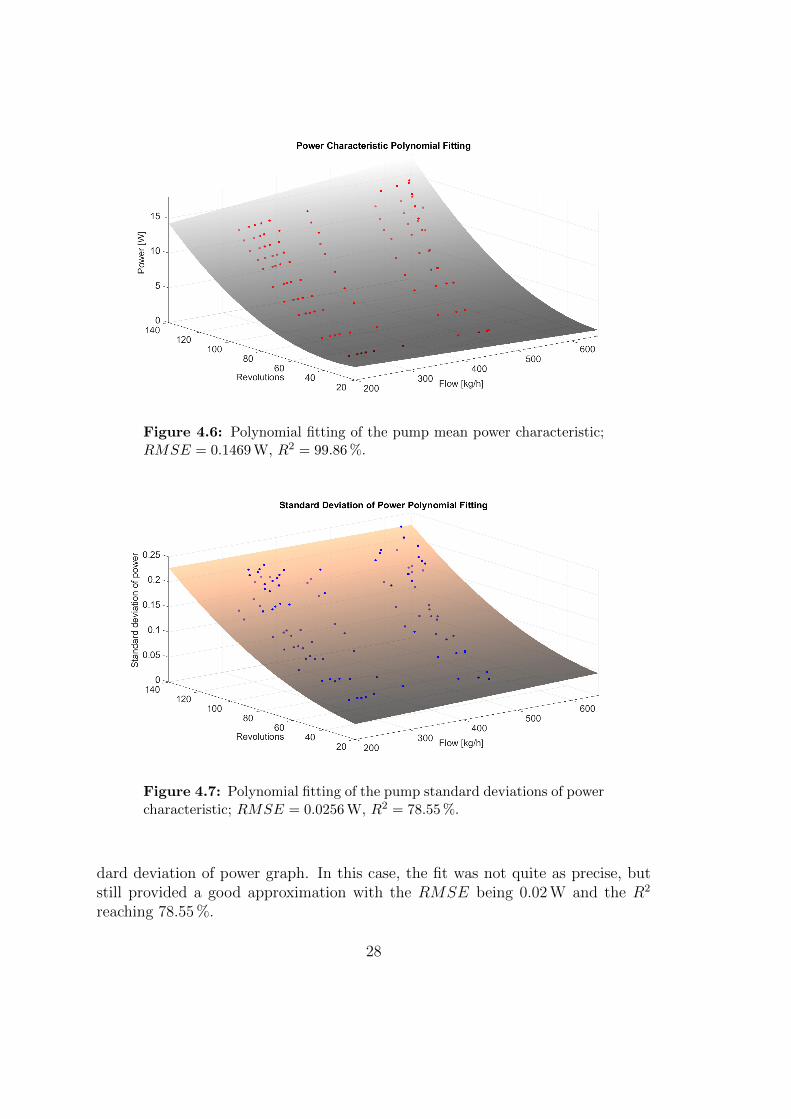
Figure 4.6: Polynomial fitting of the pump mean power characteristic;RMSE = 0.1469 W, R2 = 99.86 %.

Figure 4.7: Polynomial fitting of the pump standard deviations of powercharacteristic; RMSE = 0.0256 W, R2 = 78.55 %.

dard deviation of power graph. In this case, the fit was not quite as precise, butstill provided a good approximation with the RMSE being 0.02 W and the R2

reaching 78.55 %.

28

4.2 Simulink Model

To be able to run simulations of the hydronic system, I used a Simulink model.However, instead of creating a model from scratch, I worked with an existingSimulink test-bench previously created by my colleagues at the Department ofControl Engineering, which I adjusted extensively to fit my needs.

The Simulink test-bench is constituted by a primary and a secondary hydroniccircuit, with only the primary being relevant to my needs. The primary circuitconsists of two parts: the hydraulic part and the thermal part. The thermal partwhich mainly includes the boiler is not very important for my goals either. Thecrucial part is in fact the hydraulic part, as it encompasses everything importantfor the mass flow. There is a model of a pump, a resistance and it also includesthe dynamics of inertance.

4.2.1 Pump Electric Power Model

The first important addition to the hydronic model was the electric powermodel of the pump. Since the most important information for the mass flowestimator comes from the measurement of the electric power supplied to the pump,the model needs to somehow emulate it. To do so is the purpose of the pumpelectric power model.

The result of the pump analysis described in the previous section was a poly-nomial fitted to the electric power characteristic of the pump. Because there isno actual electric power which would drive the pump in the Simulink model andwhich could be observed, it has to be estimated based on this characteristic. Fig-ure 4.8 illustrates the procedure. The current simulated mass flow, which is aknown quantity throughout the simulation, and the current pump speed, which isalso known during simulation and easily precisely measured in a real system, serveas the input information. A two dimensional flow-power characteristic appropri-ate at the given pump speed is first selected from the polynomial. The mass flowvalue is then transformed using this characteristic to the expected mean value ofthe electric power.

To imitate the statistical properties of the real power measurement, the knowl-edge of the standard deviation is then used. The appropriate value of standarddeviation is first picked out by evaluating the polynomial fitted to the standarddeviation of power in a similar fashion in which it has been done with the powermean. The transformed mean value is then obfuscated by adding a random noisewhich has this appropriate standard deviation to it.

29

Flow [kg/h]0 200 400 450.10 600

Pow

er [W

]

4

6

7.578

10

100 revs/s

µσ

σ

90 revs/s

95 revs/s

105 revs/s

110 revs/s

µ

Flow to Power Transformation

Figure 4.8: Flow to power transformation. Transformed mean value ismarked by µ; transformed value at the distance of one standard deviationfrom the mean value is marked by σ.

Going back to the Simulink model, as shown on Figure 4.9, it takes in the massflow and the revolutions values as inputs and evaluates the two fitted polynomialsbased on these inputs. The results of the evaluations are then combined, with theuse of a generated normally distributed random number.

With the ability to produce measurements of electric power now added to thesimulator, it is a good representation of a real hydronic system test-bench. Itcontains everything that I need to test a mass flow estimator. In the followingchapter, I deal with designing such an estimator.

30

Flow (x)

Revolutions (y)

ModelTerms

Coeff icients

Power

Power Characteristic Evaluation

Flow (x)

Revolutions (y)

ModelTerms

Coeff icients

Std Deviation

Std Deviation of Power Evaluation

RandomNumber

Add

Product

[5x2]

Pwr Model Terms [1x5]

Pwr Coefficients

[5x2]

Std Model Terms [1x5]

Std Coefficients

1Power Estimate1

Flow

2Revolutions

Noise

Figure 4.9: Pump electric power model schema. The model evaluatesthe polynomial fitted to the power characteristic giving an estimate of theelectric power measurement.

31

32

Chapter 5

Mass Flow Estimator

In this chapter, I discuss my implementation of the mass flow estimator. Istart of with a simple measurement based Kalman filter estimator, which has noknowledge of the system dynamics. Later, I build on it to create the final estimator,which is essentially an extended Kalman filter (EKF), which utilizes a state-spacemodel. In the process, I overview the resources I used when implementing the EKFin MATLAB and later in Simulink. I also deal with the numerical robustness ofmy implementation of the EKF, taking advantage of alternative implementationmethods.

5.1 MATLAB Toolbox

The first step in the creation of the mass flow estimator is implementing theKalman filter itself. Thankfully, this has already been done by many others, so Ican build on the fruits of their work. A nice toolbox for Kalman filtering, whichI have initially chosen to work with, has been created by Simo Sarka, et al. atthe Aalto University School of Science [18]. It is called the EKF/UKF Toolboxfor MATLAB and it focuses mainly on the extended and unscented versions ofKalman filters and Kalman smoothers. It however also considers regular Kalmanfilters and provides many miscellaneous functions for discretization of linear sys-tems, probability calculations, etc. Several demo problem solutions demonstratingthe functionality of the toolbox are also included—a detail which was of greatimportance and help in my work.

The main functionality of the toolbox is provided in the functions calculatingthe temporal update and the measurement update of a Kalman filter. The toolbox

33

includes several versions of these functions, one for each version of the Kalman fil-ter it considers. As an example, for the linear Kalman filter, there is a functionkf predict which performs the temporal update and a function kf update whichperforms the measurement update. Analogously, for the extended Kalman fil-ter using linear approximation, there are the ekf predict1 and the ekf update1

functions. Input parameters of these functions are used to specify the differentvariances as well as model of the system to which the Kalman filter is applied. Anin depth description of all the toolbox capabilities is available in its documenta-tion [18].

5.2 Estimator with Simplified Linear Model

Perhaps the simplest and easiest way to implement an estimator lies in usinga regular linear Kalman filter, which would operate without any knowledge of thenon-linear model of the system. The only information such a Kalman filter usesis a noisy measurement of the observed variable, which is in this case the electricpower. However, because the observed output equation for electric power (??) isnot linear and I want to use a linear filter at this stage, I instead transform thenoisy measurement of the electric power driving the pump to mass flow using theP-q characteristic of the pump (see Figure 4.5). This is essentially the reverse of theprocess used to model the electric power in the Simulink model (see Figure 4.8). Inthe Simulink test-bench, this transformation of the measurement of electric powerto the mass flow is done at run-time by the flowEstimator block.

The temporal update step of this Kalman filter is based on the assumption,that the update of the state variables is entirely stochastic, following the equation

x−k+1 = xk + vk (5.1)

where v is the random process noise. As is clear from equation (5.1) the state ma-trix A is in this case in fact an identity matrix, meaning that the a priori estimateof the state in mean value remains unchanged, only its uncertainty increases. Thisleaves the bulk of the correction of the value to the measurement update step of theKalman filter, making the estimate thoroughly dependent on the measurementsthem self.

An estimator like this generally does not perform very well compared to anestimator with knowledge of the model. However, in case that the estimatedstates do not change rapidly and the measurements are not biased it performssufficiently well. In steady state situations especially, it can perform almost asgood as the more advanced estimators, which I discuss further on.

34

5.3 Extended Kalman Filter Estimator

The logical improvement over the simple Kalman filter estimator described inthe previous section is taking advantage of the knowledge of the non-linear systemmodel, which is discussed in detail in Appendix B. With the complete state-spacemodel of the system from the appendix, including the calculated Jacobians, I haveall the theory I need to create the improved mass flow estimator. Since this modelis a non-linear one, the use of an extended Kalman filter is necessary.

When using the EKF/UKF toolbox, the transition from a linear Kalman filterto the extended Kalman filter is very simple, the substitution of different temporaland measurement update functions being essentially the only thing required to doso. However, the inclusion of the system model presents more work, as both thefunction f relating the state at the previous time step to the state at the currenttime step and the function h relating the current state to the current measurementneed to be implemented as a MATLAB functions together with functions evaluat-ing their respective Jacobian matrices. Handles to these MATLAB functions arepassed to the toolbox functions during estimation for it to be able to calculate thetemporal and measurement updates.

After the above has been done, the variance matrices describing the processand measurement noise needed to be set. The variance of the measurement ofthe electric power driving the pump have been examined previously in Chapter 4,where I have fitted the standard deviation characteristic with a polynomial. Theestimator evaluates this polynomial at each time step based on the current inputand last estimated state values, so that the variance matrix can be adjusted ac-cordingly. The variance for the process noise has been set empirically with the helpof the Simulink model, which is a common practice when implementing Kalmanfilters. Having done that, the extended Kalman filter estimator which uses all theinformation available to it is ready to be used.

5.3.1 Numerically Robust Implementation

During development and testing of the non-linear estimator, I often ran intotrouble when the calculation of the covariance matrix diverged for various reasons,such as inaccuracies in the model or very noisy input data. Having suspected thatthis was due to numerical inaccuracies caused by round-off errors, I looked forways to reduce the sensitivity of the calculations to such errors, reducing the like-lihood of such issues in the process. I found the solution in employing alternativeimplementation methods for the functions performing the temporal update and

35

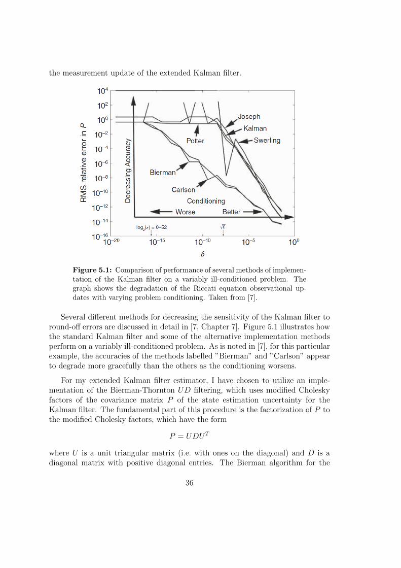
the measurement update of the extended Kalman filter.

Figure 5.1: Comparison of performance of several methods of implemen-tation of the Kalman filter on a variably ill-conditioned problem. Thegraph shows the degradation of the Riccati equation observational up-dates with varying problem conditioning. Taken from [7].

Several different methods for decreasing the sensitivity of the Kalman filter toround-off errors are discussed in detail in [7, Chapter 7]. Figure 5.1 illustrates howthe standard Kalman filter and some of the alternative implementation methodsperform on a variably ill-conditioned problem. As is noted in [7], for this particularexample, the accuracies of the methods labelled ”Bierman” and ”Carlson” appearto degrade more gracefully than the others as the conditioning worsens.

For my extended Kalman filter estimator, I have chosen to utilize an imple-mentation of the Bierman-Thornton UD filtering, which uses modified Choleskyfactors of the covariance matrix P of the state estimation uncertainty for theKalman filter. The fundamental part of this procedure is the factorization of P tothe modified Cholesky factors, which have the form

P = UDUT

where U is a unit triangular matrix (i.e. with ones on the diagonal) and D is adiagonal matrix with positive diagonal entries. The Bierman algorithm for the

36

measurement update and the Thornton algorithm for the temporal update in theRiccati equation are then used on the modified Cholesky factors U and D.

Incorporating these methods into the workflow of the estimator effectivelymeans replacing the functions performing temporal and measurement update fromthe EKF/UKF Toolbox (i.e. the functions ekf predict1 and ekf update1) byfunctions performing the pair of algorithms described above and prepending themby a function performing the initial UD factorization of the covariance matrix.After this has been done, I had an alternative implementation of the extendedKalman filter estimator, which is more likely to produce accurate results even ifthe conditioning of the estimation problem becomes bad, although it is theoret-ically not any better than the standard implementation, if it were to run on acomputer with infinite precision.

5.4 Simulink S-Function

To be able to use the estimator at simulation runtime so that it is be able toperform the estimation on-line, I needed to implement it as a Simulink S-Function.S-Functions provide a way to embed complex code into a Simulink model. Sinceall the previously written code was in MATLAB, I used the Level-2 MATLABS-Functions, which allow for creation of custom blocks with multiple input andoutput ports and capable of handling any type of signal produced by a Simulinkmodel using the MATLAB language.

The working principle of the implemented S-Function is such, that it storesthe mean values and covariance matrix UD factors of the estimated states. Thesestored variables are then updated at each simulation time step using the cur-rent input values according to the MATLAB functions implementing the extendedKalman filter described in the previous section. The estimated means of the statesas well as the corresponding estimated output value are then channelled to the out-put of the Simulink block. These output values are ready to be used for evaluationof the estimator performance and, more importantly, for the purpose of control ofmass flow in the hydronic system.

Performance of the implemented mass flow estimator is examined in Chapter 7.Before that however, the next chapter deals with the control of mass flow in thehydronic system.

37

38

Chapter 6

Control

The next goal of this thesis, now that the mass flow estimator has been devel-oped, is to utilize the estimation in an optimal mass flow controller which wouldfollow some input (reference) mass flow. To control the mass flow, the pump driv-ing the liquid in the hydronic system needs to be controlled, so in this chapter,I develop a controller for the pump. First, I use a simple PI feedback controller.After that, I try to develop a more complex controller utilizing optimal controltechniques.

6.1 PI Controller

The proportional-integral (PI) controller is a special case of the proportional-integral-derivative (PID) controller without the derivative term. The workingprinciple of the controller is very simple. It continuously calculates the differ-ence between a desired reference setpoint and a measured process variable. Thisdifference is called the error. The controller attempts to minimize this error overtime by adjusting its control output, which is calculated as a sum of the errorand its integral weighted by the proportional and the integral gains respectively.Expressed in an equation, the control output of the PI controller is calculated as

u(t) = Kpe(t) +Ki

∫ t

0

e(τ) dτ (6.1)

where t is the present time, e(t) is the error, Kp is the proportional gain and Ki isthe integral gain.

In the hydronic system in question, there is no direct measurement of thecontrolled variable—the mass flow—so it is not possible to calculate the error

39

in the usual way. Instead of the measurement, I use the estimate of mass flowprovided by the mass flow estimator developed earlier in this thesis. A schema ofthe hydronic system being controlled by a PI controller is shown on Figure 6.1.The tuning of the PI controller parameters was done by hand. The reason for itbeing that there is not a systematic way for tuning it for non-linear systems.

Figure 6.1: Schema of the hydronic system with PI Controller. Thedesired mass flow setpoint is denoted qref , while q and q denote the massflow estimate and the actual mass flow in the system respectively. Themeasured electric power Pe is obscured by a measurement error em. Thecontroller output is the pump speed s.

The disadvantage of using the PI controller in this scenario is that it doesnot use the knowledge of the hydronic system model in any way. Even though itworks reasonably well, as will be shown in the next chapter, I now look for a wayof utilizing this knowledge in the creation of a better controller.

6.2 Jacobian Linearization Based Controller

When attempting to control a non-linear system, it is possible to use anapproach called Jacobian linearization of a non-linear system about the trajec-tory [19]. In this approach I use a feedforward controller calculating the steadystate input of the system based on the reference mass flow. The trajectory of thefeedforward controller is the used for the linearization. Once the linearization isdone, it is possible to use the result to design an optimal linear-quadratic regulator(LQR), which is a form of state-feedback controller.

40

6.2.1 Jacobian Linearization

Considering a non-linear system governed by the equation

xk+1 = f(xk,uk) (6.2)

a point x is called an equilibrium point if there is a specific equilibrium input u,such that

f(x, u) = 0 (6.3)

Since (x, u) is an equilibrium point and input, it is guaranteed, that if the systemstarts at x0 = x and the constant input uk = u, then the state of the system willremain fixed at xk = x for all time steps k.

Defining deviation variables, allows for describing what happens in case thesystem deviates from the equilibrium a little.

δxk = xk − x

δuk = uk − u

Substituting the deviation variables into the differential equation (6.2) yields

δxk+1 = f(δxk, δuk) (6.4)

Doing first order Taylor expansion of of the right hand side of equation (6.4)results in

δxk+1 ≈ f(x, u) +∂f

∂x

∣∣∣∣x = xu = u

δxk +∂f

∂u

∣∣∣∣x = xu = u

δuk (6.5)

Remembering, that f(x, u) = 0 leaves

δxk+1 ≈∂f

∂x

∣∣∣∣x = xu = u

δxk +∂f

∂u

∣∣∣∣x = xu = u

δuk (6.6)

The difference equation (6.6) approximately governs the deviation variables δx k

and δu k as long as they remain small.

Looking closely at the partial derivatives in equation (6.6), one can notice, thatwhen considering the hydronic system at hand the first one is actually the stateequation Jacobian F introduced and derived in Appendix B (or more precisely itsfirst element, since I am only controlling the mass flow) evaluated at the equi-librium. Defining the second partial derivative in equation (6.6) to be anotherJacobian G = ∂f

∂u

∣∣x = xu = u

one can write

δxk+1 = Fδxk + Gδuk (6.7)

41

Equation (6.7) is called the Jacobian linearization of the original non-linear sys-tem about the equilibrium point (x, u) which for small deviations approximatelygoverns the relationship between the deviation variables δx and δu.

The above works well for simple cases. However, it is not satisfactory for thecontrol of the hydronic system, where the deviations are relatively large. Thank-fully a generalization of this approach exists. It lies in redefining the Jacobianmatrices as being time-varying

Fk =∂f

∂x

∣∣∣∣xk = xk

uk = uk

Gk =∂f

∂u

∣∣∣∣xk = xk

uk = uk

Having done that, the governing difference equation changes to

δxk+1 = Fkδxk + Gkδuk (6.8)

This new equation (6.8) is called the Jacobian linearization of the system about thetrajectory and acts as a generalization of the linearizations about the equilibriumpoints [19].

6.2.2 Feedforward Controller

To bring the system close to the desired reference fast and to create a trajectoryfor the Jacobian linearization, I design a feedforward controller calculating thesteady state control input necessary for the reference state. This can be donesimply by solving for s in the equation

0 =a2 −RI

q2 +a1Isq +

a0Is2 (6.9)

which is the equation (3.15) with the rate of change of mass flow q equal to zero.I denote the solution to this steady state equation sff .

6.2.3 Linear-quadratic Regulator

Utilizing the result of Jacobian linearization, I now design a linear-quadraticregulator. In essence, the LQR algorithm is a way of designing an optimal state-feedback controller to drive the deviation variables to zero. Generally, given alinear system

xk+1 = Axk + Buk

42

the algorithm calculates an optimal gain matrix K such that the state-feedbacklaw

uk = −Kxk (6.10)

minimizes the quadratic performance measure

J =∞∑k=0

(xTk Qxk + uT

k Ruk

)(6.11)

where Q is a real symmetric positive semi-definite matrix and R is a real symmetricpositive definite matrix [20].

In my case, I only have a linear equation for the deviation variables

δxk+1 = Fkδxk + Gkδuk

so the state-feedback law takes the form of

δuk = −Kδxk (6.12)

and it minimizes the performance measure

J =∞∑k=0

(δx

Tk Qδxk + δu

Tk Rδuk

)(6.13)

Thus, this state-feedback clearly only takes care of the deviations from the trajec-tory, i.e. deviations from the reference.

Adding together the feedforward control sff and the LQR state-feedback con-trol sLQR = δuk evaluated at the reference mass flow and the corresponding inputprovided by the feedforward controller forms the entire control input regulatingthe non-linear system. The schema shown on Figure 6.2 shows the layout of theentire Jacobian linearization based control complete with the EKF mass flow esti-mator, the feedforward controller calculating the steady state input and the LQRstate-feedback accounting for any deviations.

6.2.4 Gain Scheduling

The first implementation of the controller described above has been written asusing Level-2 MATLAB S-Functions, which evaluated of all the necessary calcu-lations directly at runtime. Due to the relative complexity of these calculation,especially those necessary for the LQR algorithm, the simulations ran quite slowly.

43

Figure 6.2: Schema of the hydronic system with Feedforward and LQRController. EKF estimator provides estimates of mass flow q and hy-draulic resistance R based on the measurements of electric power Pe.These are utilized in the feedforward controller and the LQR state-feedback controller to provide control input back to the hydronic systembased on reference mass flow qref .

To circumvent this issue, I chose to take advantage of the gain scheduling tech-nique.

The basis of this technique lies in replacing the computationally demandinglinearization and optimal gain calculations by the use of pre-computed values ofthe gain. The gain values are first calculated off-line for a number of possible stateand input values, which are uniformly distributed within the operating space ofthe system. These values are then interpolated and used as a ”schedule” or lookuptable during simulation.

The schedule of K for the LQR state-feedback controller used in my imple-mentation is shown on Figure 6.3. Even though the use of such schedule meanslosing some precision compared to the direct calculation approach, with reason-able density of the pre-calculated schedule, it is easily outweighed by the benefitof radically increased simulation speed.

With controller design finished, I can finally proceed to the evaluation of theperformance of the estimator as well as the performance of the controllers them-selves.

44

250200

150

Flow [kg/h]100

LQR Gain Schedule

500

0.20.4

Revolutions

0.60.8

0

0.1

0.2

0.3

1

K

Figure 6.3: LQR gain schedule. A graph showing the pre-calculatedvalues of the LQR gain K for different values of mass flow and pump rev-olutions uniformly distributed around the operating space of the system.

45

46

Chapter 7

Experiments

In this chapter, I present the experimental results of the designed mass flowestimator and the developed mass flow controller. All the presented experimentswere performed on the simulation model of the hydronic system implemented inSimulink. A physical model of the hydronic system has unfortunately not beenavailable for comparison. I begin with the review of performance of the mass flowestimator, after which I move on to the mass flow controller.

7.1 Mass Flow Estimation

For the evaluation of mass flow estimation, I did not use any form of a con-troller in the simulation model. Instead, I directly set up the pump speed inputwith a series of predefined setpoints. Since the hydraulic resistance in the systemis constant, this means that after a each setpoint had been set, the mass flowwere constant as well once the transients had died out until a new setpoint wasintroduced.

7.1.1 Estimator with Simplified Linear Model

The first experiment I ran, was with the Simplified Linear Model Estimator.This estimator has no knowledge of the non-linear model and uses measurementsof electric power transformed to mass flow by the P-q characteristic as a base forits estimate. As can be seen on Figure 7.1, such estimator works reasonably wellfor high flow situations. However, its performance when the mass flow becomeslower is completely unsatisfactory.

47

Time [s]0 10 20 30 40 50 60 70 80

Flo

w [k

g/h]

50

100

150

200

250Simplified Linear Model Estimator: Mass Flow Estimation

Observed power transformed to mass flowSimulated mass flowKalman filter estimate of mass flow

Figure 7.1: Mass flow estimation using the simplified linear model esti-mator. The estimate eventually gets close to the real value of mass flowwhen it is high, but fails to do so very precisely, when it is low.

Part of the reason for the poor performance is due to the estimator not takinginto account the changes of variance in the data for different values of mass flow.Adding this feature could somewhat lower the fluctuation of the estimate, eventhough it would not cure it completely. However, even when the flow is higher,the time it takes the estimator to converge to the correct value of mass flow isrelatively high.

7.1.2 Extended Kalman Filter Estimator

The more complex extended Kalman filter estimator with knowledge of thenon-linear system performs much better. Obtaining information directly from themeasurement of power, the estimator is able to estimate the true mass flow veryprecisely, as can be seen on Figure 7.2. The estimated mass flow is within 1 kg/hof the true simulated value.

The EKF estimator does not suffer from the imprecision in low mass flowsituations as the simple estimator did. Thanks to the fact, that the mathematicalmodel in the estimator fits closely to the model used in the simulation, the estimatealso follows any changes in mass flow due to changes in input pump speed veryprecisely.

Figure 7.3 show, that the extended Kalman filter estimator also does a good

48

Time [s]0 10 20 30 40 50 60 70 80

Flo

w [k

g/h]

50

100

150

200

250EKF Estimator: Mass Flow Estimation

True simulated mass flowEstimated mass flow

Figure 7.2: Mass flow estimation using the extended Kalman filter es-timator.

job filtering the noisy electric power measurement. The estimate of electric poweris very smooth even when the variance of noise in the measurements is relativelyhigh.

As opposed to the simple estimator, the EKF estimator is also able to identifyand estimate the hydraulic resistance of the hydronic system quite precisely with-out any initial knowledge about it. Figure 7.4 shows that the estimate of resistanceis very close to the true value. Nevertheless, the resistance is not estimated abso-lutely precisely and some of the disparity between the estimated and the actualtrue mass flow is in fact due to this imprecision.

The certainty the estimator has about its estimation is reflected in the mass flowstandard deviation calculated from the internal Kalman filter covariance matrixand shown in Figure 7.5. The plot clearly shows, that after some initial uncertainty,the standard deviation stays approximately below 2 kg/h. The root-mean-squareerror of the estimation was in fact in this case 1.12 kg/h. This makes the estimatorvery precise with the estimation error two orders of magnitude smaller than theactual mass flow value.

Overall the results of the extended Kalman filter estimator are very satisfactoryand mean a significant improvement over the simple estimator used initially. Assuch, they also serve as good base for the next step—experiments with the massflow control.

49

Time [s]0 10 20 30 40 50 60 70 80

Ele

ctric

pow

er [W

]

0

2

4

6

8

10

12EKF Estimator: Electric Power

Measured powerEstimated power

Figure 7.3: Electric power measurements acting as the main source ofinformation for the extended Kalman filter estimator.

Time [s]0 10 20 30 40 50 60 70 80R

esis

tanc

e [P

a h2 /k

g2 ]

0

0.1

0.2EKF Estimator: Resistance Estimation

True simulated resistanceEstimated resistance

Figure 7.4: Hydraulic resistance estimated by the extended Kalmanfilter estimator compared to its true value.

Time [s]0 10 20 30 40 50 60 70 80F

low

est

im. s

td [k

g/h]

0

5

10EKF Estimator: Flow Estimation Standard Deviation

Flow estimation standard deviation

Figure 7.5: Standard deviation of mass flow calculated from the internalcovariance matrix of the extended Kalman filter estimator expresses howcertain the estimator is about its estimate.

50

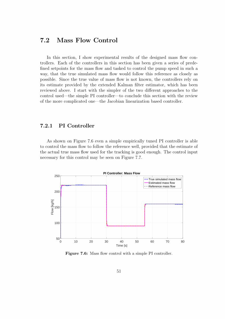
7.2 Mass Flow Control

In this section, I show experimental results of the designed mass flow con-trollers. Each of the controllers in this section has been given a series of prede-fined setpoints for the mass flow and tasked to control the pump speed in such away, that the true simulated mass flow would follow this reference as closely aspossible. Since the true value of mass flow is not known, the controllers rely onits estimate provided by the extended Kalman filter estimator, which has beenreviewed above. I start with the simpler of the two different approaches to thecontrol used—the simple PI controller—to conclude this section with the reviewof the more complicated one—the Jacobian linearization based controller.

7.2.1 PI Controller

As shown on Figure 7.6 even a simple empirically tuned PI controller is ableto control the mass flow to follow the reference well, provided that the estimate ofthe actual true mass flow used for the tracking is good enough. The control inputnecessary for this control may be seen on Figure 7.7.

Time [s]0 10 20 30 40 50 60 70 80

Flo

w [k

g/h]

50

100

150

200

250PI Controller: Mass Flow

True simulated mass flowEstimated mass flowReference mass flow

Figure 7.6: Mass flow control with a simple PI controller.

51

Time [s]0 10 20 30 40 50 60 70 80P

ump

spee

d [r

evs/

s]

0

50

100

PI Controller: Pump Speed

Pump revolutions

Figure 7.7: Pump speed control input determined by the PI controller.

7.2.2 Jacobian Linearization Based Controller

The results of the much more complex control based on Jacobian linearizationand incorporating a feedforward controller and an LQR state-feedback controllerare shown on Figures 7.8 and 7.9.

Time [s]0 10 20 30 40 50 60 70 80

Flo

w [k

g/h]

50

100

150

200

250FF+LQR Controller: Mass Flow

True simulated mass flowEstimated mass flowReference mass flow

Figure 7.8: Mass Flow control with the feedforward and LQR controller.

While it certainly does show an improvement over the simple PI controller, it isnot a very substantial one. The complex controller does achieve the setpoint fasterand does so using somewhat smoother control input (i.e. with smaller spike at thetransition between setpoints). However, its towering complexity when comparedto the PI controller, makes the latter preferable in situations, where fast transitionsare not a vital requirement.

52

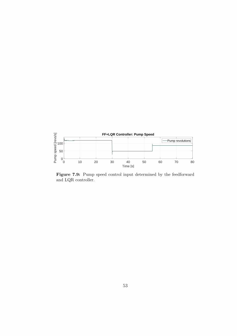
Time [s]0 10 20 30 40 50 60 70 80P

ump

spee

d [r

evs/

s]

0

50

100

FF+LQR Controller: Pump Speed

Pump revolutions

Figure 7.9: Pump speed control input determined by the feedforwardand LQR controller.

53

54

Chapter 8

Conclusion

In this thesis, I have dealt with mass flow in hydronic systems. My goal hasbeen to develop a simulation model of a hydronic system consisting of a pump anda heat exchanger and to develop a mass flow estimator for this setup. The massflow estimator was supposed to fuse all available information to make estimates ofmass flow through the pump. The next goal of this work was to develop a massflow controller for the system using optimal control techniques.

I began with a theoretical study of data fusion and estimation theory, re-viewing several methods of state estimation applicable to hydronic systems. Themethod which I chose to use for the design of the mass flow estimator—the Kalmanfiltering—was analysed in more detail.

The theory of hydronic system modelling was the next subject of my focus.I first derived a mathematical model of each of the components of the hydronicsystem separately, with extra focus on the model of the pump, before joiningthem together into a mathematical model of the complete hydronic system. Thismathematical model served as a foundation for the setup of simulation modelimplemented in Simulink. I used data recorded from a physical model of a hydronicnetwork to calibrate the simulation model of the pump. I also used the data for thestudy of pump electric power characteristic with respect to mass flow and pumpimpeller revolutions. I fitted the data with a multidimensional polynomial for lateruse in the estimation.

In the design of the mass flow estimator I first derived the discrete version ofthe mathematical model of the hydronic system. I then used this discretized modelto formulate a state-space description of the non-linear system. This state-spacedescription was then used in an extended Kalman filter which performed the actualestimation. After that, I augmented the state-space description with the hydraulic

55

resistance parameter, for the Kalman filter to be able to estimate it together withthe mass-flow. This not only increased the reliability of the estimation, but alsoremoved the need for the resistance to be identified in some other way.

When implementing the mass flow estimator, I first created a version relyingsolely on the data and the electric power-to-mass flow characteristic of the pump.Then, I improved upon it by incorporating the non-linear model and by the useof the extended Kalman filter. In the final version of the estimator, I utilized analternative implementation method of the Kalman algorithm robust to round-offerrors, which uses modified Cholesky factors of the covariance matrix, to increasethe overall precision.

Finally, I created a mass flow controller which uses the mass flow estimateto track a reference mass flow setpoint. I present two alternative versions of thecontroller, the first being a simple PI controller, the other a more complex Jacobianlinearization based controller, which consists of a feedforward part and an optimalLQR state-feedback controller for control of the deviations from the trajectory.

Simulation experiments with the estimators presented towards the end of thisthesis show that the extended Kalman filter mass flow estimator performs verywell. Its precision stands out especially when compared with the simple linearestimator relying solely on the data. In my experiments, the estimation error wastwo orders of magnitude smaller than the estimated value. Thanks to the goodperformance of the estimator, it is possible to control the mass flow even with a verysimple PI controller as is illustrated by the experiments. Comparing the complexJacobian linearization based controller with the optimal LQR state-feedback tothe PI controller shows, that little improvement of the control is actually achievedby its usage.

Unfortunately, I was unable to verify the performance of the mass flow estima-tor and the mass flow controller on a physical model of the hydronic system, asa suitable test-bench has not been made functional in time. However, other thanthat, I fulfilled every task given to me in the assignment.

Thus, the component on which future improvements should concentrate pri-marily is the mass flow estimator rather than the mass flow controller. Possibleextensions of the estimator include the inclusion of information coming from thetemperature drop across the heat exchanger in the estimation. Such informationwould make the estimator more robust towards imprecisions of the dynamic modelof the mass flow and the possible discrepancy between the modelled pump and re-ality. As for the controller, the use of non-linear model predictive control mightbe feasible. However, as it has been shown that even a simple PI controller givessatisfactory results, it might not bring a significant improvement.

56

Bibliography

[1] J. R. Raol, Multi-Sensor Data Fusion with MATLAB R©. CRC Press, 2009.

[2] F. Castanedo, “A review of data fusion techniques,” The Scientific WorldJournal, vol. 2013, 2013.

[3] M. S. Landy, L. T. Maloney, E. B. Johnston, and M. Young, “Measurementand modeling of depth cue combination: in defense of weak fusion,” Visionresearch, vol. 35, no. 3, pp. 389–412, 1995.

[4] F. E. White, “Data fusion lexicon,” tech. rep., DTIC Document, 1991.

[5] G. Welch and G. Bishop, “An Introduction to the Kalman Filter: SIGGRAPH2001 Course 8,” in Computer Graphics, Annual Conference on ComputerGraphics & Interactive Techniques, pp. 12–17, 2001.

[6] R. E. Kalman, “A new approach to linear filtering and prediction problems,”Transactions of the ASME–Journal of Basic Engineering, vol. 82, no. SeriesD, pp. 35–45, 1960.

[7] M. S. Grewal and A. P. Andrews, Kalman Filtering: Theory and PracticeUsing MATLAB. John Wiley & Sons, Inc., 2014.

[8] C. Sullivan, “Lumped fluid systems.” http://www.dartmouth.edu/

~sullivan/22files/Fluid%20sys%20anal%20w%20chart.pdf, 2004.

[9] Grundfos, The Centrifugal Pump. Grundfos Research and Technology, 2008.

[10] J. Dostal, “Decentralized control of hydronic building systems.” An unpub-lished Doctoral Study Report, January 2015.

[11] F. Frishman, On the Arithmetic Means and Variances of Products and Ratiosof Random Variables, pp. 401–406. Dordrecht: Springer Netherlands, 1975.

[12] MathWorks, “Chi-square goodness-of-fit test — MATLAB documentation.”http://www.mathworks.com/help/stats/chi2gof.html, 2016. [Online; ac-cessed 4 September 2016].

57

[13] MathWorks, “Lilliefors test — MATLAB documentation.” http://www.

mathworks.com/help/stats/lillietest.html, 2016. [Online; accessed 4September 2016].

[14] MathWorks, “One-sample t-test — MATLAB documentation.” http://www.

mathworks.com/help/stats/ttest.html, 2016. [Online; accessed 4 Septem-ber 2016].

[15] L. Wasserman, All of Statistics: A Concise Course in Statistical Inference.Springer Science & Business Media, 2013.

[16] N. M. Razali, Y. B. Wah, et al., “Power comparisons of Shapiro-Wilk,Kolmogorov-Smirnov, Lilliefors and Anderson-Darling tests,” Journal of Sta-tistical Modelling and Analytics, vol. 2, no. 1, pp. 21–33, 2011.

[17] J. R. D’Errico, “Polyfitn.” https://www.mathworks.com/matlabcentral/

fileexchange/34765-polyfitn, 2016. [Online; accessed 4 September 2016].

[18] S. Sarkka, J. Hartikainen, and A. Solin, Optimal Filtering with Kalman Filtersand Smoothers: a Manual for the Matlab toolbox EKF/UKF. Aalto UniversitySchool of Science, 1.3 ed., 2011.

[19] A. Packard, K. Poolla, and R. Horowitz, “Dynamic systems and feedback.”http://www.cds.caltech.edu/~murray/courses/cds101/fa02/caltech/

pph02-ch19-23.pdf, 2002.

[20] D. E. Kirk, Optimal Control Theory: An Introduction. Courier Corporation,2004.

[21] W. Press, B. Flannery, S. Teukolsky, and W. Vetterling, Numerical Recipesin FORTRAN 77: The Art of Scientific Computing, Volume 1 of FortranNumerical Recipes. Numerical Recipes in FORTRAN: The Art of ScientificComputing, Cambridge University Press, 1992.

[22] E. W. Weisstein, “Euler Forward Method. From MathWorld–A WolframWeb Resource..” http://mathworld.wolfram.com/EulerForwardMethod.

html, 2016. [Online; accessed 30 November 2016].

[23] P. J. Smith, Joint state and parameter estimation using data assimilation withapplication to morphodynamic modelling. PhD thesis, University of Reading,2010.

[24] G. Plett, “Dual and joint EKF for simultaneous SOC and SOH estimation,” inProceedings of the 21st Electric Vehicle Symposium (EVS21), Monaco, pp. 1–12, 2005.

58

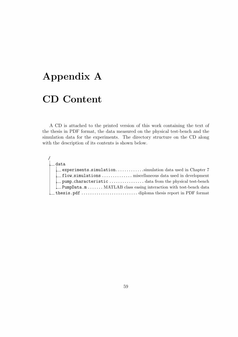
Appendix A

CD Content

A CD is attached to the printed version of this work containing the text ofthe thesis in PDF format, the data measured on the physical test-bench and thesimulation data for the experiments. The directory structure on the CD alongwith the description of its contents is shown below.

/

data

experiments simulation.............simulation data used in Chapter 7

flow simulations ..............miscellaneous data used in development

pump characteristic ................ data from the physical test-bench

PumpData.m .......MATLAB class easing interaction with test-bench data

thesis.pdf .......................... diploma thesis report in PDF format

59

60

Appendix B

Non-linear System Model

Not included due to confidentiality restrictions.

61