Embed Size (px)
DESCRIPTION
dip note
Citation preview
Department of Computer Engineering, CMU
1
Chapter 3
Image Enhancement in the
Spatial Domain
2
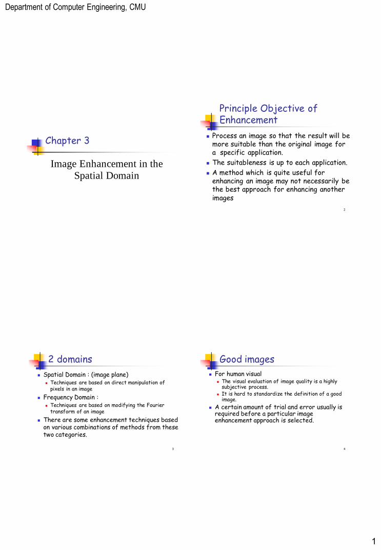
Principle Objective of Enhancement
Process an image so that the result will be more suitable than the original image for a specific application.
The suitableness is up to each application.
A method which is quite useful for enhancing an image may not necessarily be the best approach for enhancing another images
3
2 domains
Spatial Domain : (image plane) Techniques are based on direct manipulation of
pixels in an image
Frequency Domain : Techniques are based on modifying the Fourier
transform of an image
There are some enhancement techniques based on various combinations of methods from these two categories.
4
Good images
For human visual The visual evaluation of image quality is a highly
subjective process. It is hard to standardize the definition of a good
image.
A certain amount of trial and error usually is required before a particular image enhancement approach is selected.
Department of Computer Engineering, CMU
2
5
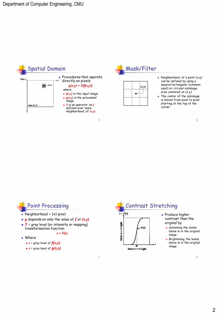
Spatial Domain
Procedures that operate directly on pixels.
g(x,y) = T[f(x,y)]
where
f(x,y) is the input image g(x,y) is the processed
image T is an operator on f
defined over some neighborhood of (x,y)
6
Mask/Filter
Neighborhood of a point (x,y) can be defined by using a square/rectangular (common used) or circular subimage area centered at (x,y)
The center of the subimage is moved from pixel to pixel starting at the top of the corner
•
(x,y)
7
Point Processing
Neighborhood = 1x1 pixel
g depends on only the value of f at (x,y)
T = gray level (or intensity or mapping) transformation function
s = T(r)
Where
r = gray level of f(x,y)
s = gray level of g(x,y)
8
Contrast Stretching
Produce higher contrast than the original by darkening the levels
below m in the original image
Brightening the levels above m in the original image
Department of Computer Engineering, CMU
3
9
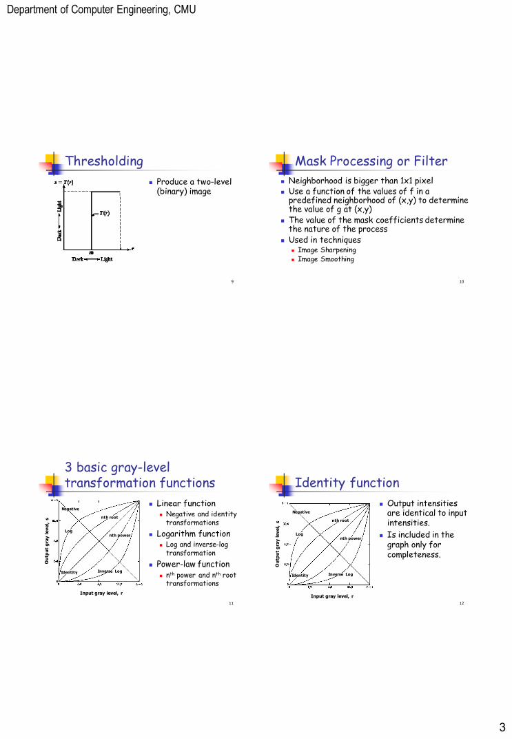
Thresholding
Produce a two-level (binary) image
10
Mask Processing or Filter
Neighborhood is bigger than 1x1 pixel Use a function of the values of f in a
predefined neighborhood of (x,y) to determine the value of g at (x,y)
The value of the mask coefficients determine the nature of the process
Used in techniques Image Sharpening Image Smoothing
11
3 basic gray-level transformation functions
Linear function Negative and identity
transformations
Logarithm function Log and inverse-log
transformation
Power-law function nth power and nth root
transformations Input gray level, r
Negative
Log
nth root
Identity
nth power
Inverse Log
12
Identity function
Output intensities are identical to input intensities.
Is included in the graph only for completeness.
Input gray level, r
Negative
Log
nth root
Identity
nth power
Inverse Log
Department of Computer Engineering, CMU
4
13
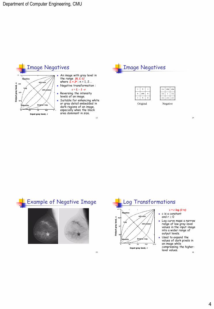
Image Negatives
An image with gray level in the range [0, L-1] where L = 2n ; n = 1, 2…
Negative transformation : s = L – 1 –r
Reversing the intensity levels of an image.
Suitable for enhancing white or gray detail embedded in dark regions of an image, especially when the black area dominant in size. Input gray level, r
Negative
Log
nth root
Identity
nth power
Inverse Log
14
Image Negatives
1 5 1
5 255 5
1 5 0
254 250 254
250 0 250
254 250 255
Original Negative
15
Example of Negative Image
16
Log Transformations
s = c log (1+r)
c is a constant and r 0
Log curve maps a narrow range of low gray-level values in the input image into a wider range of output levels.
Used to expand the values of dark pixels in an image while compressing the higher-level values.
Input gray level, r
Negative
Log
nth root
Identity
nth power
Inverse Log
Department of Computer Engineering, CMU
5
17
Example of Logarithm Image
18
Inverse Logarithm Transformations
Do opposite to the Log Transformations
Used to expand the values of high pixels in an image while compressing the darker-level values.
19
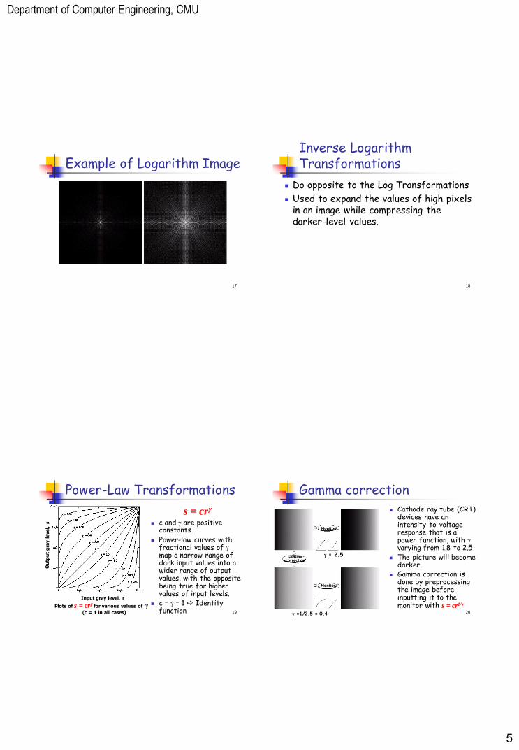
Power-Law Transformations
s = cr c and are positive
constants
Power-law curves with fractional values of map a narrow range of dark input values into a wider range of output values, with the opposite being true for higher values of input levels.
c = = 1 Identity function
Input gray level, r
Plots of s = cr for various values of
(c = 1 in all cases) 20
Gamma correction
Cathode ray tube (CRT) devices have an intensity-to-voltage response that is a power function, with varying from 1.8 to 2.5
The picture will become darker.
Gamma correction is done by preprocessing the image before inputting it to the monitor with s = cr1/
Monitor
Monitor
Gamma correction
= 2.5
=1/2.5 = 0.4
Department of Computer Engineering, CMU
6
21
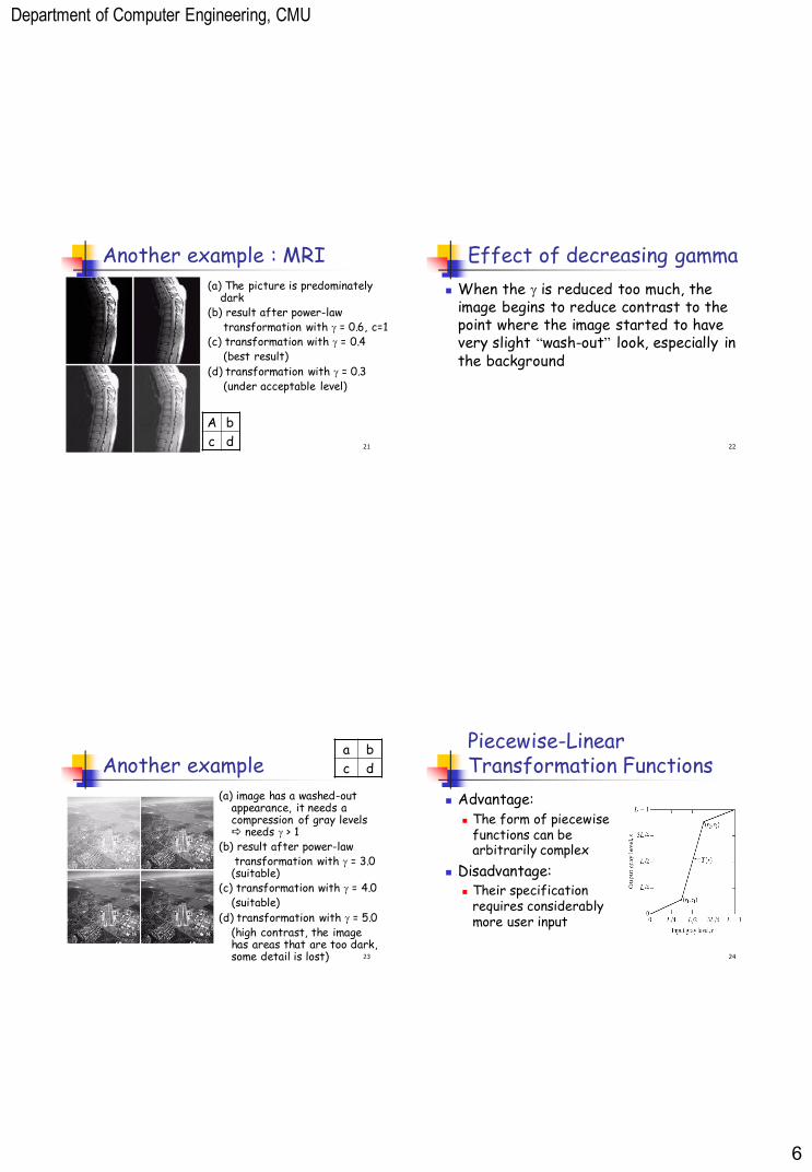
Another example : MRI
(a) The picture is predominately dark
(b) result after power-law transformation with = 0.6, c=1 (c) transformation with = 0.4 (best result)
(d) transformation with = 0.3 (under acceptable level)
A b
c d 22
Effect of decreasing gamma
When the is reduced too much, the image begins to reduce contrast to the point where the image started to have very slight “wash-out” look, especially in the background
23
Another example
(a) image has a washed-out appearance, it needs a compression of gray levels needs > 1
(b) result after power-law transformation with = 3.0
(suitable) (c) transformation with = 4.0 (suitable)
(d) transformation with = 5.0 (high contrast, the image
has areas that are too dark, some detail is lost)
a b
c d
24
Piecewise-Linear Transformation Functions
Advantage: The form of piecewise
functions can be arbitrarily complex
Disadvantage: Their specification
requires considerably more user input
Department of Computer Engineering, CMU
7
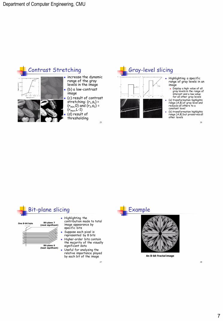
25
Contrast Stretching increase the dynamic
range of the gray levels in the image
(b) a low-contrast image
(c) result of contrast stretching: (r1,s1) = (rmin,0) and (r2,s2) = (rmax,L-1)
(d) result of thresholding
26
Gray-level slicing
Highlighting a specific range of gray levels in an image Display a high value of all
gray levels in the range of interest and a low value for all other gray levels
(a) transformation highlights range [A,B] of gray level and reduces all others to a constant level
(b) transformation highlights range [A,B] but preserves all other levels
27
Bit-plane slicing
Highlighting the contribution made to total image appearance by specific bits
Suppose each pixel is represented by 8 bits
Higher-order bits contain the majority of the visually significant data
Useful for analyzing the relative importance played by each bit of the image
Bit-plane 7 (most significant)
Bit-plane 0 (least significant)
One 8-bit byte
28
Example
An 8-bit fractal image
Department of Computer Engineering, CMU
8
29
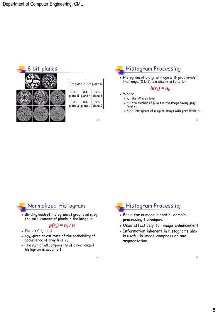
8 bit planes
Bit-plane 7 Bit-plane 6
Bit-plane 5
Bit-plane 4
Bit-plane 3
Bit-plane 2
Bit-plane 1
Bit-plane 0
30
Histogram Processing
Histogram of a digital image with gray levels in the range [0,L-1] is a discrete function
h(rk) = nk Where
rk : the kth gray level
nk : the number of pixels in the image having gray level rk
h(rk) : histogram of a digital image with gray levels rk
31
Normalized Histogram
dividing each of histogram at gray level rk by the total number of pixels in the image, n
p(rk) = nk / n For k = 0,1,…,L-1
p(rk) gives an estimate of the probability of occurrence of gray level rk
The sum of all components of a normalized histogram is equal to 1
32
Histogram Processing
Basic for numerous spatial domain processing techniques
Used effectively for image enhancement
Information inherent in histograms also is useful in image compression and segmentation
Department of Computer Engineering, CMU
9
33
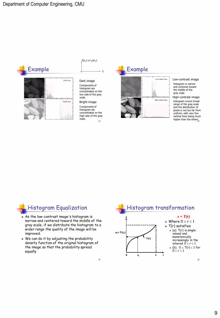
Example rk
h(rk) or p(rk)
Dark image
Bright image
Components of histogram are concentrated on the
low side of the gray scale.
Components of histogram are concentrated on the
high side of the gray scale.
34
Example
Low-contrast image
High-contrast image
histogram is narrow and centered toward the middle of the
gray scale
histogram covers broad range of the gray scale and the distribution of
pixels is not too far from uniform, with very few vertical lines being much
higher than the others
35
Histogram Equalization
As the low-contrast image’s histogram is narrow and centered toward the middle of the gray scale, if we distribute the histogram to a wider range the quality of the image will be improved.
We can do it by adjusting the probability density function of the original histogram of the image so that the probability spread equally
36
0 1 rk
sk= T(rk)
s
r
T(r)
Histogram transformation
s = T(r)
Where 0 r 1 T(r) satisfies
(a). T(r) is single-valued and monotonically increasingly in the interval 0 r 1
(b). 0 T(r) 1 for 0 r 1
Department of Computer Engineering, CMU
10
37
2 Conditions of T(r)
Single-valued (one-to-one relationship) guarantees that the inverse transformation will exist
Monotonicity condition preserves the increasing order from black to white in the output image
0 T(r) 1 for 0 r 1 guarantees that the output gray levels will be in the same range as the input levels.
The inverse transformation from s back to r is
r = T -1(s) ; 0 s 1 38
Probability Density Function
The gray levels in an image may be viewed as random variables in the interval [0,1]
PDF is one of the fundamental descriptors of a random variable
39
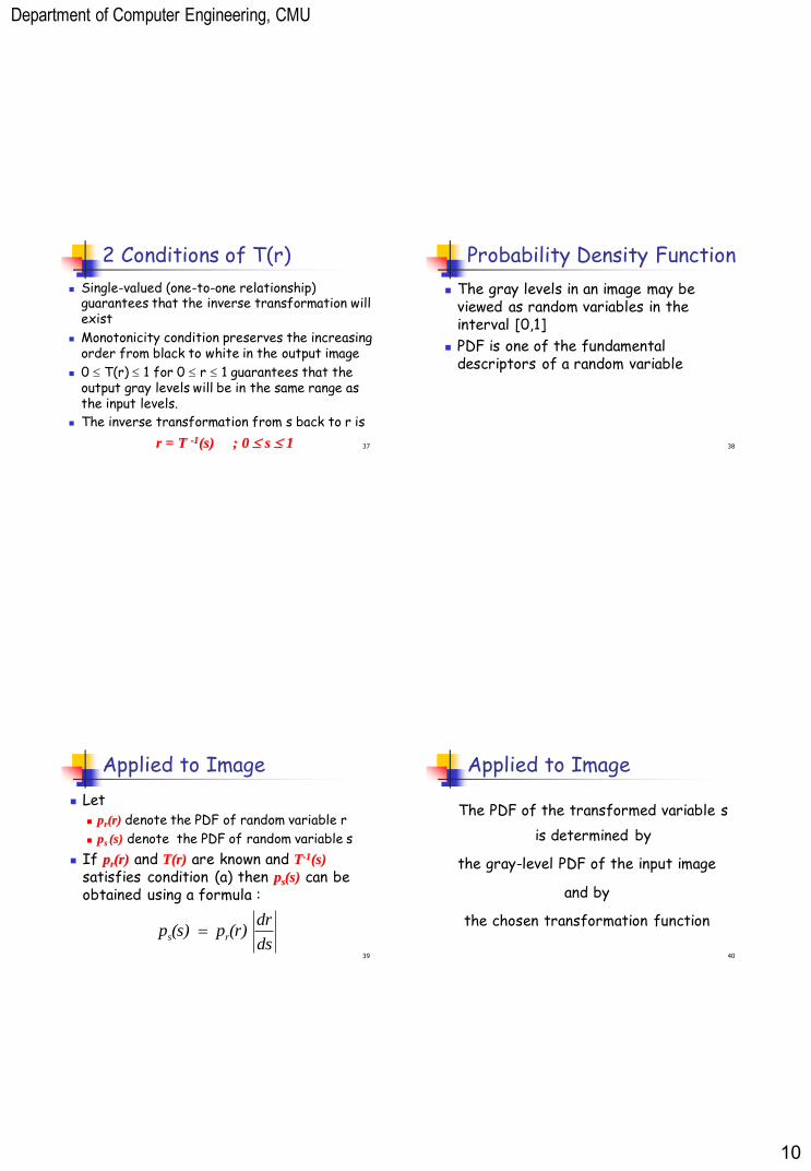
Applied to Image
Let pr(r) denote the PDF of random variable r
ps (s) denote the PDF of random variable s
If pr(r) and T(r) are known and T-1(s) satisfies condition (a) then ps(s) can be obtained using a formula :
ds
dr(r) p(s) p rs
40
Applied to Image
The PDF of the transformed variable s
is determined by
the gray-level PDF of the input image
and by
the chosen transformation function
Department of Computer Engineering, CMU
11
41
r
r dw)w(p)r(Ts0
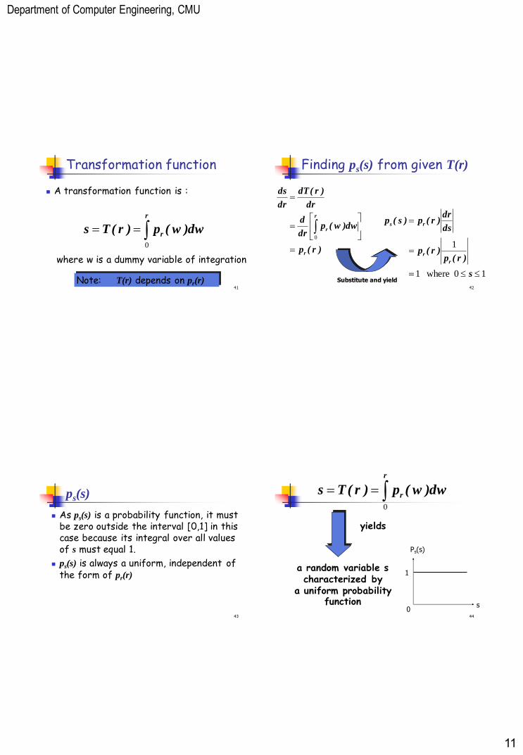
Transformation function
A transformation function is :
where w is a dummy variable of integration
Note: T(r) depends on pr(r) 42
Finding ps(s) from given T(r)
)r(p
dw)w(pdr
d
dr
)r(dT
dr
ds
r
r
r
0
10 where1
1
s
)r(p)r(p
ds
dr)r(p)s(p
r
r
rs
Substitute and yield
43
ps(s)
As ps(s) is a probability function, it must be zero outside the interval [0,1] in this case because its integral over all values of s must equal 1.
ps(s) is always a uniform, independent of the form of pr(r)
44
r
r dw)w(p)r(Ts0
a random variable s characterized by
a uniform probability function
yields
0
1
s
Ps(s)
Department of Computer Engineering, CMU
12
45
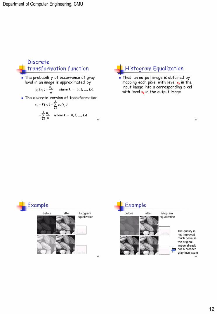
Discrete transformation function
The probability of occurrence of gray level in an image is approximated by
The discrete version of transformation
k
j
j
k
j
jrkk
, ..., L-, where kn
n
)r(p)r(Ts
0
0
110
110 , ..., L-, where k n
n)r(p k
kr
46
Histogram Equalization
Thus, an output image is obtained by mapping each pixel with level rk in the input image into a corresponding pixel with level sk in the output image
47
Example
before after Histogram
equalization
48
Example
before after Histogram
equalization
The quality is
not improved much because
the original
image already has a broaden
gray-level scale
Department of Computer Engineering, CMU
13
49
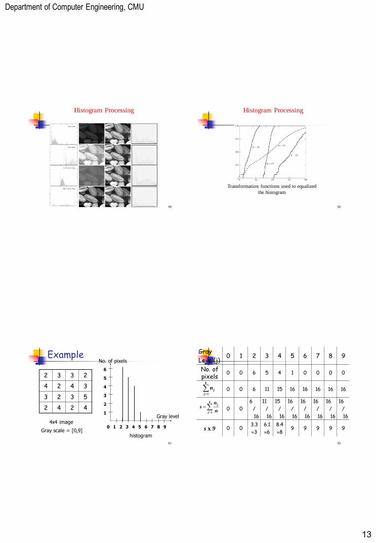
Histogram Processing
50
Histogram Processing
Transformation functions used to equalized
the histogram
51
Example
2 3 3 2
4 2 4 3
3 2 3 5
2 4 2 4
4x4 image
Gray scale = [0,9] histogram
0 1
1
2
2
3
3
4
4
5
5
6
6
7 8 9
No. of pixels
Gray level
52
Gray
Level(j) 0 1 2 3 4 5 6 7 8 9
No. of pixels
0 0 6 5 4 1 0 0 0 0
0 0 6 11 15 16 16 16 16 16
0 0
6
/
16
11
/
16
15
/
16
16
/
16
16
/
16
16
/
16
16
/
16
16
/
16
s x 9 0 0 3.3
3
6.1
6
8.4
8 9 9 9 9 9
k
j
jn0
k
j
j
n
ns
0
Department of Computer Engineering, CMU
14
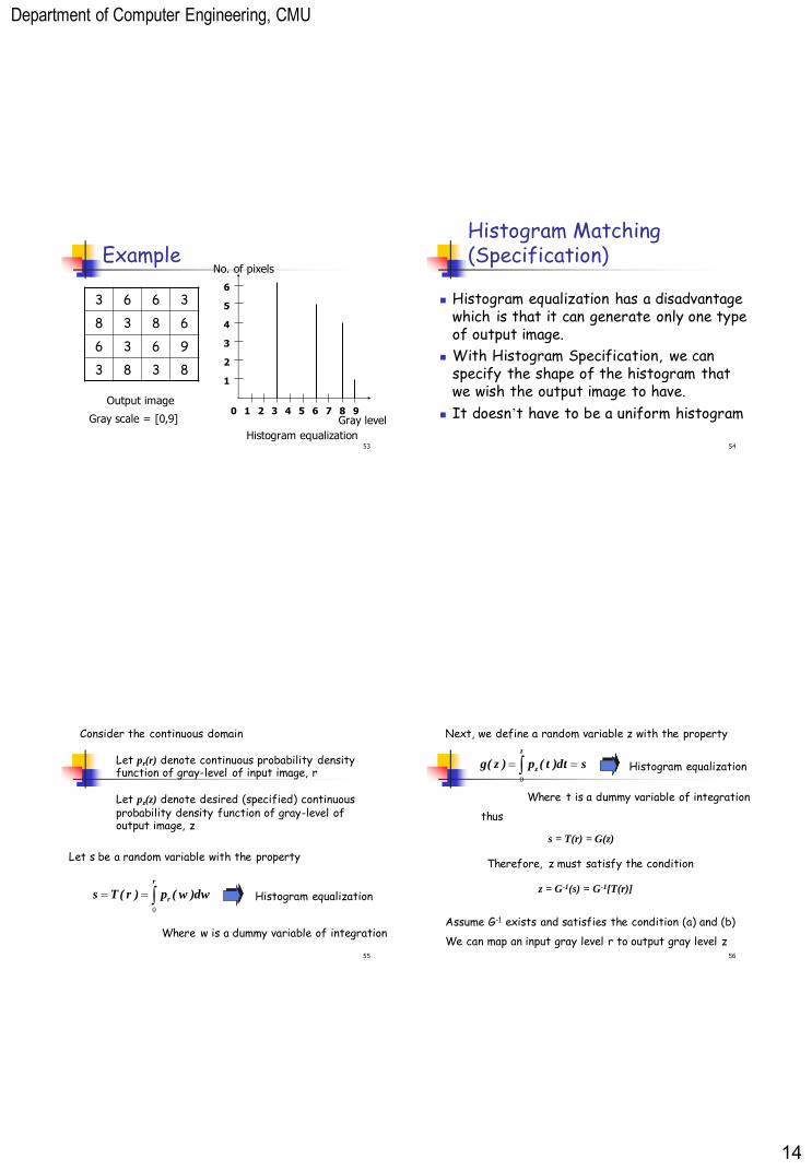
53
Example
3 6 6 3
8 3 8 6
6 3 6 9
3 8 3 8
Output image
Gray scale = [0,9]
Histogram equalization
0 1
1
2
2
3
3
4
4
5
5
6
6
7 8 9
No. of pixels
Gray level
54
Histogram Matching (Specification)
Histogram equalization has a disadvantage which is that it can generate only one type of output image.
With Histogram Specification, we can specify the shape of the histogram that we wish the output image to have.
It doesn’t have to be a uniform histogram
55
Consider the continuous domain
Let pr(r) denote continuous probability density function of gray-level of input image, r
Let pz(z) denote desired (specified) continuous probability density function of gray-level of output image, z
Let s be a random variable with the property
r
r dw)w(p)r(Ts0
Where w is a dummy variable of integration
Histogram equalization
56
Next, we define a random variable z with the property
s = T(r) = G(z)
We can map an input gray level r to output gray level z
thus
sdt)t(p)z(g
z
z 0
Where t is a dummy variable of integration
Histogram equalization
Therefore, z must satisfy the condition
z = G-1(s) = G-1[T(r)]
Assume G-1 exists and satisfies the condition (a) and (b)
Department of Computer Engineering, CMU
15
57
Histogram Processing
Histogram Matching (Specification)
58
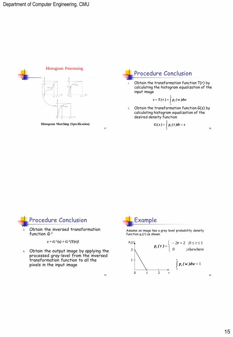
Procedure Conclusion
1. Obtain the transformation function T(r) by calculating the histogram equalization of the input image
2. Obtain the transformation function G(z) by calculating histogram equalization of the desired density function
r
r dw)w(p)r(Ts0
sdt)t(p)z(G
z
z 0
59
Procedure Conclusion
3. Obtain the inversed transformation function G-1
4. Obtain the output image by applying the processed gray-level from the inversed transformation function to all the pixels in the input image
z = G-1(s) = G-1[T(r)]
60
Example
Assume an image has a gray level probability density function pr(r) as shown.
0 1 2
1
2
Pr(r)
elsewhere; 0
1r;0 22r)r(pr
10
r
r dw)w(p
r
Department of Computer Engineering, CMU
16
61
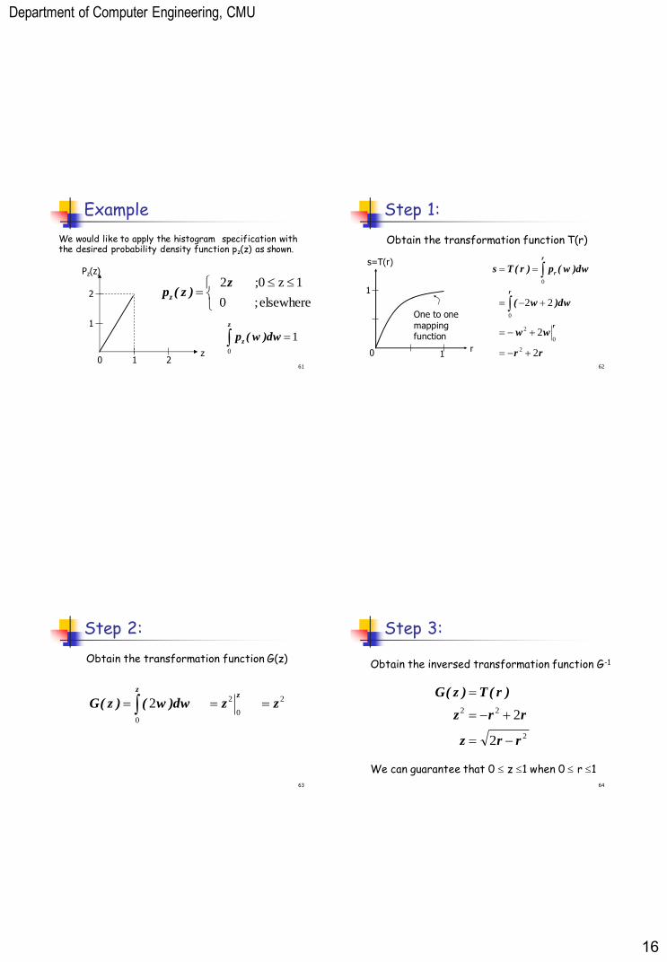
Example
We would like to apply the histogram specification with the desired probability density function pz(z) as shown.
0 1 2
1
2
Pz(z)
z
elsewhere; 0
1z;0 2z)z(pz
10
z
z dw)w(p
62
Step 1:
0 1
1
s=T(r)
r rr
ww
dw)w(
dw)w(p)r(Ts
r
r
r
r
2
2
22
2
0
2
0
0
Obtain the transformation function T(r)
One to one
mapping function
63
Step 2:
2
0
2
0
2 zzdw)w()z(Gz
z
Obtain the transformation function G(z)
64
Step 3:
2
22
2
2
rrz
rrz
)r(T)z(G
Obtain the inversed transformation function G-1
We can guarantee that 0 z 1 when 0 r 1
Department of Computer Engineering, CMU
17
65
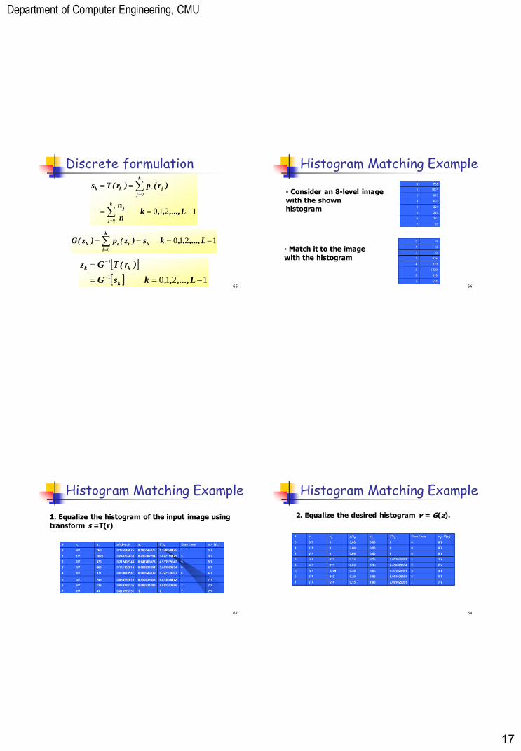
Discrete formulation
1210 0
L,...,,,ks)z(p)z(G k
k
i
izk
1210 0
0
L,...,,,kn
n
)r(p)r(Ts
k
j
j
k
j
jrkk
1210 1
1
L,...,,,ksG
)r(TGz
k
kk
66
• Consider an 8-level image
with the shown histogram
• Match it to the image
with the histogram
Histogram Matching Example
67
Histogram Matching Example
1. Equalize the histogram of the input image using
transform s =T(r)
68
Histogram Matching Example
2. Equalize the desired histogram v = G(z).
Department of Computer Engineering, CMU
18
69
Histogram Matching Example
3. Set v = s to obtain the composite
transform
70
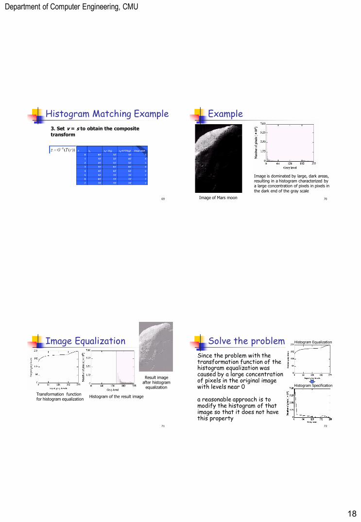
Example
Image of Mars moon
Image is dominated by large, dark areas, resulting in a histogram characterized by a large concentration of pixels in pixels in
the dark end of the gray scale
71
Image Equalization
Result image after histogram
equalization
Transformation function for histogram equalization
Histogram of the result image
72
Histogram Equalization
Histogram Specification
Solve the problem
Since the problem with the transformation function of the histogram equalization was caused by a large concentration of pixels in the original image with levels near 0
a reasonable approach is to modify the histogram of that image so that it does not have this property
Department of Computer Engineering, CMU
19
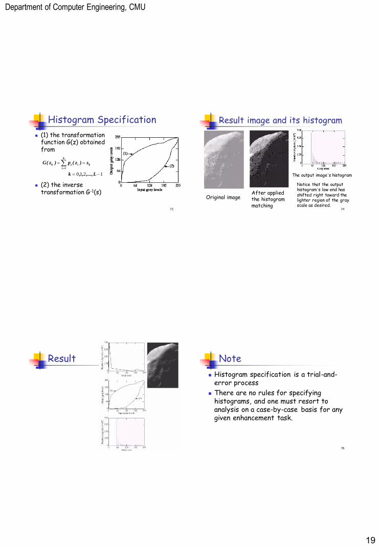
73
Histogram Specification
(1) the transformation function G(z) obtained from
(2) the inverse transformation G-1(s)
1210
0
L,...,,,k
s)z(p)z(G k
k
i
izk
74
Result image and its histogram
Original image
The output image’s histogram
Notice that the output histogram’s low end has shifted right toward the lighter region of the gray scale as desired.
After applied the histogram matching
75
Result
76
Note
Histogram specification is a trial-and-error process
There are no rules for specifying histograms, and one must resort to analysis on a case-by-case basis for any given enhancement task.
Department of Computer Engineering, CMU
20
77
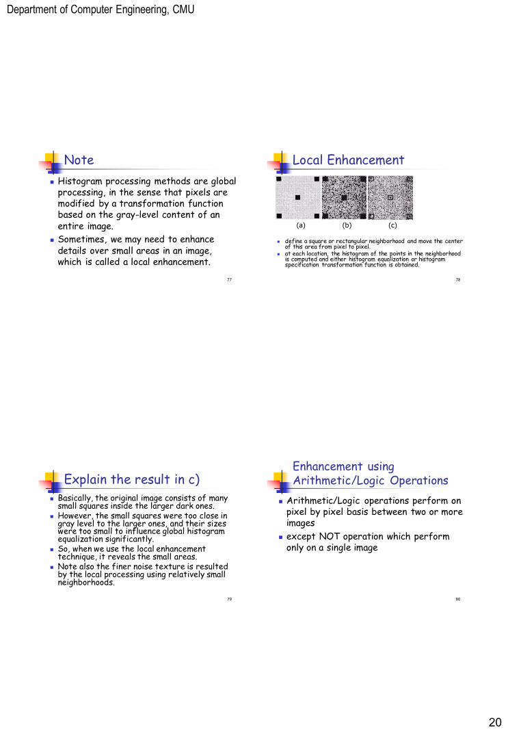
Note
Histogram processing methods are global processing, in the sense that pixels are modified by a transformation function based on the gray-level content of an entire image.
Sometimes, we may need to enhance details over small areas in an image, which is called a local enhancement.
78
Local Enhancement
define a square or rectangular neighborhood and move the center of this area from pixel to pixel.
at each location, the histogram of the points in the neighborhood is computed and either histogram equalization or histogram specification transformation function is obtained.
(a) (b) (c)
79
Explain the result in c) Basically, the original image consists of many
small squares inside the larger dark ones. However, the small squares were too close in
gray level to the larger ones, and their sizes were too small to influence global histogram equalization significantly.
So, when we use the local enhancement technique, it reveals the small areas.
Note also the finer noise texture is resulted by the local processing using relatively small neighborhoods.
80
Enhancement using Arithmetic/Logic Operations
Arithmetic/Logic operations perform on pixel by pixel basis between two or more images
except NOT operation which perform only on a single image
Department of Computer Engineering, CMU
21
81
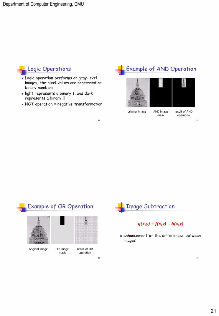
Logic Operations
Logic operation performs on gray-level images, the pixel values are processed as binary numbers
light represents a binary 1, and dark represents a binary 0
NOT operation = negative transformation
82
Example of AND Operation
original image AND image
mask
result of AND
operation
83
Example of OR Operation
original image OR image
mask
result of OR
operation
84
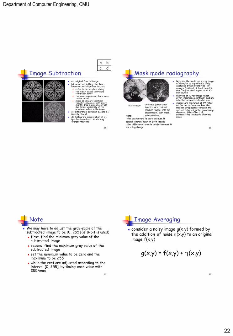
Image Subtraction
g(x,y) = f(x,y) – h(x,y)
enhancement of the differences between images
Department of Computer Engineering, CMU
22
85
Image Subtraction a). original fractal image b). result of setting the four
lower-order bit planes to zero refer to the bit-plane slicing the higher planes contribute
significant detail the lower planes contribute more
to fine detail image b). is nearly identical
visually to image a), with a very slightly drop in overall contrast due to less variability of the gray-level values in the image.
c). difference between a). and b). (nearly black)
d). histogram equalization of c). (perform contrast stretching transformation)
a b
c d
86
Mask mode radiography h(x,y) is the mask, an X-ray image
of a region of a patient’s body captured by an intensified TV camera (instead of traditional X-ray film) located opposite an X-ray source
f(x,y) is an X-ray image taken after injection a contrast medium into the patient’s bloodstream
images are captured at TV rates, so the doctor can see how the medium propagates through the various arteries in the area being observed (the effect of subtraction) in a movie showing mode.
mask image an image (taken after injection of a contrast medium (iodine) into the bloodstream) with mask
subtracted out. Note: • the background is dark because it doesn’t change much in both images. • the difference area is bright because it has a big change
87
Note
We may have to adjust the gray-scale of the subtracted image to be [0, 255] (if 8-bit is used) first, find the minimum gray value of the
subtracted image second, find the maximum gray value of the
subtracted image set the minimum value to be zero and the
maximum to be 255 while the rest are adjusted according to the
interval [0, 255], by timing each value with 255/max
88
Image Averaging
consider a noisy image g(x,y) formed by the addition of noise (x,y) to an original image f(x,y)
g(x,y) = f(x,y) + (x,y)
Department of Computer Engineering, CMU
23
89
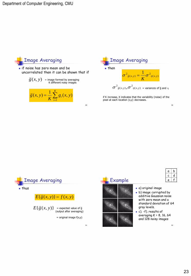
Image Averaging
if noise has zero mean and be uncorrelated then it can be shown that if
),( yxg = image formed by averaging K different noisy images
K
i
i yxgK
yxg1
),(1
),(
90
Image Averaging
then
),(2
),(2 1
yxyxg
K
= variances of g and ),(2
),(2 , yxyxg
if K increase, it indicates that the variability (noise) of the pixel at each location (x,y) decreases.
91
Image Averaging
thus
),()},({ yxfyxgE
)},({ yxgE = expected value of g
(output after averaging)
= original image f(x,y)
92
Example
a) original image
b) image corrupted by additive Gaussian noise with zero mean and a standard deviation of 64 gray levels.
c). -f). results of averaging K = 8, 16, 64 and 128 noisy images
a b
c d
e f
Department of Computer Engineering, CMU
24
93
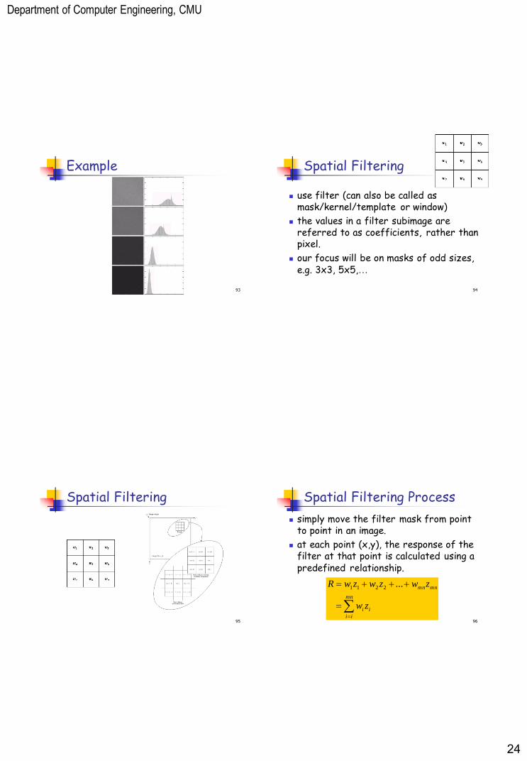
Example
94
Spatial Filtering
use filter (can also be called as mask/kernel/template or window)
the values in a filter subimage are referred to as coefficients, rather than pixel.
our focus will be on masks of odd sizes, e.g. 3x3, 5x5,…
95
Spatial Filtering
96
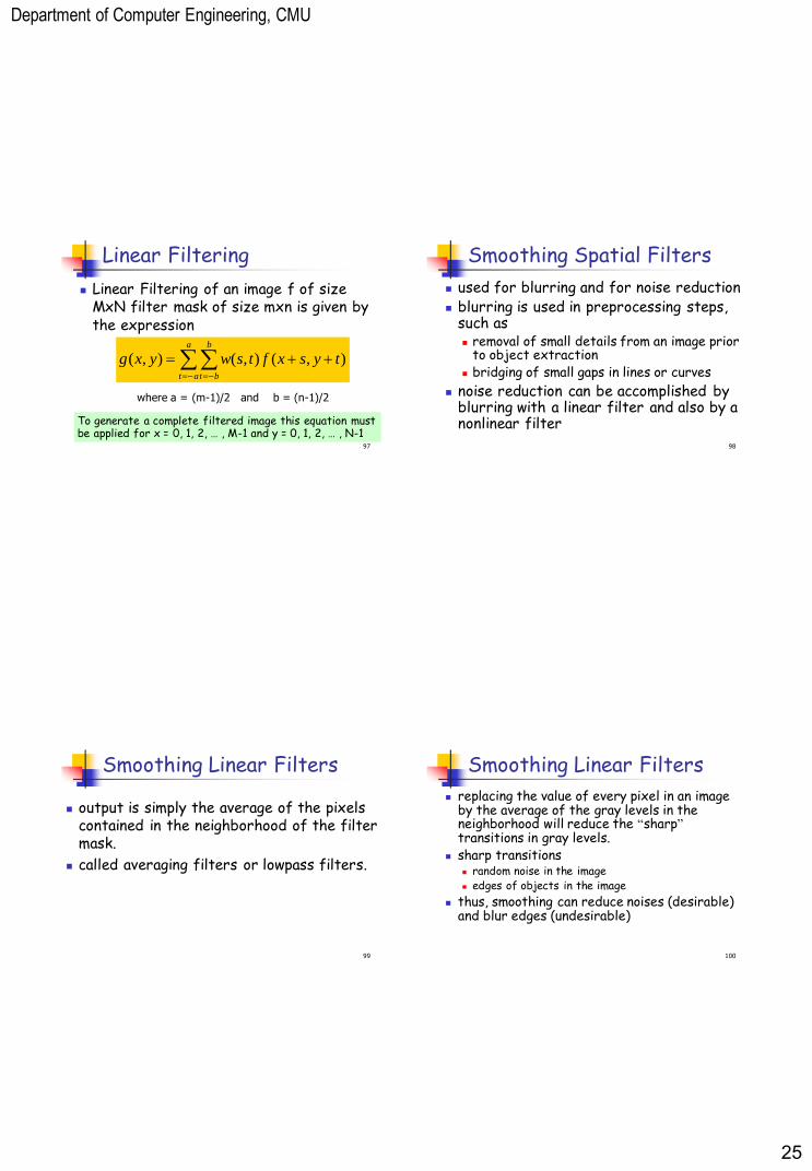
Spatial Filtering Process
simply move the filter mask from point to point in an image.
at each point (x,y), the response of the filter at that point is calculated using a predefined relationship.
mn
ii
ii
mnmn
zw
zwzwzwR ...2211
Department of Computer Engineering, CMU
25
97
Linear Filtering
Linear Filtering of an image f of size MxN filter mask of size mxn is given by the expression
a
at
b
bt
tysxftswyxg ),(),(),(
where a = (m-1)/2 and b = (n-1)/2
To generate a complete filtered image this equation must be applied for x = 0, 1, 2, … , M-1 and y = 0, 1, 2, … , N-1
98
Smoothing Spatial Filters
used for blurring and for noise reduction blurring is used in preprocessing steps,
such as removal of small details from an image prior
to object extraction bridging of small gaps in lines or curves
noise reduction can be accomplished by blurring with a linear filter and also by a nonlinear filter
99
Smoothing Linear Filters
output is simply the average of the pixels contained in the neighborhood of the filter mask.
called averaging filters or lowpass filters.
100
Smoothing Linear Filters
replacing the value of every pixel in an image by the average of the gray levels in the neighborhood will reduce the “sharp” transitions in gray levels.
sharp transitions random noise in the image edges of objects in the image
thus, smoothing can reduce noises (desirable) and blur edges (undesirable)
Department of Computer Engineering, CMU
26
101
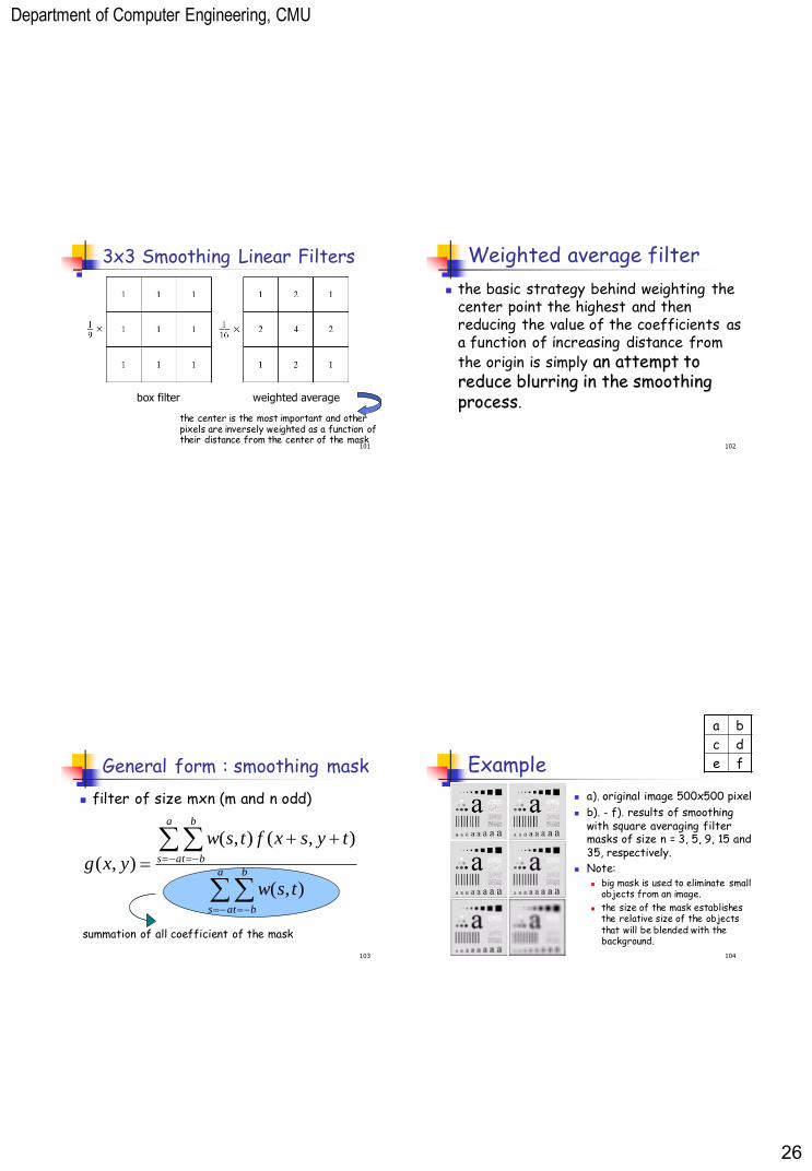
3x3 Smoothing Linear Filters
box filter weighted average
the center is the most important and other pixels are inversely weighted as a function of their distance from the center of the mask
102
Weighted average filter
the basic strategy behind weighting the center point the highest and then reducing the value of the coefficients as a function of increasing distance from the origin is simply an attempt to reduce blurring in the smoothing process.
103
General form : smoothing mask
filter of size mxn (m and n odd)
a
as
b
bt
a
as
b
bt
tsw
tysxftsw
yxg
),(
),(),(
),(
summation of all coefficient of the mask
104
Example
a). original image 500x500 pixel
b). - f). results of smoothing with square averaging filter masks of size n = 3, 5, 9, 15 and 35, respectively.
Note: big mask is used to eliminate small
objects from an image.
the size of the mask establishes the relative size of the objects that will be blended with the background.
a b
c d
e f
Department of Computer Engineering, CMU
27
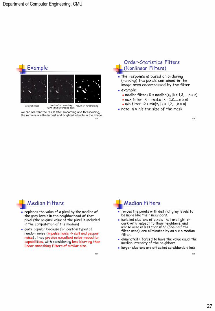
105
Example
original image result after smoothing with 15x15 averaging mask
result of thresholding
we can see that the result after smoothing and thresholding, the remains are the largest and brightest objects in the image.
106
Order-Statistics Filters (Nonlinear Filters)
the response is based on ordering (ranking) the pixels contained in the image area encompassed by the filter
example median filter : R = median{zk |k = 1,2,…,n x n} max filter : R = max{zk |k = 1,2,…,n x n} min filter : R = min{zk |k = 1,2,…,n x n}
note: n x nis the size of the mask
107
Median Filters
replaces the value of a pixel by the median of the gray levels in the neighborhood of that pixel (the original value of the pixel is included in the computation of the median)
quite popular because for certain types of random noise (impulse noise salt and pepper noise) , they provide excellent noise-reduction capabilities, with considering less blurring than linear smoothing filters of similar size.
108
Median Filters
forces the points with distinct gray levels to be more like their neighbors.
isolated clusters of pixels that are light or dark with respect to their neighbors, and whose area is less than n2/2 (one-half the filter area), are eliminated by an n x n median filter.
eliminated = forced to have the value equal the median intensity of the neighbors.
larger clusters are affected considerably less
Department of Computer Engineering, CMU
28
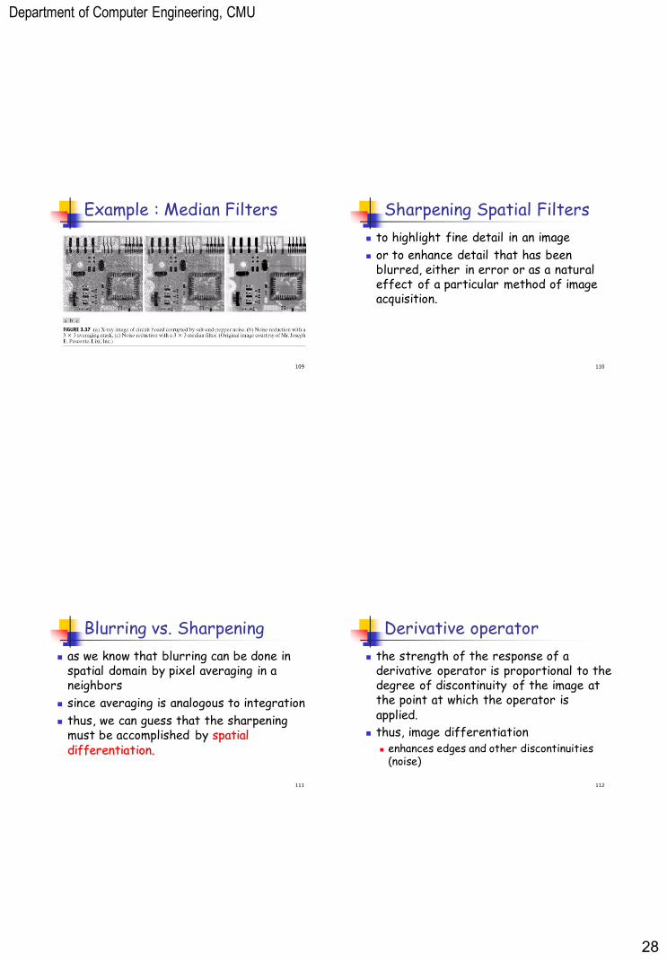
109
Example : Median Filters
110
Sharpening Spatial Filters
to highlight fine detail in an image
or to enhance detail that has been blurred, either in error or as a natural effect of a particular method of image acquisition.
111
Blurring vs. Sharpening
as we know that blurring can be done in spatial domain by pixel averaging in a neighbors
since averaging is analogous to integration
thus, we can guess that the sharpening must be accomplished by spatial differentiation.
112
Derivative operator
the strength of the response of a derivative operator is proportional to the degree of discontinuity of the image at the point at which the operator is applied.
thus, image differentiation enhances edges and other discontinuities
(noise)
Department of Computer Engineering, CMU
29
113
First-order derivative
a basic definition of the first-order derivative of a one-dimensional function f(x) is the difference
)()1( xfxfx
f
114
Second-order derivative
similarly, we define the second-order derivative of a one-dimensional function f(x) is the difference
)(2)1()1(2
2
xfxfxfx
f
115
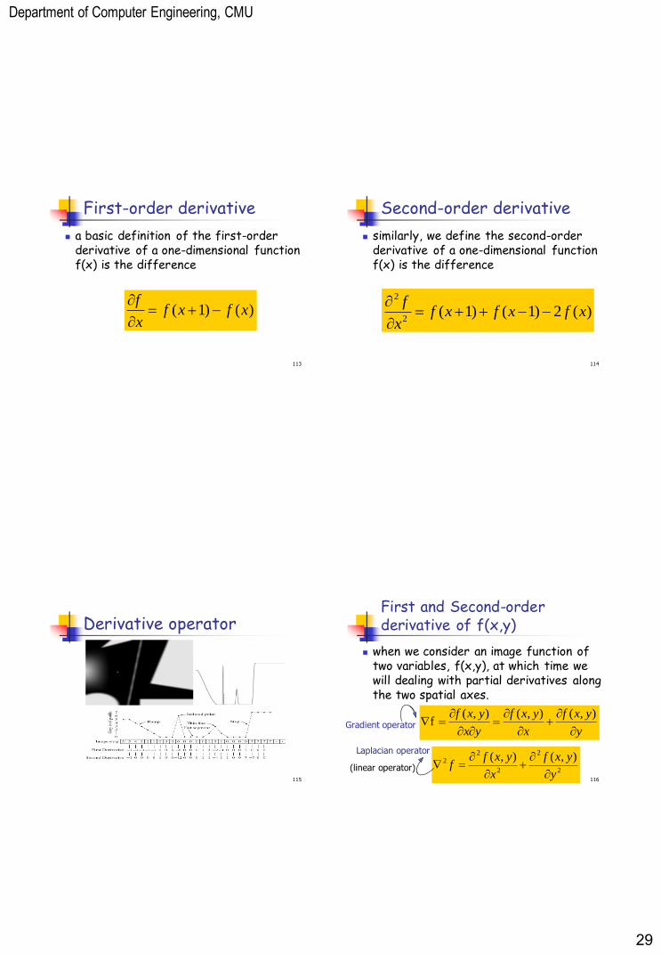
Derivative operator
116
First and Second-order derivative of f(x,y)
when we consider an image function of two variables, f(x,y), at which time we will dealing with partial derivatives along the two spatial axes.
y
yxf
x
yxf
yx
yxf
),(),(),(f
2
2
2
22 ),(),(
y
yxf
x
yxff
(linear operator)
Laplacian operator
Gradient operator
Department of Computer Engineering, CMU
30
117
Discrete Form of Laplacian
),(2),1(),1(2
2
yxfyxfyxfx
f
),(2)1,()1,(2
2
yxfyxfyxfy
f
from
yield,
)],(4)1,()1,(
),1(),1([2
yxfyxfyxf
yxfyxff
118
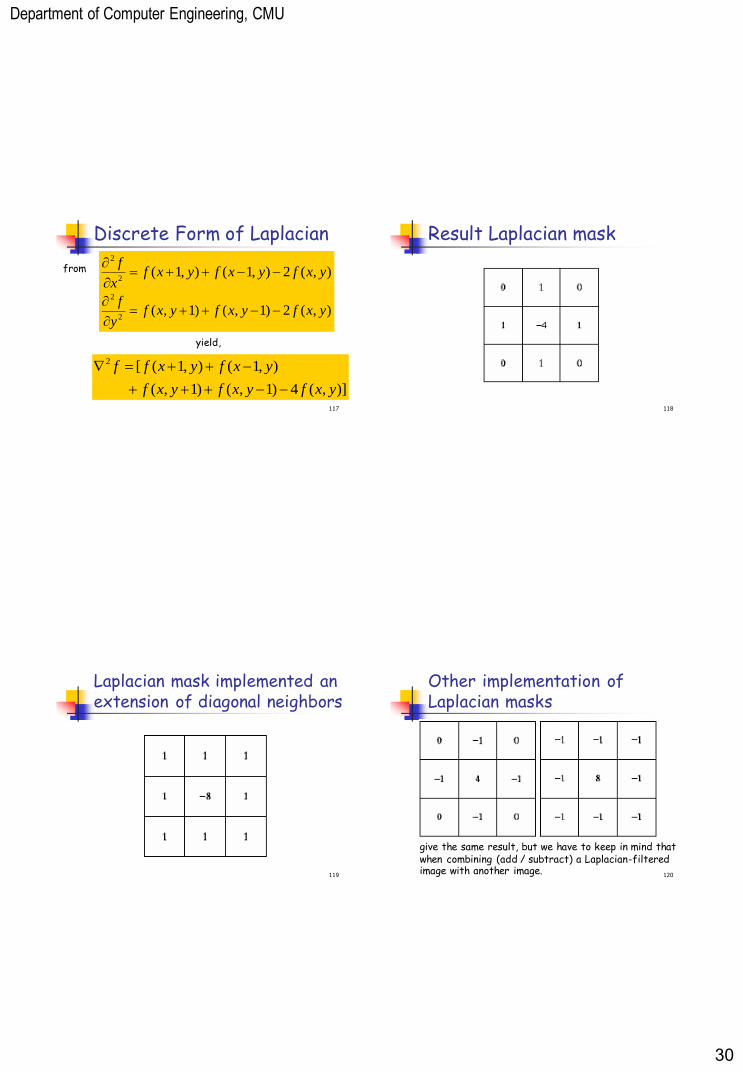
Result Laplacian mask
119
Laplacian mask implemented an extension of diagonal neighbors
120
Other implementation of Laplacian masks
give the same result, but we have to keep in mind that when combining (add / subtract) a Laplacian-filtered image with another image.
Department of Computer Engineering, CMU
31
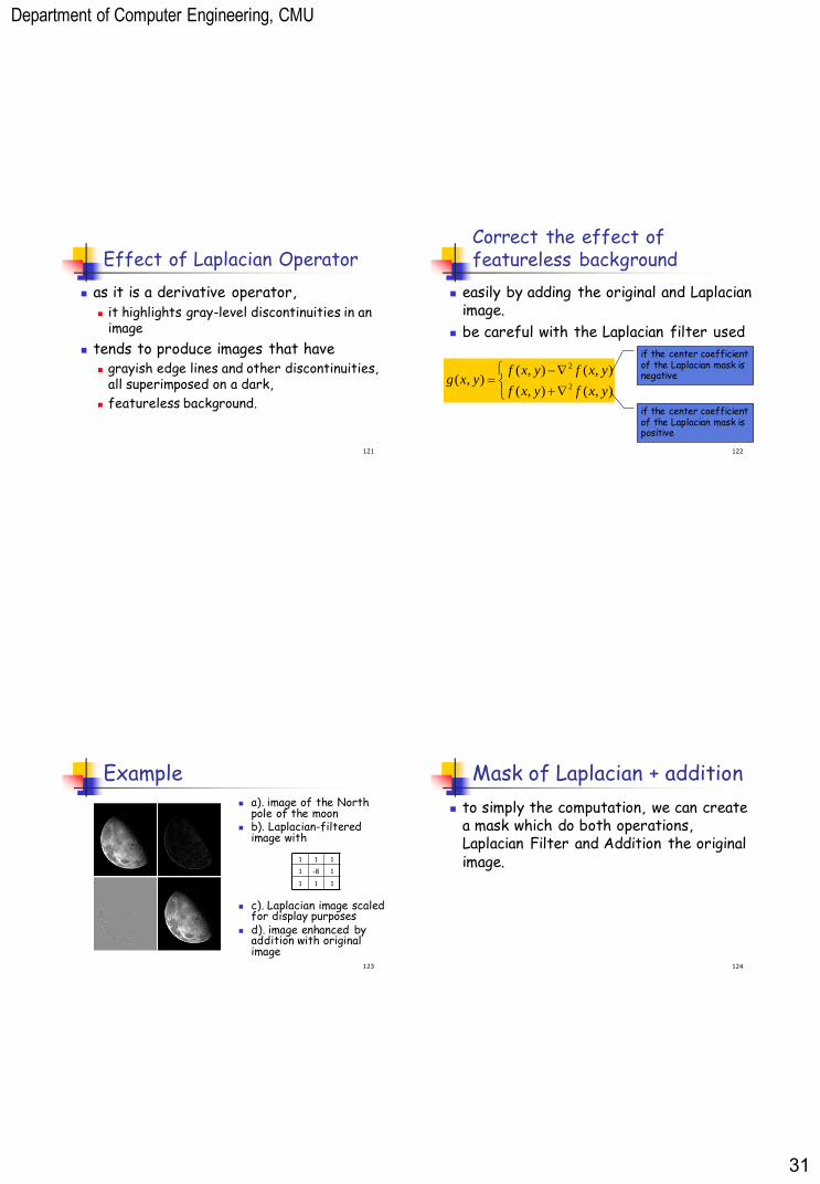
121
Effect of Laplacian Operator
as it is a derivative operator, it highlights gray-level discontinuities in an
image
tends to produce images that have grayish edge lines and other discontinuities,
all superimposed on a dark,
featureless background.
122
Correct the effect of featureless background
easily by adding the original and Laplacian image.
be careful with the Laplacian filter used
),(),(
),(),(),(
2
2
yxfyxf
yxfyxfyxg
if the center coefficient of the Laplacian mask is negative
if the center coefficient of the Laplacian mask is positive
123
Example
a). image of the North pole of the moon
b). Laplacian-filtered image with
c). Laplacian image scaled for display purposes
d). image enhanced by addition with original image
1 1 1
1 -8 1
1 1 1
124
Mask of Laplacian + addition
to simply the computation, we can create a mask which do both operations, Laplacian Filter and Addition the original image.
Department of Computer Engineering, CMU
32
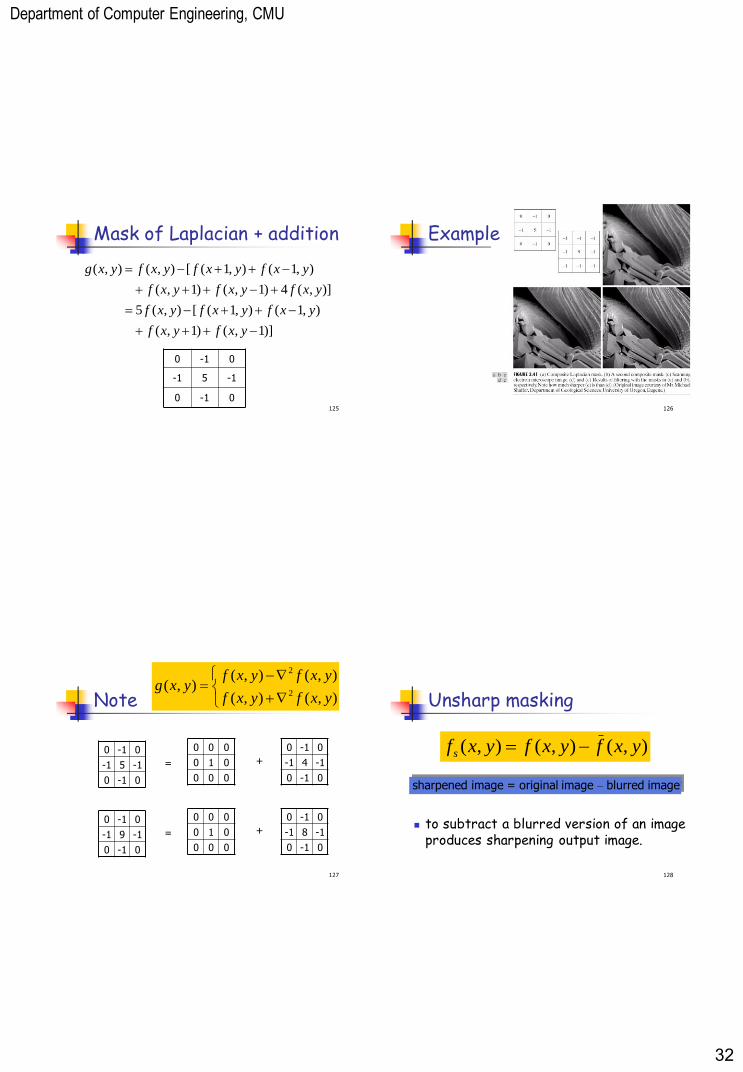
125
Mask of Laplacian + addition
)]1,()1,(
),1(),1([),(5
)],(4)1,()1,(
),1(),1([),(),(
yxfyxf
yxfyxfyxf
yxfyxfyxf
yxfyxfyxfyxg
0 -1 0
-1 5 -1
0 -1 0 126
Example
127
Note
0 -1 0
-1 5 -1
0 -1 0
0 0 0
0 1 0
0 0 0
),(),(
),(),(),(
2
2
yxfyxf
yxfyxfyxg
= + 0 -1 0
-1 4 -1
0 -1 0
0 -1 0
-1 9 -1
0 -1 0
0 0 0
0 1 0
0 0 0
= + 0 -1 0
-1 8 -1
0 -1 0
128
Unsharp masking
to subtract a blurred version of an image produces sharpening output image.
),(),(),( yxfyxfyxfs
sharpened image = original image – blurred image
Department of Computer Engineering, CMU
33
129
High-boost filtering
generalized form of Unsharp masking A 1
130
High-boost filtering
if we use Laplacian filter to create sharpen image fs(x,y) with addition of original image
),(),(
),(),(),(
2
2
yxfyxf
yxfyxfyxf s
131
High-boost filtering
yields
),(),(
),(),(),(
2
2
yxfyxAf
yxfyxAfyxfhb
if the center coefficient of the Laplacian mask is negative
if the center coefficient of the Laplacian mask is positive
132
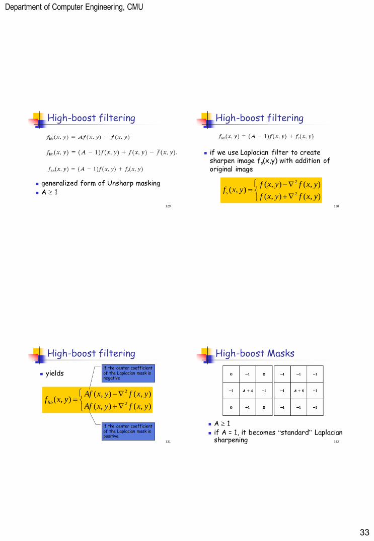
High-boost Masks
A 1 if A = 1, it becomes “standard” Laplacian
sharpening
Department of Computer Engineering, CMU
34
133
Example
134
Gradient Operator
first derivatives are implemented using the magnitude of the gradient.
y
fx
f
G
G
y
xf
21
22
21
22 ][)f(
y
f
x
f
GGmagf yx
the magnitude becomes nonlinear yx GGf
commonly approx.
135
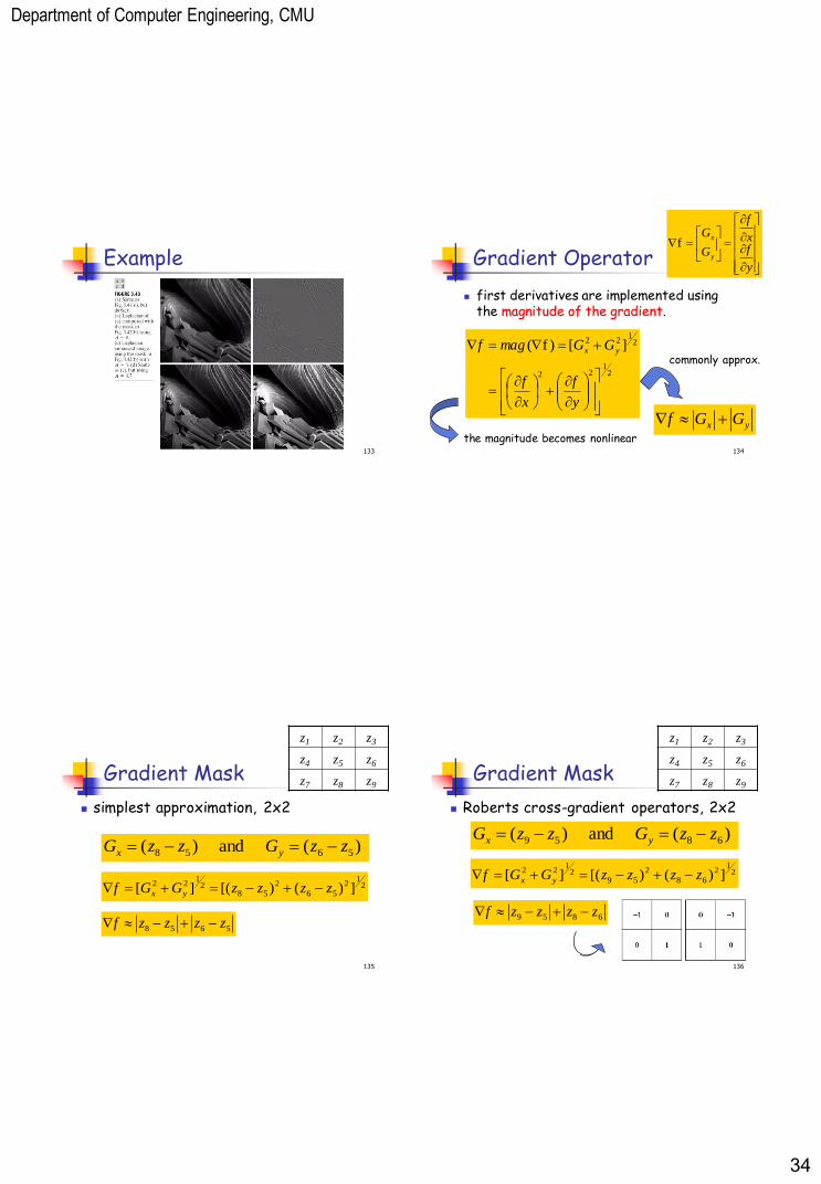
Gradient Mask
simplest approximation, 2x2
z1 z2 z3
z4 z5 z6
z7 z8 z9
)( and )( 5658 zzGzzG yx
21
2
56
2
582
122 ])()[(][ zzzzGGf yx
5658 zzzzf
136
Gradient Mask
Roberts cross-gradient operators, 2x2
z1 z2 z3
z4 z5 z6
z7 z8 z9
)( and )( 6859 zzGzzG yx
21
2
68
2
592
122 ])()[(][ zzzzGGf yx
6859 zzzzf
Department of Computer Engineering, CMU
35
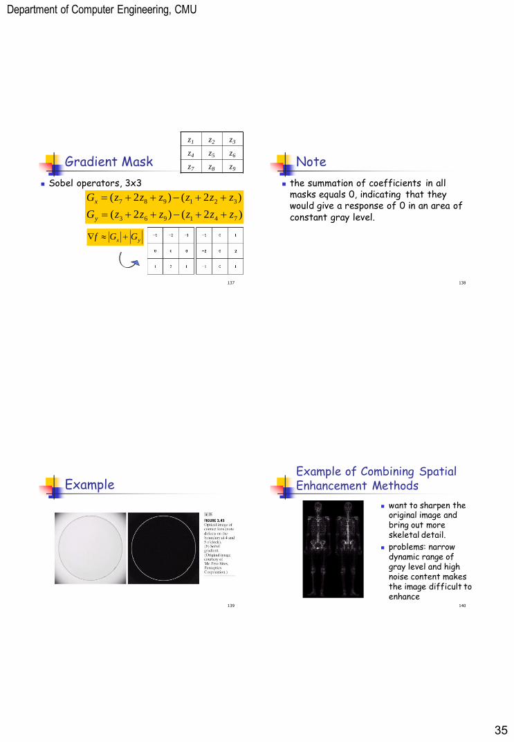
137
Gradient Mask
Sobel operators, 3x3
z1 z2 z3
z4 z5 z6
z7 z8 z9
)2()2(
)2()2(
741963
321987
zzzzzzG
zzzzzzG
y
x
yx GGf
138
Note
the summation of coefficients in all masks equals 0, indicating that they would give a response of 0 in an area of constant gray level.
139
Example
140
Example of Combining Spatial Enhancement Methods
want to sharpen the original image and bring out more skeletal detail.
problems: narrow dynamic range of gray level and high noise content makes the image difficult to enhance
Department of Computer Engineering, CMU
36
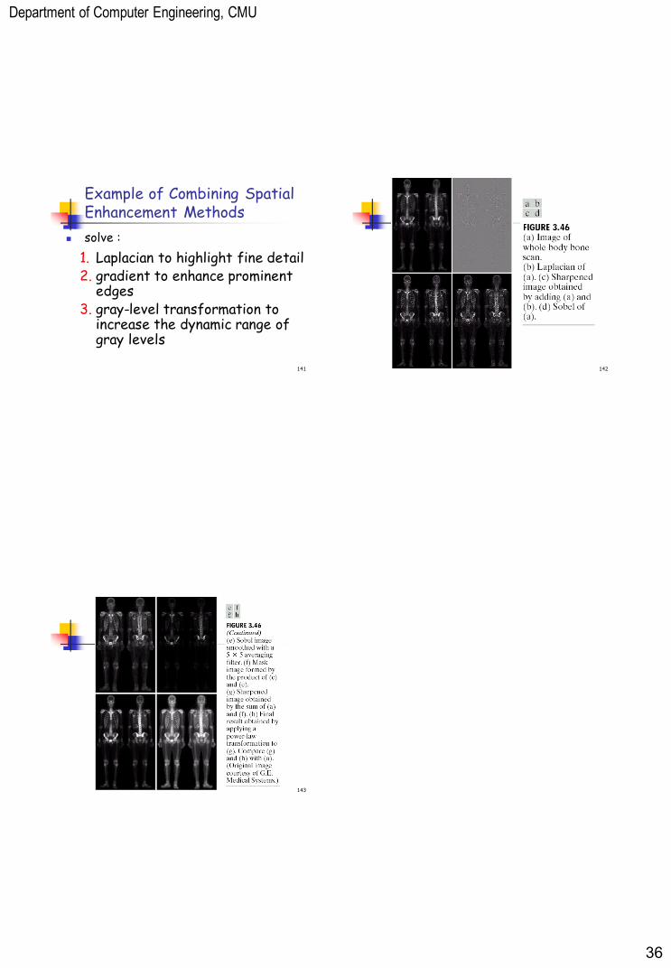
141
Example of Combining Spatial Enhancement Methods
solve : 1. Laplacian to highlight fine detail 2. gradient to enhance prominent
edges 3. gray-level transformation to
increase the dynamic range of gray levels
142
143