Dimensions required to estimate the rainfall in a region

8/7/2019 Dimensions required to estimate the rainfall in a region

http://slidepdf.com/reader/full/dimensions-required-to-estimate-the-rainfall-in-a-region 1/30

A

B.Tech. Credit Project Report

On

Chaos Theory In Hydrology

Submitted by

Nirdesh Kumar

Roll No-06004008

Under the Supervision of

Prof. V Jothiprakash

Department of Civil Engineering

Indian Institute of Technology, Bombay

Mumbai – 400 076, India.

Nov. 2009

i



Approval Certificate

The B.Tech. Credit Project (CE 497) report entitled ‘Chaos Theory In Hydrology’ by

Nirdesh Kumar (Roll No-06004008) can be considered for evaluation.

Date:6/11/09 Supervisor

IIT BOMBAY Prof. V Jothiprakash

ii



Acknowledgement

I express my sincere thanks and humble appreciation to Prof. V Jothiprakash, Department of

Civil Engineering, IIT BOMBAY, for his inspiring suggestions, whole hearted co-operation,

constructive criticism and continuous encouragement in the preparation of this credit Project

report, without which it would not have been in its present shape.

I would also like to convey my thanks to the Department of Civil Engineering for providing

me the necessary facilities.

Nirdesh Kumar

Roll No-06004008

iii



Abstract

The main aim of the study is to estimate the number of dependable dimensions to predict the

rainfall in a region using Chaos Theory.

The correlation dimension method is employed to identify the behaviour of rainfall dynamics,

and investigate the existence of chaotic behaviour in the rainfall data of koyna dam over a

period of 47 years.

Rainfall data for 12 different temporal scales is analysed and the correlation dimension i used

as a basis for discriminating stochastic and chaotic behaviours.

iv



Content Page No.

Chapter 1 Introduction 1

1.1Deterministic, Stochastic and Chaotic systems 1

1.2Chaos Identification Methods 2

1.3 Objectives Of The Study 2

1.4 Organisation Of Chapters 2

Chapter 2 Chaos Theory In Hydrology 4

2.1 Introduction 4

2.2 Limitations Of Data 4

2.3 Data Size and Sampling Frequency 5

2.4 Noise 5

2.5 Delay Time 6

2.6 Correlation Dimension Algorithm 6

2.7 Summary 8

Chapter 3 Chaos In Koyna Dam Rainfall 9

3.1 Description Of The Study Region 9

3.2 Data Analysis 9

3.3 Results 25

Chapter 4 Conclusion 27

References 28

List Of Figures

Figure 1: Koyna Dam 9

Figure 2: Variation of rainfall series at Koyna Dam 10Figure 3: Auto-correlation function for different rainfall series 14

Figure 4: Phase-space reconstruction for different rainfall series 20

Figure 5: Log C(r) versus Log r plot for different rainfall series 21

Figure 6: Relationship between correlation exponent and embedding dimension 25

v



Chapter 1

Introduction

1.1 Deterministic, Stochastic and Chaotic systems

During the past few decades, a number of mathematical models have been proposed for

modeling hydrological processes.However, due to considerable spatial and temporal

variability, and limitation in the availability of appropriate mathematical tools, no unified

mathematical approach has been established.

Untill recently, the tremendous spatial and temporal variability of hydrological processes has

been believed to be due to the influence of a large number of variables. Consequently, the

majority of the previous investigations on modeling hydrological processes have essentially

employed the concept of a stochastic process. However, recent studies have indicated that

even simple deterministic systems, influenced by a few nonlinear interdependent variables,

might give rise to ‘deterministic chaos’.Hence, it is now believed that the dynamic structures

of complex hydrological processes, such as rainfall and runoff, can be better understood

using nonlinear deterministic chaotic models than the stochastic ones.

A system is said to be deterministic if knowledge of the time-evolutions, the parameters that

describe the system, and the initial conditions in principle completely determine the

subsequent behavior of the system. Hence for deterministic systems, long-term prediction is

feasible. In stochastic systems, the input parameters are, in general, unknown or only some

statistical measures of the parameters are known. For such systems, even short-term

predictability is not guaranteed.

The term "chaos" in the chaotic system is used to denote the irregular behavior of dynamical

systems arising from a strictly deterministic time evolution without any source of noise or

external stochasticity but with sensitivity to initial conditions, which means small

perturbations in the initial conditions will have large effects in the future.

Complex processes often require a large number of variables and equations to satisfactorily

represent and model them.The study of Chaos helps us to identify the minimum number of

variables essential and the number of variables sufficient to model the dynamics of the

systems.

1



1.2 Chaos Identification methods

The available methods to investigate the existence of chaos in a time series are still in the

state of infancy. Though a wide variety of methods are available, such as the correlation

dimension method (e.g. Grassberger and Procaccia, 1983a), the Lyapunov exponent method

(e.g. Wolf et al., 1985), the Kolmogorov entropy method (e.g. Grassberger and Procaccia,

1983b), the nonlinear prediction method (e.g. Farmer ; Casdagli; Casdagli and Sugihara), and

the surrogate data method (e.g. Theiler ; Theiler and Schreiber ), there is no single method that

can provide an infallible distinction between a chaotic and a stochastic system. For instance:

(1) a finite correlation dimension, usually understood as the principal, if not unique, sign of

deterministic chaos, may be observed also for a stochastic process (e.g. Osborne and

Provenzale, 1989); (2) an autoregressive (AR) stochastic process can also produce accurate

short-term prediction, which is a typical characteristic of a chaotic process; (3) a positive

Lyapunov exponent may be observed also for random and ARMA processes (e.g.

Jayawardena and Lai, 1994); (4) random noises with power law spectra may provide

convergence of the Kolmogorov entropy (e.g. Provenzale et al., 1991); and (5) phase-

randomized surrogates can produce spurious identifications of non-random structure (e.g.

Rapp et al., 1994). Consequently, a conclusive resolution of whether or not a given finite data

set is chaotic is difficult to provide.

1.3 Objectives Of The Study

The main objective of this study is to identify the different methods used in chaos theory and

to estimate the minimum number of dependable variables required to predict rainfall in a

region.

We study the impact of various factors causing the chaotic behaviour of rainfall with a

detailed explanation of the ‘correlation dimension method’, for estimation of the minimum

number of variables neccessary to model the rainfall dynamics.

1.4 Organisation Of Chapters

In chapter 1, a brief introduction of the type of deterministic,stochastic and chaotic systems if

given.A few of the applied chaos identification methods are also discussed.

2

http://www.sciencedirect.com/science?_ob=ArticleURL&_udi=B6V6C-3YRVDK7-1&_user=444230&_coverDate=01%2F31%2F2000&_rdoc=1&_fmt=full&_orig=search&_cdi=5811&_sort=d&_docanchor=&view=c&_searchStrId=1035429678&_rerunOrigin=google&_acct=C000021138&_version=1&_urlVersion=0&_userid=444230&md5=9962e69ade1674060557d473535aa092#bib11






































Chapter 2 starts with a brief introduction of chaos theory and the methods employed to

determine the extent of chaos in an observed rainfall data.Further discussed, are some issues

involved in the investigation of chaos in hydrology.Then, an explanation of the correlation

dimension method is given.Finally, the application of correlation dimension method in

hydrology to determine the rainfal behaviour, is discussed.

Chapter 3 starts with a brief description of the study area(koyna dam).Then shown is the

variation of rainfall series at three stations of koyna dam through graphs.The auto correlation

function and the phase-space reconstruction for the different rainfall series is also

shown.Then the variation of correlation function (C(r)) with radius is plotted for each rainfall

series of each station and the average slope for each rainfall series is computed.Then shown

is the relationship between the correlation exponent and the embedding dimension which

gives us the minimum number of dependable variables required to estimate the rainfall.This

is followed by a brief discussion on the results.

Chapter 4 provides the analysis on the results and concludes with the implications of the

results obtained.

3



Chapter 2

Chaos Theory In Hydrology

2.1 Introduction

As disussed earlier, a number of methodologies are available to investigate the existence and

the extent of chaos, but each of the available chaos identification methods has its own

limitations. For instance: (1) a finite correlation dimension, usually understood as the

principal, if not unique, sign of deterministic chaos, may be observed also for a stochastic

process (e.g. Osborne and Provenzale, 1989); (2) an autoregressive (AR) stochastic process

can also produce accurate short-term prediction, which is a typical characteristic of a chaotic

process; (3) a positive Lyapunov exponent may be observed also for random and ARMA

processes (e.g. Jayawardena and Lai, 1994); (4) random noises with power law spectra may

provide convergence of the Kolmogorov entropy (e.g. Provenzale et al., 1991); and (5) phase-

randomized surrogates can produce spurious identifications of non-random structure (e.g.

Rapp et al., 1994). Consequently, a conclusive resolution of whether or not a given finite data

set is chaotic is difficult to provide.Nevertheless, correlation dimension method has recently

been widely used to estimate the extent of chaos in a rainfall data.

2.2 Limitations of Data

A fundamental limitation of the applicability of chaos theory in hydrology arises from the

basic assumptions with which the chaos identification methods are developed, i.e. the time

series is infinite and noise-free. This is because hydrological data are always finite and

inherently contaminated by noise, such as errors arising from measurement. A finite and

small data set may probably result in an underestimation of the actual dimension of the

process (e.g. Havstad and Ehlers, 1989). The presence of noise may affect the scaling

behavior in the correlation dimension estimate and the prediction accuracy in the nonlinear

prediction method (e.g. Schreiber and Kantz, 1996). There are also other issues such as the

sampling frequency, delay time and critical embedding dimension.

4

















2.3 Data size and sampling frequency

The problem of data size is believed to be much more serious in the correlation dimension

method than in the nonlinear prediction method. The correlation exponent and hence the

correlation dimension are computed from the slope of the scaling region in the log C (r )

versus log r plot. It is always desirable to have a larger scaling region to determine the slope,

since the determination of the slope for a smaller scaling region may be difficult and possibly

give rise to errors. The infinite length of the data set results in a larger scaling region due to

the inclusion of a large number of points (or vectors) on the reconstructed phase–space.

However, if the data set were finite and small, there would be only a few points on the

reconstructed phase–space, which makes slope determination difficult. Therefore, it may be

necessary to have a large data size for dimension estimation.

Though none of the studies addressing the issue of data size has been able to provide a clear-

cut guideline on the minimum data size for the correlation dimension estimation, what is

clear is that a large (if not infinite) data set may be necessary to obtain realistic results.

However, a large data size alone does not solve the overall problem, as other factors, such as

the sampling frequency, may also be important. This is because, the theorems which justify

the use of delay (or other) embedding vectors recovered from a scalar measurement as areplacement for the ‘original’ dynamical variables are themselves strictly valid only for data

of infinite (or at least very high) resolution.

2.4 Noise

Noise affects the performance of many techniques of identification, modeling, prediction, and

control of deterministic systems. The severity of the influence of noise on chaos identification

and prediction methods depends largely on the level and the nature of noise. In general, when

the noise level approaches a few percent, estimates can become quite unreliable.

Noise is one of the most prominent limiting factors for the predictability of deterministic

systems. Noise limits the accuracy of predictions in three possible ways: (1) the prediction

error cannot be smaller than the noise level, since the noise part of the future measurement

cannot be predicted; (2) the values on which the predictions are based are themselves noisy,

inducing an error proportional to and of the order of the noise level; and (3) in the generic

case, where the dynamical evolution has to be estimated from the data, this estimate will be

5



affected by noise (Schreiber and Kantz, 1996). In the presence of the above three effects, the

prediction error will increase faster than linearly with the noise level.

2.5 Delay Time

The selection of an appropriate delay time , τ , for the reconstruction of the phase–space

necessary because an optimum selection of τ gives best separation of neighboring trajectories

within the minimum embedding phase–space (e.g. Frison, 1994). If τ is too small, then there

is little new information contained in each subsequent datum and this may result in an

underestimation of the correlation dimension (e.g. Havstad and Ehlers, 1989). On the

contrary, if τ is too large, and the dynamics are chaotic, all relevant information for phase–

space reconstruction is lost since neighboring trajectories diverge, and averaging in time

and/or space is no longer useful (e.g. Sangoyomi et al., 1996). This may result in an

overestimation of the correlation dimension (e.g. Havstad and Ehlers, 1989).

Many researchers have addressed the problem of the selection of an appropriate delay time

and proposed various methods. Well known among these are the autocorrelation function

method (e.g. Holzfuss; Schuster and Tsonis), the mutual information method (e.g. Frazer and

Swinney, 1986) and the correlation integral method (e.g. Liebert and Schuster, 1989). The

autocorrelation function method is the most commonly used one due to its computational

ease. The autocorrelation function method is the most commonly used one due to its

computational ease. Holzfuss and Mayer-Kress (1986) suggested using a value of delay time

at which the autocorrelation function first crosses the zero line. Other approaches consider the

lag time at which the autocorrelation function attains a certain value, say 0.1 ( Tsonis and

Elsner, 1988), 0.5 ( Schuster, 1988).

2.6 Correlation Dimension Algorithm

The correlation dimension method uses the correlation integral(or function) to distinguish

between chaotic and stochastic systems.Although many algorithms have been formulated

for the computation of the correlation dimension of time series data sets (e.g., Grassberger

and Procaccia, 1983a, b; Theiler, 1987), the Grassberger-Procaccia algorithm has received a

lot of attention.

6

































The Grassberger-Procaccia algorithm uses the phase-space reconstruction of the time series

for the determination of the correlation dimension. A phasespace is an abstract space whose

coordinates are the degrees of freedom of the system's motion. For a scalar time series ,

where i = 1, 2, . . ., N, the phasespace can be constructed using the method of delays.In the

method of delays, and its successive time shifts are combined and assigned as coordinates

of a new vector time series given by

(1)

where j = 1, 2, . . ., N-(m-1) / t; m is the dimension of the vector , also called the

embedding dimension; and t is a delay time (also called time lag) taken to be some suitable

multiple of the sampling time t (Packard et al., 1980; Takens, 1981). For an m-dimensional

phase-space, the correlation function C(r) is given by

∑≤<≤

∞→ −=

)1(,)1(

2l i m)(

N jiji

N H

N N r C

( r - |Y j – Y i | ) (2)

where H is the Heaviside step function (Grassberger and Procaccia, 1983a, b), with H(u) = 1

for u> 0, and H(u)=0 for u 0, where u=r- ; r is the radius of sphere centered on or

or ; is the distance between the m-dimensional delay vectors, obtained from

Equation (1); and N is the number of data points.

If the time series data is characterized by an attractor, then for positive values of r, the

correlation function C(r) is related to the radius r by the following relation

ν

α r r C

N

r

~)(0∞→

→

(3)

Where,

C(r) = number of points within the general sphere, r = radius of general sphere

= constant,

v = correlation exponent, N = number of data used

7



Here, v is also the slope of the Log C(r) versus Log r plot given by

The slope is generally estimated by a least squares fit of a straight line over a certain range of

r, called the scaling region.The correlation exponent(slope) values are plotted against the

corresponding embedding dimension(m) values to determine whether chaos exists. If the

correlation exponent leads to a finite value, then the system is often considered to be

dominated by deterministic dynamics. If the value of the correlation exponent is small and

non-integer then the system is said to be dominated by a low-dimensional chaos governed by

the properties of a strange attractor. The saturation value of the correlation exponent is

defined as the correlation dimension of the attractor of the time series.This also defines the

minimum number of dependable variables neccessary to estimate or predict rainfall.In

contrast, for systems dominated by stochastic processes, the correlation exponent is expected

to increase without any bound.

2.7 Summary

Even though the correlation dimension method is widely accepted, it is not completely

reliable when it comes to estimating the attractor dimensions.The primary reason for that

being the debate over the the minimum size of the data required to compute the dimension

and the appropriate delay time for the construction of phase-space diagram.Hence, this

method still remains an area of enquiry and open to modification.

8



Chapter 3

Chaos In Koyna Dam Rainfall

3.1 Description Of The Study Region

Koyna Dam is one of the largest dams in Maharashtra, India and is nestled in the Western

Ghats.It is located in Koyna Nagar , nestled in the Western Ghats on the state highway

between Chiplun and Karad, Maharashtra. The dam supplies water to western Maharashtra as

well as cheap hydroelectric power to the neighbouring areas with a capacity of 1,920 MW.It

has an annual rainfall of 389.4 cm and a catchment area of 891 .It has a gross storage

capacity of 2,797,400,000 and an effective storage capacity of 2,640,000,000 .The

colume content of the dam is 1,555,000 .

Figure 1:Koyna Dam

In the present study, seasonal rainfall data observed at koyna dam for the past 47 years, is

used.For this investigation, rainfall data of 9 different scales, i.e. daily, 3-day, 5-day, 7-day,

10-day, 15-day, 20-day, 25-day, and 30-day, observed over a period of 47 years, at 3 different

stations, is used.

3.2 Data Analysis

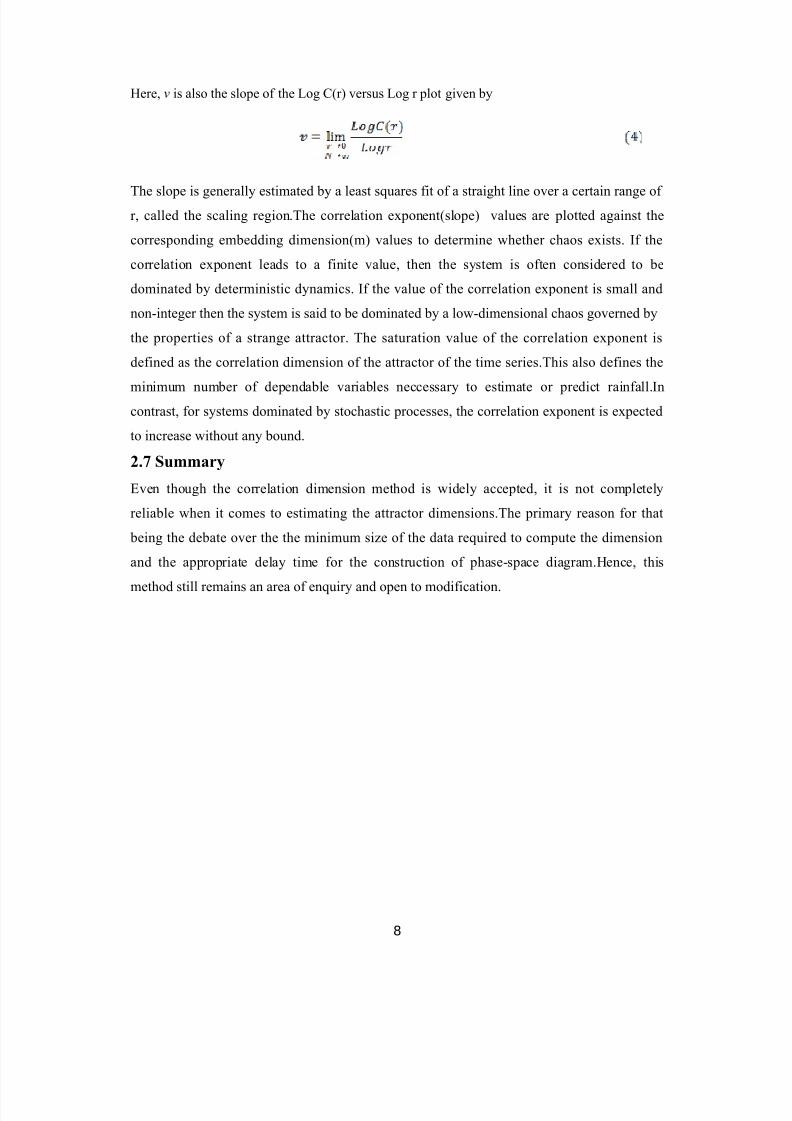
Figure 2 shows the variation of the rainfall series of different time scales at 3 different

stations of koyna dam.The correlation functions are computed for the 9 different time series

using the correlation dimension method.Using the values of correlation function(C(r)) and the

radius(r), the values of correlation expoenent is computed.The delay time , for the phase-

9

http://en.wikipedia.org/wiki/Dam

http://en.wikipedia.org/wiki/Maharashtra

http://en.wikipedia.org/wiki/India

http://en.wikipedia.org/wiki/Koyna_Nagar

http://en.wikipedia.org/wiki/Western_Ghats

http://en.wikipedia.org/wiki/Chiplun

http://en.wikipedia.org/wiki/Karad

http://en.wikipedia.org/wiki/Hydroelectric

http://en.wikipedia.org/wiki/Megawatt

http://en.wikipedia.org/wiki/Dam

http://en.wikipedia.org/wiki/Maharashtra

http://en.wikipedia.org/wiki/India

http://en.wikipedia.org/wiki/Koyna_Nagar

http://en.wikipedia.org/wiki/Western_Ghats

http://en.wikipedia.org/wiki/Chiplun

http://en.wikipedia.org/wiki/Karad

http://en.wikipedia.org/wiki/Hydroelectric

http://en.wikipedia.org/wiki/Megawatt



space reconstruction is computed using the auto-correlation function method and is taken as

the lag time at which the auto-correlation function first crosses the zero line.

10



Figure 2: Variation of rainfall series at Three Stations at Koyna Dam.

11



Figure 2: Variation of rainfall series at Three Station at Koyna Dam.

12



Figure 2: Variation of rainfall series at three Stations at Koyna Dam.

13




14




Figure 3 shows the Phase-space Diagram for different rainfall series.

15



Figure 3:Phase-Space diagrams for different rainfall series

A phase space diagram gives us the relationship between two subsequent data points.This is

done by offsetting a time series by a certain amount called as the delay time.The original time

series and the offset one is then taken and ploted on the X and Y axis respectively.

In the above figures, we see that there is a well defined attractor for each series, suggesting

the possibility of deterministic dynamics.

However, phase-space reconstruction is neccessary with an approriate delay time as only then

can we obtain the best separation of neighbouring trajectories within the minimum

embedding space.This optimum delay time calculated using the Auto-correlation Function.

The Autocorrelation function for different time series of the 3 stations is given below in

figure 4.

Station-1 Station-2 Station-3

16



Station 1 Station 2 Station 3

Figure 4 shows the variation of the auto-correlation function against the lag time for different

time series.

The autocorrelation function can be used for the following two purposes:

17



a) To detect non-randomness in data.

b) To identify an appropriate time series model if the data is not random.

Given measurements, Y 1, Y 2, ..., Y N at time X 1, X 2, ..., X N , the lag k autocorrelation function isdefined as

_ _

1

_ 2

1

( )( )

( )

N k

i i k

i

k N

i

i

Y Y Y Y

r

Y Y

−

+

=

=

− −

=

−

∑

∑(4)

Although the time variable, X , is not used in the formula for autocorrelation, the assumption

is that the observations are equi-spaced. Autocorrelation function will vary between -1 and

+1, with values near 1± indicating stronger correlation.

Autocorrelation is a correlation coefficient. However, instead of correlation between two

different variables, the correlation is between two values of the same variable at times X i and

X i+k .

When the autocorrelation is used to detect non-randomness, it is usually only the first (lag 1)

autocorrelation that is of interest. When the autocorrelation is used to identify an appropriate

time series model, the autocorrelations are usually plotted for many lags.

The optimum delay time for the phase-space reconstruction is taken as the lag time at which

the auto-correlation function first crosses the zero mark.The significance of the

autocorrelation function assuming zero value is that after that there is no correlation between

the different pair of points.

Let us take the example of the daily time series of station 1.

18



The autocorrelation function for the daily series fo station 1 is plotted in Fig 5 above. The

autocorrelation function approaches 1.0 when the lag time is zero signifying 100%

correlation. This is because at zero lag time the data is being compared with itself. As the lag

time increases the autocorrelation function decreases exponentially and finally assumes zero

value at 37 days. After this point there is no subsequent correlation between the data. Hence,

37 days is taken as the delay time for the phase-space reconstruction.

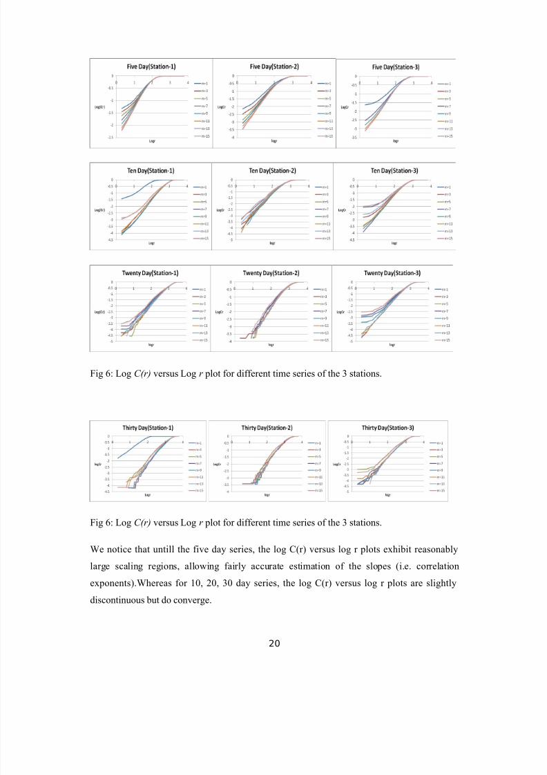
Figure 6 now shows the relationship between the correlation function, C(r), and the radius, r,

for the embedding dimensions, m, from 1 to 15, with a step of 2, for different time series of the 3 stations.The log C(r) versus log r plots indicate clear scaling regions that allow fairly

accurate estimates of the correlation exponent.

19





Figure 7 represents the relationship between the correlation exponent values and the

embedding dimension values for the 9 different rainfall series for the 3 stations.

Fig 7(a) Relationship between correlation exponent and embedding dimension.


21




We notice that for all the series, the correlation exponent value increases with the embedding

dimension up to a certain dimension, beyond which it gets saturated.This is an indication of

the existence of deterministic dynamics.The saturation values of the correlation exponent for

the three different stations are 2.1, 5.2 and 2.1 respectively.The finite correlation dimensions

obtained for the 9 series indicate that they all exhibit chaotic behaviour.This implies the

applicability of a chaotic approach for the transformation of rainfall data from one scale to

another.

3.3 Results

The (correlation) dimension of a time series represents the variability or irregularity of the

values in the series. A series with a high variability in values provides a higher dimension,

which, in turn, indicates higher complexity in the dynamics of the process. A low dimension

would be the result of low variability, indicating that the dynamics of the process are less

complex.The dimension results obtained above indicate that the rainfall series at all the above

scales exhibitlow variability.The correlation dimension values of below 2.1, 5.2 and 2.1

indicate that the number of dominant variables involved in the dynamics of the rainfall of the

corresponding stations are 3, 6 and 3 respectively.

22



The correlation dimension values for lower time scale series, saturate at a lower value as

compared to that for a higher time scale series.This proves that there is deterministic chaos in

the lower time scale series.

The above result of the value of correlation dimesnion in the dynamics of a rainfall series at

two of the above stations as 2.1, indicates that the correlation dimension method may have

some serious limitaions. The correlation dimension method is based on the assumption that

the time series is infinite and noise-free. Therefore, the application of this method to rainfall

series, which are always finite and contaminated by noise (e.g. measurement error), may

sometimes provide misleading results. For example, a finite and small data set may

underestimate the actual dimension (e.g. Havstad and Ehlers, 1989), whereas the presence of

noise may result in an overestimation of the dimension (e.g. Schreiber and Kantz, 1996).

Chapter 4

Conclusion

The belief that the estimation of the correlation dimension requires a large data set is based

on the assumption that the data size depends on the embedding dimension used in the

phase-space reconstruction. However, Sivakumar (2000) reveals that the data size depends on

the type and dimension of the underlying process, rather than the embedding dimension. The

sizes of the rainfall series considered in the present study and the dimension results obtained

may also be used to explain the above point. The higher resolution rainfall series, such as

daily, 2-day etc., are significantly larger in size than that of the lower resolution series, but

23



yield significantly lower dimensions than those of the lower resolution series. In other words,

the dimension estimate increases with a decreasing data size and vice versa. This suggests

that the data size could have only very little influence, if any at all, on the dimension estimate

and, therefore, the chances of underestimation of the dimension for the higher resolution

series (compared to the others) may be very limited.

The fact that the correlation dimension method yielded finite dimension values of 4.82, 5.26,

6.42, and 8.87 for the daily, 2-day, 4-day and 8-day rainfall series respectively suggests that

all of the above rainfall series exhibited chaotic behaviour. Hence, the transformation process

between these scales might also be chaotic; however, such an interpretation must be further

substantiated. Investigation of any parameter that connects the above rainfall series could be

useful. The distribution of rainfall from one scale to another is one such important parameter,

studies of which might lead to additional information regarding the behaviour of

transformation processes at Koyna Dam.

Although the present study did not answer concusively the existence of chaotic behaviour in

the dynamics of rainfall transformation process between different scales, it has provided

some clues so as not to exclude such a possibility and justifies continuation of the

investigation to confirm the existence of a chaotic component in the transformation

process. If confirmed, the presence of chaotic behaviour could provide interesting openings

for a better understanding of the rainfall transformation process.

References

Berndtsson, R., Jinno, K., Kawamura, A., Olsson, J. and Xu, S., 1994. Dynamical systems

theory applied to long-term temperature and precipitation time series. Trends Hydrol., 1,

291–297.

Grassberger, P. and Procaccia, I., 1983. Measuring the strangeness of strange attractors.

Physica D, 9, 189–208.

Havstad, J.W. and Ehlers, C.L., 1989. Attractor dimension of nonstationary dynamical

systems from small data sets. Phys. Rev. A, 39, 845–853.

Holzfuss, J. and Mayer-Kress, G., 1986. An approach to errorestimation in the application of dimension algorithms. In: Dimensions and Entropies in Chaotic Systems, G. Mayer-Kress,

24



(Ed.). Springer, New York, USA, 114–122.

Jayawardena, A.W. and Lai, F., 1994. Analysis and prediction of chaos in rainfall and stream

flow time series. J. Hydrol., 153, 23–52.

Koutsoyiannis, D. and Pachakis, D., 1996. Deterministic chaos versus stochasticity inanalysis and modeling of point rainfall series. J. Geophys. Res., 101, 26441–26451.

Krasovskaia, I., Gottschalk, L. and Kundzewicz, Z.W., 1999. Dimensionality of Scandinavian

river flow regimes. Hydrolog. Sci. J., 44, 705–723.

Porporato, A. and Ridolfi, L., 1997. Nonlinear analysis of river flow time sequences. Water

Resour. Res., 33, 1353–1367.

Puente, C.E. and Obregon, N., 1996. A deterministic geometric representation of temporal

rainfall: Results for a storm in Boston. Water Resour. Res., 32, 2825–2839.

Rodriguez-Iturbe, I., De Power, F.B., Sharifi, M.B. and Georgakakos, K.P., 1989. Chaos in

rainfall. Water Resour. Res., 25, 1667–1675.

Schreiber, T. and Kantz, H., 1996. Observing and predicting chaotic signals: Is 2% noise too

much? In: Predictability of Complex Dynamical Systems, Yu.A. Kravtsov, and J.B. Kadtke,

(Eds.). Springer Series in Synergetics, Springer, Berlin, Germany, 43–65.

Sivakumar, B., 2000. Chaos theory in hydrology: important issues and interpretations. J.

Hydrol., 227, 1–20.

Sivakumar, B., Liong, S.Y., Liaw, C.Y. and Phoon, K.K., 1999a. Singapore rainfall behavior:

Chaotic? J. Hydrol. Eng., ASCE , 4, 38–48.

Sivakumar, B., Phoon, K.K., Liong, S.Y. and Liaw, C.Y., 1999b. A systematic approach to

noise reduction in hydrological chaotic time series. J. Hydrol., 219, 103–135.

Stehlik, J., 1999. Deterministic chaos in runoff series. J. Hydrol. Hydromech., 47, 271–287.

Takens, F., 1981. Detecting strange attractors in turbulence. In: Dynamical Systems and

Turbulence, D.A. Rand, and L.S. Young, (Eds.). Lecture Notes in Mathematics, 898,

Springer, Berlin, Germany, 366–381.

Tsonis, A.A., Elsner, J.B. and Georgakakos, K.P., 1993. Estimating the dimension of weather

and climate attractors: important issues about the procedure and interpretation. J. Atmos. Sci.,

50, 2549– 2555.

Tsonis, A.A., Triantafyllou, G.N., Elsner, J.B., Holdzkom II, J.J. and Kirwan Jr., A.D., 1994.

An investigation of the ability of nonlinear methods to infer dynamics from observables.

Bull.

Amer. Meteorol. Soc., 75, 1623–1633.

Mayank Mehta, BTP Report IITB.

Documents

Dimensions required to estimate the rainfall in a region