Embed Size (px)
Citation preview
TRANSPORTATION RESEARCH RECORD 1224 67
Dimensionless Hydrograph Method of Simulating Flood Hydrographs
v. B. SAUER
The dimensionless hydrograph method is a simple, easy-to-use technique for simulating an average, or typical, hydrograph that corresponds to a given peak discharge. The method has been successfully tested and applied to both rural and urban streams in the states of Georgia, Tennessee, Alabama, South Carolina, Ohio, Missouri, and Arkansas. Most studies found that the dimensionless hydrograph developed for the Georgia study, which is nearly identical to a theoretical dimensionless hydrograph developed nationwide for urban streams, will apply to streams in the other study areas. Only in the Coastal Plain area of South Carolina and the lowlands of west Tennessee were dimensionless hydrographs found to be significantly different. An important parameter for the use of the dimensionless hydrograph method is the basin lagtime. Each of the studies developed regression equations that relate lagtime to basin characteristics. The other parameter needed to apply the method is peak discharge. The accuracy of the dimensionless hydrograph method varies from state to state, but in general the width at 50 and 75 percent of the peak discharge had standard errors in the range of 20 to 40 percent. For large floods at ungauged sites, the standard errors were between about 30 and 60 percent and represented the combined errors using lagtime regressions, peak discharge regressions, and the dimensionless hydrograph. The report also contains hydrograph width relations that can be used to determine the elapsed time that a specified discharge would be exceeded. Some investigators included regression equations for estimating flood volumes; however, flood volumes also can be computed by integrating the area beneath the simulated hydrograph, or by applying an equation that yields virtually the same result as the integration method.
The design of transportation structures, flood detention structures, and other flood control structures requires an estimate of flood peak discharges, flood hydrographs, and flood volumes for specified design probabilities. The U.S. Geological Survey (Geological Survey) has cooperated with state highway departments, the FHWA, and other state and federal agencies to provide flood data and flood frequency analyses to meet the needs of design engineers. Much of the past work has been for the purpose of providing flood peak information. Recently, however, the Geological Survey has been working on projects to develop methods of estimating flood hydrographs and flood volumes. Projects have been completed for Georgia, Alabama, Ohio (urban), and central Tennessee. Projects are nearing completion in South Carolina, Ohio (rural), Missouri, Arkansas, and east and west Tennessee. A nationwide urban hydrograph project has also been completed. Each of these studies uses a similar approach that provides a simple, easy-to-use dimensionless hydrograph that can be converted to a design hydrograph for any design peak discharge. In some
U.S. Geological Survey, Richard B. Russell Federal Building, 75 Spring Street, S.W., Suite 772, Atlanta, Ga. 30303.
of these studies, methods are also provided for estimating flood volumes.
The purpose of this paper is to describe the dimensionless hydrograph method and to compare the results obtained in the states in which projects have been completed or are under way. Results from the states of Georgia, Alabama, Tennessee, South Carolina, Ohio, Missouri, and Arkansas will be compared. The nationwide urban hydrograph results will also be compared with the individual state results. Comparisons will be made of the dimensionless hydrograph, hydrograph width relations, lagtime equations, and volume equations.
The results from uncompleted studies in South Carolina, Ohio (rural), Missouri, Arkansas, and east and west Tennessee are preliminary and subject to revision.
DESCRIPTION OF METHOD
The dimensionless hydrograph method is specifically designed to be easy to use and to produce a typical hydrograph that represents average runoff for a specified peak discharge. The hydrograph peak discharge will be exactly the same as the peak discharge for the design recurrence interval, i.e., a 50-year or 100-year discharge. There are three essential parts to the dimensionless hydrograph method: (a) the peak discharge for which a hydrograph is desired, (b) the basin lagtime, and ( c) the dimensionless hydrograph itself.
The peak discharge can be an actual observed peak if it is desired to fit an average hydrograph to some known peak. In this case, the analyst should be aware that the fitted hydrograph will not necessarily reproduce the actual hydrograph, nor is it intended to. The resultant hydrograph will simply be an average hydrograph that represents average conditions. On the other hand, most design applications will use a peak discharge representative of some specified recurrence interval. Peak discharges of this type can be determined independently. The Geological Survey has defined regression equations for this purpose throughout the United States. These equations are based on actual streamflow records and log Pearson type III frequency distributions. They are available through published reports and soon will be available through computer programs. Other methods of defining the peak discharge to be used in the dimensionless hydrograph method are acceptable and are the choice of the analyst.
Basin lagtime is defined as the elapsed time, in hours,Jrom the center of mass of rainfall excess to the center of mass of the resultant runoff hydrograph. This is the most difficult estimate to make for the dimensionless hydrograph method

68
Q_
00.80 "---.. a
.SJ 0.60 +-' 0
G'.'.:
~0.40 L
0 ...c
(_)
.~ 0.20 0
Georgia
\ Q.QQ ~~~1.J.J.J.,,Jl!ll!llt11111111!1 11 i 11~ IJ..J-LJ
0.00 0.50 1 .00 1.50 2.00 2.50
Time Ratio, t/LT FIGURE 1 Dimensionless hydrograph for Georgia.
because lagtime is highly variable, depending on numerous basin conditions such as basin size, basin and channel slope , soil conditions, cover, basin storage (reservoir, swamps, and detention ponds), urbanization, channel conditions, channel modifications, and other factors. Generally lagtime is considered to be constant for a given basin, and not variable with the size of the runoff event. Most of the Geological Survey hydrograph projects have followed this concept and use a constant lagtime for all floods for a given basin. It has been observed, however, that in some basins lagtime will vary with the size of the runoff event. In these cases, lagtime will decrease as the size of the runoff event increases. The uncertainty in estimating lagtime, even for gauged basins, is large, and consequently most of the error in the estimated hydrographs results from the errors in lagtime. Regression equations have been developed for the areas of each of the Geological Survey studies, including some urban areas, and these equations can be used to estimate lagtime for ungauged basins.
The third, and final component needed to use the dimensionless hydrograph method, is the dimensionless hydrograph ordinates. Figure 1 is a plot of the dimensionless hydrograph defined for use in the state of Georgia by Inman (1). Note that the ordinate scale is a dimensionless ratio of discharge (Q) to peak discharge (Qp), and the abscissa scale is a dimensionless ratio of time (t) to lagtime (LT). This dimensionless hydrograph was developed by analyzing several hundred actual flood hydrographs and reducing them to unit hydrographs and finally to the dimensionless hydrograph as described by Inman (1). A paper describing the procedure was presented in 1986 to the Transportation Research Board and has been published (2).
A feature, and advantage, of the dimensionless hydrograph method is that it does not require any kind of rainfall or rainfall excess analysis. The derivation of the dimensionless hydrograph was based on a generalization of rainfall duration by considering duration as a fraction of lagtime. By comparing synthesized hydrograph widths based on different values of duration with observed hydrograph widths, it was found that the optimum value of duration (minimum standard error) was equal to one-half the value of lagtime for most of the study
TRANSPORTATION RESEARCH RECORD 1224
areas . Consequently, the dimensionless hydrograph method contains an indirect consideration of rainfall duration that will produce an average hydrograph for the selected peak discharge. On the other hand, it cannot be expected to reproduce actual flood hydrographs because the actual rainfall is not considered in the computations. Removing rainfall and rainfall excess computations from the dimensionless hydrograph method makes the method simple and easy to apply.
Application of the dimensionless hydrograph to derive an average, or typical, hydrograph for a specified peak discharge, Qp , is a simple case of multiplication. The hydrograph discharge ordinates, in cubic feet per second, are computed by multiplying each of the discharge ratios, Q!Qp, times the peak discharge, Qp. Likewise, the time, in hours, for each discharge is computed by multiplying the time ratios, t!LT, times the basin lagtime, LT. The resultant hydrograph will have a peak discharge equal to the specified, or design, peak discharge and can be assumed to be typical for that recurrence interval.
COMPARISON OF DIMENSIONLESS HYDROGRAPHS
The first Geological Survey statewide dimensionless hydrograph study was made by Inman (1) using streamflow data from 355 flood events recorded at 80 gauging stations in Georgia. These data included sites located in all parts of the state, including mountains, coastal plains, and urban areas. Inman (1) found that the optimum value of rainfall duration was onehalf of lagtime. Testing and verification of the dimensionless hydrograph involved the use of 138 additional storm events at 37 different gauging stations. Because it involved the use of an extensive data base for the development and testing of the dimensionless hydrograph, this study is considered the primary basis of comparison for other studies. In fact, several of the other studies have adopted the Georgia dimensionless hydrograph for use in their states.
A nationwide urban hydro graph study was made by Stricker and Sauer (3) using a theoretical approach. In that study , unit hydrographs were computed for 62 urban gauging stations located in Georgia, Pennsylvania, Tennessee, Colorado, Missouri, Oklahoma, Oregon , and Texas. The method of Clark (4) was used to derive a theoretical unit hydrograph for each station. These unit hydrographs were transformed to a generalized rainfall excess duration of one-third lagtime and then reduced to dimensionless terms. The duration of one-third lagtime was an arbitrary choice. However, a comparison of the final dimensionless hydrograph to the Georgia dimensionless hydrograph (Figure 2) shows that the two hydrographs are similar and, in fact, are almost identical. The nationwide urban hydrograph is slightly more narrow, and this is probably because it is based on a duration of one-third lagtime as opposed to the one-half lagtime of the Georgia hydrograph. The application of either of these hydrographs will produce similar results, and for practical purposes they are considered equal.
The Tennessee hydrograph project was divided into two parts, one for central Tennessee and the other for east and west Tennessee. In the central Tennessee study, Robbins (5) used a small, distributed data base and the analytical techniques developed in Georgia to derive an average dimen-

Sauer
-- Georgia - - Nationwide Urban
o_ 00.80
"'-0
-.2 0.60 -+-' 0
O'.'.
~0.40 L 0
..i:::: u .~ 0.20 0
1 I
I \
\
\ \ .
\
0.00 ~ ......... ~ ................. '-'-'-_._,_._._._._._. .......................................................... ._._. ......... -'-'-' 0 .00 0.50 1.00 1.50 2.00 2.50
Time Ratio, t/LT FIGURE 2 Comparison of Georgia and nationwide urban dimensionless hydrographs.
o_ 00.80
"'-0
.S'. 0.60 -+-' 0
O'.'.
~0.40 L
0 ..i:::: u .~ 0 .20 0
\ \
\ \
\ \
0.00 ............... ......_....._.__._._..,_._,_._._...._,_,__._~1 I I I I I I I I I I I I !J.....Li.....l
0.00 0.50 1.00 1.50 2.00
Time Ratio, t/LT FIGURE 3 Comparison of Georgia and west Tennessee dimensionless hydrographs.
2.50
sionless hydrograph. He compared and tested this dimensionless hydrograph with the Georgia dimensionless hydrograph and found that it was essentially the same. Consequently, he adopted the Georgia dimensionless hydrograph for use in central Tennessee. In the second Tennessee study (Gamble, unpublished data), it was also found that the Georgia dimensionless hydrograph was applicable to east Tennessee streams. They used a selected data base to compute an average dimensionless hydrograph that was found to be nearly identical to the Georgia hydrograph. The situation was different, however, in west Tennessee where the dimensionless hydrograph was found to be considerably wider than the Georgia hydrograph. Figure 3 is a comparison of the west Tennessee dimensionless hydrograph, developed from 38 flood events at 10
69
gauging stations, with the Georgia dimensionless hydrograph. The reason for the departure from the basic dimensionless hydrograph developed in Georgia may be related to the topography of west Tennessee, where relief is much less than in east and central Tennessee and most of Georgia. In addition, considerable channel modifications that affect runoff distribution have been performed on the west Tennessee streams.
In the Alabama study, Olin and Atkins (6) developed dimensionless hydrographs by using the Georgia method with data from 76 flood events at 27 rural gauging stations. They also made similar computations for 44 flood events at 10 urban stations. These stations were selected because they were representative of all hydrologic areas in Alabama. Both the rural and urban dimensionless hydrographs compared closely with the Georgia dimensionless hydrograph, and that hydrograph was adopted for use in Alabama.
In South Carolina, 188 flood events recorded at 49 rural gauging stations throughout South Carolina were used to develop regionalized dimensionless hydrographs. Bohman (unpublished data) found a significant difference in the dimensionless hydro graphs for each of three regions-the Blue Ridge province, the Piedmont province, and the Coastal Plain province south of the fall line. Only in the Piedmont province did he find that the dimensionless hydrograph was nearly the same as that for the Georgia dimensionless hydrograph, and even so, he opted to use the hydrograph derived from the South Carolina data. See Figure 4 for a comparison of this Piedmont dimensionless hydrograph to the Georgia hydrograph. In the Blue Ridge he found that the dimensionless hydrograph was more narrow than the Georgia hydrograph, and that the optimum duration was one-third lagtime rather than one-half lagtime. The shorter duration may account, at least partially, for the more narrow width of the Blue Ridge hydrograph. See Figure 5 for a comparison of the Blue Ridge hydrograph to the Georgia hydrograph. In the Coastal Plain south of the fall line, the dimensionless hydrograph was found to be considerably wider than the Georgia hydrograph (see Figure 6) .
o_ 00.80
"'-0
.2 0.60 -+-' 0
O'.'.
~0.40 L
0 ..i:::: u (f) 0.20
0
0. 00 ~ ......... -~._._. ................................... ~ ............................................................. ~~ ......... 0.00 0.50 1.00 1.50 2.00
Time Ratio, t/LT FIGURE 4 Comparison of Georgia and South Carolina Piedmont dimensionless hydrographs.
2.50

70
0.. 00.80
"' o
.Q 0.60 -+-' n
er::
~0.40 L
0 ..r::: u
.'.!:! 0.20 0
\
I
-- Georgia - - South Carolina-
Blue Ridge
0 .00 .............................................. ~ ......... ~ ................... ~ ................... ~ ....................................... ~ 0.00 0.50 1.00 1.50 2.00 2.50
Time Ratio, t/LT FIGURE 5 Comparison of Georgia and South Carolina Blue Ridge dimensionless hydrographs.
0.. 00.80 r
"' o
.Q 0.60 -+-' 0
er::
~0.40 L
0 ..r::: u (/) 0.20
0
I
I I
\ - - Georgia \ - - South Carolina-
\ South of Fall Line
\ \
\ \
\ \
\ \
\
' \
0. 00 ~ .......... ~~. ~ .......... ~ .......... ~~ .......... ~u.J.. ................... ~ ............................. ~ 0.00 0.50 1.00 1.50 2.00 2.50
Time Ratio, t/LT FIGURE 6 Comparison of Georgia and South Carolina, south of the fall line, dimensionless hydrographs.
Like the west Tennessee study, this may reflect the flat slopes and small topographic relief. In addition, there is considerable surface storage in the Coastal Plains area, as well as many channel modifications. All of these factors may combine in some way to result in comparatively wide hydrograph shapes. Although it was decided to use three separate dimensionless hydrographs for South Carolina, the use of the Georgia hydrograph could be used with acceptable standard errors. There would, however, be a bias in the Blue Ridge province and the Coastal Plains province if the Georgia hydrograph were used.
Investigators in Arkansas took a somewhat different approach to develop an average dimensionless hydrograph for 18 gauging stations throughout the state (Neely, unpublished data).
TRANSPORTATION RESEARCH RECORD 1224
0.. 00.80
"' o
.Q 0.60 -+-' (J
er::
~0.40 L
0 ..r::: u
.'.!:! 0.20 0
I
/
\ \
,, \ \
I I I I I I I
\
' . \ \
\ \
\
Georgia - - - Missouri
\ \
' '
0. 00 .............................................. ~ ................... ~ ................... ~ .......... ~~·
0.00 0.50
Time 1.00 1.50 2.00
Ratio. t/LT FIGURE 7 Comparison of Georgia and Missouri dimensionless hydrographs.
2.50
They reduced actual flood hydrographs to dimensionless terms rather than first defining unit hydro graphs as done in the other state studies. Even so, they found that the average dimensionless hydrograph as defined for the 18 stations was essentially the same as the Georgia hydrograph, so they decided to use the Georgia hydrograph for Arkansas because it is defined from considerably more data. The Arkansas data were obtained only from rural gauging stations.
An urban hydrograph study in Ohio by Sherwood (7) has been completed, and another Ohio study for small rural basins is in progress (Sherwood, unpublished data). In the urban study, he found that the dimensionless hydrograph developed by Stricker and Sauer (3) for the nationwide urban flood study was applicable to Ohio urban sites. This hydrograph is similar to the Georgia hydrograph as seen in Figure 2. In the study for small rural basins, he used 96 flood events from 32 gauging stations to verify that the Georgia dimensionless hydrograph is applicable in Ohio.
Preliminary results from the hydrograph project under way in Missouri (Becker, unpublished data) indicate that the dimensionless hydrograph developed from data in Missouri compares closely with the Georgia dimensionless hydrograph; however, the dimensionless hydrograph developed from the Missouri data will be used. Figure 7 shows a comparison of the Missouri hydrograph to the Georgia hydrograph.
Table 1 shows the ordinates for the various dimensionless hydrographs. The ordinates have been purposely aligned so that the maximum ratio of Q/Qp coincides for each hydrograph.
COMPARISON OF EQUATIONS FOR ESTIMATING BASIN LAGTIME
An important factor in the dimensionless hydrograph method is basin lagtime. As already mentioned, this is a difficult factor to estimate for a drainage basin. For gauged basins, lagtime can be estimated from observed records of rainfall and runoff.
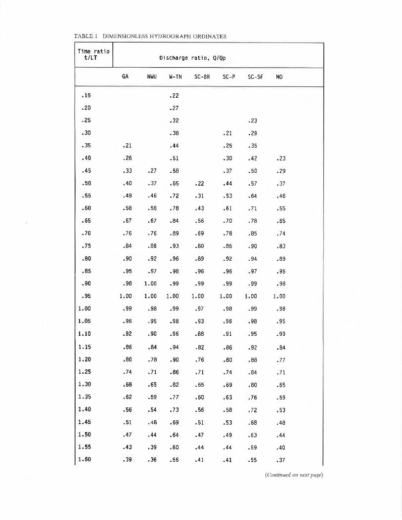
TABLE 1 DIMENSIONLESS HYDROGRAPH ORDINATES
Time ratio t/LT Discharge ratio, Q/Qp
GA NWU W-TN SC-BR SC-P SC-SF MO
.15 .22
.20 .27
.25 .32 .23
.30 .38 .21 .29
.35 .21 .44 .25 .35
.40 .26 .51 .30 .42 .23
.45 .33 .27 .58 .37 .50 .29
.50 .40 .37 .65 .22 .44 .57 .37
.55 .49 .46 .72 .31 .53 .64 .46
.60 .58 .56 .78 .43 .61 .71 .55
.65 .67 .67 .84 .56 .70 .78 .65
.70 .76 .76 .89 .69 .78 .85 .74
.75 .84 .86 .93 .80 .86 .90 .83
.80 .90 .92 .96 .89 .92 .94 .89
.85 .95 .97 .98 .96 .96 .97 .95
.90 .98 1.00 .99 .99 .99 .99 .98
.95 1.00 1.00 1.00 1.00 1.00 1.00 1.00
1.00 .99 .98 .99 .97 .98 .99 .98
1.05 .96 .95 .98 .93 .96 .98 .95
1.10 .92 .90 .96 .88 .91 .95 .90
1.15 .86 .84 .94 .82 .86 .92 .84
1.20 .80 .78 .90 .76 .80 .88 .77
1.25 .74 .71 .86 .71 .74 .84 .71
1.30 .68 .65 .82 .65 .69 .80 .65
1.35 .62 .59 .77 .60 .63 .76 .59
1.40 .56 .54 .73 .56 .58 .72 .53
1.45 .51 .48 .69 .51 .53 .68 .48
1.50 .47 .44 .64 .47 .49 .63 .44
1.55 .43 .39 .60 .44 .44 .59 .40
1.60 .39 .36 .56 .41 .41 .55 .37
(Continued on next page)

72 TRANSPORTATION RESEARCH RECORD 1224
TABLE 1 (continued)
Time ratio t/LT Discharge ratio, Q/Qp
GA NWU W-TN SC-BR SC-P SC-SF MO
1.65 .36 .32 .53 .38 .37 .51 .34
1.70 .33 .30 .49 .35 .34 .48 .31
1.75 .30 .46 .33 .32 .44 .28
1.80 .28 .42 .30 .29 .40 .26
1.85 .26 .39 .28 .27 .37 .24
1.90 .24 .36 .26 .25 .34 .22
1.95 .22 .33 .24 .23 .31 .20
2.00 .20 .30 .23 .21 .28
2.05 .28 .21 .25
2.10 .25 .20 .23
2.15 .23 .20
2.20 .21
[GA=Georgia, NWU=Nationwide urban, W-TN=West Tennessee, SC-BR=South Carolina Blue Ridge, SC-P=South Carolina Piedmont, SC-SF=South
Carolina south of fall line, and MO=Missouri]
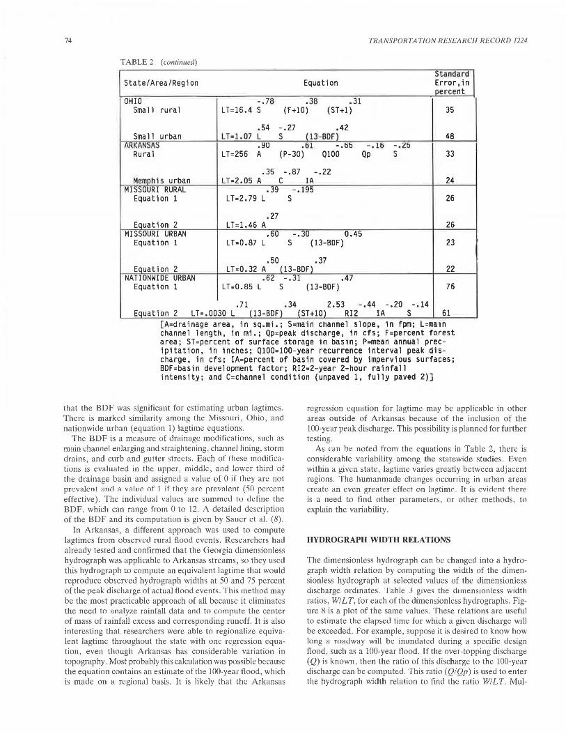
Even so, there is a great deal of uncertainty because one must compute the time of the center of mass of rainfall excess and the corresponding time of the center of mass of direct runoff, which vary from storm to storm. Numerous factors enter into these computations, such as the magnitude and distribution of rainfall excess, infiltration, and extraction of base flow from the totai runoff hydrograph. The subjective nature of these factors makes interpretation difficult and can lead to errors in the computed lagtime. For ungauged basins, the problem is even more difficult. Generally, lagtime for ungauged basins is estimated from equations or graphs that relate lagtime to basin parameters such as drainage area size, length, slope, vegetal cover, storage in reservoirs and swamps, and, in some cases, even size of runoff event. Standard errors are, however, generally large. In addition, there seem to be regional differences that cannot be accounted for with the usual array of measurable basin parameters. Consequently, it becomes necessary to segment the estimating equations and graphs by region. Table 2 is a listing and comparison of the various equations developed by regression analysis for the hydrograph studies.
In all of the equations except Ohio (rural) there is a measure of basin size, either drainage area or main channel length. For rural basins in Ohio the size of the basins was limited to a maximum of 6.5 mi2
; consequently, size did not prove significant in the regression with lagtime. It was found that main channel slope, percent of forest area in the basin, and percent
of storage in the basin were the significant factors for estimating lagtime in rural areas up to 6.5 mi2 in Ohio. Main channel slope also proved significant in a number of the other equations, both rural and urban. In the Arkansas and South Carolina studies, it was found that the peak discharge of a flood hydrograph is related to the lagtime of that hydrograph. in each of these studies, the equations show that for a given drainage basin, the flood hydrographs with large peaks have shorter lagtimes than flood hydrographs with small peaks. This difference can be logically explained because, in many drainage systems, the main channel tends to meander within a flood plain that is comparatively straight. Consequently, as the size of the flood increases, the flow path shortens and velocities increase, which result in shorter travel times and thus shorter lagtimes. In the South Carolina study, equations were developed for average basin lagtime and for discharge adjusted lagtime. Both sets of equations are shown in Table 2, but standard errors were computed only for the average lagtime equations.
For urban basins, the parameters for estimating lagtime are essentially the same as those for rural basins, except that the equations contain some measure of urbanization. Most of the equations use the percent of basin covered by impervious surfaces for the urbanization index. The nationwide urban equation developed by Sauer et al. (8) also contains the basin development factor (BDF) as well as several other parameters. In the urban studies in Ohio and Missouri, it was found
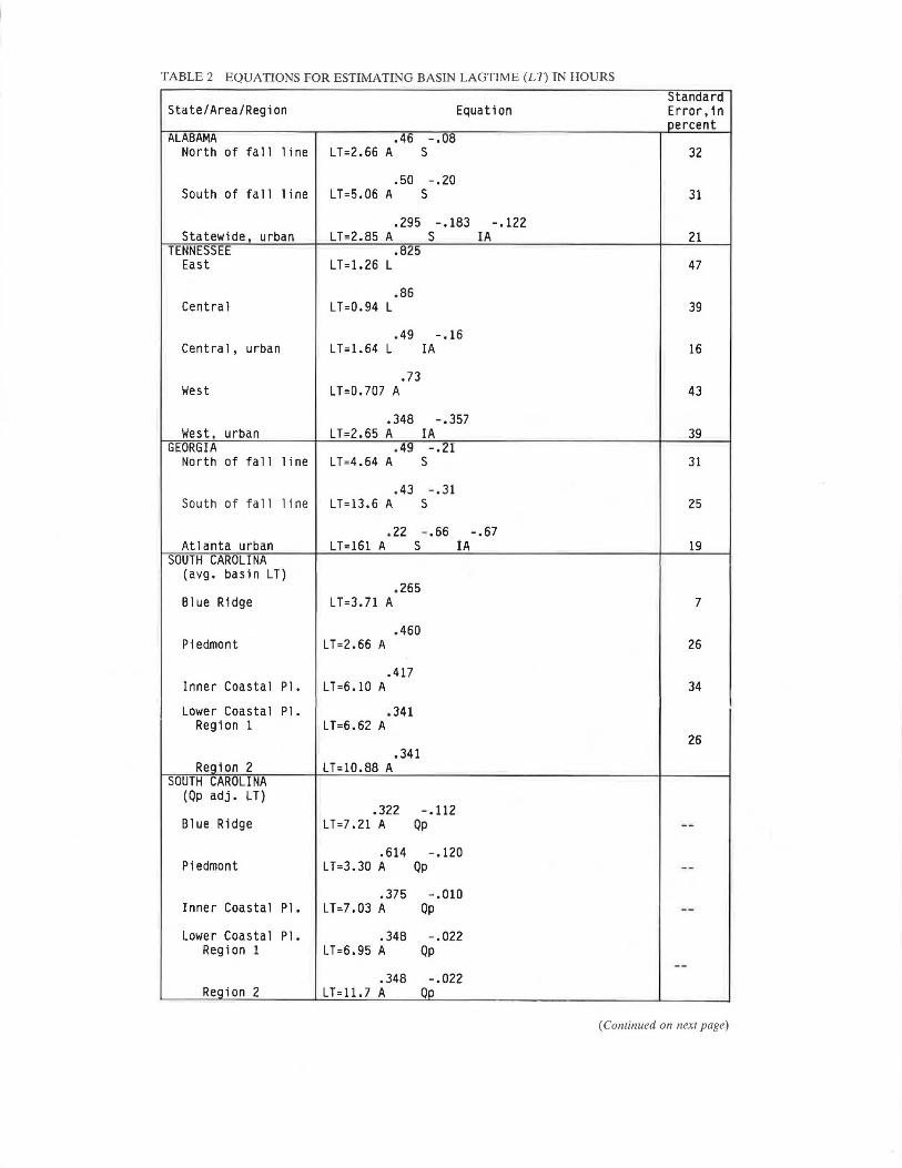
TABLE 2 EQUATIONS FOR ESTIMATING BASIN LAGTIME (LI) IN HOURS
Standard State/Area/Region Equation Error,in
percent ALABAMA .46 -.OB
North of fall line LT=2.66 A s 32
.50 -.20 South of fa 11 line LT=5.06 A s 31
.295 -.183 -.122 Statewide , urban LT=2.85 A s IA 21
TENNESSEE .82S East LT=l.26 L 47
.86 Central LT=0.94 L 39
.49 -.16 Central, urban LT=l.64 L IA 16
.73 West LT=0.707 A 43
.348 -.357 West , urban LT=2.65 A IA 39
GEORGIA .49 -.21 North of fall line LT=4.64 A s 31
. 43 -.31 South of fall line LT=l3.6 A s 25
.22 - .66 -.67 Atlanta urban LT=161 A s IA 19
SOUTH CAROLI NA (avg. basin LT)
.265 Blue Ridge LT=3.71 A 7
.460 Piedmont LT=2.66 A 26
.417 Inner Coastal Pl. LT=6.10 A 34
Lower Coastal Pl. .341 Region 1 LT=6.62 A
26 .341
Region 2 LT=l0.88 A SOUTH CAROLI NA
(Qp adj. LT) .322 -.112
Blue Ridge LT=7 .21 A Qp --.614 -.120
Piedmont LT=3.30 A Qp --.375 -.010
Inner Coastal Pl. LT=7.03 A Qp --Lower Coastal Pl. .348 -.022
Region 1 LT=6.95 A Qp --
.348 -.022 Region 2 LT=ll.7 A Qp
(Continued on next page)
74 TRANSPORTATION RESEARCH RECORD 1224
TABLE 2 (continued)
standard State/Area/Region Equation Error,in
oercent OHIO -.78 .38 .31
Small rural LT=16.4 S (F+lO) (ST+l) 35
.54 -.27 .42 Small urban LT=l.07 L s (13-BOF) 48
ARKANSAS .90 .61 -.ti!:> - .lb -.Z!> Rural LT=256 A (P-30) 0100 Op s 33
.35 -.87 -.22 Memphis urban LT=2.05 A c IA 24
MISSOURI RURAL .39 -.195 Equation 1 LT=2.79 L s 26
.27 Eauation 2 LT=l.46 A 26
MISSOURI URBAN .60 -.30 0.45 Equation 1 LT=0.87 L s (13-BDF) 23
.50 .37 Equation 2 LT=0.32 A (13-BDF) 22
NATIONWIDE URBAN .62 -.31 .47 Equation 1 LT=0.85 L s (13-BOF) 76
.71 .34 2.53 -.44 -.20 -.14 Equation 2 LT=.0030 L (13-BDF) (ST+lO) RI2 IA s 61
[A=drainage area, in sq.mi.; S=main channel slope, in fpm; L=ma1n channel length, in mi.; Op=peak discharge, in cfs; F=percent forest area; ST=percent of surface storage in basin; P=mean annual precipitation, in inches; 0100=100-year recurrence interval peak discharge, in cfs; IA=percent of basin covered by 1mperv1ous surfaces; BDF=basin development factor; RI2=2-year 2-hour rainfall intensity; and C=channel condition (unpaved 1, fully paved 2)]
that the BDF was significant for estimating urban lagtimes. There is marked similarity among the Missouri, Ohio , and nationwide urban (equation 1) lagtime equations.
The BDF is a measure of drainage modifications, such as main channel enlarging and straightening, channel lining, storm drains, and curb and gutter streets. Each of these modifications is evaluated in the upper, middle, and lower third of the drainage basin and assigned a value of 0 if they are not prevalent and a value of 1 if they ;ire prev;ilent (.SO percent effective). The individual values are summed to define the BDF, which can range from 0 to 12. A detailed description of the BDF and its computation is given by Sauer et al. (8).
In Arkansas, a different approach was used to compute lagtimes from observed rural flood events. Researchers had already tested and confirmed that the Georgia dimensionless hydrograph was applicable to Arkansas streams, so they used this hydrograph to compute an equivalent lagtime that would reproduce observed hydrograph widths at 50 and 75 percent of the peak discharge of actual tlood events. This method may be the most practicable approach of all because it eliminates the need to analyze rainfall data and to compute the center of mass of rainfall excess and corresponding runoff. It is also interesting that researchers were able to regionalize equivalent lagtime throughout the state with one regression equation, even though Arkansas has considerable variation in topography. Most probably this calculation was possible because the equation contains an estimate of the 100-year flood, which is made on a regional basis. It is likely that the Arkansas
regression equation for lagtime may be applicable in other areas outside of Arkansas because of the inclusion of the 100-year peak discharge. This possibility is planned for further testing.
As can be noted from the equations in Table 2, there is considerable variability among the statewide studies. Even within a given state, lagtime varies greatly between adjacent regions. The humanmade changes occurring in urban areas create an even greater effect on lagtime. It is evirlent there is a need to find other parameters, or other methods, to explain the variability .
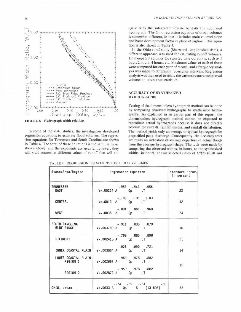
HYDROGRAPH WIDTH RELATIONS
The dimensionless hydrograph can be changed into a hydrograph width relation by computing the width of the dimensionless hydrograph at selected values of the dimensionless discharge ordmates. Table J gives the dimensionless width ratios, WI LT, for each of the dimensionless hydrographs. Figure 8 is a plot of the same values. These relations are useful to estimate the elapsed time for which a given discharge will be exceeded. For example, suppose it is desired to know how long a roadway will be inundated during a specific design flood, such as a 100-year flood. If the over-topping discharge (Q) is known, then the ratio of this discharge to the 100-year discharge can be computed. This ratio (Q/Qp) is used to enter the hydro graph width relation to find the ratio WILT. Mui-

Sauer
TABLE 3 HYDROGRAPH WIDTH RELATIONS
Discharge Ratio, Width ratios, WILT
Q/Qp
GA NWU W-TN SC-BR SC-P SC-SF MO
1.00 0.00 0.00 0.00 o.oo 0.00 0.00 o.oo .95 .22 .22 .34 .18 .22 .30 .19
.90 .32 .32 .49 .27 .32 .43 .29
.85 .40 . 40 .60 .34 .41 .55 .37
.80 .48 .46 .70 .42 .50 .65 .44
.75 .55 .53 .80 .48 .57 .74 .51
.70 .62 .59 .90 .54 .64 .83 .58
.65 .68 .66 .99 .61 .71 .92 .65
.60 .76 .72 1.09 .68 .79 1.02 .71
.55 . 83 .80 1.19 .74 .87 1.11 .79
.50 .91 .86 1.29 .84 .95 1.22 .86
.45 1.00 .95 1.40 .92 1.04 1.32 .94
.40 1.09 1. 01 1.52 1.02 1.14 1.43 1.03
.35 1.20 1.12 1.64 1.12 1.24 1.53 1.14
.30 1.33 1.23 1. 78 1.26 1. 38 1.65 1.26
.25 1.4 -- 1.93 1.41 1.55 1. 79 1.41
[GA=Georgia, NWU=Nationwide urban , W-TN=West Tennessee , SC-BR=South Carolina Blue Ridge, SC-P=South Carolina Piedmont, SC-SF=South
Carolina south of fall line, and MO=Missouri]
tiplying the WILT ratio times the estimated lagtime (LT) for the basin will yield an estimate of the inundation time, in hours.
where
V = flood volume (in.),
FLOOD VOLUMES
Qp = peak discharge (ft3/sec), LT = basin lagtime (hr),
A = drainage area, (mi2), and a = conversion constant.
75
Flood volumes corresponding to the hydrographs computed by the dimensionless hydrograph method can be computed by extending the ri ·ing and falling limb of the hydrograph to zero flow , and then integrat ing the area beneath the hydrographs. Volume. computed in thi manner, like the hydrograph itself, are ' imply an averag , or typical, volume for the design peak discharge. It can be assumed that the recurrence intervals of such volumes are at least similar to the recurrence intervals of the peak discharges. However, there have been no statistical confirmations of this. The equation for computing an integrated volume is as follows:
Values of a for the various dimensionless hydrographs are as follows:
V = a(Qp)(LT)l(A)
Area
Georgia Nationwide urban West Tennessee South Carolina
Blue Ridge Piedmont South of fall line
Missouri
a
0.00169 0.00159 0.00218
0.00166 0.00176 0.00202 0.00161
76
1--_J ~1.50
s 0
+--' 0
O": 1.00
_c 0 .50 Q_
0 L
01 0 L
~0. 00 ::r.: 0 .00
-- Georgia • • ...... Nationwide Urban • • -·- West Tennessee • - -·- S.C. Blue Ridge Province • ,.....,,~ S.C. Piedmont Province • + ~·- S.C. South of Foll Line o & o-o-e Missouri
0 .20 0.40 0 .60
Discharge Ratio, FIGURE 8 Hydrograph width relations.
0.80 1.00
O/Op
Jn omc of the state sludie , the investigator. devel ped regre sion equati ns to estima te fl od volumes. T he regression equations for Tennes. ee and ourh aro li na a.re hown in Table 4. The form of these equations is the same as those shown above , and the exponents are near 1; however , they will yield somewhat di ffe rent values of runoff that will not
TRANSPORTATION RESEARCH R ECORD 1224
agree with the integrated volume beneath the simulated hydrograph . The Ohio regression equation of urban volumes is somewlrnt diffe rent , in that it includes main channel slope and ba in deve lopment fac tor in place of lagtime. This equation is al·o shown in Table 4.
In the O hio rural study (Sherwood, unpublished data) , a different approach was used for estimati ng runoff volumes. He computed volumes for selected time durations. such as 1 hour , 2 hours , 4 hours , etc. Maximum values of each of these were computed for each year of record , and a freque ncy analy is wa made to determine n:currence in terval . Regression analysis ' as then used t relate the various recurrence interval volumes to basin characteristics.
ACCURACY OF SYNTHESIZED HYDROGRAPHS
Testing of the dimensionless hydrograph method can be done by comparing obscrv d hydrograplr t ynthe ized hydro· grnphs. A explained in an earlie r part of 1hi · report tbe di mensionless hydrograph meth cl cannot be expected to reproduce actual hydrograph. becau c it does not directly account for ra in fa ll ra infa ll excess, and rainfa ll di trib·ution. T he method yield · only an average or typicaJ hydrograph for a specified peak di charge. Consequently, the accuracy tests are really an indication of av rage de parture of a tual flo ds from the average hydrograph shape. The tests were made by comparing the observed width . in h urs, to the . ynth ii d widths , in hours, at two selected ra tios of QIQp (0.50 11 nd
TABLE 4 REGRESSION EQUATIONS FOR FLOOD VOLUMES
State/Area/Region Regression Equation Standard Error, in percent
TENNESSEE -.953 .947 .956 EAST V=.00234 A Qp LT 22
-1.06 1.05 1. 03 CENTRAL V=.0013 A Qp LT 32
- .881 .866 .968 WEST V=.0035 A Qp LT 24
SOUTH CAROLI NA -.911 .888 .879 BLUE RIDGE V=.003780 A Qp LT 10
-.798 .880 .896 PIEDMONT V=.002418 A Qp LT 21
-.926 .990 .721 INNER COASTAL PLAIN V=.003854 A Qp LT 14
LOWER COASTAL PLAIN -.953 .978 .882 REGION 1 V=.002652 A Qp LT
15 -.953 .978 .882
REGION 2 V=.002872 A Qp LT
-.74 .69 - .54 .30 OHIO, urban V=.0633 A Qp s (13-8DF) 52

Sauer 77
TABLE 5 STANDARD ERRORS OF ESTIMATED HYDROGRAPH WIDTHS SIMULATED WITH THE DIMENSIONLESS HYDROGRAPH METHOD
Calibration Verification Large Floods
Discharge Ratio, Q/Qp
0.50 0.75 0.50 0.75 0.50 0.75
State/Area/Region Standard Error, in percent
GEORGIA 32 36 39 44 52 57
NATIONWIOE URBAN --~ -- -- -- -- 89
TENNESSEE EAST a a 35 35 56 70
CENTRAL . . a a 21 25 44 39
WEST 34 42 -- -- 49 47
SOUTH CAROLI NA -- -- -- -- 32 37
BLUE RIOGE 14 18 20 30 -- --PIEDMONT 29 36 31 31 -- --SOUTH OF FALL LINE 18 23 15 23 -- --
ALABAMA a a 24 24 32 34
OHIO (small rural) a a 31 35 - --OHIO (smal 1 urban) b b -- -- -- --ARKANSAS a a -- -- 41 39
MISSOURI -- -- -- -- -- --[a=used Georgia dimensionless hydrograph, no calibration standard error-s computed; b=used Nationwide urban dimensionless hydrograph,
no calibration errors computed; and --=not computed or not available]
0.75). In addition, the tests were made for three different sets of data. The first test was based on the data used to develop the basic dimensionless hydrograph and used measured basin lagtimes and observed peak discharges. The second test also used measured basin lagtimes and observed peak discharges, but was performed on data not used in the original development of the dimensionless hydrograph. The third, and final, test was designed to provide a measure of the accuracy of estimating hydrographs for large floods at ungauged sites. In this test, the largest flood of record was selected at each gauging station, and the recurrence interval of the peak discharge was computed from the observed peak flow records. With this recurrence interval a peak discharge was then estimated from the applicable regression equations for the area . Lagtime was estimated from the regression equations developed for this purpose, and the hydrograph was then synthesized from the dimensionless hydrograph. Synthesized hydro-
graph widths at discharge ratios of 0.50 and 0.75 were compared with the observed widths at the same discharge. This test provides an estimate of the combined error of using regression estimates for peak discharge and lagtime together with the dimensionless hydrograph. In addition, it is applied only to large floods, which is the primary purpose of the dimensionless hydrograph method. A summary of the error analyses is given in Table 5. It should be noted that some investigators did not perform all of the tests. Also, those investigators who used the Georgia dimensionless hydrograph did not do the first test but needed only to verify the method and apply it to large floods. The verification tests indicate standard errors of hydrograph widths of 15 to 44 percent. Standard errors for the large-flood tests were between 32 and 89 percent. Most of the verification standard errors are equal to or less than 35 percent, and most of the large-flood standard errors are equal to or less than 57 percent.

78
LIMITATIONS
The dimensionless hydrograph method was developed and tested for both urban and rural conditions and found to work equally well in both. The data used were mostly for basins having drainage areas between about 0.1 and 500 mi2 for rural basins. For urban basins, the upper drainage area limit is about 50 mi2 . The method probably should not be used outside ttes0 lin1its. Th~ Chiv studi(;s w~i-e; n·1adc Uf1ly fut ~•-1Htll d.tdiuage areas, both urban and rural, having upper limits of drainage area of 4.1 mi2 for urban and 6.5 mi2 for rural basins.
The methods should not be used for regulated streams, streams with significant channel modifications, and streams where significant detention storage occurs. Also, the method should not be used if the intent is to reproduce an actual flood event, especially where complex rainfall distributions are observed.
SUMMARY AND CONCLUSIONS
In summary, the several studies that have been conducted using the dimensionless hydrograph method have shown that for most areas, including both rural and urban conditions, a single dimensionless hydrograph (Georgia) can be used to synthesize an average, or typical, hydrograph for a specified peak discharge. Dimensionless hydrographs for west Tennessee and the Coastal Plain of South Carolina are notable exceptions. A very important parameter is basin lagtime, which is difficult to estimate accurately. Regression equations relating lagtime to basin characteristics can be used fo1 this purpose, but these relations are variable in the various study areas .
Hydrograph width relations were developed for most of the study areas. These relations can be used to estimate the elapsed time that a specified discharge will be exceeded for a specific flood event . Again, the elapsed time represents average conditions.
Flood volume regression equations were developed for some of the study areas and can be used to determine the average volume of flow corresponding to a specified peak discharge. Another method of doing this is to integrate the area beneath the flood hydrograph, or to apply an equation that yields essentially the same volume as the integration method. The integration method and the regression equations may show somewhat different results.
TRANSPORTATION RESEARCH RECORD 1224
ACKNOWLEDGMENTS
The studies from which this paper was prepared were carried out by the U.S. Geological Survey in cooperation with the Georgia Department of Transportation, the Tennessee Department of Transportation, the Arkansas State Highway and Transportation Department, the South Carolina Department of Highways and Public Transportation , the Ohio Deparimem uf Transponariun , rhe Aiabama Highway Department, and the U.S. Department of Transportation, FHW A. Computer programming contributions by the late S. E. Ryan, of the Geological Survey, have been invaluable for data reduction and analyses.
REFERENCES
1. E.J. Inman. Simulation of Flood Hydrographs for Georgia Streams. Water-Supply Paper 2317. U.S. Geological Survey, 1987.
2. E.J . Inman and J.T. Armbruster . Simulation of Flood Hydrographs for Georgia Streams. In Transportarion Research Record 1073, TRB, National Research Council, Washington , D.C., 1986, pp. 15-23.
3. V.A. Stricker and V.B. Sauer. Techniques for Esrimaring Flood Hydrographs for Ungaged Urban Watersheds. Open-File Report 82-365. U.S. Geological Survey, 1982.
4. C.O. Clark . Storage and the Unit Hydrograph . In American Society of Civil Engineers Transaclion, CX. American Society of Civil Engineers, 1945 , pp. 1419-1446.
5. C.H. Robbins. Techniques for Simulating Flood Hydrographs and Estimating Flood Volumes for Ungaged Basins in Central Tennessee. Water-Resources Investigations Report 86-4192, U.S. Geological Survey, 1986.
6. D.A. Olin and J .B . Aikins. Esrimaring Flood Hydrographs and Volumes for Alabama Srreams . Water-Resources Investigations Report 88-4041. U.S. Geological Survey, 1988.
7. J.M. Sherwood. Estimating Peak Discharges, Flood Volumes, and Hydrograph Shapes of Small Ungaged Urban Streams in Ohio. Water-Resources Investigations Report 86-4197. U.S. Geological Survey, 1986.
8. V.B. Sauer, W.O. Thomas, V.A. Stricker, and K.V. Wilson. Flood Characrerislics of Urban Wuler~·heds in the United States. WaterSupply Paper 2207. U.S. Geological Survey, 1983.
Publication of this paper sponsored by Commillee on Hydrology, Hydraulics and Water Quality.