fa

Green Energy Corridors

Dimensioning of Control Reserves

in Southern Region Grid States

Final Report

Green Energy Corridors

Dimensioning of Control Reserves

in Southern Region Grid States

Final Report

Disclaimer: While care has been taken in the collection, analysis and compilation of the data, Deutsche Gesellschaft für Internationale Zusammenarbeit (GIZ) GmbH does not guarantee or warrant the accuracy, reliability, completeness or currency of the information in this publication. The information provided is without warranty of any kind. GIZ and the authors accept no liability whatsoever to any third party for any loss or damage arising from any interpretation or use of the document or reliance on any views expressed herein.

i

Table of Contents

1 Introduction 1

2 Review of Present Situation 2

2.1 Introduction 2

2.2 Regulatory and Planning Framework in India 2

2.3 Types of Ancillary services 3

2.4 Primary Control 5

2.5 Secondary Control 6

2.6 Tertiary Control 7

3 Review of International Practice 14

3.1 Australia 14

3.2 Continental Europe 17

3.3 United States 26

3.4 Comparative Summary 38

4 Analysis of Suitable Options for the Southern Region 43

5 Reserve Dimensioning for Load Frequency Control - Approach 50

5.1 Preliminary considerations and relevant drivers 50

5.2 Principal approaches for reserve dimensioning 52

5.3 Primary reserves 57

5.4 Secondary and tertiary reserves 59

5.5 Introduction to the proposed probabilistic method 60

6 Specific Assumptions for Southern Region Grid States 65

6.1 Basic Assumptions for Dispatch scenarios and Reserve Dimensioning 65

6.2 Determination of typical dispatch curves and scenarios for assumed reserve-requirements 69

7 Results of Dimensioning Calculations for Southern Region 74

7.1 Basic results (secondary and tertiary reserves) 74

7.2 Potential benefits of regional sharing 77

7.3 Sensitivity to key assumptions and developments 83

8 Benefits of reserve sharing 88

8.1 Principal options 88

8.2 Illustrative examples from Europe 90

8.3 Quantitative assessment of potential benefits 101

9 Conclusions and Recommendations 113

10 References 115

11 Appendices 117

ii

Table of figures Figure 1: Major Stakeholders in the Indian Power Sector ...................................................................... 2

Figure 2: Applicable Regulatory Framework ........................................................................................... 3

Figure 3: Types of Ancillary Services...................................................................................................... 4

Figure 4: RRAS Scheduling and Dispatch Process .............................................................................. 10

Figure 5: RRAS available Reserves and actual Dispatch in the month of Aug 2019 ........................... 11

Figure 6: Overview of synchronous interconnections in Europe .......................................................... 17

Figure 7: Dynamic hierarchy of load-frequency control processes (ENTSO-E) ................................... 19

Figure 8: Types and hierarchy of geographical areas operated by TSOs (ENTSO-E) ........................ 20

Figure 9: Synchronous Areas, LFC Blocks and LFC Areas in ENTSO-E ............................................. 22

Figure 10: Relation between system size and recommended secondary reserve (ENTSO-E) ............ 24

Figure 11: North American Grid Interconnection and Regional Reliability Entities .............................. 27

Figure 12: Balancing Areas and Balancing Authorities ......................................................................... 28

Figure 13: Regulatory and Organizational Structure of the operating reserve market in the U.S. ....... 33

Figure 14: FERC V/s State PUC ........................................................................................................... 34

Figure 15: Reliability Coordinator in North America .............................................................................. 36

Figure 16: CAISO balancing regions .................................................................................................... 37

Figure 17: Interaction of different frequency control and operating reserves ....................................... 50

Figure 18: Potential drivers of system imbalances ............................................................................... 51

Figure 19: Relation between different frequency control reserves and relevant drivers ...................... 58

Figure 20: Factors considered by the proposed probabilistic method .................................................. 61

Figure 21: Difference between forecast errors for wind speed and wind power................................... 62

Figure 22: Convolution of the individual probability distribution (illustrative example) ......................... 63

Figure 23: Example of composite probability distribution and reserve requirements ........................... 63

Figure 24: Differentiation between secondary and tertiary volumes (illustrative example) .................. 64

Figure 25: Overview of the annual performance review of thermal power stations for 2014-15 .......... 67

Figure 26: Wind potential areas in the Southern region ....................................................................... 68

Figure 27: PV GIS tool screenshot ....................................................................................................... 69

Figure 28: Assumed dispatch for Status quo 2018 scenarios .............................................................. 71

Figure 29: Assumptions dispatch 70S-45W .......................................................................................... 71

Figure 30: Assumptions dispatch for 100S-60W scenarios .................................................................. 72

Figure 31: Assumptions dispatch for 60S-100W scenarios .................................................................. 72

Figure 32: Assumptions dispatch 150S-100W ...................................................................................... 73

Figure 33: Regional Secondary Vs Tertiary reserves for Status quo 2018 .......................................... 74

Figure 34: Regional Secondary Vs Tertiary reserves for 70S-45W ...................................................... 75

Figure 35: Regional Secondary Vs Tertiary reserves for 100S-60W Scenario .................................... 76

Figure 36: Regional Secondary Vs Tertiary reserves for 60S-100W .................................................... 76

Figure 37: Regional secondary vs. tertiary reserves for 150S-100W ................................................... 77

Figure 38: Sum of secondary and tertiary reserve vs. regionally required reserves, status quo 2018

scenario ................................................................................................................................................. 78

Figure 39: Secondary reserve requirements for status quo 2018 with 0.5 h timescale ........................ 79

iii

Figure 40: Sum of secondary and tertiary reserve vs. regionally required reserves, 100S-60W scenario

.............................................................................................................................................................. 80

Figure 41 Secondary reserve requirements for 100S-60W with 0.5 h timescale Source: DNV GL

analysis ................................................................................................................................................. 81

Figure 42: Sum of secondary and tertiary reserve vs. regionally required reserves, 150S-100W scenario

.............................................................................................................................................................. 82

Figure 43 Secondary reserve requirement for 150S-100W .................................................................. 83

Figure 44: Calculated secondary reserve requirements (1-hour timescale) ......................................... 84

Figure 45: Calculated secondary reserve requirements (Different timescale)...................................... 84

Figure 46: Improvements of forecasting accuracy (example of large German portfolio) ...................... 85

Figure 47: Calculated secondary reserve requirements (Different forecast accuracies) ...................... 85

Figure 48: Calculated secondary reserve requirements (Different outage rates) ................................. 86

Figure 49: Calculated secondary reserve requirements (different risk margins) .................................. 87

Figure 50: Members and observers of the European MARI initiative ................................................... 92

Figure 51: Members and observers of the European TERRE initiative ................................................ 92

Figure 52: Members and observers of the European PICASSO initiative ............................................ 93

Figure 53: Grid Control Cooperation functional modules...................................................................... 94

Figure 54: Impact of joint reserve dimensioning on total reserve requirements in Germany ............... 94

Figure 55: Countries involved in common procurement of FCR ........................................................... 95

Figure 56: Marginal price-setting without any congestions ................................................................... 95

Figure 57: Changes in marginal price in case of congestion (Export limitation) ................................... 96

Figure 58: Member countries of IGCC .................................................................................................. 96

Figure 59: Basic control architecture for imbalance netting .................................................................. 97

Figure 60: Illustrative example of imbalance netting for four control areas (no congestion) ................ 98

Figure 61: Monthly Volumes of Netted Imbalances Q2 2019 ............................................................... 99

Figure 62: Monthly share of avoided activation of secondary control under IGCC (last 6 Months) ..... 99

Figure 63: Value of netted imbalances under IGCC ............................................................................. 99

Figure 64: Principle of common merit order for secondary control in Austria and Germany .............. 100

Figure 65: Comparison of the control architectures for imbalance netting under IGCC and a common

merit order in Austria and Germany .................................................................................................... 101

Figure 66: Reserve requirements with and without joint dimensioning (Status quo 2018) ................. 102

Figure 67: Reserve requirements with and without joint dimensioning (100S-60W) .......................... 103

Figure 68: Decrease of reserve requirements due to joint dimensioning ........................................... 103

Figure 69: Dispatch in the Status quo 2018 (Peak) and 100S- 60W (low) scenarios ........................ 104

Figure 70: Specific fuel consumption of coal-fired power plants ........................................................ 105

Figure 71: Simplified merit order of central thermal power plants ...................................................... 105

Figure 72: Installed capacity vs. load and reserve requirements in the Southern region (MW) ......... 107

Figure 73: Avoided activation of secondary and tertiary reserves due to imbalance netting ............. 110

Figure 74: Key conclusions and recommendations ............................................................................ 113

Figure 75: Secondary and tertiary reserves in 70S-45W Peak Scenario ........................................... 117

Figure 76: Secondary and tertiary reserves in 70S-45W Low Scenario ............................................. 118

Figure 77: Secondary and tertiary reserves in 60S-100W Peak Scenario ......................................... 119

iv

Figure 78: Secondary and tertiary reserves in 60S-100W Low Scenario ........................................... 120

Figure 79: Sum of secondary and tertiary reserve vs. regionally required reserves, status quo 2018

scenario ............................................................................................................................................... 121

Figure 80: Sum of secondary and tertiary reserve vs. regionally required reserves, 150S-100W scenario

............................................................................................................................................................ 122

v

List of tables Table 1: Types of Frequency Control in India ......................................................................................... 5

Table 2: RRAS Payment Matrix ............................................................................................................ 12

Table 3: Distribution of FCR requirements in continental Europe (2018) ............................................. 21

Table 4: Comparison of individual and share tertiary control in former YUGEL ................................... 26

Table 5: Reserve Market Terminology in use in the U.S. by ISOs/RTOs ............................................. 30

Table 6: Selected Characteristics of Reserve Markets in U.S. ISOs/RTOs ......................................... 31

Table 7: Types of Ancillary Services provided by CAISO ..................................................................... 37

Table 8: International comparison – primary frequency control ............................................................ 39

Table 9: International comparison – secondary control ........................................................................ 40

Table 10: International comparison – tertiary frequency control ........................................................... 42

Table 11: Assessment of control concepts for secondary frequency control ....................................... 47

Table 12: Summary of initial recommendations .................................................................................... 49

Table 13: Relation between different types of system imbalances and frequency control reserves .... 52

Table 14: Key features of basic approaches for reserve dimensioning ................................................ 53

Table 15: Assessment of basic approaches for reserve dimensioning against selected aspects ........ 57

Table 16: Sample outage rates for conventional generators from Europe ........................................... 61

Table 17: Basic scenario assumptions - Installed RE capacity and Peak load .................................... 65

Table 18: Basic scenario assumptions - Installed wind capacity by state (MW) .................................. 66

Table 19: Basic scenario assumptions - Installed PV capacity by state (MW) ..................................... 66

Table 20: Basic scenario assumptions - conventional plants ............................................................... 66

Table 21: Mean Time to Failure Calculation for Hydropower plants ..................................................... 67

Table 22: Structure of selected days .................................................................................................... 70

Table 23: Principal options for reserve sharing .................................................................................... 88

Table 24: Joint procurement of reserves options .................................................................................. 90

Table 25: Overview of projects ‘reserve sharing’ in Europe ................................................................. 91

Table 26: Avoided capital cost of reserve capacity ............................................................................. 104

Table 27: Estimated economic benefits of avoiding part-load operation ............................................ 106

Table 28: Summary of avoided costs due to joint dimensioning ........................................................ 106

Table 29: Estimated economic benefits due to the joint procurement of reserves ............................. 108

Table 30: Estimated economic benefits of imbalance netting ............................................................ 110

Table 31: Estimated economic benefits of imbalance netting ............................................................ 111

Table 32: Summary of estimated economic benefits of ‘reserve sharing’ .......................................... 112

vi

Glossary

aFRR automatic Frequency Restoration Reserves (corresponds to secondary frequency control)

Ancillary Services "Ancillary Services" in power system (or grid) operation means support services necessary to support the power system (or grid) operation in maintaining power quality, reliability and security of the grid, e.g. active power support for load following, reactive power support, black start, etc.

Beneficiary A person who has a share in an ISGS is beneficiary of the respective

ISGS.

Central Generating Station

The generating stations owned by the companies owned or controlled by the Central Government

Central Transmission Utility (CTU)

Central Transmission Utility means any Government company, which the Central Government may notify under sub-section (1) of Section 38 of the Act.

Congestion “Congestion” means a situation where the demand for transmission capacity exceeds the Available Transmission Capability;

Connectivity For a generating station, including a captive generating plant, a bulk

consumer or an inter-State transmission

licensee means the state of getting connected to the inter-State transmission system;

Control Area A control area is an electrical system bounded by interconnections (tie lines), metering and telemetry which controls its generation and/or load to maintain its interchange schedule with other control areas whenever required to do so and contributes to frequency regulation of the synchronously operating system.

Demand The demand for Active Power in MW and Reactive Power in MVAr of electricity unless otherwise stated.

Demand

response

Reduction in electricity usage by end customers from their normal

consumption pattern, manually or automatically, in response to high

UI charges being incurred by the State due to overdrawal by the State

at low frequency, or in response to congestion charges being incurred

by the State for creating transmission congestion, or for alleviating a

system contingency, for which such consumers could be given a

financial incentive or lower tariff

Despatch

Schedule

The ex-power plant net MW and MWh output of a generating station

scheduled to be exported to the Grid from time to time.

FCR Frequency containment restoration (corresponds to primary control)

Forced Outage An outage of a Generating Unit or a transmission facility due to a fault or other reasons which have not been planned.

FRR Frequency Restoration Reserves (corresponds to combined secondary and tertiary frequency control)

GCC Grid control cooperation

Generating Company

Generating Company means any company or body corporate or association or body of individuals, whether incorporated or not or artificial juridical person, which owns or operates or maintains a generating station.

vii

Generating Unit An electrical Generating Unit coupled to a turbine within a Power

Station together with all Plant and

Apparatus at that Power Station which relates exclusively to the

operation of that turbo-generator.

Governor Droop In relation to the operation of the governor of a Generating Unit, the percentage drop in system frequency which would cause the Generating Unit under restricted/free governor action to change its output from zero to full load.

IGCC International grid control cooperation

Imbalance Netting

a process agreed between TSOs of two or more LFC Areas within one or more than one Synchronous Areas, that allows for the evading of instantaneous aFRR activation in opposite directions by considering the respective area control errors as well as the activated aFRR and correcting the input of the involved frequency restoration processes accordingly.

Independent Power Producer (IPP)

A generating company not owned/ controlled by the Central/State Government.

Indian Electricity Grid Code (IEGC) or Grid Code

Regulation describing the philosophy and the responsibilities for planning and operation of the Indian power system specified by the Commission in accordance with subsection 1(h) of Section 79 of the Act.

Inter-State Generating Station (ISGS)

A Central generating station or other generating station, in which two or more states have shares

Inter-State Transmission System (ISTS)

Inter-State Transmission System includes

i) Any system for the conveyance of electricity by means of the main transmission line from the territory of one State to another State

ii) The conveyance of energy across the territory of an intervening State as well as conveyance within the State which is incidental to such interstate transmission of energy (iii) The transmission of electricity within the territory of State on a system built, owned, operated, maintained or controlled by CTU.

LFC Block part of a Synchronous Area or an entire Synchronous Area, physically demarcated by points of measurement of interconnectors to other LFC Blocks, consisting of one or more LFC Areas, operated by one or more TSOs fulfilling the obligations of an LFC Block.

Maximum Continuous Rating (MCR)

The maximum continuous output in MW at the generator terminals guaranteed by the manufacturer at rated parameters.

mFRR manual Frequency Restoration Reserves (corresponds to tertiary frequency control)

MR Minute reserve, tertiary reserve in Germany

National Grid ‘National Grid’ means the entire inter-connected electric power network of the country

NLDC ‘National Load Despatch Centre’ means the Centre established under sub-section (1) of Section 26 of the Act

Operating range The operating range of frequency and voltage as specified under the

operating code (Chapter-5)

viii

Operation A scheduled or planned action relating to the operation of a System.

Pool Account Regional account for (i) payments regarding unscheduled-interchanges

(UI Account) or (ii) reactive energy exchanges (Reactive Energy

Account) (iii) Congestion Charge (iv) Renewable Regulatory charge, as

the case may be

Regional Entity ‘Regional entity’ means such persons who are in the RLDC control area

and whose metering and energy accounting is done at the regional

level.

Regional Grid The entire synchronously connected electric power network of the

concerned Region.

Regional Load

Despatch Centre

(RLDC)

‘Regional Load Despatch Centre’ means the Centre established under

sub-section (1) of Section 27 of the Act.

Regional Power

Committee (RPC)

“Regional Power Committee” means a Committee established by

resolution by the Central Government for a specific region for facilitating

the integrated operation of the power systems in that region.

RR Reserve replacement (part of tertiary reserve)

SERC State Electricity Regulatory Commission

Share The percentage share of a beneficiary in an ISGS either notified by

Government of India or agreed through contracts and implemented

through long term access

Spinning Reserve Part loaded generating capacity with some reserve margin that is

synchronized to the system and is ready to provide increased

generation at short notice pursuant to despatch instruction or

instantaneously in response to a frequency drop.

State Load Despatch

Centre (SLDC)

‘State Load Despatch Centre’ means the Centre established under

subsection (1) of Section 31 of the Act.

Synchronous Area

Means an area covered by interconnected TSOs with a common system frequency in a steady-state such as the Synchronous Areas “Continental Europe”

Time Block Block of 15 minutes each for which Special Energy Meters record

values of specified electrical parameters with first-time block starting at

00.00 Hrs.

1

1 Introduction

This document constitutes the report on the study DNV GL has conducted on behalf of Deutsche

Gesellschaft für Internationale Zusammenarbeit GmbH (GIZ) on “Dimensioning of Control Reserves in

Southern Region Grid States of India” to assist the Southern Region Power Committee (SRPC) to

efficiently integrate the intermittent Renewable Energy (RE) generators into the Indian electricity grid.

This study aims at quantification of the secondary and tertiary control reserve requirements for

balancing in the southern region (Andhra Pradesh, Karnataka, Kerala, Telangana, and Tamil Nadu)

with the consideration of RE capacity addition of southern region states by 2022. With Automatic

Generation Control (AGC) still in the pilot phase, short term control reserve is very much essential to

balance the electricity grid which becomes a challenging task for planners and operators of power

systems.

The objective of this study is to provide specific sets of recommendations to SPRC (implementation

agency) for control reserve requirement identification by 2022 in the southern states of India highlighting

the following indicators:

• Identification of types of reserves required at southern states of India and at the regional level

• Detail out a methodology for reserve dimensioning

• Dimensioning of State-wise, regional control reserve requirements by 2022 in the southern region

• Quantitative showcasing the benefits of reserve sharing within the existing policy dimensions in

India

The structure of this report is as follows:

• Chapter 2 describes the present situation of Frequency Control Ancillary Services (FCAS) along

with the regulatory and planning framework in India.

• Chapter 3 contains a review of international practices on reserve dimensioning in Australia,

Continental Europe, and the United States. A comparative summary of reserve allocation in these

countries with India has also been described in this Chapter.

• Chapter 4 represents the core of the analysis under Task 1, i.e. it serves to discuss and assess

different options for providing control reserves at the level of the states, the regions or both

• Chapter 5 describes various approaches for reserve dimensioning, i.e. deterministic, empirical and

probabilistic methods, and a brief comparison of these approaches has been carried out. The

proposed probabilistic approach for reserve dimensioning has also been outlined in this chapter.

• Chapter 6 outlines the basic assumptions on peak load and installed RE capacities, outage rates,

and RE profiles in the Southern region. Typical dispatch curves for the assumed scenarios have

been determined in this chapter.

• Chapter 7 describes the results of the reserve dimensioning calculations which is based on the

scenario assumptions and simplified dispatch situations, using the proposed probabilistic approach.

• Chapter 8 describes the principal approaches and benefits of reserve sharing with illustrative

examples from Europe. This chapter assesses the economic benefits, which may be created by the

joint dimensioning of reserves application of the principal options.

• Chapter 9 summarizes the conclusions and recommendations of this study.

2

2 Review of Present Situation

2.1 Introduction

The Indian electricity sector is dominated by coal-based generation, which in the year 2018 produced

almost three-fourths of the total generation [1]. However, this is set to change with increased penetration

of renewable energy. In the same year, RE plants constituted 33% of the total installed generation

capacity. The addition of RE capacity was higher than any other source of energy that a welcome

development is. The RE-based power plants which have a must-run status because of their variable

generation can hamper reliable and economically efficient grid operation. India is targeting integration

of 175 GW by the year 2022 [2]. RE penetration will increase in the future; safe, reliable and economic

operation of the grid will be a challenge. The system operators in India do have the support of Ancillary

Services to address the grid operational issues but going forward the available Ancillary Services may

be inadequate for location, quantum, and flexibility related issues. Central Electricity Regulatory

Commission (CERC) and the System Operators in India are aware of the shortcomings in the present

Ancillary Service market and have presented a series of discussion papers on possible solutions for

these shortcomings.

CERC has defined “Ancillary services means in relation to power system (or grid) operation, the services

necessary to support the power system (or grid) operation in maintaining power quality, reliability and

security of the grid” [3].

2.2 Regulatory and Planning Framework in India

Electricity generation and transmission in India is a concurrent subject with both Centre and State having

powers to frame rules and regulations for them. The Electricity Act 2003 (EA, 2003) provides the legal

framework for the Electricity Sector in India. The EA, 2003 provides for Central Electricity Regulatory

Commission (CERC) at the Centre and State Electricity Regulatory Commissions (SERC) work at the

state level. Central Electricity Authority (CEA) is the technical arm of the Government of India. Ministry

of Power, Government of India is responsible for formulating policy for power at the Central level

whereas various State Ministries of Energy or Power are responsible for formulating policies for their

respective states.

National Load Dispatch Centre (NLDC) is the Nodal Agency for Ancillary Services operations. Various

Regional Load Dispatch Centres (RLDCs) are responsible for implementing ancillary services. System

Load Dispatch Centre (SLDCs) of the states are responsible for implementing the instructions of

NLDC/RLDCs and also operate reserve markets within the state if the respective SERCs have put in

place any regulations in this regard.

Figure 1: Major Stakeholders in the Indian Power Sector

Source: DNV GL

3

The Ministry of Power in accordance with the provisions of EA, 2003 has constituted five Regional Power

Committees (RPCs) for the five regional grids in India. RPC facilitate the integrated operation of the

region and deal with matters which concern the stable, smooth and economical operation of the Power

System in the respective region. The decisions of RPC regarding the operation of the regional grid and

scheduling and dispatch of electricity if not inconsistent with CERC Regulations are to be followed by

RLDC/SLDC/Transmission Licensee and other users of the grid. The same is depicted below:

Figure 2: Applicable Regulatory Framework

2.3 Types of Ancillary services Ancillary Services are support services that are required for improving and enhancing the reliability and

security of the electrical power system [4]. CERC has classified Ancillary Services as indicated below based

upon the support it can provide to the grid.

a. Frequency Control Ancillary Services (FCAS): The Indian power system is designed to run at

50 Hz frequency. The system operator is mandated to maintain frequency at 50 Hz all the time by

balancing generation and load. FCAS is done at three levels viz. Primary Frequency Control,

Secondary Frequency Control, and Tertiary Frequency Control. These three levels differ as per their

response time to frequency fluctuations.

b. Network Control Ancillary Services (NCAS): NCAS ensures optimum voltage level with the right

mix of active and reactive power. It can further be sub-divided into Voltage Control Ancillary Services

and Power Flow Control Ancillary Services.

c. System Restart Ancillary Services (SRAS): SRAS is pressed into service to restore the system

after the full or partial blackout.

4

Figure 3: Types of Ancillary Services

However, as per the requirement of the scope of the work, the description of the Indian Ancillary Service

Market will be restricted to services necessary for frequency control and in particular to Secondary and

Tertiary controls.

System frequency in India is 50 Hz and the System Operator initiates action whenever there is any

deviation from 50 Hz to restore load and generation scenario. CERC has notified the Deviation

Settlement Mechanism (DSM) [5] for real-time control of frequency deviation within the range of 49.85-

50.05 Hz [6]. The frequency control in India is provided by a combination of the following technologies

[7]:

a. Governor operation

b. Automatic Generation Control (AGC)

c. Rapid unit loading

d. Rapid unit unloading

e. Demand-side load shedding

As indicated earlier CERC classifies the frequency control into three types i.e. Primary, Secondary and

Tertiary control based upon their response time as indicated in Table 1 below.

5

Table 1: Types of Frequency Control in India

Inertia Primary Secondary Fast

Tertiary

Slow

Tertiary

Time

First few

seconds

Few

seconds

– 5 min

30s – 15

min 5 – 30 min >15 – 60 min

Quantum ~10000MW/Hz ~4000 MW ~4000 MW ~1000 MW ~8000 to

9000 MW

Local/LDC Local Local NLDC /

RLDC NLDC

NLDC /

RLDC

Manual/Automatic Automatic Automatic Automatic Manual Manual

Centralised /

Decentralised Decentralised Decentralised Centralised Centralised

Centralised/

Decentralised

Code/Order IEGC/CEA

Standard

IEGC/CEA

Standard

CERC

Order

CERC

Order

Ancillary

Regulations

Paid/Mandated Mandated Mandated Paid Paid Paid

Implementation Existing Partly

Existing Yet to start Yet to start Existing

Source: POSOCO

2.4 Primary Control

Sudden disturbances in the Power System can initiate a steep fall or rise in the frequency of the Power

System, which can be detrimental to the Power System operation, if not contained immediately. The

immediate arrest of the sudden fall or rise of the frequency of the Power System also needs Real Power

reserves which respond almost instantaneously with the frequency change, popularly called as ‘Primary

response from the generators. In the absence of Primary Control Response, such large disturbances

will have to be handled by automatic load disconnection, which is undesirable [8].

Primary Response is already mandated for generators as per Indian Electricity Grid Code (IEGC),

Regulation 5.2(h) which says: ‘All coal/lignite based thermal generating unit s of 200 MW and above,

Open Cycle Gas Turbine/Combined Cycle generating stations having gas turbines of capacity more

than 50 MW each and all hydro unit s of 25 MW and above operating at or up to 100% of their Maximum

Continuous Rating (MCR) shall have the capability of (and shall not in any way be prevented from)

instantaneously picking up to 105%, 105% and 110% of their MCR, respectively when the frequency

falls suddenly’.

Generating units in these plants must have working governors that respond to change in frequency by

controlling steam and water to the turbine with a standard droop (between 3-6%). For primary control

to work properly, most of the generations have to be under governor control so that adequate primary

reserve is available at all times [9].

The time frame for primary governor control action is about a few seconds i.e. 2-5 seconds. However,

In India in the past, due to the wide variation in frequency fluctuations, Free Governor Mode of

Operation (FGMO)/ Restricted Governor Mode of Operation (RGMO) has faced difficulties in operation.

Experience around the world is that primary frequency control by governors coupled with other controls

is necessary to maintain frequency within a strict limit [9].

6

2.5 Secondary Control

Secondary control is the control area wise automatic control which delivers reserve power in order to

bring back the frequency and the area interchange programs to their target values. In doing so, the

delivered primary control reserves are restored on those machines which have contributed to primary

response [10]. Secondary control is implemented through an Automatic Generation Control (AGC)

scheme, operated centrally considering both frequency deviation and area wise tie-line power flow

deviations through a combined Area Control Error (ACE). Secondary control signals are generated at

control centres (RLDCs or SLDCs) as the frequency deviates from the target value and transmitted to

generating stations/units for responding with the desired change in generation. Secondary control

provides for restoration of primary control reserves and is to be available in 30 seconds to 15 minutes

[10]. Hydro units, gas units and coal units engaged in secondary control provide for required secondary

support.

The first pilot on AGC is under implementation in India by POSOCO in collaboration with NTPC in the

Northern Region at the Dadri coal-based generation station of NTPC. The AGC pilot setup and test

runs have been completed at National Load Dispatch Centre (NLDC) and at NTPC, Dadri and

regulatory approval was obtained on December 2017 to transit to commercial operation [11]. It is

envisaged that the pan India AGC implementation is done in the following manner [8]:

Phase-I

All the Interstate Generating Stations (ISGS), whose tariff is regulated/adopted by CERC are proposed

to be made capable of participating in secondary control. The tariff rate and Ancillary services

framework are available for settlement (without the refund of fixed charges as mentioned in the Half

Yearly Feedback on Ancillary Services).

Phase-II

To improve the availability of Reserves, all Regional Entity generating stations scheduled by RLDCs

(over and above the Phase-I power stations mentioned above) can be made capable of participating in

secondary control.

The Greening the Grid-RISE Initiative of USAID, in collaboration with Karnataka Power Corporation

Limited (KPCL) and Karnataka Power Transmission Corporation Limited (KPTCL), is implementing a

pilot to enhance the ancillary reserves in Karnataka. The GTG-RISE pilot will assess AGC’s ability to

provide a secondary response in southern India [11]. The pilot will cover both hydel and renewable

power plants and identify technical requirements and compensation mechanisms for those generation

units that participate in the AGC secondary reserve market. The key activities under this pilot are an

enhancement of existing control facilities at two hydro units at Varahi and Sharavathi, one solar power

plant at NP-Kunta, and one wind farm in Karnataka [11]. GTG-RISE is currently evaluating potential

partners for the demonstration of AGC from renewables (solar and wind) in southern India [11].

Payment for secondary reserve

The following compensating mechanism has been proposed by POSOCO [10] :

• For AGC MWh computed for every 5 minutes’ time block, a suitable mark-up (50 paise/kWh)

shall be payable to Generating Plant from Regional DSM pool for both positive AGC MWh

generation and negative AGC MWh reduction.

• Aggregated AGC (incremental /decremental MW) signals over 15 minutes / 5 minutes would

be logged in MWh at NLDC/RLDC and the Generating Plant as AGC MWh. The generating

plant will send its AGC MWh account every week to RLDC/NLDC.

• AGC MWh logs would be forwarded to RPC secretariat on a weekly basis to RPC through

RLDC

7

• The energy produced due to AGC signals should be duly factored while working out the

deviations from the schedule. Deviation in MWh for every 15-minute time block would be

worked out as

𝑀𝑊ℎ 𝑑𝑒𝑣𝑖𝑎𝑡𝑖𝑜𝑛 = 𝐴𝑐𝑡𝑢𝑎𝑙 𝑀𝑊ℎ − 𝑆𝑐ℎ𝑒𝑑𝑢𝑙𝑒𝑑 𝑀𝑊ℎ − 𝐴𝐺𝐶 𝑀𝑊ℎ

which would be settled as per the existing Deviation Settlement Mechanism (DSM)

Regulations.

• For AGC MWh increase computed during every 15 minutes / 5 minutes time block, payment

shall be made based on variable charges submitted to the RPC by Generating Plant under

RRAS Regulations. Payment would be made from the Regional DSM pool.

• For AGC MWh reduction computed during a 15 minutes / 5 minutes time block, Generating

Plant shall pay as per the same variable charges above to the Regional DSM pool.

2.6 Tertiary Control

Tertiary control is the manual change in the dispatching and unit commitment in order to restore the

secondary control reserve, to manage eventual congestions, and to bring back the frequency and the

interchange programs to their target if the secondary control reserve is not sufficient. Tertiary control,

therefore, refers to the rescheduling of generation to take care of deviations in a planned manner during

real-time operation and leads to restoration of primary control and secondary control reserve margins

[8].

As far as tertiary control is concerned, the CERC has introduced the Reserves Regulation Ancillary

Services (RRAS). This is primarily a framework for slow tertiary reserves, which is currently existing at

the ISTS level where actions at the power plant happen after 16-30 minutes as advised by National

Load Despatch Centre (NLDC) in coordination with Regional Load Despatch Centres (RLDCs) [12].

CERC vide a suo-motu order in July 2018 [13], has directed the implementation of Fast Response

Ancillary Services (FRAS) by using the flexibility of hydro generation, which is considered as the

framework for Fast Tertiary reserves.

2.6.1.1.1 Reserves Regulation Ancillary Services (RRAS)

The Ancillary Service Regulation mandates the dispatch and withdrawal of reserves at the regional level,

i.e. all the regional generating entities whose tariff for full capacity is determined or adopted by CERC

shall provide the Reserve Regulation Ancillary Services (RRAS). RRAS provider has to provide monthly,

the details of fixed and variable charges or any other statutory charges to the Regional Power Committee

(RPC). As per the regulation, all thermal, hydro, gas-based central power plants can be RRAS providers.

However, it is dominated by thermal power stations which inherently have ramping limitations.

RRAS participants inject or back down generation as per the instructions of the Nodal Agency for

Regulation up/down respectively [14]. The RRAS providers have to provide the following details to the

Nodal Agency:

• RRAS Provider Station Name

• Owner Name

• Unit wise and Total Installed Capacity (MW)

• Type of Fuel

• Maximum possible ex-bus injection (including overload if any)

8

• Region and Bid Area

• Ramp Up Rate and Ramp Down Rate (MW/Min)

• Station Technical Minimum (MW and %) as per CERC Regulations

• Fixed cost or Capacity Charges (paise/kWh)

• Variable cost or Energy Charge(paise/kWh)

• Start-up time for cold start and warm start

• Module constraints, if any, in the case of gas-based stations.

Nodal Agency for RRAS

National Load Dispatch Centre (NLDC) has been mandated as a Nodal agency for Ancillary services.

NLDC’s primary job is to implement Ancillary services at Inter-state level through RLDCs. Following are

the role and responsibilities of the Nodal Agency [14]:

• Forecast the daily region-wise and All India demand on the day-ahead basis by aggregating

demand forecast by state load dispatch centre.

• Prepare a merit order stack of inter generating stations as duly considering their variable energy

cost and schedule submitted by them.

• Segregating the merit order stack on a region-wise/bid-area as per anticipated congestion.

• It directs the concerned RLDC to schedule the RRAS providers based on the merit order stack.

• Nodal Agency through RLDCs directs RRAS provider based on the merit order for economical

• Monitor power system parameters such as frequency, line loading, likelihood of congestion,

while dispatching RRAS.

• Dispatch for regulation up and regulation down, as and when the requirement arises in the

system because of any triggering criteria.

Role Regional Power Committees (RPC) in RRAS

The RPC intimates Nodal Agency, on a monthly basis, the details of fixed charges, variable charges

and any other statutory charges applicable for the RRAS Providers for merit order dispatch. The RPC

use details of fixed charges, variable charges and any other statutory charges applicable for the RRAS

Providers for preparation of their energy/ Deviation Accounts. Energy accounting is done by respective

RPC on a weekly basis along with DSM [14].

Role of Regional Load Dispatch Centre (RLDC) in RRAS

RLDC is responsible for optimum scheduling and dispatch of electricity within the region and monitors

the grid operations. It is also responsible for carrying out real-time operations for grid control and

dispatch of electricity within the region through the secure and economic operation of the regional grid

as IEGC and the decision of RPCs [14].

Triggering Criteria of RRAS

The first merit order stack is prepared by the Nodal Agency after the revision ‘0’ schedule is issued by

the Regional Load Dispatch Centre (SRLDC) by 1800 hours of the current day for the period 0000 to

2400 hours of the next day. Dispatch of the RRAS providers will be based on the following events [14]:

a. Extreme weather forecasts and/or special day

b. Generating unit or transmission line outages

9

c. The trend of load met

d. Trends of frequency

e. Any abnormal event such as an outage of hydro generating units due to silt, coal supply

blockade, etc.

f. Excessive loop flows leading to congestion

g. Other events which in the judgment of RLDCs require the dispatch of RRAS.

RLDCs (System Operator) are required to continuously monitor these trigger events and duly

incorporate it into its demand and generation schedule. Once the grid situation normalizes RLDCs can

withdraw the dispatch instructions.

Scheduling of RRAS

A virtual regional entity called Virtual Ancillary Entity (VAE) is created for each of the five regional grids

by the respective RLDC’s for the purpose of scheduling. The quantum of energy dispatched is

incorporated in the schedule of respective RRAS providers by the Regional Load Dispatch Centre [14].

For Regulation Up Service, power is scheduled from RRAS provider to the respective VAE by the Nodal

agency and for Regulation down service, power is scheduled from the respective VAE to the RRAS

provider. The schedule of the RRAS providers becomes effective from the time block starting 15 minutes

after the issue of the dispatch instruction by the NLDC (Nodal Agency).

The deviation in the schedule by the RRAS Providers, beyond the revised schedule, is settled as per

the CERC Deviation Settlement Mechanism (DSM) Regulations. The energy dispatched under RRAS

is deemed delivered ex-bus. The entire process of schedule and dispatch of RRAS is depicted in Figure

4 below.

RRAS Dispatch Mechanism

Nodal Agency i.e. NLDC regularly monitors RRAS requirement through a Web-based Reserve

Regulation Ancillary Services software application [15]. It monitors

a. The Declared Capability (DC)

b. Schedule

c. Un-dispatched power (DC – Schedule or URS)

d. Technical minimum

e. Minimum run time

f. The schedule under Ancillary Services.

The RRAS providers are stacked based on the variable cost. Available reserves over the next few hours

are monitored. The System Operator personnel visualizes the requirements for Ancillary services

dispatch based on the information available at the Control Room SCADA screen. System operator

takes cues from the weather forecast, historical frequency profile, load forecast, hot & cold reserves

along with real-time system conditions while taking RRAS dispatch decisions. After confirmation with

the triggering criteria, Regulation Up/Down dispatch instructions is given to the concerned RRAS

Providers, through the respective RLDCs, for further action.

10

In case of sustained failure of the generator, thrice a month in providing the RRAS services penalty is

imposed upon them [14].

Figure 4: RRAS Scheduling and Dispatch Process

Source: MCA

As seen in Figure 5, fluctuation in reserve is very high and reserves deplete during peak time.

Conversely, there is an excess of reserves during the early hours of the day.

No

RRAS Provider to submit variable and fixed charges monthly

Verification/Vetting of variable charges by RPC and communicated further to NLDC

Preparation of meritorder stack of URS capacity by NLDC

Kick in instruction to ancillary service provider by NLDC/RLDC

Dispatch instruction to ancillary services provider by RLDC

RRAS provider to inject as per instructions

Yes

Withdraw instruction by NLDC/RLDC to RRAS provider

RPC to account settlement

Triggering

condition met

Conditions to withdraw ancillary

No

Yes

11

Figure 5: RRAS available Reserves and actual Dispatch in the month of Aug 2019

Source: POSOCO Aug 2019 report on Ancillary Services

RRAS Settlement Mechanism

The settlement account is managed by concerned RPC, using a block-wise schedule given by

concerned RLDC on a weekly basis. It is managed under a separate head “Ancillary services head”.

RLDC computes and furnishes following details along with DSM account under account head RRAS

a. Fixed and variable charges payable to RRAS providers from the pool in case of UP Regulation

b. Variable charges payable by RRAS providers to the pool in case of down Regulation

c. Mark up specified by CERC

d. Fixed charges to be reimbursed by RRAS provider to the original beneficiary.

Payment is done from the Regional Deviation Pool Account fund of the concerned region where the

RRAS Provider is located.

Pricing is regulated and only those generating stations whose tariff is determined by CERC are eligible

for RRAS. Two different merit orders are prepared by the Nodal Agency, one for Regulation Up Service

and another for Regulation Down Service. For Regulation Up Service merit order is from the lowest

variable cost to the highest variable cost of RRAS provider while for Regulation Down service merit

order is from the highest variable cost to the lowest variable cost of RRAS provider.

RRAS provider is not provided any commitment cost for the committed capacity. However, a mark-up

price on fixed cost as decided by CERC is paid to RRAS provider for participation. If there is any

deviation in real-time from scheduled RRAS, it is settled through DSM Regulation [16].

12

RRAS Regulation has laid down a strict timeline and penalty for timely clearance of payment. The

details of charges and other payment details are provided in Table 2 below:

Table 2: RRAS Payment Matrix

Regulation Amount From To Duration

Down

75% of

variable

charge

RRAS provider Deviation settlement

pool

Within 10 days

of issue of

statement

Up

Fixed charge

and variable

charge

Deviation

settlement pool

by respective

RPC

RRAS provider

Within 15 days

of issue of

statement

Refund of

fixed charges RRAS provider

Beneficiaries who

surrendered their

quota

Monthly, After

15th of each

month

2.6.1.1.2 Fast Response Ancillary Services (FRAS)

The marginal cost for hydro generation is almost zero and the segregation of fixed and variable charges

in case of hydro is only hypothetical. So, the present RRAS model of ancillary services, which relies on

payment of fixed charges, variable charges, and incentives are incompatible for hydro stations.

Therefore, in order to harness the flexibility and fast response provided by storage and pondage hydro,

a framework of Fast Response Ancillary Services for providing fast tertiary frequency regulation services

was proposed. As per the CERC order [13], the FRAS framework would have the following features:

POSOCO shall implement a pilot project for FRAS covering all Central sector hydro generating stations

which would help in gaining experience in regard to FRAS. For this purpose, all constraints and

commitments declared by the hydro stations shall be honoured and the total energy delivered over the

day shall be maintained as declared by the hydro station. The total energy dispatched under FRAS shall

be squared off by the end of the day.

Triggering Criteria of FRAS

FRAS shall be triggered based on a stack prepared based on the balance energy available in the hydro

station. The Schedules of the beneficiaries shall not be disturbed in the despatch of FRAS. Nodal

Agency shall consider the following criteria to trigger the FRAS [17]:

• Hour boundary frequency changes

• Sudden changes in demand

• Ramp management

• Grid contingency

• RE Variation

Scheduling and Settlement of FRAS

Nodal Agency shall prepare the FRAS schedules for central hydro stations for 5-minute blocks. A

regional virtual Ancillary entity called VAE-H shall be acting as a counterparty to FRAS despatch

13

instructions. Payment for FRAS shall be based on the “mileage‟ basis. The mileage during the day shall

be computed as follows:

a) Net Energy 𝐸𝑛𝑒𝑡 = ∑ 𝐸𝑢𝑝 − ∑ 𝐸𝑑𝑜𝑤𝑛 (𝑖𝑛 𝑀𝑊ℎ) (should be zero over the day)

b) Mileage 𝐸𝑚 = ∑|𝐸𝑢𝑝𝑡| + ∑|𝐸𝑑𝑜𝑤𝑛𝑡| (𝑖𝑛 𝑀𝑊ℎ)

No additional fixed charge or variable charges shall be paid for providing FRAS support. Existing fixed

charges and variable charges shall continue to be paid by the beneficiaries for the normal schedules as

per existing practice.

The RPCs shall issue weekly FRAS accounts along with the RRAS accounts based on the data provided

to them by the RLDCs/NLDC. Incentive shall be paid from the DSM Pool on a mileage basis at the rate

of 10 paise per kWh both for “up” and “down” regulation provided by the hydro station.

Reserve Required

Reserve as mentioned in the National Electricity plan [18] is required at the generation level at the

national as well as the regional level to match demand.

According to CERC Regulation, each region has to maintain secondary reserves [19] corresponding to

the largest unit size in the region and tertiary reserves should be maintained in a decentralized fashion

by each state control area for at least 50% of the largest generating unit available in the state control

area.

The CERC has defined “Control Area” to mean an electrical system bounded by interconnections (tie

lines), metering and telemetry which controls the generation and/or load within the area to maintain its

interchange schedule with other control areas whenever required to do so and contributes to frequency

regulation of the synchronously operating system. Presently each Indian state serves as the control

area.

14

3 Review of International Practice

3.1 Australia

Australia’s National Electricity Market (NEM) power system operates within a set frequency range

around 50 Hertz (Hz). The NEM power system comprises a wholesale commodity exchange for

electricity across Queensland, New South Wales (including the Australian Capital Territory), Victoria,

Tasmania, and South Australia. As the NEM power system and market operator, Australian Energy

Market Operator (AEMO) is responsible for matching supply and demand through a centrally

coordinated dispatch process. Frequency operating standards in the NEM power system are set by the

Reliability Panel appointed and convened by the Australian Energy Market Commission (AEMC). The

Reliability Panel has obligations under the National Electricity Rules (NER) to make determinations and

set standards in relation to power system security and supply reliability [20].

3.1.1 Frequency Control Ancillary Services (FCAS)

There are different ways to control frequency levels depending on the size of the deviation. Frequency

regulation is a centrally managed control process to maintain frequency on a continuous basis. AEMO’s

automatic generation control process detects minor deviations in power system frequency and sends

“raise” or “lower” signals to generating units providing regulation FCAS to correct the frequency

deviation.

Contingency FCAS responds to larger deviations in power system frequency. Providers of contingency

FCAS respond to correct frequency deviations arising from larger supply-demand imbalances which

may occur following a sudden, unplanned network outage or disconnection of generation or load from

the power system. Contingency FCAS is divided into raise and lower services at three different speeds

of response - 6 seconds; 60 seconds and 5 minutes [21].

3.1.2 Primary Frequency Control

Primary frequency control is designed to act within several seconds to provide a proportional response

to measured changes in local frequency and arrest deviations. To provide primary frequency control,

generator settings are configured to respond in a certain way when the locally measured frequency

exceeds specified thresholds.

Primary frequency control has predominantly been sourced from synchronous generators with governor

control systems sensitive to frequency change. Recent technology trials have demonstrated that non-

synchronous generators and battery storage systems are also able to provide equivalent primary

frequency control [22].

The current NEM design only requires a primary frequency response when the system frequency leaves

the normal operating frequency band, rather than acting to stop the frequency leaving the normal

operating frequency band in the first place. Fast and slow contingency frequency control ancillary

services (FCAS) are forms of primary frequency control in the current NEM design [22].

Contingency FCAS acts to contain significant deviations and co-operate with regulation FCAS to restore

the frequency back to normal levels. In the NEM, these raise, or lower services are currently specified

such that they must act within:

• 6 seconds (fast), to arrest deviations in frequency.

• 60 seconds (slow), to stabilize frequency within the contingency band.

15

3.1.3 Secondary Frequency Control

After stabilizing the frequency by primary frequency control services, secondary frequency control

services provide an injection or removal of power from the grid, in response to a remote signal, to bring

the system frequency back to 50 Hz. Secondary frequency control is currently managed in the NEM

through the use of regulation and delayed contingency FCAS services [22].

During normal system operation, regulation frequency control services respond to an external signal

from AEMO which fine-tunes their dispatch targets to correct deviations in frequency within the normal

operating band of 49.85 Hz to 50.15 Hz.

In the NEM, regulation FCAS is delivered by generators controlled by AEMO’s automatic generation

control system (AGC). The AGC calculates how much additional generation is required, or how much

generation needs to be reduced, to correct deviations in frequency. The AGC will then change the

electricity production target for the generators enabled for regulation FCAS to correct the frequency

deviation [22].

The 5-minute (delayed) contingency FCAS service is used to restore frequency to the normal operating

band. It is used where a frequency deviation event has occurred that has taken frequency outside the

normal operating band for some time.

• Delayed contingency FCAS is typically pre-configured by AEMO but triggered in response to

locally sensed frequency.

• Delayed FCAS is typically delivered by generating units with control systems that increase or

decrease the electricity production target in relation to sustained changes in frequency. Once

the frequency has recovered into the normal operating frequency band, or 10 minutes have

passed, the delayed service is withdrawn.

• Switched loads, both distributed and large industrial loads, are also able to provide primary

frequency response (raise service only) when combined with frequency responsive relays.

3.1.4 Tertiary Frequency Control

Because the NEM has a relatively short dispatch interval of five minutes, tertiary frequency control,

which acts to relieve sources of primary and secondary frequency control, is effectively achieved

through the central dispatch process which re-balances the system every five minutes. In other power

systems around the globe, especially where much longer dispatch intervals exist, a tertiary frequency

control product may be a separately procured service used to manage imbalance between dispatch

cycles [22].

3.1.5 Methodology for Determining the Reserves

AEMO will often inform the market of ‘lack of reserve’ (LOR) conditions to encourage a response from

market participants to provide more capacity into the market: generators may offer in more supply, or

consumers (generally large industrial or commercial consumers) can reduce their demand. Both

responses have the effect of improving the reserve margins and maintaining power system reliability. In

short, LOR levels are pre-determined electricity reserve levels [23].

A change to the National Electricity Rules in December 2017 revised the principles for determining the

Lack of Reserve (LOR) in the National Electricity Market (NEM). The Commission's final rule introduces

a more flexible way for AEMO to declare lack of reserve conditions, allowing the system operator to

move from the current contingency-based deterministic approach to the probabilistic approach, while

also maintaining the transparency of the existing framework. A probabilistic approach enables AEMO

to take into account all the relevant risk factors that could affect reserve levels, without limiting it to the

16

singular concept of a credible contingency [24].

The LOR declaration framework is an important information tool that promotes efficient market

responses to tight demand-supply conditions. Prior to the final rule taking effect, LORs are declared

based on the concept of credible contingencies. The new process introduces a probabilistic element

into the determination, which allows for the impact of estimated reserve forecasting uncertainty in the

prevailing conditions. These estimates are made on the basis of past reserve forecasting performance

for:

• Demand.

• The output of intermittent generation.

• Availability of scheduled generation.

3.1.6 LOR Levels

Under the new arrangements, LOR threshold levels in forecasts are determined as follows:

AEMO applies the historical data and the conditions expected to determine a distribution of reserve

forecasting error across all forecasts for the first 72 hours of the one-week LOR forecasting horizon.

The input states that will be taken into account in developing the distribution will be:

• Forecast lead time.

• Forecast regional reference node temperatures.

• Current demand forecast error for forecast lead times below eight hours.

• Unconstrained intermittent generation forecast.

The Forecasting Uncertainty Measure (FUM) for a region point in time and set of expected conditions

is the number of MWs representing a level that is not expected to be exceeded for the specified

confidence level. These confidence levels are intended to be set at a level that AEMO reasonably

expects to reduce the chances of load shedding occurring because potential reserve shortfalls were

not flagged due to forecasting errors whilst not unduly increasing the likelihood of unnecessary

declarations [25].

AEMO differentiates between three different LOR levels:

• The LOR1 threshold is determined by the formula MAX (LCR2, FUM) where LCR2 is the sum

of the two largest credible risks in the region (effectively the former LOR1 threshold).

• The LOR2 threshold is determined by the formula MAX (LCR, FUM) where LCR is the largest

credible risk in the region (effectively the former LOR2 threshold).

• The LOR3 threshold is when the forecast reserve in a region is at or below zero. This remains

unchanged.

LOR 1 implies a reduction in pre-determined electricity reserve levels. This notification simply provides

an indication to the market to encourage more generation. At this level, there is no impact on power

system security or reliability.

LOR 2 means a tightening of electricity supply reserves and provides an indication to the market to

encourage more generation. At this level, there is still no impact on power system security, however,

AEMO will bring in available additional resources, such as demand response and support generation

(such as diesel if required).

LOR 3 signals a deficit in the supply/demand balance, with no market response-controlled load

shedding may be required. AEMO views load shedding as an absolute last resort to securely manage

the wider power system.

17

3.2 Continental Europe

3.2.1 ENTSO-E Requirements

The European Network of Transmission System Operators in Electricity (ENTSO-E) today

encompasses 41 TSOs from 34 countries, serves 532 million citizens, operates 828 GW of power

generation and around 305,000 km of transmission lines. The largest synchronously interconnected

group of TSOs within the ENTSO-E is the Regional Group Continental Europe (RG-CE), spreading

from Germany and Poland in the North to Spain, Italy, and Greece in the South, from Portugal, France,

and the Netherlands in the West to Romania and Bulgaria in the East. This synchronous zone is a

continuation of the former UCTE (and before that UCPTE) interconnection.

Figure 6: Overview of synchronous interconnections in Europe

Source: ENTSO-E

History of operational rules development in Europe practically started with the creation of UCPTE

(Union for Coordination of Production and Transmission of Electricity) in 19511. The association which

existed from 1925 till 1951 (UNIPEDE) had very limited membership and only a few commonly agreed

rules. Even at the time of UCPTE establishment, most of the power systems in Europe have been

designed to be self-sufficient, the number of cross-border transmission lines was limited and their

operations seriously restricted. Over time level of cross-border cooperation between national power

utilities increased and accordingly common operational standards, too. Operations of interconnected

power systems were guided by the voluntary implemented set of technical documents called “UCPTE

Rules and Recommendations”. One of the first such documents, developed in the period 1954 – 1957

were “Rules and recommendations for load – frequency control in Central Europe”. The key principle

was based on the requirement to maintain power balance at the border between power systems as

1 UCPTE founding members were Austria, Belgium, France, FR Germany, Italy, Luxembourg and Nederland.

18

close to zero as possible. Later revisions of this document introduced the so-called “joint action

principle” for load-frequency control which is in force even today.

The process of unbundling of vertically integrated electricity sectors in Europe incurred changes in the

organization of electrical interconnections. Generation and transmission of electricity separated and

UCPTE became UCTE, an association for coordination of electricity transmission activities. The

liberalized electricity sector called for a new set of rules and accordingly UC(P)TE Rules and

Recommendations have been superseded with the entirely new, mandatory operational legislative

framework. Key elements of this framework were:

• Multilateral Agreement (MLA),

• Operation Handbook, and

• Compliance and Monitoring Enforcement Process (CMEP)

The Multilateral Agreement (MLA) is an agreement dated 1 July 2005 including subsequent

amendments by which the Parties (TSOs members of the UCTE) have committed to fully comply with

the Operation Handbook and on a procedure to settle their possible disputes. The Multilateral

Agreement (MLA), as the first step towards a set of binding European reliability standards applicable to

all TSOs, came into force on 1 July 2005. In a second step, and in close co-operation with regulators,

these reliability standards were made binding to both TSOs and grid users.

The Operation Handbook (OH) is a comprehensive collection of technical standards for the operation

of the interconnected grid of the UCTE (now Regional Group Continental Europe of ENTSO-E). In legal

terms, the Operation Handbook is an annex to the MLA, enabling its updating without changing the

legal construction. It is the cornerstone of the legal framework ensuring the security of the

interconnected systems. The Operation Handbook is divided into 8 chapters (Policies) developed

between 2003 and 2006. The general concept of the Operation Handbook is taken over from the US

NERC Reliability Standards. Operation Handbook contents (Policies) is as follows:

1. Load-Frequency Control and Performance

2. Scheduling and Accounting

3. Operational Security

4. Coordinated Operational Planning

5. Emergency Operations

6. Communication Infrastructure

7. Data Exchanges

8. Operational Training

Mandatory status of UCTE OH and MLA was enforced by introducing CMEP which helped to solve

existing problems in parallel operation and improved compliance from the TSOs. The concept of CMEP

was that the committees consisting of representatives from different TSOs across Europe were

performing compliance and performance audits of other TSOs, and audit reports were presented and

adopted at the interconnection level.

Load-frequency control in the Continental Europe interconnection is based on the definitions in the

Policy 1 “Load-Frequency Control and Performance” and relevant Annex 1 of the same policy, which

described in detail implementation aspect of the standards, requirements, guidelines, and

recommendations given in the main document. This document splits load-frequency control into three

mains segments: primary, secondary and tertiary load-frequency control. The starting point for

understanding the role of each type of load-frequency control is to distinguish between their deployment

19

and activation times.

Briefly, primary control is activated within seconds in response to a sudden imbalance between power

generation and consumption (incident) or random deviations from the power equilibrium. Its role is to

contain system frequency and therefore it is also known as Frequency Containment Reserve (FCR).

The main function of the secondary control is to keep or to restore the power balance in each control

area/block and, consequently, to keep or to restore the system frequency to its set-point value of 50 Hz

and the power interchanges with adjacent control areas/blocks to their programmed scheduled values.

This action of the secondary control releases full reserve of the primary control power allowing it to be

used again if necessary. It is activated within 30 seconds, operates up to 15 minutes and is known also

as automatic Frequency Restoration Reserve (aFRR). Finally, the role of tertiary control (which may be

automatically or manually activated) is to fully release secondary control reserve, it is activated within

15 minutes, maybe operated without time limits, and is also known as manual Frequency Restoration

Reserve (mFRR).

Figure 7: Dynamic hierarchy of load-frequency control processes (ENTSO-E)

Source: ENTSO-E

Briefly, primary control is activated within seconds in response to a sudden imbalance between power

generation and consumption (incident) or random deviations from the power equilibrium. Its role is to

contain system frequency and therefore it is also known as Frequency Containment Reserve (FCR).

The main function of the secondary control is to keep or to restore the power balance in each control

area/block and, consequently, to keep or to restore the system frequency to its set-point value of 50 Hz

and the power interchanges with adjacent control areas/blocks to their programmed scheduled values.

This action of the secondary control releases full reserve of the primary control power allowing it to be

used again if necessary. It is activated within 30 seconds, operates up to 15 minutes and is known also

as automatic Frequency Restoration Reserve (aFRR). Finally, the role of tertiary control (which may be

automatically or manually activated) is to fully release secondary control reserve, it is activated within

15 minutes, maybe operated without time limits, and is also known as manual Frequency Restoration

Reserve (mFRR).

In the following paragraphs, will be explained in more details how the load-frequency control operates

in the Continental Europe interconnection.

20

3.2.1.1 Primary frequency control

ENTSO-E’s Regional Group Continental Europe (RG-CE), just like UCTE earlier, is organized in a

hierarchical pyramid for the purposes of load-frequency control, scheduling and accounting of cross-

border power exchanges, as shown in the following figure. Organizational levels are LFC areas, LFC

blocks, and coordination centres. Medium and large TSOs (power systems) are single-area control

blocks, while small power systems are organized in multi-area control blocks (exception is control block

Francs-Spain-Portugal where all power systems are large, and where the reason for acting as a single

control block is limited interconnection capacity between France and Spain).

Primary load frequency control in the RG-CE is organized based on the so-called “joint action principle”,

where all partners in interconnection share responsibility for primary load frequency control in

accordance with the size of the power systems they control. In all power systems, there should be a

certain number of generators active in the automatic primary control mode. Their primary controllers

should be operational and should react on frequency deviations. The deviation in the interconnection

frequency will cause the controllers of all generators participating in the primary control to respond

within a few seconds. These controllers will change the output power output of their generators until a

balance between generation and demand in the interconnection is re-established and frequency

deviation reduced to zero.

Figure 8: Types and hierarchy of geographical areas operated by TSOs (ENTSO-E)

Source: ENTSO-E

In line with the existing operational rules and “joint action principle”, each TSO in the RG-CE must

contribute to the correction of a disturbance in accordance with its respective contribution coefficient to

primary control. These contribution coefficients Ci are calculated on a regular basis for each TSO

operating control area or control block using the following formula:

𝐶𝑖 =𝐸𝑖

𝐸𝑢

Where:

Ei – the electricity generated in the control area/block, and

Eu - the total electricity production in the entire RG-CE

It is obvious that participation is proportional to the size of the power systems, in particular to the

generation capacity. In the table below are presented Ci coefficients for the year 2018.

21

Table 3: Distribution of FCR requirements in continental Europe (2018)

Short Country TSO Share Ppi [MW]

Kri

[MW/Hz]

AL Albania OST 0.2% 7 61

AT Austria VERBUND APG 2.1% 64 583

BA Bosnia-Herzegovina ISO BiH 0.5% 16 148

BE Belgium Elia 2.7% 81 738

BG Bulgaria ESO EAD 1.4% 41 377

CH Switzerland SWISSGRID 2.1% 62 565

CZ Czech Republic CEPS 2.6% 78 710

DE Germany AMPRION 20.7% 620 5,642

DK_W Denmark West ENERGINET.DK 0.7% 21 188

ES Spain REE 12.3% 368 3,350

FR France RTE 17.9% 536 4,874

GR Greece IPTO 1.4% 43 390

HR Croatia HOPS 0.4% 11 103

HU Hungary MAVIR Zrt. 0.9% 28 258

IT Italy TERNA S.p.A 8.8% 265 2,413

ME Montenegro EPCG 0.1% 3 27

MK FYROM MEPSO 0.2% 5 46

NL The Netherlands TenneT 3.7% 111 1,005

PL Poland PSE S.A 5.2% 155 1,413

PT Portugal REN 1.9% 56 513

RO Romania TRANSELECTRICA 2.0% 61 556

RS Serbia JP EMS 1.4% 43 387

SI Slovenia ELES 0.5% 15 140

SK Slovak Republik SEPS 0.9% 26 233

TK Turkey TEIAS 9.2% 275 2,500

UA West Ukraine NDC WPS Ukrenergo 0.3% 9 79

Total 100% 3,000 27,299 Source: ENTSO-E

Primary control in the RG-CE is defined based on the so-called “reference incident”. The reference

incident is defined as the largest simultaneous unbalance between demand and generation, and at the

moment it is estimated to be 3.000 MW for the RG-CE2. Required primary control reserve is calculated

by multiplying the power of the reference incident Ppu(total primary control power in the RG-CE) with

the contribution coefficient of each control area/block. These values are also presented in the table

above as Ppi (MW).

𝑃𝑝𝑖 = 𝐶𝑖 ∗ 𝑃𝑝𝑢

According to the Annex 1 of the Operation Handbook, for the definition of the marginal conditions for

primary control activation and operation following assumptions have been applied:

• Design basis/reference incident: Sudden deviation of 3000 MW in the balance of production

and consumption; system off-peak load about 150 GW and peak load about 300 GW,

• System start time constant: 10 to 12 seconds

• Self-regulating effect of load: 1 %/Hz

• Maximum permissible frequency deviation in quasi-steady state is ±180 mHz and dynamic is

±800 mHz

2 The value of 3000 MW used here as the reference incident depends on the size of the synchronous group and is

subject to change in case of extension of the RG-CE or disconnection from the RG-CE

22

The maximum dynamic frequency deviation ±800 mHz includes also a safety margin. This margin of

200 mHz in total is intended to cover the following influences and elements of uncertainty:

• Possible stationary FREQUENCY DEVIATION before an incident (50 mHz)

• Insensitivity of the turbine controller (20 mHz)

• Larger dynamic FREQUENCY DEVIATION at the site of the incident, not taken into account

in the specific network model used for simulations (50 mHz)

• Other elements of uncertainty in the model (approximately 10 %, 80 mHz)

3.2.1.2 Secondary frequency control

The figure below shows all TSOs in the RG-CE and the way how are they organized into control areas

and control blocks.

Figure 9: Synchronous Areas, LFC Blocks and LFC Areas in ENTSO-E

Source: ENTSO-E

While all control areas are supposed to provide mutual and simultaneous support to the power system

frequency in case of its deviations by the supply of the primary control, concerning secondary control

only those control areas/blocks which are affected by the power unbalance are supposed to take action

and activate secondary control for this correction. In other words, it means that only the controllers in

the control centre of the control area/block in which there was a deviation in the planned balance

between generation and demand (recorded also as deviation in the cross-border electricity exchange

with the neighbouring power systems) will activate available automatic secondary control reserve at the

selected generation units.

As set in the RG-CE Operation Handbook, secondary control operates for periods of several minutes

and is therefore timely dissociated from primary control. This behaviour over time is associated with the

PI (proportional-integral) characteristic of the secondary controller. The secondary control system uses

measurements of the system frequency and active power flows on the interconnection lines between

the control area/block and neighbouring control area/blocks to calculate the so-called Area Control Error

(ACE). The ACE is a target value that controller in the central dispatch of the concerned control

area/block sends to its dedicated secondary control providing generators to correct the deviation in the

23

control area/block.

The above principle is in use for the single-area control blocks. For the multi-area control blocks,

secondary control within the control block is organized using one of the following principles, subject to

the agreement of the control areas (TSOs) acting in the concerned control block:

• Centralized: secondary control for the control block is performed centrally by a single controller

(as one control area); the operator of the control block has the same responsibilities as the

operator of a control area.

• Pluralistic: secondary control is performed in a decentralized way with more than one control

area; a single TSO, the block coordinator, regulates the whole control block towards its

neighbours with its own controller and regulating capacity, while all the other TSOs of the

control block regulate their own control areas in a decentralized way by their own;

• Hierarchical: secondary control is performed in a decentralized way with more than one control

area; a single TSO, the block coordinator, operates the superposed block controller which

directly influences the subordinate controllers of all control areas of the control block; the block

coordinator may or may not have regulating capacity on its own.

Area Control Error is calculated using the following formula

𝐴𝐶𝐸 = ∆𝑃 + 𝐾𝑟𝑖 ∗ ∆𝑓

Where ∆P – the difference between the measured and planned sum of cross border power exchanges in real-time, ∆f - the difference between measured and nominal system frequency in real-time and

Kri - K-factor of the control area, a parameter that should be set on the secondary

controller

Factor Kri is also set at the interconnection level, it is given in MW/Hz and theoretically, it is equal to the

network power frequency characteristics (λ) of the control area.

The key issue is the determination of the secondary control reserve power. Since secondary control is

the main issue of each control area/block, its dimensioning is left to individual TSOs to decide, while in

the rules are given only recommendations for dimensioning and performance requirements. At the

moment in most of the power systems is in use old formula which takes into account only fluctuations

of the demand. In the power systems with an installed high level of intermittent renewable energy power

generation facilities, this formula is extended with the article taking into account the probability of errors

in the generation forecast of renewables. Secondary Control reserve (R) is calculated as

Where R – secondary control reserve power

Lmax – peak demand of the control area a – empirical coefficient equal to 10MW b - empirical coefficient equal to 150MW

Curve R/Lmax below also can be used for quick assessment of the secondary control reserve range. It

is obvious from both R/Lmax curve below and from the formula above that relative demand for secondary

control power decreases with the peak demand, i.e. with the size of the control area.

24

Figure 10: Relation between system size and recommended secondary reserve (ENTSO-E)

This was one of the reasons for TSOs to organize into common control blocks – reduced demand for

secondary control reserve.

Secondary control capacity is defined as a range that is usually equal in positive (power increase) and

in the negative (power decrease) direction. However, if operational circumstances require so, positive

and negative range of the secondary control may be different.

3.2.1.3 Tertiary frequency control

Tertiary control in the RG-CE is organized exclusively at the control area/block (TSO) level. Tertiary

control may be upward and downward and, unlike secondary control, both capacities are determined

individually. At the interconnection rule, there is a requirement that each control area should have

sufficient tertiary control reserve to cover the largest possible single incident in the power system. The

largest individual incident for dimensioning of the upward tertiary control may be loss of the largest

power generation unit (or loss of bus bars connecting sum of generation capacities which is even larger

than a single largest generation unit). The largest individual incident for dimensioning of the downward

tertiary control may be loss of the largest demand block (or pump storage in the pumping mode, or loss

of bus bars connecting the sum of the demand consumers which is even larger than the single largest

generation unit).

Since most of the disturbance in the power systems is due to the loss of generation, the most commonly

used principle for dimensioning of the tertiary control reserve is upward reserve equal to the capacity

of the largest operational generation unit in the control area. In the case of very small control areas, the

size of the largest generation unit maybe 1/4 or even 1/3 of the total generation capacity, which makes

this criterion impossible to implement. On the other hand, in large control areas, the simultaneous

tripping of several generation units is realistic, so tertiary reserve at the level of a single generation unit

capacity may not be enough.

Currently used practice in practically all single-area control blocks in the RG-CE is to use the largest

generation unit for sizing of the tertiary control reserve. In the multi-area control blocks participating

TSOs are optimizing required tertiary control reserve by calculating the probability that in all control

areas simultaneously occur generation tripping incident. Using these probability calculations, as well as

25

by securing additional measures for very rare cases of simultaneous tripping occurrence (load

shedding), TSOs in these control blocks significantly reduced their tertiary control reserve and

subsequent costs of acquiring these reserves. Practical results are showing a reduction in demand for

tertiary control reserve ranging between 40 and 60% of the initial demand based on the largest

generation unit.

3.2.2 Case study – Former Yugoslavia

Although the Socialistic Federal Republic of Yugoslavia (SFRY), before 1991 was a single country, the

electric power industry within six constituent republics - Bosnia & Herzegovina, Montenegro, Croatia,

Macedonia, Slovenia, and Serbia - was organized in the form of economically independent fully state-

owned entities. These entities were voluntarily integrated into a business association at the federal state

level, Yugoslav Association of Electric Power Industry (known as YUGEL). This Association was in

business as the “Power Pool” organization, where all functions of the development planning and system

operations (including internal and external energy exchange) were coordinated.

YUGEL was representative of these 6 power companies in the UCPTE. These power companies were

acting as control areas, they had their own generation facilities and control centres, while YUGEL was

the operator of the control block with central dispatch control and without own generation facilities. In

the figure below are presented installed power generation capacities in each power utility (control area)

and summarized for Former Yugoslavia. It is clear that there were big differences in power generation

capacities between individual companies (e.g. Montenegro with 4.14% vs. Serbia with 42.18% of the

total installed capacity). However, each individual power utility had certain capacities for primary and

secondary frequency control and was in principle capable of solving internal issues while contributing

at the same time to the common objectives.

Concerning the primary control obligation of SFR Yugoslavia towards UC(P)TE interconnection has

been distributed among individual power utilities in accordance with their installed capacities.

Concerning secondary control, the necessary control reserve capacity has been calculated at the

control block level and after that proportionally distributed among control areas (power utilities). The

mode of secondary control operation was hierarchical. Settings of the proportional-integral controllers

in the dispatch centres of the control areas were to give priority to the ACE of the control block towards

the ACE of the control area.

There was a common operational agreement between power utilities in the Former Yugoslavia which

included, among others, provisions for sharing secondary control reserves. This agreement stipulated

that, in cases when a single control area lacks or completely misses secondary control reserve capacity,

another control area may overtake secondary control duty on their account. These services were

compensated in kind (service for service) with differences settled at the end of the year. Shared

secondary control proved to be very efficient at the times when certain control areas did not have

sufficient secondary control capacity (at the time of high inflows, spillages, draughts, other restrictions

at lakes and rivers, etc.). Also, the secondary control reserve requirement at the control area level was

lower because it has been calculated at the control block level and later distributed.

However, a major benefit for all control areas in the control block of Former Yugoslavia (YUGEL) was

in optimizing the tertiary control reserve. The table below shows what would be the required tertiary

control, reserve for each control area if only “largest generation unit” criterion was applied, compared

to the actual demand for tertiary control reserve based on the operational agreement and probabilistic

calculation of the possibility for simultaneous occurrence of the generation tripping incidents in several

control areas. The result of probabilistic calculations was a common tertiary control reserve of 900 MW,

which meant a reduction of more than 60% of the overall demand for this type of power system control

and associated costs. Details for each control area are presented in the table below.

26

Table 4: Comparison of individual and share tertiary control in former YUGEL

Control Area Largest unit (MW) Tindividual (MW) Tshared (MW)

Slovenia 660 660 258

Croatia 300 300 117

BiH 300 300 117

Montenegro 210 03 0

Serbia 620 830 324

Macedonia 215 215 84

SFR Yugoslavia 2305 2305 900

Source: DNV GL analysis

It is important to emphasize that during the implementation of this scheme, from 1976 till 1990, only on

two occasions a demand for the tertiary reserve was higher than 900MW (on one occasion it was

around 1000MW and on another in the range of 1200MW).

It may be interesting also to present how these reserves have been deployed. In case of the incident

(generation loss) in one control area, this area firstly deploys the full available capacity of its own tertiary

control reserve. The remaining power which is missing to compensate generation loss is provided by

other control areas proportionally to their available tertiary control capacity. This split of duties for tertiary

reserve deployment was calculated and instructed by the central dispatch in YUGEL. If during the

duration of this initial incident another incident occurs in some other control area, this area is the release

of its obligation to supply tertiary control to another area where the previous incident occurred.

Assistance from other control areas is now recalculated and distributed among control areas where

incidents occurred, again in a proportional manner. For any consequent incidents, the same approach

is used until the entire reserve capacity is activated. If the demand for tertiary control is higher than the

available capacity, load-shedding measures are applied, again in a coordinated manner. In other words,

load shedding has been considered as additional common tertiary control capacity.

Unwanted deviations (or inadvertent deviations), being differences between scheduled and actual

energy exchange with the interconnection at the hourly level, has been calculated and offset at the

control block level. This was some kind of imbalance netting because individual deviations of the control

areas have been rather frequently much larger than their sum “visible” from the interconnection side.

3.3 United States

The U.S. electrical grid is one of the largest interconnected electrical grids across the world. It consists

of 360,000 miles [26] of transmission line including 180,000 miles of high-voltage transmission lines and

5.5 million miles of distribution lines, linking about 7000 of generating plants to various retail consumers.

The whole electrical system strives to maintain frequency at 60 Hz. The electric industry across the

United States varies in terms of structure, organization, physical infrastructure characteristics, cost/price

drivers, and regulatory oversight. These variations are on account of different geographical influences,

population and industry make up, and the evolution of federal and state energy law and policy. The

allocation of regulatory authority between the states and the federal government to regulate the electric

industry is based on the distinction between interstate and intrastate commerce [27]. In the subsequent

3 Secondary and tertiary control for Montenegro have been performed by the power utility of Serbia based on the

long-term agreement.

27

sections, a brief description of how the USA grid is institutionally organized along with the role of the

secondary and tertiary operating reserves in safe and reliable of the gird is provided. This description is

based on the desk study.

3.3.1 Introduction

The USA is connected by one power grid consisting of three interconnected grids: Eastern Grid,

Western Grid and Texas (ERCOT) grid [28] as shown in Figure 11 below. They are largely independent

but there can be some power exchanges through DC interconnections between them.

Figure 11: North American Grid Interconnection and Regional Reliability Entities

Source: Appendix-Electricity System Overview

The Eastern Interconnection covers most of eastern North America, extending from the foot of the Rocky

Mountains to the Atlantic seaboard, excluding most of Texas. The Eastern Interconnection is tied to the

Western Interconnection via High Voltage DC transmission facilities and also has ties to non-NERC

systems in northern Canada. The Western Interconnection covers most of western North America, from

the Rocky Mountains to the Pacific coast. It is tied to the Eastern Interconnection at six points, and also

has ties to non-NERC systems in northern Canada and North-western Mexico. The Texas

Interconnection covers most of the state of Texas. It is tied to the Eastern Interconnection at two points,

and also has ties to non-NERC systems in Mexico.

The above Figure also indicates the geographic divisions of the grid into eight regional reliability entities,

which develop and enforce standards on behalf of North American Electric Reliability Corporation

(NERC), which is mandated by the Federal Energy Regulatory Commission (FERC) to develop

reliability and operating standards for U.S. grid.

The grid of the U.S. is regionally subdivided into balancing areas of varying sizes as shown in Figure

12 below. There are sixty-eight (68) Balancing Authorities that manage these balancing areas on a day-

to-day basis according to the standards laid down by FERC. The Balancing Authorities forecast

demand, schedule generation supply, and schedule exchanges with the neighbouring areas.

28

Figure 12: Balancing Areas and Balancing Authorities

Note: Bubble Size represents the relative size of the balancing area

Source: Appendix-Electricity System Overview

There are certain similarities in the organizational and institutional structure of U.S. Grid with the Indian

Grid. FERC as CERC in India is responsible for the safe and reliable operation of the Grid. FERC has

mandated NERC to enforce the reliability standards across the U.S. similarly CERC has mandated

NLDC for the safe operation of the Indian grid. There are ISOs/RTOs in the U.S. which operate various

regional grids and analogous to them in India are five RLDCS which operate Northern, Western,

Southern, Eastern and North-eastern regional grids in India. Balancing Authorities in the U.S. are

primarily responsible for balancing the demand and supply within their grid. In India, the States are

responsible for managing their demand and supply. FERC is responsible for transmission and sale of

power across states in the U.S. which is similar to CERC regulating interstate Transmission and the

wholesale market at the federal level. Further the Discussion Paper on redesigning Ancillary Services

Mechanism in India dated September 2018 looks favourably to some of the operational aspects of the

U.S. Reserve market. Thus, the study of the U.S. Ancillary market becomes a compelling case

(classification of various reserves and their procurement) for the development of the Indian reserve

market.

3.3.2 Types of Ancillary Services

The Federal Energy Regulatory Commission [29] has defined ancillary services as “those services

necessary to support the transmission of electric power from seller to purchaser given the obligations

of control areas and transmitting utilities within those control areas to maintain reliable operations of the

interconnected transmission system”. FERC identifies six ancillary services [30]:

• Reactive power and voltage control

• Loss compensation

• Scheduling and dispatch

• Load following

• System protection

• Energy imbalance

In the context of the scope of work for this study, the discussion will be limited to ancillary services

required in the U.S. for load following and energy imbalance.

29

In the U.S., the power system operates in a narrow band of 60 Hz. This frequency is tightly controlled

by balancing the active power injected and drawn from the power system including the transmission

losses. Balancing Services are available to achieve this balance through appropriate changes in power

generation and demand. These balancing services are provided by generators and demand resources

that can and are stand ready to provide their services as per the system requirement. These balancing

services are an important form of ancillary services and in the U.S. are referred to as operating reserves.

Operating reserve is defined by NERC as “that capability above firm demand required to provide for the

regulation, load forecasting error, equipment forced and scheduled outages, and local area protection.”

NERC further states that operating reserve “consists of spinning and non-spinning reserve”. The

operating reserve thus is essentially meant for load compensation, load following and meeting energy

imbalance requirements of the grid.

Operating reserve is generally partitioned into three distinct categories of frequency control: primary,

secondary and tertiary. Each responds faster than the next. Our discussion will be essentially restricted

to the secondary and tertiary reserves as per the terms of the reference of this study.

Primary frequency control is a local automatic control that within seconds adjusts generator output or

load to offset large changes in frequency. Primary frequency control, which is known as frequency

response in the U.S., is designed to keep the frequency within specified limits in response to the forced

outage of a generator or the loss of a large load. All generators in North America are required to provide

primary frequency control, except for nuclear plants, combustion turbines and variable renewables (i.e.

wind and solar power).

Primary frequency control can arrest a frequency drop or spike, but it is not designed to restore the

frequency. Restoration of the frequency when there is generation contingency or loss of large load is

the role of Secondary frequency control, which acts to adjust active power production to restore the

frequency and power exchanges with other systems to their nominal levels after an imbalance. In the

U.S., this is termed as Automatic Generation Control (AGC) and acts within several seconds to restore

frequency deviations.

When Secondary frequency control is unable to restore the frequency then Tertiary frequency control

is activated. Tertiary frequency control consists of manual changes in scheduled unit commitment and

dispatch levels to bring frequency and/or interchanges back to nominal values.

In general, all the seven ISOs/RTOs require Load-serving Entities (utilities that service the end

customers) to provide reserves in proportion to their loads. Typically, these Entities are free to choose

whether to provide their own reserves, to secure bilateral contracts for these reserves, or to purchase

reserves in reserve markets centrally organized by the ISO/RTO.

In the U.S., across regions, different Terminology is in use for operating reserve. In some instances,

the operating reserve is divided into a number of categories such that the services listed under the

same category across different regions are not exactly similar. Furthermore, reserve services are

obtained in the U.S. through different modes of procurement through various types of markets such as

traditional, centralized, and hybrid markets as per the reliability standards established by NERC and or

Regional Coordinating Councils. Table 5 provides a compilation of terminology used ISO/RTOs for the

operating reserve in the U.S. The categorization is as per the description provided in the above

paragraphs.

30

Table 5: Reserve Market Terminology in use in the U.S. by ISOs/RTOs

ISO/RTO Primary

Reserve

Secondary

Reserve Tertiary Reserve

CAISO No

Market

Regulation

Reserve

Regulation Up

Regulation Down

Spinning

Reserve

Non-Spinning

Reserve

ERCOT No

Market

Regulation

Services

Reg Service-Up

Reg Service-

Down

Responsive

Reserve

Service

Non-Spinning

Reserve

Service

Replacement

Reserve

Service

ISO-NE No

market Regulation

Ten-Minute

Spinning

Ten-Minute

Non-Spinning

Thirty Minute

Operating

MISO No

Market

Regulating

Reserve

Contingency

Reserve

Spinning

Reserve

Supplemental

Reserve

NYISO No

Market Regulation

10-Minute

Spinning

Reserve

10-Minute

Non-

Synchronized

Reserve

30-Minute

Spinning

Reserve

30 Minute

Non-

Synchronized

Reserve

PJM No

Market Regulation

Contingency

Reserve

Synchronous

Reserve

Quick Start

Reserve

Supplemental

Reserve

SPP No

Market

Regulation

Regulation Up

Regulation Down

Contingency

Reserve

Spinning

Reserve

Supplemental

Reserve

Source: SANDIA Report September 2012 From Table 5 it is evident that:

• None of the ISO/RTO has a market for the primary reserve,

• Three ISOs/RTOs determine separate prices for Regulation up and down whereas the

remaining four do not make such distinction,

• Three ISOs/RTOs use the term Contingency that includes both spinning and non-spinning

reserve. The remaining four provides for spinning and non-spinning reserve but do not define

them to be as such. The term Contingency implies that the reserve will be used only when the

contingency arises because of generator or line outages and,

• The six ISOs/RTOs provide for less flexible operating reserves than 10-minute spinning or non-

spinning reserves. This operating reserve is called by various names such as Supplemental,

Replacement or Operating reserve. The purpose of this reserve is to restore the 10-minute

spinning and non-spinning reserve after a contingency has occurred.

Table 6 provides details of the operating reserve markets of the seven ISOs/RTOs.

31

Table 6: Selected Characteristics of Reserve Markets in U.S. ISOs/RTOs

Function Product Characteristics CAISO ERCOT ISO-NE MISO NYISO PJM SPP

Primary Frequency Control Response

None

Secondary Frequency Control Response

Regulation Reserve

Governor Control Necessary for Participation?

No Yes No Yes No No No

Separate markets for up/down Regulation?

Yes Yes No No No No Yes

ACC Signal required?

Yes Yes Yes Yes Yes Yes Yes

Max time to deliver nominated capacity (Mins)?

10 to 30 10 5 5 5 5

Min duration to maintain nominated output (Min)?

60 60

Min Capacity offered (MW)?

1 0.1

Tertiary Frequency Control Response

Spinning Reserve

Is Governor control necessary for participation?

No Yes No No No No No

Max delay to deliver nominated capacity (Min)?

10 10 10 10 10 10 10

Min duration to maintain nominated output (Min)?

30 60 60 60

Min Capacity offered (MW)?

1

Two-tiered market structure?

No No No No No Ys No

Non-Spinning Reserve

Max delay for synchronization and at nominated capacity (Min)?

10 30 10 10 10 10 10

Min duration to maintain nominated output (Min)?

30 60 60 60

Min Capacity offered (MW)?

1

Supplemental Reserve

Separated into synchronized and non-synchronized reserve markets?

N/A No No N/A Yes No N/A

Max delay to be synchronized and at nominated capacity?

N/A Agreed upon

30 N/A 30 30 N/A

Min duration to maintain nominated output?

N/A Agreed upon

N/A N/A

Source: SANDIA Report September 2012

32

From Table 6 it is evident that:

• Only ERCOT and MISO ISO/RTO, require resources that provide regulation to be

autonomously frequency-responsive, meaning that they have to also supply primary frequency

control reserve.

• Only ERCOT ISO requires the resources providing a spinning reserve to be autonomously

frequency responsive.

• Only ERCOT and PJM ISO/RTO specify a minimum capacity that can be offered in their reserve

markets. Generally, each region has minimum rated capacity requirements for participation in

its energy or reserve markets. However, once a resource is qualified to participate, the resource

owner can offer any quantity desired into the regulation reserve market.

• Only ISONE ISO states a minimum ramp rate for participation in the reserve market.

• PJM ISO provides for two categories of spinning reserve Tier 1 and Tier 2. Tier 1 reserve can

be provided by any resource that is online, following economic dispatch and is capable of

increasing output. No capacity payments are made to resources providing Tier 1 reserve. If

Tier 1 reserve is insufficient, additional reserve capacity is acquired through a centralized

market and this additional reserve capacity is termed Tier 2 reserve. Tier 2 reserve capacity is

dispatched only after the Tier 1 reserve is exhausted

• Most of the ISO/RTOs require a resource to provide continuous output for some specified

duration of time in order to qualify as a reserve provider. Some ISO/RTOs may not specify the

minimum duration for a resource in their market rules but have other provisions that effectively

cap the duration. ERCOT ISO specifies that a resource cannot be requested to perform beyond

the High Sustained Limit (HSL).

• ERCOT, ISO-NE, NYISO, and PJM ISO/RTOs have a 30-minute reserve category. NYISO

further subdivides this category into the 30-minute spinning reserve and 30-minute non-

synchronized reserve sub-categories.

3.3.3 Regulatory Framework

The Regulatory and the organizational framework of the operating reserve market for safe and reliable

operation of Power System in the U.S. is as provided in Figure 13. The Figure below is a generalized

representation and shows the relationship between various organizations tasked with the responsibility

of the safe and reliable operation of the North American grid.

33

Figure 13: Regulatory and Organizational Structure of the operating reserve market in the

U.S.

Source: MCA

As depicted in the pyramid above, Federal Electricity Regulatory Commission (FERC) is the

central/apex body for making and implementing regulations. North America Reliability Council (NERC)

defines reliability standards and works under the purview of FERC. In the total U.S. have Nine (9)

Regional Self-Regulating Organization, eight (8) work under NERC and one under WECC. Independent

System operator (ISO)/ Regional Transmission Organization (RTO) manages system and transmission

lines within its area of authority irrespective of ownership of the asset and also acts as Balancing

Authority in their area. In areas where there are no ISO/RTOs Balancing Authorities (BA) are Individual

Load Serving Entities (LSE) and they maintain operating conditions within their authorized area. These

Balancing Authorities or Load Serving Entities (LSE) are also responsible to serve the end consumers.

The business of electricity transmission and sale can be broadly considered into two categories i.e.

interstate and intrastate.

• Wholesale sale and transmission of electricity in interstate commerce are within the

regulatory purview of the Federal Energy Regulatory Commission (FERC).

• Transmission at low voltages, Distribution and sales of electricity to retail consumers within

the state is within the regulatory jurisdiction of the State public utility commission.

Some municipalities and electric cooperatives self-regulate their own activities. A part of Texas, the

Electric Reliability Council of Texas (ERCOT) is not electrically connected to the transmission grid

outside of Texas. Retail and wholesale sales, transmission and distribution of electricity in ERCOT are

regulated by the Public Utility Commission of Texas4.

3.3.4 FERC

Federal Electricity Regulatory Commission (FERC) [31] is an independent regulating agency within the

Department of Energy of USA Government and it regulates the transmission and wholesale sales of

electricity in inter-state market electricity (as well as natural gas and oil). The primary responsibilities of

FERC in the context of a reliable and safe inter-state power system in the USA include the following:

4 Its intra state commerce thus rules of state commission applicable and not FERC

FERC

NERC/WECC

Regional Self Regulating Organization

Reliability Authority

BA ( ISO/RTO or Individual utility)

Load Serving Entity

Consumer

34

• Regulate the transmission and wholesale sales of electricity in interstate commerce,

• Protect the reliability of the high voltage interstate transmission system through mandatory

reliability standards,

• Monitor and investigate energy markets and,

• Enforce FERC regulatory requirements through the imposition of civil penalties and other

means.

Decisions made by FERC can only be reviewed by Federal courts. Neither President of the United

States nor can Congress can review its decisions. This is done to safeguard the status of FERC as an

independent regulator and provide fair and unbiased decisions.

3.3.5 State Public Utilities Commission

State Public Utility Commissions (PUC) [32], [33] regulate rates for electric service under their

jurisdiction for fairness and reasonableness. State jurisdiction is over the retail transaction, facility siting,

and distribution issues within the state. States retain oversight of local reliability, which includes lower

voltage transmission lines and distribution systems. It also oversees the intra-state market. The division

of the roles and responsibilities of FERC and PUC is pictorially presented in Figure 14 given below.

State PUC doesn’t have any direct role in Ancillary Service as its mandate is only for retail sales.

Figure 14: FERC V/s State PUC

Source: https://repository.library.northeastern.edu/files/neu:cj82rd51b/fulltext.pdf

There are seven distinct power markets [34] in the United States, each operated by a Regional

Transmission Operator (RTO) or Independent System Operator (ISO) that manages power system in

its territory, operates markets for energy and ancillary services, and maintains system reliability. Each

power market offers its own set of ancillary services, and precise definitions of services, requirements,

and market mechanisms differ between these markets.

3.3.6 NERC (North American Reliability Council)

North American Electric Reliability Council (NERC) [35] is a not-for-profit international regulatory

authority whose objective is to ensure the reliability of the bulk power system in the USA. NERC is

responsible for ensuring the reliability and adequacy of the bulk power system by developing quality and

35

reliability standards in consultation with various stakeholders. In the year 2006, FERC designated

NERC as the government’s Electrical Reliability Organization (ERO) [36] for the USA, thereby granting

NERC the powers to develop reliability standards and oversee and regulate the bulk power system of

USA. FERC oversees and provides NERC the authority to legally enforce the reliability standards in the

USA. The continental United States (along with most of Canada and a bit of Mexico) is divided into nine

reliability planning areas. Eight of these nine Regional reliability entities work under the oversight of

NERC. NERC defines reliability standards for Balancing Authorities for operating reserves to be

maintained by them. Other responsibilities of NERC include:

a) Develop and enforce reliability standards,

b) Annually assess seasonal and long-term reliability,

c) Monitor the bulk power system through system awareness and,

d) Educate, train and certify industry personnel.

NERC’s jurisdiction spans over electric users, owners, and operators of the bulk power system. NERC

allocates its operating costs and those of the Regional Reliability Entities (RRE) to Load Serving Entities

(LSE) and owners, operators and users of the bulk power system responsible for delivering electricity

to retail customers on the basis of their shares of loads.

3.3.7 Regional Self-Regulating Organization (or Regional Reliability Entities)

The regional spread of the Regional Reliability Entities is indicated in Figure 11. Following nine Regional

Reliability Entities (including Alaska Systems Coordinating Council), control and oversee the operations

of two major and three minor U.S. grids:

a) Alaska Systems Coordinating Council (ASCC)

b) Florida Reliability Coordinating Council (FRCC)

c) Midwest Reliability Organization (MRO)

d) Northeast Power Coordinating Council (NPCC)

e) Reliability First (RF)

f) SERC Reliability Corporation (SERC)

g) Southwest Power Pool (SPP)

h) Texas Reliability Entity (Texas RE)

i) Western Electricity Coordinating Council (WECC)

These Regional Reliability Entities are non-governmental, non-profit and “self-regulatory

organizations”. NERC oversees these Regional Entities and their primary role of these entities is to

monitor and enforce compliance of the reliability standards issued by NERC.

3.3.8 Balancing Authority

The USA has 68 [37] Balancing Authorities. Their spread across the USA grid is shown in the figure

above. Balancing Authorities [38] maintain appropriate operating conditions for the electric system by

ensuring that a sufficient supply of electricity is available to serve the expected demand, which includes

the exchange of electricity with other Balancing Authorities. Balancing authorities are responsible for

maintaining operating conditions under mandatory reliability standards issued by NERC and approved

by FERC. Balancing authorities review generation availability, planned dispatch, and capability against

forecasted load and commitments. Balancing Authority receives operating and availability status from

generators and transmission operators to ensure supply reliability. Balancing Authority also directs

generators to adjust active and reactive power in real-time as per the grid requirement. All RTOs/ISOs

act as Balancing Authority in their areas [39]. Individual Load Serving Entities also act as Balancing

36

Authorities. ISOs/RTOs acting as Balancing Authorities are also required to maintain adequate reserves

for Ancillary reserves on behalf of Load Serving Entities (LSE) if they cannot manage this service on

their own.

3.3.9 Reliability Coordinator

As defined by FERC, Reliability Coordinator (RC) [40] provides grid stability monitoring for multiple

transmission systems, including system restoration coordination, outage coordination, day-ahead

operational planning assessment, and real-time assessment for its balancing areas. The USA has

sixteen Reliability coordinators [41] as indicated in Figure 15 below. The reliability coordinator is the

highest level of authority which is responsible for the reliable operation of the grid. It supersedes

Balancing Authorities. The Reliability Coordinator ensures that the generation-demand balance is

maintained within its Reliability Coordinator Area, which, in turn, ensures that the interconnection

frequency remains within acceptable limits. The Balancing Authority has the responsibility for the

generation Demand-Interchange balance in the Balancing Authority Area. However, the Reliability

Coordinator may direct a Balancing Authority within its Reliability Coordinator Area to take whatever

action is necessary to ensure that this balance does not adversely impact reliability. It receives

generation dispatch from Balancing Authorities and issue dispatch adjustments to Balancing Authorities

to prevent it exceeding limits within the Reliability Coordinator Area (if not resolved through market

mechanisms). In real-time, it receives real-time information from Balancing Authorities and transmission

operators and issues alerts and corrective actions to Generator operators, Transmission Operators and

Balancing Authorities.

3.3.10 Load-serving Entity (LSE)

NERC defines Load Serving Entities (LSE) as utilities which secure energy and transmission services

to serve end customer [42]. LSE procures ancillary services through the self- provision or through

ISOs/RTOs from the power market.

Figure 15: Reliability Coordinator in North America

Source:https://www.rsaconference.com/writable/presentations/file_upload/techr02_securing_the_north_american_electric_grid.

pdf

37

3.3.11 Case Study – CAISO

The California Independent System Operator (CAISO) [43] is an independent system operator. It was

established [44] in 1998 as per the recommendation of FERC. It operates the region’s power grid and

wholesale electric markets, which include an energy market, an ancillary service market, and a financial

transmission rights market [45].CAISO is the largest Balancing Authority [46] amongst 38 Balancing

Authorities in Western interconnections. CAISO procures [47] Regulation-up, Regulation-down,

Spinning Reserves, and Non-Spinning Reserves in the Day-Ahead Market (DAM) and Hour-Ahead

Market (HAM). Spinning and Non-Spinning Reserves are jointly referred to as Contingency Reserves.

Black Start and Reactive power support Ancillary Services are procured through specific contracts and

it’s not supplied through the market-based mechanism.

CAISO maintains two Ancillary Service Regions and eight Ancillary Service Sub-Regions [48]. The two

Ancillary Service Regions are the CAISO System Region and the CAISO Expanded System Region.

There are eight sub-regions, each of which has its own minimum ancillary service requirements based

on system reliability conditions. The figure illustrates the territory of the CAISO and its sub-regions.

Zone ZP26 in Figure 16 is divided into SP26 (South of Path 26) and NP26 (North of Path 26). There is

an expanded region for each of the four regions, with a total of eight sub-regions.

Figure 16: CAISO balancing regions

Source: CAISO Website

3.3.12 Ancillary Services

CAISO currently has markets for Regulation-up, Regulation-down, Spinning Reserves, and Non-

spinning Reserves [49]. The requirements comply with both NERC reliability criteria and WECC

(Western Electricity Coordinating Council) regional reliability standards. Any Generator or LSE can

participate in the Ancillary market after taking due certification [50] from CAISO.

Table 7: Types of Ancillary Services provided by CAISO

Product Description

Regulation-up Must immediately increase output in response to automated

signals.

Regulation-down Must immediately decrease output in response to automated

signals.

Regulation Mileage-up/down The absolute change in output between four-second set points.

38

Spinning Reserves

• Synchronized to the grid.

• Must run for at least two hours.

• Must respond within 10 minutes.

Non-Spinning Reserves • Must respond within 10 minutes.

• Must run for at least two hours.

The regulation reserve is set as either a percentage of peak loads or a fixed number so as to satisfy

NERC reliability [51] requirements.

As per CAISO contingency reserves (Sum of spinning and non-spinning reserves) should be equal to

the largest single system contingency. Spinning reserves must account for at least 50 % of the total

contingency.

3.3.13 Market Process

Load-serving entities in CAISO required procuring ancillary services through self-provision or through

purchase on the CAISO market [52]. Load-serving entities procure power through Scheduling

Coordinators. Scheduling coordinators in balancing authority area assigned Ancillary services based

upon the contribution of its metered demand to the total requirement on a pro-rata basis. The scheduling

coordinator can self-provide for all or a portion of its obligation. Unmet Ancillary services procured by

CAISO. All ancillary services will be managed and controlled by CAISO [53]. Scheduling Coordinators

submit bids for all or any of the ancillary services to CAISO in conjunction with their preferred day-

ahead and hour-ahead schedules. Scheduling coordinators may bid into the Ancillary Service market

for the same capacity for different markets viz. Regulation, spinning, Non-spinning or replacement

reserves as all services are bid and cleared separately. If the bid fails in one category it can be used in

another category. For Day-Ahead Market (DAM) all ancillary service bids may be accompanied by an

energy bid while for real-time market Ancillary service bids must be accompanied by an energy bid [54].

Demand for ancillary service quantified on the basis of an internal demand forecast by CAISO.

Contingency reserves are procured in a DAM for 100 % of required Contingency reserve ancillary

services to satisfy NERC standards [55].

Bids for Ancillary services evaluated with Energy bids in Integrated Forward Market to clear bid-in

supply and demand. Resources selected based upon capacity bid price and deliverability5.

3.4 Comparative Summary

Using the information presented above, this section provides a comparative summary of the products

being used for frequency control and the arrangements for dimensioning, distribution and coordination

in different jurisdictions. In line with the overall scope of this report, we focus on the equivalent of

primary, secondary and tertiary frequency control as defined in India.

3.4.1 Primary frequency control

Table 8 presents the applicable products and arrangements for primary frequency control. Whilst there

exists a single product in most regions, Australia differentiates between three different products, i.e.

fast, slow and delayed FCAS, which have to be fully delivered within 6, 60 and 300 seconds,

respectively. In large parts of continental Europe, India, and the U.S., primary frequency control is

currently provided in the form of a symmetrical regulation band, i.e. with an equal response to positive

and negative frequency excursions. Conversely, Australia and some continental European countries

5 Due diligence given to Transmission constraints.

39

(e.g. Belgium, Germany) procure raise and lower services separately. In line with traditional practices

in the industry, generators are usually the primary source of this service. In Australia, parts of Europe

and the U.S., however, interruptible load, demand response and/or battery storage are already allowed

to provide this service.

Table 8: International comparison – primary frequency control

India Australia Continental Europe

United States

Product(s) used

Primary frequency control

Contingency FCAS (Fast, Slow, Delayed)

Frequency containment reserve (FCR)

Frequency response

Separation raise / lower

No Yes Yes / No No

Providers Generators Generators, BESS, load

Generators, (BESS, load)

Generators, (BESS, load)

Dimensioning Interconnection (MW/Hz)

Interconnection (MW)

Interconnection (MW)

Interconnection (MW/Hz)

Regional distribution, distribution key

- - LFC areas Annual generation (+ consumption(a))

Balancing authority Annual generation and consumption

Allocation to generators

Droop Market (unit / portfolio)

Droop Market (unit / portfolio)

Droop (unit)

Effective volume

Depends on qualified capacity in operation

Target value Depends on qualified capacity in operation; or Target value

Depends on qualified capacity in operation

BESS – Battery energy storage system; FCAS – Frequency control ancillary service (a) – Required under new European rules Source: DNV GL analysis

The overall need for primary frequency response is always determined at the level of the entire

interconnection. Formally, this target is specified in MW/Hz in India and the U.S., whereas a fixed MW

value is used in Australia and continental Europe. In continental Europe and the U.S., the overall

requirement is furthermore distributed to different regions within the synchronous zone by a well-defined

key, i.e. to so-called LFC blocks in Europe and balancing authorities in the U.S.

In most jurisdictions, incl. India, these requirements are then converted into a minimum level of

frequency response (i.e. the droop) to be provided by all generating units that are obliged under the

applicable technical rules to provide primary frequency control. By definition, the effective volume of

primary frequency response thus varies over time, i.e. as a function of the capability of all qualified

generating units or other service providers that are in operation at a given point in time.

Conversely, in Australia and large parts of continental Europe, the desired MW volumes of primary

frequency control are distributed by means of a separate market mechanism. The latter may either be

unit-based or, as in Australia or Germany, relate to portfolio offers by market participants, i.e. granting

the latter the flexibility to allocate their final obligations to available resources themselves. As a result,

the effective volume of primary frequency control can thus be expected to be equal to the target value

(in terms of MW) defined for any particular point in time.

3.4.2 Secondary frequency control

Table 9 provides a similar comparison for the provision of secondary frequency control. At present, all

jurisdictions considered rely on a single standard product in terms of activation times, etc. Similar to the

40

case of primary frequency control, some countries, including India, rely on symmetrical regulation

bands, whereas Australia and some European countries differentiate between raise and lower services.

Whilst generation represents the sole source of secondary frequency control in India, battery storage

and demand participation in the provision of this service in Australia, parts of continental Europe and

the U.S.

Table 9: International comparison – secondary control

India Australia Continental Europe

United States

Product(s) used Secondary frequency control

Regulation FCAS

Automatic frequency restoration reserve (aFCR)

Regulation

Differentiation raise/lower

Yes Yes Yes / No Yes / No

Providers Generation Generation, BESS, load

Generation, (BESS, load)

Generation, (BESS, load)

Control & dimens. Top tier 2ry tier

Region(a) State(c),(d)

NEM(b)

LFC block LFC area

Balance Authority -

Reserve allocation to generators

Eligibility Market Market / Eligibility Market / Eligibility

ACE reflecting deviation of

Net interchange, frequency error

Frequency error, time error

Net interchange, frequency error

Net interchange, frequency error

Distribution of ACE in real-time Merit order Merit order

Merit order / Proportional

Proportional

BESS – Battery energy storage system; FCAS – Frequency control ancillary service (a) – Acting on behalf of the NLDC; (b) – may include regional constraints; (c) – Operational control; Source: DNV GL analysis

Table 9 furthermore reveals the fundamental difference with regards to the way the availability and use

of secondary frequency control are controlled. In the U.S., this responsibility exclusively lies with so-

called balancing authorities, which may range from relatively small local areas to large regional markets,

like PJM, MISO, SWPP or ERCOT. Australia is on the other end of the extreme, as the entire mainland

part of the National Electricity Market is operated as a single AGC area with a single controller6.

In contrast, India and Continental Europe apply of a two-tier approach. In continental Europe, the

synchronous system is divided into a number of LFC blocks, each of which is fully responsible for the

availability and operation of secondary frequency control in its area. Some of the LFC blocks are further

divided into several LFC areas, each of which operates its own controller. Within an LFC block, each

LFC area is basically correcting its own local ACE, but in case of conflicting signals, the ACE of the

LFC block is given priority over the local ACE7.

The real-time operation of secondary frequency control, or AGC, is based on the so-called area control

area, or ACE. In continental Europe, India and the U.S, secondary frequency control is used for load

6 Besides the mainland, Tasmania is managed as a separate area with its own AGC controller, noting that Tasmania

is not synchronized with the mainland part of the NEM. In addition, the market operator AEMO may apply

regional constraints, e.g. to ensure that a certain level of secondary frequency control is kept available in certain

parts of the system. 7 More recently, these arrangements have been further developed with a view to avoiding counter-regulation

(‘imbalance netting’) and the gradual establishment of regional markets for real-time frequency control and the

holding of secondary reserves. These concepts and developments will be further discussed under Task 4.

41

frequency control, i.e. the calculation of the ACE usually considers deviations of net interchanges and

the frequency error8. In contrast, the ACE is based on the frequency and time error in Australia, which

can be explained by the lack of synchronous exchanges with any other systems.

We understand that secondary frequency control in India is still under implementation, with only a

limited number of plants participating in the provision of this service. In the other geographies, this

service is increasingly procured through separate markets, where the volumes to be held available are

allocated to individual generating units, plants or companies one or a few days in advance, or even

close to real-time. Some countries or jurisdictions are still relying on more traditional approaches, such

as service provision on a mandatory basis or standing agreements.

A similar difference can be observed with regards to the distribution of the AGC signal in real-time. In

most jurisdictions, the AGC signal is distributed to all pre-selected resources in proportion to their share

of the total volume of secondary frequency control held available. Some continental European

countries, however, rely on a merit order approach where the AGC signal is distributed to the most

economic resources only, up to the level of secondary frequency control (in MW) required at any given

moment9.

3.4.3 Tertiary frequency control

Table 10 compares the arrangements for the provision of (fast) tertiary frequency control. The

comparison is limited to India, continental Europe, and the U.S. In contrast, all corresponding deviations

are compensated through the normal energy market in Australia, as the latter is cleared every five

minutes.

In contrast to primary and secondary frequency control, the approach for dimensioning and control of

tertiary frequency control shows considerable similarities between India, continental Europe, and the

U.S. In all three cases, reserves are principally differentiated between raise and lower services and are

usually procured and activated at the bottom of the two-tier structure for AGC as explained above. Key

differences are again the participation of BESS and load (demand response) and the use of market

arrangements in Europe and the U.S. as opposed to the exclusive reliance on generators and the lack

of an explicit reservation mechanism in India.

For the particular purpose of this report, however, it is worth highlighting again the concept of so-called

LFC blocks in continental Europe. By dimensioning tertiary reserves at the level of the LFC block, it is

possible to significantly reduce the overall level of reserves, as explained for the example of the former

Yugoslavia above. Conceptually, this approach is similar to India, i.e. where each state has to cater for

a possible outage of 50% of the largest generating unit only.

8 In all three geographies, it is furthermore possible to switch from load-frequency control to pure frequency

control as in Australia. 9 In practice, the algorithms are more complex, e.g. the merit order approach may be subject to the condition to

ensure a minimum ramp rate or a proportional approach may be applied in case of larger deviations.

42

Table 10: International comparison – tertiary frequency control

India Australia Continental Europe

United States

Product(s) used Tertiary frequency control

N/A (energy market)

Manual frequency restoration reserve (mFCR)

Spinning reserves

Differentiation raise/lower

(Yes) - Yes Yes

Providers Generation - Generation (BESS, load)

Generation, (BESS, load)

Control & dimens. State - LFC area / LFC block

Balancing Authority

Reserve allocation to generators

(Eligibility) - Market Market

Real-time activation Merit order - Merit order Merit order

BESS – Battery energy storage system Source: DNV GL analysis

43

4 Analysis of Suitable Options for the Southern Region

This chapter represents the core of the analysis under Task 1, i.e. it serves to discuss and assess

different options for providing control reserves at the level of the states, the regions or both. The

following analysis combined basic conceptual considerations with the findings from the review of

international practices as presented in the previous chapter. To facilitate the discussion, each of the

three different types of reserves is discussed in a separate section. The core findings and our initial

recommendations are presented at the end of this section.

4.1.1 Primary Reserves

As explained in chapter 3 above, the overall requirement for primary frequency control is set for the

entire interconnection in all geographies considered. This is not surprising as each interconnection is,

by definition, characterized by a common system frequency. Consequently, it is essential to coordinate

the corresponding requirements and settings, to minimize technical risks and avoid free-riding.

Nevertheless, international experience also shows that it is not necessary to enforce exactly the same

requirement throughout the entire interconnection. Instead, interconnections in continental Europe and

the U.S. focus on defining a certain minimum standard, which must be ensured by all participating local

systems, whilst individual systems often go beyond these minimum requirements10

To do so, interconnections in Continental Europe and the U.S. do apply a formal procedure for

distributing the overall requirement across the individual system and specifying the minimum volume of

primary frequency control that must be available from each system. In both geographies, these

requirements are set at the lowest level of the hierarchy for control and monitoring of frequency control,

referred to as LFC areas in continental Europe but balancing authorities in the U.S. In our

understanding, this would correspond to the state level in an Indian context.

In continental Europe, this traditional approach has effectively undergone important changes over the

past decade, however. Notably, system operators are today allowed ‘swapping’ a certain share of their

local requirements with other LFC areas11. Hence, whilst the initial distribution of primary frequency

control is still based on a standard distribution key that applies to the entire interconnection, the effective

distribution may vary considerably. Any corresponding swaps of local requirements can principally be

agreed between the corresponding system operators directly, i.e. again at the lowest level of the control

hierarchy.

With regards to the distribution of responsibilities between the regional and state level in the Southern

region, these observations lead to the following considerations:

• In line with international practice, the overall requirement for primary frequency control is

currently set at a national level. In addition, the Indian Grid Code specifies a mandatory amount

of governor response to be provided by all thermal and hydro units above a certain size

(compare section 2). At present, the relevant reserves are thus effectively held at the national

level. Conversely, the primary role of the regional and state level is thus limited to monitoring

actual service provision and compliance. In our view, this largely becomes an organizational

question, whilst we do not currently see any strong technical arguments why such functions

should be organized at either the state or region level.

• We note that the applicable provisions of the Indian Grid Code focus on the operation of the

interconnected Indian national grid. In principle, one could additionally consider the

corresponding requirements if all or parts of the Southern region were disconnected from the 10 Due to the distributed nature of primary frequency control (and system inertia) and the interactions with the

operation of secondary frequency control, any applicable standards typically focus on proving the existence of

sufficient primary frequency control. 11 These options will be discussed in more detail under the Task 4 report.

44

rest of the national grid. Depending on the perspective, these requirements should then be set

at either the regional or state level. This approach would, however, be contradictory with the

underlying rationale for sharing primary frequency control within a larger interconnection, i.e.

to benefit from increased system inertia and distribution of primary frequency control over a

larger set of generators.

• As European experiences show, it may be economically beneficial to allow for at least some

redistribution of governor response between different generators and/or states. This aspect will

be further discussed in the Task 4 report. At this stage, and again referring to European

experiences, we note that any corresponding ‘swaps’ may principally be organized at either the

state or region level.

In summary, we conclude that the requirements for the provision of primary frequency control currently

rests on every single generator, whilst the corresponding requirements are specified at the national

level. At present, the role of the regional and state level is thus limited to monitoring of compliance and

quality, which may be organized at either level. Similarly, even when considering the possible

introduction of market elements in the future, these may be organized at either the state or region level.

4.1.2 Secondary Reserves

In terms of organization and responsibilities, current arrangements in India seem to be similar to

continental Europe, i.e. with a two-tier approach between the regional and state level, respectively.

Whilst the minimum volume of secondary reserves is set for the entire region, we understand that both

the RLDC and the SLDCs will operate their own controllers and monitor the ACE at the respective level

in the future. This approach is principally comparable to the concept of LFC blocks and LFC areas in

Europe, as opposed to a single-tier approach in Australia and the U.S.

The two-tier approach aims at combining the advantages of shared action in a larger system with the

concept of distributing secondary frequency control to separate areas in a synchronous interconnection:

• The key advantage of shared action, which underlies the concept of primary frequency control

as explained above, obviously is that the system can rely on a larger set of resources for

achieving a given absolute impact. This allows to either limit the number of resources providing

this service or to reduce the relative burden on all participating resources.

• Conversely, shared action has the disadvantage that any deviation may be compensated by

resources that are far away from the source of the deviation, which may result in large

unscheduled flows in the grid. Although this also holds true for primary frequency control,

secondary frequency control is usually provided over longer timeframes. This increases the risk

of lines tripping resp. requires higher safety margins for operational purposes, thereby reducing

the transfer capacity that can be made available for scheduled exchanges between different

parts of the network. The underlying rationale for distributing secondary frequency control to

individual parts of an interconnection thus is to ensure that any frequency deviations are quickly

compensated ‘in the proximity’ of the event that has caused the frequency deviation.

As explained in section 3.2 so-called LFC blocks in continental Europe have traditionally used here

different approaches for organizing the provision of secondary frequency control within the LFC block,

i.e. either a centralized, distributed and hierarchical approach. For the Southern region, this would imply

the following:

• Centralized control:

SRLDC has the sole responsibility for secondary frequency control in the Southern region. It

operates a single central controller for the entire region and communicates directly with the

regional generating entities whose tariff for full capacity is determined or adopted by CERC.

Conceptually, this approach is equivalent to that of an enlarged control area.

45

• Distributed control:

SRLDC as block co-ordinator monitors the ACE of the entire block and directly controls all

generating stations under regional control. In addition, each of the SLDCs operates its own

controller and regulates its own ACE, using all generators under its own control.

• Hierarchical control:

As under distributed control, SRLDC acts as block co-ordinator and controls all central

generating stations only. Similarly, the SLDCs operate their own AGC controllers but the

latter is subordinate to the main controller of SRLDC.

We understand that centralized control may conflict with the aim of installing AGC at both SRLDC and

the SLDCs. In addition, it would imply that the provision of secondary frequency control might be limited

to central generating stations that are SRLDC control, whilst all generators under state control would

be excluded. For the Southern region, the total capacity of plants providing secondary frequency control

could thus be limited to about 20 GW12. In comparison to a cumulative capacity of almost 50 GW of

thermal (coal, lignite, gas) and hydro plants in the region, this would exclude more than 50% of

potentially eligible plants. Alternatively, one would have to ensure that all applicable state generators

would be directly controlled by SRLDC for the purpose of AGC. Besides potential technical issues, this

could be perceived as being contradictory to the overall hierarchy of power system control in India.

Under distributed control, both SRLDC and the SLDCs would operate their own controllers and act

independently of each other. This approach would appear to be more compatible with the overall split

of responsibilities between the regional and state level. Conceptually, it would also allow for all

generators to participate in the provision of secondary frequency control, thereby greatly increasing the

cumulative capacity of AGC available to the system. Thirdly, the inherent redundancy at the regional

and state level would enhance security as the provision of secondary frequency control in the Southern

region would continue even in case the corresponding systems and communications broke down at

either the regional level or one of the states. On the negative side, one obvious disadvantage would

obviously be the need for duplication of the required infrastructure, i.e. the need for six instead of one

AGC controllers. These costs would, however, likely remain limited, assuming that each SLDC will

operate its own SCADA system anyhow. Potentially more critical might be the fact that the independent

operation of several parallel AGC controllers may result in a substantial degree of counter-regulation.

More specifically, one could reasonably assume that secondary frequency control may be used to

increased generation in some parts of the Southern region whilst AGC was used to decrease generation

in other parts. As recent European experiences, which will be presented in the Task 4 report, have

shown the avoidance of such counter-regulation can lead to significant economic benefits, without any

loss in system security.

Most of these considerations also apply to hierarchical control. Indeed, this approach principally shares

the advantages and drawbacks of distributed control. Hierarchical control induces further complexity as

it requires certain algorithms and communications to ensure a coordinated action of the different

controllers at the regional and state level. However, this concept has been successfully used in

continental Europe for several decades already, even without modern technology. Consequently, we

would not consider this to be a material issue. Conversely, a hierarchical approach may be used to

address the key advantage of distributed control, i.e. to avoid the risk and scope of counter-regulation.

Next, we note another aspect caused by the specific organizational and contractual setup of the Indian

power sector. More specifically, we understand that the authority of SRLDC is limited to central

generating stations, whereas the SLDCs are responsible for state generators and load. Assuming

perfect regulation, this would imply that generator outages and deviations would be compensated at

either the regional or state level, i.e. depending on by whom the generators causing such deviations

12 Posoco. Operationalization of Spinning Reserves. Annex VI. New Delhi. July 2017. p. 125

46

are located. In contrast, any deviations on the consumption side would be exclusively balanced by the

states. This would have two consequences:

• Under either distributed control, any deviations on the consumption side, i.e. forecast errors,

would be exclusively compensated at the level of individual states. This would greatly reduce

the volume of resources available, especially as roughly 40% of qualified generation capacity

is controlled by SRLDC. As a result, we would expect a considerably delayed response and a

strictly limited volume of available secondary frequency control, making it impossible to

compensate for larger deviations. In turn, this would likely lead to a much worse regulation

quality than under hierarchical control. Likewise, and as already mentioned above, centralized

control would reduce the range of available resources to central generating stations, again

leading to a significant reduction of available resources.

• Similar considerations also apply to deviations on the generation side, incl. generator outages.

Given that this will frequently include outages of major plants, the risks under distributed control

appear even more critical as on the generation side.

Finally, different control concepts may also influence the risk and impact of inadvertent flows. Such

inadvertent flows occur when the resources used to compensate for a given event are located remotely

from the cause of the event. By definition, inadvertent flows will be larger when the resources providing

secondary frequency control are distributed over a larger area. But the degree to which such inadvertent

flows may become critical depends on, first, the robustness of the grid and, secondly, the size of any

deviations compensated by AGC. We understand that the Southern grid is relatively well meshed and

that internal congestion is not a major issue at present. Conversely, the risk of inadvertent flows will be

the largest in case of major outages, or if a major outage in one state coincides with a large deviation

in the opposite direction (e.g. due to forecast errors) in another state. The probability of such events will

be limited, however, i.e. it seems reasonable to expect that inadvertent flows will remain limited for most

of the time, whilst truly ‘critical’ situation will be less frequent.

Based on these considerations, Table 11 presents a cumulative assessment of the three different

control concepts against different aspects discussed. As already mentioned above, we consider

distributed and hierarchical control to be largely equivalent in most areas. In our view, their key

differences are related to the risk of counter-regulation, the impact on regulation speed and quality, and

inadvertent flows. Whilst distributed control promises to reduce inadvertent flows, it is clearly inferior

with regards to the other two aspects. In comparison, we perceive the risks of inadvertent exchanges

to be significantly less critical than the impact on regulation quality and the benefits of avoiding counter-

regulation13. Consequently, hierarchical control clearly appears to be superior to distributed control.

Similarly, Table 11 shows that centralized control performs worse than or comparable to hierarchical

control in almost all aspects. Its main comparative advantages are the avoidance of counter-regulation

and a less complex AGC infrastructure. But in line with the discussion above, we consider both aspects

as substantially less relevant than the costs and quality of secondary frequency control.

Overall, we thus regard hierarchical control as the recommended option for India14.

13 Moreover, in case of any particular issues for specific parts of the grid, e.g. a peripheral state with a weak

connection to the rest of the region, it would furthermore be possible to implement special precautions under

hierarchical control. For instance, by restricting the mutual compensation of the regional and state-level AGC

signals in general or in certain situations. Such special logics are for instance used by system operators in Germany

or the Netherlands. 14 We note that similar considerations may, in principle, also apply for the relation between the different regions

in India. In that case, however, the risk and impact of inadvertent exchanges appears much more critical, i.e.

supporting the choice for distributed control at the national level.

47

Table 11: Assessment of control concepts for secondary frequency control

Centralised control

Distributed control

Hierarchical control

Compatibility with an existing split of responsibilities and control systems

- + +

Access to resources available for AGC / Regulation speed and quality

- - +

Complexity and costs +/-(a) 0 0

Operational robustness / redundancy - + +

Avoiding counter-regulation + - +

Minimising inadvertent flows - + 0

+ - Fulfilled / good performance;0 –neutral assessment; - - Not fulfilled / poor performance (a) – Costs for AGC controller vs. potential complexity for facilitating the parallel operation of regional control (AGC) and state control (normal dispatch) Source: DNV GL analysis

Besides the operational arrangements, one may also envisage different approaches for reserve

dimensioning. At present, the requirements for secondary reserves are set at a regional level. Each

region shall maintain a secondary reserve equivalent to the largest unit size in the region. This approach

corresponds to the principle of resource sharing as explained above. In line with the recommendation

for hierarchical control, the question then is rather how to distribute the overall requirement than whether

to keep such reserves on the state or region level. Without going into further detail, it furthermore seems

reasonable to demand that the resulting distribution should reflect, first, the region’s respectively each

state’s relative impact on the overall need for secondary frequency and/or, secondly, the resource

availability. Both aspects are closely related to reserve dimensioning and options for reserve sharing,

i.e. the work under Tasks 3 and 4, respectively.

4.1.3 Tertiary Reserves

In comparison with secondary reserves as discussed in the previous section, the treatment of tertiary

reserves bears some similarities but also some important differences:

• In contrast to distributed actions for primary and secondary reserves, tertiary reserves should

normally be activated within that area (state) where the deviation originated, in order to return

all inter-state and inter-regional exchanges to their scheduled values.

• Accordingly, the CERC Regulation stipulates that tertiary reserves shall be maintained in a

decentralized fashion by each state control area, corresponding to at least 50% of the largest

generating unit available in the state control area.

• As already discussed for secondary reserves, generator outages may occur at either the state

or the region level, whilst deviations of demand will be observed at the state level.

The first aspect corresponds with the overall control philosophy for the Indian power system. In line with

international practice, such as those described for continental Europe or the U.S. (see sections 3.2 and

3.3 above), primary and secondary reserves are based on the principle of distributed actions, i.e. with

all qualified or pre-selected resources in a wider area helping to deal with any deviations as quickly as

possible. In contrast, tertiary reserves shall be activated locally as inter-state and/or inter-regional

exchanges would otherwise permanently deviate from their scheduled values. At first sight, this seems

to indicate a clear argument for organizing tertiary reserves at the state level.

48

However, the current limitation of the required reserves to only 50% of the largest unit in the state

control area implies that the CERC regulation assumes at least a partially shared responsibility within

each region. Unless they had kept additional reserves available, states might otherwise not be able to

offset any deviations, or only within the timeframe for regular generation rescheduling.

In this context, we furthermore note that whilst current regulations for primary and secondary reserves

principally apply to all types of generation, the CERC Ancillary Regulation from 2016 is formally limited

to the central and regional levels. In contrast, the SERCs are allowed to develop and implement their

own rules. Consequently, the concept of Reserve Regulation Ancillary Services (RRAS) applies to

SRLDC and central generators only.

Finally, it is worth noting again that generators are classified as either state or central generators (and

IPPs). In line with this thinking, generator outages may thus not only occur at the state level but also at

the regional level.

When ignoring current rules and regulations, one may thus ask whether tertiary reserves should be

kept and used 1) at either the region or state level only, 2) at the region level and within each state

separately, or 3) by some form of coordinated approach.

For similar reasons as discussed in the case of secondary reserves, it appears that the first option may

be problematic. Restricting the operation of tertiary reserves to either region or state level generators

excludes a major part of available capacity. This may not only lead to economically suboptimal

outcomes and hence higher costs. Given the history of scarce generation capacities in the Southern

region, it may even bear the risk of leading to unnecessarily constrained and hence potentially critical

situations. These concerns appear particularly critical for smaller areas with large units, such as

Telangana. As a consequence, we believe that it will be essential for the Southern region to consider

both region and state-level generators for the provision of tertiary reserves.

Similar concerns apply to the second option, i.e. a strictly parallel approach for the region and state

level. Namely, it would still lead to an artificially increased need for reserves since an outage within a

given territory of a given state might once be considered as a state-level incident and once as a regional

one. Consequently, we would envisage similar issues with regards to an increased need for reserve

holding and hence higher costs.

Ultimately, we thus believe that some form of coordinated approach would be recommendable. In our

view, the primary objective should be to achieve efficient and effective access to all available

capabilities within the Southern region, whilst a different organizational model could be thought of. More

specifically, we could envisage either of the following two approaches:

• A centralized approach with a single entity (which may or may not be SRLDC) being

responsible for keeping available and activating tertiary reserves for the entire region, or

• A decentralized approach coordinating and facilitating the mutual provision and exchange of

available reserves between SRLDC and the SLDCs.

In an ideal setting, both approaches would lead to equivalent results, i.e. the key differences are related

to developing and implementing an appropriate organizational, contractual and procedural setup, incl.

the necessary IT and communication systems. In this respect, we note that important learnings can be

gained from relevant experiences in Europe, which will be presented and discussed in more detail under

Task 4. Relevant examples include in particular the (International) Grid Control Cooperation in Central

Europe and the joint Nordic market for reserves and balancing energy.

4.1.4 Initial Recommendations

Table 12 summarises the initial recommendations resulting from the analysis in this chapter or, more

generally, in this report.

49

For primary reserves, we do not see any need for any immediate changes. More specifically, we

understand that current rules and regulations oblige most technologies to provide frequency response

to the system and that the corresponding requirements are uniform all over India. Due to the

decentralized nature of governor response, we thus do not see any particular role for the region or state

level, but both levels should be equally involved in monitoring generator compliance with the

corresponding requirements and the region’s / each state’s aggregate frequency response.

For secondary reserves, we clearly recommend a hierarchical concept with a two-tier control structure,

whereby each state would manage its ACE, but subject to a superposed regional controller operated

by SRLDC. Initially, the focus should be on ensuring an acceptable regulation quality and avoiding the

uneconomic counter-regulation of the individual controller. In the future, the region and states may

furthermore consider introducing either implicit or explicit mechanisms for sharing and ‘trading’ reserve

capacity as well as activated energy. Relevant options and experiences will be further discussed under

Task 4.

For tertiary reserves, we finally suggest focusing on ensuring effective and efficient access to all

available capacities from qualified resources. Implicitly, this again requires some form of coordination

between the SRLDC and the SRLCs, i.e. to facilitate the mutual provision and exchange of capacity

and energy between the region and state level, as well as between different states. As indicated in

Table 12, we would recommend either a centralized or decentralized approach, both of which will be

further discussed under Task 4.

Table 12: Summary of initial recommendations

Type Recommendations

Primary reserves

- Continue mandatory requirements at the unit level

- Region and state level responsible for the monitoring of compliance and quality

- May consider the scope and benefits of ‘swapping’ requirements in future

Secondary reserves

- Hierarchical control with coordinated action by SRLDC and SLDCs

- May consider the scope and benefits of ‘trading’ reserves and energy in the

future

Tertiary reserves

- Focus on effective and efficient access to and use of all available qualified

capacities in Southern region:

- Option 1: Transfer responsibilities to one single entity

- Option 2: Decentralised approach based on a coordination mechanism

between SRLDC and SLDCs

Source: DNV GL analysis

50

5 Reserve Dimensioning for Load Frequency Control - Approach

5.1 Preliminary considerations and relevant drivers

The three types of reserves considered under this study, i.e. primary, secondary and tertiary reserves,

serve for the purpose of frequency control, which is often also referred to as ‘load frequency control’.

To maintain system frequency within the defined limits, system operators must constantly maintain the

balance between active power produced and consumed. By definition, this requires that they are able

to ensure a very quick, or even instantaneous, response to any frequency deviations. To do so, system

operators have to rely on fast-acting resources, which thus cannot be (fully) used for the scheduled

supply of active power. Due to the limited availability of such resources, and the (opportunity) costs of

not being able to use them for the scheduled supply of active energy, system operators typically try to

replace load frequency control by other types of (operating) reserves.

In principle, load frequency control and operating reserves thus serve three different purposes as

illustrated by Figure 17, based on the conventions applied in Europe:

• Frequency containment reserves (FCR) serve to arrest any frequency deviations by an almost

instantaneous increase or decrease of active power supply or demand. In India, this service is

provided by primary reserves.

• Frequency restoration reserves (FRR) are aimed to restore system frequency to its target level

and release FCR employed within a defined period, often using a mix of automatic and/or

manual activation of different resources, such as secondary and tertiary reserves in India.

• In case of persistent deviations, any activated FRR must equally be restored again. This may

either be achieved by means of some other dedicated operating reserves (‘replacement

reserves’) or through rescheduling of generation or load in the regular wholesale market.

Figure 17: Interaction of different frequency control and operating reserves

Source: [56], p. 38

51

Whilst the different types of load frequency control thus serve slightly different purposes, they are all

essentially driven by four different types of system imbalances (compare Figure 18)

1. Sudden disturbances, such as a loss of generation, load or HVDC links with other

interconnections,

2. Continuous, stochastic variations of load and/or generation, such as load noise or the minute-

by-minute variability of wind or solar power,

3. Forecast errors of load or generation (e.g. wind, solar or run-off-river hydropower),

4. Any deterministic deviations caused by market imperfections.

The first three drivers reflect fundamental features of any power system, i.e. their relative role and

impact depends on the size and structure of the system.

In contrast, deterministic deviations may occur where the mechanisms for market-clearing and

(generation) scheduling deviate from (continuous) changes on the consumer side. A well-known

example is the use of block-wise generation scheduling in continental Europe. This leads to structural

mismatches between generation and load between different trading or scheduling intervals as flexible

generators try to match their physical operation with the block-wise generation and trading schedules

as closely as possible, whereas load changes gradually. Similar effects may occur between different

‘tariff periods’ or as a result of similar restrictions, i.e. whenever market participants are incentivised to

compensate any deviations accumulated over a ‘longer period’, irrespective of the current state of the

system.

Figure 18: Potential drivers of system imbalances

Source: [56], p. 56

As mentioned, corresponding imbalances may principally occur during the entire timeframe of load

frequency control. But as indicated by Table 13, not all factors are equally important for different

reserves. For instance, continuous variations and deterministic imbalances are of a temporary nature

and are thus mainly relevant for primary and secondary. Conversely, forecast errors are of a more

persistent nature and are thus hardly relevant for primary control but must be addressed by secondary

and tertiary control.

52

In the same context, one also to account for the applicable timeframes. Depending on market

arrangements, tertiary reserves may have to deal with forecast errors one or several hours ahead of

real-time, or even with day-ahead forecast errors. In contrast, the use of secondary control will often be

limited to short-term forecast errors only, i.e. assuming a prior use of tertiary control where necessary.

Similar considerations apply to the risk of disturbances. In principle, load frequency control has to cope

with the same types of disturbances across the entire range of primary, secondary and tertiary control.

Still, the probability of several ‘simultaneous’ outages within a full hour is naturally larger than for a

timeframe of a few minutes only. Consequently, the effective risk may be greater for tertiary reserves

than for primary control.

Table 13: Relation between different types of system imbalances and frequency control

reserves

Reserve Disturbances Continuous

variations

Forecast errors Deterministic

imbalances

Primary reserves ✓ ✓ (✓)

Secondary reserves ✓ ✓ ✓ ✓

Tertiary reserves ✓ ✓

Source: DNV GL

5.2 Principal approaches for reserve dimensioning

System operators use a different approach for determining the required volumes of reserves. These

different methods can principally be grouped into three basic approaches; see Table 14:

• Deterministic, i.e. by setting require requirements in proportion to an exogenous factor, such

as the size of the largest (synchronous) unit or load,

• Empirical, i.e. based on a statistical analysis of historic system imbalances and/or frequency

deviations,

• Probabilistic, i.e. based on a set of probability functions for one or more drivers.

As illustrated by Table 14 all three approaches are used in practice. Moreover, there is no clear

relationship between these three approaches and the different reserve categories, but most approaches

are applied for multiple products. Furthermore, Table 14 also shows that all three frequency control

reserves in India are currently based on deterministic dimensioning.

In the following, we describe and evaluate each of the three methods in more detail.

53

Table 14: Key features of basic approaches for reserve dimensioning

Approach Deterministic Empirical Probabilistic

Key features

Set equal to or in

proportion to a

selected external

factor(s)

Based on historic data

and imbalances

Based on probabilities

distributions

Examples

Primary GB, continental

Europe, Ireland, India

U.S. (Eastern

interconnection)

-

Secondary Ex-UCTE (e.g. France,

Serbia), Japan, India

Belgium,

ENTSO-E NC

Austria, Belgium,

Germany, Spain,

Switzerland

Tertiary Belgium, Serbia,

Japan, UPS/IPS, India

-

Source: DNV GL

Deterministic approach

In the first case, reserve requirements are set in proportion to one or more external factors, either

explicitly or implicitly. One of the most common cases is the so-called ‘Reference Incident’, such as the

(simultaneous) loss of the largest generating unit(s) or HVDC links with other interconnected systems.

In many countries and systems, this approach has been traditionally used to determine the requirement

for tertiary reserves or the combined volume of secondary and tertiary reserves. In most cases, this

approach is limited to consideration of generator outages, but the Nordic countries explicitly consider

outages of HVDC submarine cables as well. Especially in larger interconnections, this approach is

sometimes also used for primary control. For instance, in continental Europe, the total volume of primary

control has been set to 3,000 MW for decades, with a view to being able to cater for the simultaneous

failure of two 1,500 MW nuclear units. In our understanding, a similar concept has also been used to

determine the current requirement for primary control in India.

As an alternative, reserves may also be set in proportion to a selected parameter, typically hourly load

(or generation) in the local system. This approach is for instance applied for the determination of

secondary control requirements in Japan but was also underlying the traditional dimensioning of

primary control in Great Britain.

The deterministic approach has several important advantages. First of all, its straightforward nature

makes it very easy to explain and to apply in practice. In most cases, reserve requirements are linked

to parameters that can be readily observed, such resulting volumes can be easily derived, even in case

of different values for different periods or even each hour of the day. Furthermore, linking reserve

volumes to the largest relevant incident(s) reflects one of the key purposes of frequency control

reserves, i.e. to arrest and/or restore frequency after the maximum expected incident. It is, therefore,

not surprising that the deterministic approach has traditionally been used in one form or the other for

reserve dimension in most countries.

The primary disadvantage of any deterministic method is the fact that the determination of the resulting

reserve volumes ultimately remains arbitrary and that it is impossible to assess the quality of the

corresponding choice. To start with, the definition of a reference incident can reasonably be assumed

to protect the system against any corresponding incident. Nevertheless, such an event will not always

happen in isolation but that it may coincide with other effects, or even with a second (or third) similar

event happening simultaneously. As such, considering the reference incident alone may not provide

sufficient protection to the system.

54

One option to mitigate this issue is to consider two or more simultaneous events for reserve

dimensioning, as in case of primary control in continental Europe or India. This clearly increases the

chance of having sufficient reserves available. However, it also leads to a growing risk of keeping more

reserves available than required and may thus lead to unnecessarily high costs. Consequently, the

combined volume of different frequency control reserves thus is often ‘somewhat higher’ than based on

consideration of the reference incident(s) alone. The final choice and settings, however, still require an

ultimately arbitrary between the conflicting objectives of holding sufficient reserves, on the one hand,

and limiting the associated costs, on the other hand.

Empirical approach

As the name says, this approach is based on empirical analysis of historical observations. In practice,

this approach may take either of the following two forms:

• Determination of specific thresholds by (statistical) analysis of historical data,

• Tuning of certain control parameters over time,

In the first case, historical records are used to calculate certain parameters or distribution of historical

observations. In a second step, these results can then be used to set reserve requirements such that

they cover for instance the maximum or a certain share of all deviations observed in the past. For

example, for the purpose of dimensioning of secondary and tertiary reserves, referred to frequency

control reserves or FRR, the ENTSO-E Network Code on Load-Frequency control and Reserves [57]

requires all TSOs to keep historical records of historical imbalances of their control areas (Art. 46, 2.a)).

Further, clause 2.h) of the same article specifies that:

“All TSOs […] shall ensure that the positive FRR Capacity or a combination of FRR and

[replacement reserves] Capacity is sufficient to cover the positive […] Imbalances in at

least 99 % of the time based on the historical record”.

In the second case, either analysis of historical data or operating experiences may be used to set

certain parameters or a given function. A prominent example is the so-called ‘square root formula’ or

‘empirical formula’, which has traditionally been used by many TSOs in continental Europe for

dimensioning of secondary reserves. This formula links the necessary volume of secondary reserves

to expected load by means of two ‘empirically determined’ parameters a and b as follows:

𝑃𝑠𝑒𝑐 = √𝑎 ∙ 𝐿𝑚𝑎𝑥 + 𝑏2 − 𝑏

Where Lmax - (Annual) Peak load of the control area or block

a, b - Empirically determined parameters (a = 10 MW, b = 150 MW).

This formula was arguably introduced several decades ago, potentially as early as the 1970s. In the

mid-2000s, this formula and the associated parameters became parts of the first Operations Handbook

of the former UCTE interconnection in continental Europe as it was deemed to be ‘empirically proven’,

i.e. as illustrated by the interconnection’s ability to retain frequency deviations within a very narrow band

over many years.

Empirical approaches share many of the advantages of the deterministic methods described above.

Both options are straightforward to apply and do not necessarily require any highly-sophisticated

analysis. Like deterministic methods, many empirical approaches were thus originally developed in the

past.

A key advantage of empirical methods is that they are not limited to any ‘arbitrarily chosen’ incident but

are based on real system behaviour. As such, analysis of historical data is of obvious relevance as it

55

considers real values of system imbalances or frequency excursions, i.e. the issues which load

frequency control shall address. Similarly, gradual (fine-) tuning of relevant parameters in response to

operating experiences is a traditional element of technical control systems. In both cases, it is thus

principally possible to gradually tailor reserve requirements to the system’s effective needs and

minimise the risk of excessive reserve requirements inherent to the deterministic approach.

By nature, however, any empirical method is limited to any deviations or incidents, which have already

been experienced in the past. Their application is thus critically dependent on the period of time, for

which historical records are available. In contrast to the deterministic methods discussed before,

empirical analysis thus cannot guarantee that it will offer protection against very seldom events.

Moreover, many of the advantages are implicitly based on the assumption of a reasonably static

system, whilst historic experiences may be of limited value in a changing environment. These issues

are particularly critical with a view to the quickly growing penetration of variable RE in many countries,

including India.

Probabilistic approach

Conceptually, this approach is like the first type of empirical method described above as it is based on

the use of empirical data. In this case, however, this data is used to create probability functions of

relevant drivers, which then serve to simulate and quantify the risk of potential system imbalances or

frequency deviations. The basic approach can be described as follows:

• In the first step, separate probability functions are established for all relevant drivers;

• Secondly, the individual probability functions are mathematically combined into a single

probability function, which considers the combined impact and probability of all factors

considered;

• Based on the aggregate probability functions, it is then possible to determine the security level

(confidence interval) for a given level of reserves or to determine the necessary volumes of the

reserve for a defined security level.

In comparison, to the other two approaches discussed before, probabilistic methods have three key

advantages. First, they are not limited to consideration of historic observations but make it possible to

possible future outcomes, which have not yet been observed in reality. This aspect is of key importance

in a changing environment, as the rapid expansion of variable RE in many countries. Secondly,

probabilistic methods do not only consider individual incidents or drivers but provide for a

comprehensive consideration of different risk factors. Again, this aspect is particularly important in

power systems with an increasing share of variable RE where the relative role of generator outages

gradually decreases in comparison with RE forecast errors and variability.

Thirdly, the probabilistic approach allows for quantification of the residual risk of imbalances or

frequency deviations being outside the resulting level of reserves. This feature makes it possible to

make an informed decision about reserve requirements and the accepted risk levels, i.e. in a similar

way as for the traditional calculation of the Loss-of-Load-Probability (LOLP) and similar measures for

determination of overall peak capacity requirements.

Clearly, these advantages come at the costs of substantially increased mathematical and computational

complexity. But as discussed in section 5.4 below, such calculations can principally be carried out by

standard office computers today, such that this should no longer be considered a real barrier. But at

the same time, the performance of probabilistic methods crucially depends on the availability and quality

of the underlying data and assumptions being used. This is a fundamental issue, which can hardly be

avoided, i.e. similar to empirical approaches. But its impact can often be mitigated by additional

sensitivity analysis, which allows quantifying or at least estimating the impact of the underlying

uncertainties.

56

Comparison of different approaches

Based on the discussion above, Table 15 shows how the three basic approaches perform against

selected criteria. As indicated, none of the three approaches is superior to the others in all areas, whilst

there is a marked difference between probabilistic approaches, on the one hand, as opposed to

deterministic or empirical approaches, on the other hand.

Deterministic methods have the lowest requirements in terms of complexity and data requirements but

are principally able to ensure security. The latter advantage may come at the costs of excessive reserve

volumes, however, as it is impossible to quantify residual risks and balance costs vs. security. Finally,

deterministic methods are not generally well-suited for different and emerging risks, incl. those caused

by variable RE, and cannot be scaled to different time horizons.

The latter limitations also apply to empirical methods, which are ‘backward-looking’ by definition. For

similar reasons, the use of empirical methods always entails a risk of ignoring certain risks, which do

exist but have not yet been experienced. Conversely, the empirical analysis may provide insights into

the frequency and/or relevance of certain deviations and can thus help to (additional) balance reserve

requirements against costs. As a matter of principle, empirical methods can become highly data-

intensive, although they do not necessarily require very complex analysis.

Probabilistic approaches finally tend to be both computationally demanding and data-intensive.

Nevertheless, they are able to deal with multiple and emerging risks and are particularly well-suited for

stochastic effects, such as RE forecast errors and variability. Moreover, they are based on an explicit

determination of the residual risk level, which allows for informed decisions on the balance between

security and costs. Last but not least, probabilistic methods make it possible to differentiate between

different drivers and time horizons, thereby facilitating a consistent dimensioning of different products

for load frequency control.

Before commenting on the specific needs and options for primary, secondary and tertiary reserves, it

should be noted that the different approaches are not necessarily mutually exclusive but can be

combined where so desired. In this context, it is furthermore worth noting that deterministic methods

appear particularly relevant for the purpose of protecting the system against incidents, which can be

easily specified but which may lead to serious risks. In contrast, the scope for probabilistic methods

appears largest when dealing with multiple stochastic factors and potentially large reserve

requirements, i.e. when it becomes important to limit costs.

57

Table 15: Assessment of basic approaches for reserve dimensioning against selected aspects

Approaches Deterministic

methods

Empirical

methods

Probabilistic

methods

Complexity Low Intermediate High

Data requirements Low High High

Differentiation of direction Limited Limited Yes

Scalable to different time horizons No Limited Yes

Consideration of new circumstances Limited Difficult Yes

Consideration of (future) variable RE Difficult Difficult Yes

Consideration of multiple factors Difficult Difficult Yes

Ability to ensure security High Intermediate High

Quantification of security/risk No No Yes

Balancing security vs. costs No Limited Yes

(Dark) green indicates positive, orange negative and yellow neutral assessment

Source: DNV GL analysis

5.3 Primary reserves

Primary reserves serve for frequency containment, i.e. to limit and/or arrest any frequency deviations

caused by power imbalances and, in particular, a sudden loss of generation or load. As already

discussed in section 5.1 above, the key drivers to be considered for dimensioning of primary control

thus are unit outages and the minute-by-minute variability of load and generation. Simultaneously,

primary control represents a ‘first line of defence’ only, which shall be quickly replaced by the automatic

activation of secondary frequency control; compare Figure 19. In addition, the operation of primary

frequency control is typically harmonised with the settings for frequency-controlled shedding of load

and generation. And finally, the provision of primary frequency control is not usually limited to the local

control area but distributed across a larger number of resources throughout a synchronous

interconnection.

These considerations highlight several important aspects that are relevant for dimensioning of primary

frequency control:

• At least in a system dominated by thermal plants, the dimensioning of primary reserves in

interconnection is typically driven by the largest relevant incidents, i.e. unit outages of

generation, load and/or HVDC links. Conversely, the impact of short-term fluctuations (‘noise’)

of load and/or generation is usually considerably smaller.

• Due to the distributed nature of primary frequency control, reserve requirements are typically

determined at the level of the entire interconnection, i.e. either in terms of an absolute number

of reserve capacity (MW) or frequency response (MW/Hz) to be held available and are only

then split across local system operators or control areas15. The duties of local system

operators are thus typically limited to ensuring the availability of sufficient primary control

reserves.

• Secondary frequency control and frequency-controlled shedding of generation or load implicitly

provide for an automatic backup. These services protect the system against extreme events,

15 Please refer to the Task 1 report for further information on relevant international practices.

58

which might otherwise exceed the level of available primary reserves. Provided that these

services provide sufficient protection against extreme events, a possible deficit of primary

control reserves in exceptional situations can thus be considered acceptable.

Figure 19: Relation between different frequency control reserves and relevant drivers

Source: [58], p. 3

Similar to other countries, the provision of primary frequency control in the Indian power system is

governed and coordinated for the entire interconnection, i.e. at the national level; see the Task 1 report

for further details. With respect to the Southern region, this implies that the responsibility for reserve

dimensioning rests at the national rather than regional level. Consequently, the duties of SRPC are, in

our understanding, limited to monitoring that all relevant generating units comply with their obligations

under the Grid Code. In contrast, SRPC would not be entitled to allow for more relaxed requirements

for primary frequency control but could only try to impose even stricter obligations. Assuming that the

current level of primary frequency control reserves for the national system, which has been set to 4,000

MW, is sufficient and considering the fact that the provision of primary frequency control may induce

substantial (opportunity) costs on generators, however, it would be difficult to argue why an increased

contribution by the southern region would be required or even beneficial.

The obvious exception would be a situation when the Southern region was disconnected from the

national system. Yet, the Southern region is connected by several tie-lines with both the Western and

the Eastern region, with a combined transfer capacity of several thousand MW. Of course, there is still

a theoretical risk that the Southern grid could become isolated, in which case the Southern region would

have to manage frequency itself. Nevertheless, given the presence of multiple strong interconnections

with other regions suggests, the likelihood of a corresponding event appears rather low.

Moreover, to provide protection against a corresponding event, the Southern region would principally

have to keep enough primary control available to cover the possible loss of imports from other regions.

With a combined import capacity of more than 5,000 MW or close to 10% of the current peak load, this

59

volume would be substantially larger than the overall requirement for primary reserves at present. Even

without further analysis, it seems obvious that holding this amount of primary frequency control would

not be economically justified, irrespective of whether it would be technically feasible. It seems clear,

therefore, that the Southern region has to rely on other measures, such as under-frequency load

shedding, to protect itself against a major loss of imports from other regions.

In principle, one could furthermore ask whether the Southern region might have to take further

precautions to ensure continued frequency control as an isolated region, i.e. assuming that any

potential risks at the time of disconnection have been successfully managed. In this context, it

furthermore seems useful to note the following:

• Given that the Southern region represents about one-quarter of installed generation capacity,

it seems reasonable to assume that it will also provide for an equivalent share of primary

frequency control, i.e. at least 1,000 MW.

• This value is basically equivalent to the size of the largest unit(s) in the South, i.e. at the

Kudankulam nuclear power station. Consequently, it appears that current mandatory

requirements under the Grid Code would be roughly sufficient to provide frequency response

even for an isolated Southern region.

• These volumes would not cover the simultaneous loss of two major generator outages

happening simultaneously. Nevertheless, the isolated operation of the Southern region would

already represent an exception (emergency) situation. As a result, it would seem acceptable to

rely on protection by secondary frequency control and frequency-controlled load shedding for

these special circumstances.

In our view, these considerations lead to the following conclusions: First, we believe that there is no

need for separate dimensioning of primary frequency control in the Southern region. Secondly, we

believe that it would not be economically justified to keep additional local frequency response for the

unlikely event of a sudden disconnection of the South from the national power system. Conversely, the

volumes of frequency response available under current mandatory obligations under the Indian Grid

Code appear to be roughly sufficient to cover the single largest loss of generation in the South. Given

the exceptional nature of isolated operations, it thus seems justified to rely on the additional protection

provided by secondary frequency control and under-frequency load shedding. Rather than requiring

the availability of additional volumes of primary frequency control, the primary focus should thus be to

monitor generator compliance with their applicable requirements under the Grid Code and the

availability and proper functioning of frequency-controlled shedding of load (and generation).

5.4 Secondary and tertiary reserves

At present, India applies a deterministic approach for the dimensioning of secondary and tertiary

reserves. According to the applicable CERC Regulation16, each region has to maintain secondary

reserves corresponding to the largest unit size in the region and tertiary reserves should be maintained

in a decentralized fashion by each state control area for at least 50% of the largest generating unit

available in the state control area. For the Southern region, this corresponds to 1,000 MW of secondary

reserves plus up to approx. 1,750 MW of tertiary reserves17. At the regional level, these volumes would

be sufficient to cater for the loss of three major units. In principle, the current CERC Regulation thus

considers the impact of generator outages. Current volumes furthermore seem sufficient to cater for

the loss of the Talchar-Kolar HVDC link.

In contrast, there are no provisions for the impact of forecast errors for load and variable RE, which are

also relevant as illustrated by Figure 19 above. Based on preliminary data analysis, it seems that the

quality of load forecasts in the Southern region is limited, i.e. that load forecast errors may be

16 Source: http://www.cercind.gov.in/2015/orders/SO_11.pdf last accessed on 7 March 2019 17 Based on a 1,000 MW unit in Tamil Nadu, 130 MW in Kerala, and 800 MW units in the other three states.

60

substantial. Nevertheless, even in case of major load forecast errors, these typically evolve over several

hours, for instance as a result of changing weather conditions, such as temperatures. Consequently, it

seems reasonable to assume that major forecast errors can be largely corrected through re-scheduling

within normal market timeframes, reducing the residual uncertainty to the last one or two hours before

real-time. Against this background, present reserve requirements may still be sufficient in this context.

But with almost 33 GW of wind and solar power installed at present and plans to potentially more than

double RE capacity by 2022, RE forecast errors may become of key importance for both secondary

and tertiary reserves. We believe that this will considerably change the structure of potential deviations,

which need to be managed by secondary and tertiary reserves. In particular, the uncertain and variable

generation by wind and solar power plants will likely lead to the need for adjusting reserve requirements

to changing system conditions as the risk of positive and/or negative deviations may vary significantly

as a function of expected wind and solar conditions.

In line with the discussion in section 5.2, the traditional deterministic approach appears ill-suited to deal

with these challenges as they are unable to account for the variability and stochasticity of variable RE.

similarly, it is hardly possible to rely on empirical methods since there is very limited experience with

large-scale penetration of wind and solar power in the Southern region, and India as a whole. For these

reasons, we suggest using probabilistic analysis for the work under Task 3.

5.5 Introduction to the proposed probabilistic method

For probabilistic analysis under Task 3, we propose to rely on a proven method, which has been

successfully applied by the German and other Central European TSOs over the past decade. The

proposed method builds upon the so-called Graf-Haubrich method, which was originally developed in

Germany in the early 2000s and which allows for consideration of rare events, such as outages of major

generating plants or HVDC links, stochastic forecast errors and the short-term variability of load and

variable RE.

Mathematically, the Graf-Haubrich-method is based on the use of separate probability functions of

different drivers of system deviations, which need to be managed by secondary and tertiary reserves.

As indicated in Figure 20, we suggest considering the following factors:

• Outages of large generating units and pump storage,

• Load forecast errors and load noise,

• Forecast errors of wind power and solar PV,

• Outages of large electricity-consuming enterprises (optional).

For the purpose of our analysis, each of these stochastic processes will be represented by a separate

probability distribution. Where possible, this information will be based on data we have received from

SRPC or publicly available sources. Alternatively, we will rely on relevant information and statistics from

other geographies, which will be checked against local conditions where applicable. In addition, we will

use sensitivity analysis to check for the relevance and potential impact of selected drivers and

uncertainties, in order to avoid misleading interpretation.

61

Figure 20: Factors considered by the proposed probabilistic method

Source: DNV GL analysis

For unplanned outages, we will rely on reliability statistics, such as those presented in Table 16. Please

note that these values differ from simple ratios like forced outage rates. As indicated, the statistics to

be considered for reserve dimensioning should only consider the outage risk of units that are in

operation and synchronized with the system, such as the Mean Time to Failure, or MTTF. For

secondary and tertiary reserves, the analysis should furthermore be limited to outages that lead to

immediate disconnection, i.e. where disconnection cannot be deferred. Assuming that such detailed

information may not be available for India, we will alternatively rely on statistics from Europe and the

U.S. and scale the technology-specific values in relation to the overall level of reliability.

Table 16: Sample outage rates for conventional generators from Europe

Technology Meantime to failures /

MTTF (h)

Probability of immediate, full

disconnection (%)

Effective

outage rate

(1/h)

Nuclear 1,845 23% 0.30%

Lignite 664 46% 1.65%

Coal 541 48% 2.11%

Combined cycle 244 36% 3.48%

Open cycle GT 101 45% 10.16%

Steam turbines 839 43% 1.22%

Hydropower 2,500 50% 0.48%

Source: DNV GL (based on VGB PowerTech)

Mathematically, unplanned outages can be represented by a binomial distribution. Due to the limited

number of larger units, the aggregate probability distribution of unplanned outages will be calculated

from a binary tree of all possible combinations of larger outages for a given time horizon. The

corresponding calculations will take into account both the number and current output of all larger

generating units synchronized with the system at the relevant point in time and the average outage

rates for immediate outages for different technologies.

In contrast, we will rely on the assumption of normally distributed probability functions for the other key

drivers, i.e. load forecast errors and load noise and forecast errors for wind and solar power. Whilst we

acknowledge that for instance forecast errors often show a different distribution, e.g. a Weibull

distribution, the use of normally-distributed probability functions simplifies the aggregation of the

individual functions. Moreover, the assumed lack of reliable statistics from India introduces substantial

uncertainty as well, such that the use of a ‘better’ statistical functional form may lead to a false sense

of accuracy only.

62

More importantly, and in contrast to the original Graf-Haubrich method, we will account for the impact

of different wind speeds on the resulting forecast errors. As illustrated by Figure 21 the relation forecast

errors of wind speed and wind power are non-linear. This can be explained by the typical power curve

of wind turbines, which are characterized by three characteristic segments. For low wind speeds, the

output remains zero or increases at a limited rate only. In contrast, the electric output is highly sensitive

to changes in wind speed in the variable segment, such as between 6 and 12 m/s in Figure 21. For

higher wind speeds, the electric output is capped at nominal power, resulting in very low sensitivity to

changing wind speeds again, until the turbine is shut down at very high speeds again (not shown in the

chart).

Figure 21: Difference between forecast errors for wind speed and wind power

Source: [59]

Determination of Aggregate Probability Function

Once the different probability functions have been established, they will be aggregated into a single

probabilistic distribution by means of a convolution algorithm as illustrated in Figure 22. It should be

noted that the impact of different uncertainties cannot simply be summed up. Instead, the statistical

theory suggests that risks may partially compensate each other, which may result in reserve

requirements that are smaller than the sum of individual risks. Moreover, given the skewed distribution

function of generation outages, the overall level of upward reserves (to compensate potential deficits

in generation) will usually be larger than the required volume of downward reserves. In contrast,

forecast errors of variable RE and load may increase the need for upward and downward reserves. For

these reasons, we will apply a set of algorithms to combine the convolution of the normally-distributed

probability functions with the consideration of outage incidents.

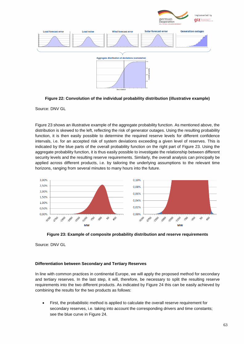
63

Figure 22: Convolution of the individual probability distribution (illustrative example)

Source: DNV GL

Figure 23 shows an illustrative example of the aggregate probability function. As mentioned above, the

distribution is skewed to the left, reflecting the risk of generator outages. Using the resulting probability

function, it is then easily possible to determine the required reserve levels for different confidence

intervals, i.e. for an accepted risk of system deviations exceeding a given level of reserves. This is

indicated by the blue parts of the overall probability function on the right part of Figure 23. Using the

aggregate probability function, it is thus easily possible to investigate the relationship between different

security levels and the resulting reserve requirements. Similarly, the overall analysis can principally be

applied across different products, i.e. by tailoring the underlying assumptions to the relevant time

horizons, ranging from several minutes to many hours into the future.

Figure 23: Example of composite probability distribution and reserve requirements

Source: DNV GL

Differentiation between Secondary and Tertiary Reserves

In line with common practices in continental Europe, we will apply the proposed method for secondary

and tertiary reserves. In the last step, it will, therefore, be necessary to split the resulting reserve

requirements into the two different products. As indicated by Figure 24 this can be easily achieved by

combining the results for the two products as follows:

• First, the probabilistic method is applied to calculate the overall reserve requirement for

secondary reserves, i.e. taking into account the corresponding drivers and time constants;

see the blue curve in Figure 24.

64

• Secondly, the same analysis is carried out for tertiary reserves. Assuming that tertiary

reserves cover a longer time horizon and at least the same drivers as secondary frequency

control, the resulting volumes can be expected to be larger; see the orange curve in Figure

24.

• The effective need for tertiary reserves can then be easily determined as the difference

(orange arrows) between the overall reserve requirements across the timeframe for tertiary

reserves and the volumes already covered by secondary reserves (blue arrow).

As indicated by the green arrow, the resulting volumes can furthermore be compared against a positive

and negative system incident, i.e. in a similar way as for primary frequency control. This may probability

as an additional plausibility check and/or allow to get a better idea about the number of major outages,

which are covered by the resulting reserve requirements18.

Figure 24: Differentiation between secondary and tertiary volumes (illustrative example)

Source: DNV GL

18 In practice, the resulting reserve volumes are usually sufficient to cover multiple simultaneous outages.

Nevertheless, a corresponding comparison may help to gain further insights and facilitate communication of the

method’s results.

0,00%

0,05%

0,10%

0,15%

0,20%

0,25%

0,30%

Pro

ba

bil

ity

Deviation (MW)

Secondary Tertiary

Reference incidents

65

6 Specific Assumptions for Southern Region Grid States

DNV GL has quantified the secondary and tertiary reserve requirements at the state / regional level

using the probabilistic method described in Task 2 (Section 5), considering the 2022 power scenario.

Based on the Government of India’s target of installing 175 GW of RE capacity nationally by the year

2022, we have considered the following five scenarios (compare [60], [61]):

• Status quo 2018

• 70 GW Solar – 45 GW Wind (70S-45W): 72% of the national target achieved

• 100 GW Solar - 60 GW Wind (100S-60W): 100% of the national target achieved

• 60 GW Solar - 100 GW Wind (60S-100W): Solar and wind targets reversed in comparison to

the official target

• 150 GW Solar – 100 GW Wind (150S-100W): Ambitious RE growth.

6.1 Basic Assumptions for Dispatch scenarios and Reserve Dimensioning

Peak load and installed RE capacity

We have considered the installed RE capacity in 2018 and the Government of India’s state-wise break-

up of the 175 GW target to derive the RE capacity for other scenarios in the southern states. Peak load

for 2022 has been considered as per National Electricity Plan – Generation 2017- 22.

Four scenarios have been considered as future scenarios based on the assumptions mentioned above.

The 100S-60W and 60S-100W scenarios are opposite to examine the impact of the high volume of

installed wind capacity versus PV capacity and vice versa. 150S-100W is considered as an ambitious

scenario in terms of RES capacity installation. Moreover, the 70S-45W scenario was suggested as a

moderate scenario for renewable sources installed capacity.

Table 17: Basic scenario assumptions - Installed RE capacity and Peak load

State RE Capacity (MW) Peak Load

Status

quo

2018

70S-45W 100S-60W 60S-100W 150S-100W 2018 2022

Andhra Pradesh 7176 12647 19059 20057 31932 8995 11843

Karnataka 10790 14061 17445 16817 29104 12561 14271

Kerala 139 632 1030 710 1030 4261 5263

Tamil Nadu 10933 17372 24318 27134 39757 19521 20273

Telangana 3720 5549 7956 5596 9547 10410 14499

Total 32758 50262 69808 70314 111370 55748 66149

Source: DNV GL Analysis

Table 18 provides a detailed breakdown of our assumptions on installed wind capacity by state.

66

Table 18: Basic scenario assumptions - Installed wind capacity by state (MW)

STATE NREL Base

Scenario 2015

Status quo 2018

20S-50W 100S-60W

60S-100W

150S-100W

Andhra Pradesh 1,037 4,090 6,755 8,111 13,495 13,495

Karnataka 2,856 4,695 5,166 6,199 10,332 10,332

Kerala

Tamil Nadu 5,790 8,359 9,912 11,891 19,817 19,817

Telangana 0 128 1,679 2,001 3,333 3,333

Total 9,683 17,272 23,512 28,202 46,977 46,977

Source: DNV GL analysis

Table 19 provides the corresponding assumptions for solar plants (PV).

Table 19: Basic scenario assumptions - Installed PV capacity by state (MW)

STATE NREL Base

Scenario 2015

Status quo 2018

20S-50W 100S-60W

60S-100W

150S-100W

Andhra Pradesh 271 3,086 2,185 10,948 6,562 18,437

Karnataka 80 6,096 2,241 11,246 6,485 18,772

Kerala 0 139 230 1,030 710 1,030

Tamil Nadu 160 2,574 2,505 12,427 7,317 19,940

Telangana 73 3,592 1,060 5,955 2,263 6,214

Total 584 15,486 8,221 41,606 23,337 64,393

Source: DNV GL analysis

Table 20 summarises our assumptions on the future development of conventional capacity.

Table 20: Basic scenario assumptions - conventional plants

Andhra Pradesh Karnataka Kerala Tamil Nadu Telangana

Present (MW)

2022 (MW)

Present (MW)

2022 (MW)

Present (MW)

2022 (MW)

Present (MW)

2022 (MW)

Present (MW)

2022 (MW)

Coal 11,590 13,230 9,480 7,760 - - 12,760 13,955 6,682 8,862

Gas & Diesel

4,917 4,917 153 523 694 694 1,238 1,238 - -

Nuclear - - 880 880 - - 2,440 2,940 - -

Hydro 1,262 2,060 4,169 4,415 1,873 1,811 2,086 2,678 2,302 2,301

Biomass 500 500 1,800 1,800 1 1 1,004 1,004 178 178

Total 18,269 20,707 16,482 15,378 2,568 2,506 19,528 21,815 9,162 11,341

Source: National Electricity Plan 2017-22 [62]

Outage rates

As described in Section 5.5, we used the outage statistics from Europe and the U.S. as given in Table

16 and scaled the technology-specific values for India. Using the information from CEA reports [63]

[64], we have calculated the Mean Time To Failure (MTTF) for hydro and thermal power plants shown

in Table 21. The MTTF can be estimated to be 1645 hours. This value is about 1/3 lower than in Western

Europe (2,500 h), which corresponds to an approx. 50% higher outage rate.

67

Table 21: Mean Time to Failure Calculation for Hydropower plants

Determination of MTTF

Number of units 712 Total ‘unit hours’ in year 6,237,120

- Total hours of planned outages in a year 415,488

- Total hours of forced outages in a year 169,962

= Total (potential) operating hours 5,651,670

/ Number of forced outages 3,436

= Mean time to failure (MTTF, in h) 1,645

Source: DNV GL Analysis

For thermal power plants, Forced Outage Rates (FOR) has increased from ~10% in the previous

decade to 19% in 2014-15. Figure 25 demonstrates an overview of the annual performance review of

thermal power stations for 2014-15.

Figure 25: Overview of the annual performance review of thermal power stations for 2014-15

Source: CEA Overview of the annual performance review of thermal power stations for 2014-15

Wind Profiles

DNV GL owns a database – HORNET - where data from most common public sources is stored, namely

MERRA2 and ERA5. Reanalysis is made of these data in order to have a finer mesh of the selected

land going down to a 30km side square mesh. From this mesh, the hourly wind speed and direction of

each node for 19 years (2000-2018). 13 points have been chosen in 4 states (Kerala was excluded),

based on the location of future potential wind farm locations with an acceptable wide variety. Data of

each node has been pondered and weighted and then aggregated to obtain a single representative

hourly wind profile for each state.

68

DNV GL has then used a turbine model representing standard turbine designs to convert the wind

speed data into electric power. By using per unit values, it was then possible to apply these profiles to

the different scenarios considered.

We have chosen different potential locations in each state in order to cover a wide range of areas in

each state and derived one single profile, which represented the wind profile of the states.

Figure 26: Wind potential areas in the Southern region

Source: DNV GL Analysis

Solar Profiles

For the solar resource, PV GIS application from JRC has been used. JRC is the joint research institute

of the European Union that performs studies in all fields to provide independent scientific advice and

support to the EU. Among them, PV GIS, based on satellite data, is able to calculate solar radiation for

the earth's surface with a resolution of about 4km. PV GIS has also the capability to calculate the

optimal angle of the PV panels and can also estimate the electric power output.

For this purpose, different representative locations of each state have been selected. For each of these

regions, the potential hourly generation of 1kWp has been extracted from PVGIS for all years for which

these time series where available, i.e. a period of 11 years (2005-2015). Figure 27 shows a screenshot

of the PVGIS tool.

The potential hourly generation (per kWp) of each of these locations has been multiplied by the capacity

that is expected to be installed for each region. Adding these results, the total hourly generation for

each state is obtained. The last step is to divide the total generation by the total installed capacity in

order to obtain a non-dimensional per unit value that can be applied to different scenarios with different

PV capacity forecasts.

69

Figure 27: PV GIS tool screenshot

Source: JRC –PVGIS

Residual load

The hourly load and VRE profiles were combined to derive a time series for the residual load. For this

purpose, the wind and solar profiles for the years 2005 to 2015 were combined with the scaled load

profile, i.e. the same load profile was applied to all historic VRE time series. For the years 2018 and

2022, all three profiles were scaled to the corresponding scenario assumptions, i.e. based on installed

capacity resp. peak load.

Overall, the analysis under this study has thus been able to rely on 11 years of (synthetic) profiles of

load, wind, solar and residual load.

6.2 Determination of typical dispatch curves and scenarios for assumed

reserve-requirements

We have derived a daily dispatch curve for all ten cases considered. In practice, each dispatch was

developed in an iterative approach based on the available wind and PV power of the days with peak

and low residual load selected in each scenario. Starting from an initial situation, this dispatch was used

for the dimensioning of secondary reserves.

In the first step, two ‘typical’ days were selected for each scenario. For each year, a ‘Low’ and a ‘Peak’

day were chosen, reflecting days with low resp. high residual load; see Table 22. The corresponding

days were chosen from the set of 11 years of residual load profiles (see the previous section) with a

view of ensuring a maximum range of residual load as well as high ramp rates. Ideally, each pair of

selected days should thus ideally cover the entire range between a very low and a very level of residual

load observed for this particular target year, but also contain hours with quickly increasing residual load.

70

Table 22: Structure of selected days

2018 Status

quo

70S-45W 100S-60W 60S-100W 150S-100W

Day with very low

residual load

Status quo

Low

70S-45W

Low

100S-60W

Low

60S-100W

Low

150S-100W

Low

Day with very high

residual load

Status quo

Peak

70S-45W

Peak

100S-60W

Peak

60S-100W

Peak

150S-100W

Peak

Source: DNV GL Analysis

For each of these selected days, an hourly dispatch profile was then derived by using a sequence of

steps and principles for different technologies. These steps can be summarized as follows:

• For wind and solar PV, the initial dispatch was set equal to the relevant profile for the

corresponding day.

• In a second step, hydro pump storage generation and load have been calculated based on the

maximum available energy (maximum power for 8 hours) and remaining residual load. Smaller

hydro storage units have been assumed as must-run units in every hour of the day.

• Any remaining need for a generation was then assigned to individual units according to the

merit order. The schedule of dispatchable thermal units (Nuclear, lignite, and coal) was then

derived from the same day based on the remaining residual load, minimum, and maximum

available power, which has been assumed as a percentage of max power and been

constrained manually for each scenario respectively. Larger hydro storage units and CCGT

that have been considered as dispatchable units then would cover the load if it is necessary.

• In case of remaining load, the GT and diesel were the next technologies to be dispatched and

in case of peak load scenarios and the necessity for import from other regions the remaining

residual load was assigned to import. Furthermore, in low load scenarios, the additional

generation (in case of exceeding the demand) is considered as export to other regions.

In the following, we briefly present the resulting dispatch schedules for the ten cases.

Status quo 2018 scenarios

The availability of solar energy is significant in peak load scenario than the low residual load scenario,

while the wind power availability considerably increases in low residual load scenario. The output of

non-dispatchable plants and dispatchable thermal plants basically corresponds to the schedule from

the selected days, with 90% constraint as for coal and nuclear generation and 38% availability of hydro.

It should be mention that Monsoon conditions have been imposed on the must-run hydro units with a

factor of 10%. The difference between load and total generation considered as import/export from other

regions. Figure 28 shows the status quo 2018 peak and low scenarios dispatch, load, residual load and

required hourly import/export from other regions.

71

Peak Low

Figure 28: Assumed dispatch for Status quo 2018 scenarios

Source: DNV GL analysis

70S-45W scenarios

Figure 29 illustrates the dispatch of different sources (conventional, hydro and RES) with hourly load,

residual load and import/export of two future days in the 70S-45W scenario. The installed capacity of

this scenario is more moderate than the other ones. This explains the need for higher import values in

the peak load case and lowers export quantities during the daytime (during high availability of RES

power) in low load case.

Peak Low

Figure 29: Assumptions dispatch 70S-45W

Source: DNV GL analysis

100S-60W scenarios

The dispatch in future scenarios was optimized with a similar approach in 2018 with considering future

thermal, hydro and renewable (wind and solar) capacities. Individual units are allowed to be operated

at up to 95% of capacity in the peak and 90% in the low demand case19

Figure 30 shows two days from a 100S-60W scenario with high and low load demand. Generation by

VRE reduces the usage of dispatchable coal and hydro. In case of the low residual demand scenario,

the decentralized plants, thermal and hydro must-run generation and there would be a possibility of

19 The 90% limit was chosen based on a simplified analysis of the ratio between scheduled loading and

synchronous capacity of all committed plants in the year 2018, which showed that most plants were very seldom

dispatched at their maximum.

72

power export to other regions up to 11500 MW per hour during the daytime, due to high availability of

RES (especially solar, as it has a more installed capacity in this scenario and then the wind power).

The daily volume of energy available from solar PV is not comparable in both cases. In contrast, the

charts show a marked difference with regards to the expected output of wind power, i.e. whilst the peak

case is based on a day with limited speeds, whilst wind speeds are much higher in the Low case.

Peak Low

Figure 30: Assumptions dispatch for 100S-60W scenarios

Source: DNV GL analysis

60S-100W scenarios

Compare to the 100S-60W scenario 60S-100W scenario has more installed wind power than the PV in

the future. Figure 31 demonstrates two sample future days with peak and low residual load. The units

in this scenario are a constraint to 90% in both low and peak cases. Considering existing must run

units, dispatchable generation and accessible RES, import from other regions will be essential for peak

load case while taking low load case conditions into account almost 15000 MW export would be

possible in some hours during the daytime. As it was mentioned before, high wind power availability

occurs in low residual load scenario and the fact that this scenario contains less installed PV capacity

than the last one can somewhat justify the necessity for import of power in peak load case.

Peak Low

Figure 31: Assumptions dispatch for 60S-100W scenarios

Source: DNV GL analysis

73

150S-100W scenarios

Figure 32 demonstrates two sample future days from a 150S-100W scenario with high and low load

demand. In this scenario, more renewable capacities are installed. Consequently, there is even more

RES power available, whilst the system still faces various must-run / minimum load constraints of

conventional units. As a result, one can again observe substantial export values, due to VRE during

the day.

In this case, the Low case shows high wind speeds and high PV power generation due to the significant

amount of installed PV.

Peak Low

Figure 32: Assumptions dispatch 150S-100W

Source: DNV GL analysis

74

7 Results of Dimensioning Calculations for Southern Region

7.1 Basic results (secondary and tertiary reserves) Based on the scenario assumptions and simplified dispatch situations provided in Section 6.1 and

Sections 6.2, hourly reserve requirements are calculated for Southern region states using the

methodology described in section 5. In addition, the following assumptions have been applied with

regards to the applicable timescales:

• Secondary reserves have been dimensioned to cover a timescale of 30 minutes (0.5 hours).

• Tertiary reserves have been dimensioned to cover variations up to 2 h ahead, minus the

share already covered by secondary reserves.

Status quo 2018 scenarios

Figure 33 shows the secondary reserves required for the southern region for the Status quo 2018 peak

and low scenarios. Calculations are based on a timescale of 0.5 hours ahead and an accepted risk

margin of 0.1%, i.e. a confidence interval of 99.9%.

During night hours in the status quo peak scenario, the total reserve requirement is majorly driven by

the conventional plant outage since the VRE is considerably less. Hence, a flat profile of the total

reserves during night hours can be observed.

During daytime in the status quo peak scenario, the total reserve requirement increases by almost

1,000 MW due to risk related to VRE forecast error. The production by VRE replaces conventional

generation and therefore reduces the dispatch of conventional generation. Hence, the risk of

conventional generation outages drops, although it is partially outweighed by the increase in forecast

inaccuracy from VRE. So, a nearly flat profile during the daytime can be observed in the regional

reserve requirement in the low scenario. The reserve requirement profile is fluctuating in the low

scenario more than the peak scenario during night hours due to the availability of wind.

Peak Low

Scenario Lead time Forecast quality Outage rates Risk margin Adapt. forecast

Status quo

2018 0.5 &1&2 h 100% 250% 0.1% Yes

Figure 33 Regional Secondary Vs Tertiary reserves for Status quo 2018

Source: DNV GL analysis

75

70S-45W scenarios

Figure 34 shows the secondary reserves required for the southern region for the 70S-45W scenario.

With additional RE in 70S-45W from the status quo, the reserve requirement has increased in low and

peak scenarios. During night hours in peak scenario, a flat profile of the total reserves during night

hours can be observed since the VRE is considerably less. While during daytime in peak scenario, the

reserve requirement is fluctuating due to the cumulative effect of VRE forecast error, load forecast error,

and conventional plant outages.

During daytime in the low scenario, similar to the status quo, the risk due to VRE forecast error gets

nullified by the reduced dispatch of conventional generation. Hence a flat profile of reserve requirement

can be observed.

Peak Low

Scenario Lead time Forecast quality Outage rates Risk margin Adapt. forecast

70S-45W 0.5 &1&2 h 100% 250% 0.1% Yes

Figure 34: Regional Secondary Vs Tertiary reserves for 70S-45W

Source: DNV GL analysis

100S-60W scenarios

Figure 35 shows the secondary and tertiary reserves requirements for the 100S-60W peak and low

residual load scenario. Compared to the Status quo 2018 scenario, the secondary reserve requirement

for states and region shows drastic variations in the 100S-60W peak scenario during the daytime. The

initial increase in the secondary reserve requirement during the day can be explained by the increase

in solar forecast error. Since the generation by VRE reduces the usage of dispatchable coal and hydro

which reduces the risk due to conventional plant outage, a subsequent decrease in reserve requirement

in peak scenario can be observed.

76

Peak Low

Scenario Lead time Forecast quality Outage rates Risk margin Adapt. forecast

100S-60W 0.5 &1&2 h 100% 250% 0.1% Yes

Figure 35: Regional Secondary Vs Tertiary reserves for 100S-60W Scenario

Source: DNV GL analysis

60S-100W scenarios

Compared to the previous scenario, 60S-100W has less installed photovoltaic and more wind power. This leads to lower secondary reserve as well as a lower required tertiary reserve during the daytime in case of peak residual load.

Peak Low

Scenario Lead time Forecast quality Outage rates Risk margin Adapt. forecast

60W-100S 0.5 &1&2 h 100% 250% 0.1% Yes

Figure 36: Regional Secondary Vs Tertiary reserves for 60S-100W

Source: DNV GL analysis

150S-100W scenarios

Figure 37 shows the secondary and tertiary reserve requirements for the 150S-100W peak and low

residual load scenario. With the increasing penetration of VRE and a corresponding reduction in the

share of conventional generations, reserve requirement becomes increasingly symmetrical. The VRE

forecast error becomes the major driving factor for reserve requirement and the risk related to the

conventional plant outage becomes very less.

77

In the peak scenario, the secondary reserve requirement is almost steady during night time which can

be attributed to very low VRE and the major driving factor will be conventional plant outage. Hence, the

secondary reserve requirement calculated as per the deterministic approach almost matches with the

probabilistic approach during night hours. In the low scenario, the amount of secondary reserve

requirement increases due to high VRE. During night hours, the driving factors are risks related to

conventional plant outage and wind forecast error. In contrast, because of high PV power penetration

during the day, the demand for reserve increases, however due to a significant drop in wind power

availability during the midday, the required reserve decreases. In other words, a high proportion of

power from renewable energy sources in the system leads to the higher required reserve.

Peak Low

Scenario Lead time Forecast quality Outage rates Risk margin Adapt. forecast

150S-100W 0.5 &1&2 h 100% 250% 0.1% Yes

Figure 37: Regional secondary vs. tertiary reserves for 150S-100W

Source: DNV GL analysis

7.2 Potential benefits of regional sharing

Status quo 2018 scenarios

Figure 38 gives an overview of the total secondary and tertiary reserves at the state and regional level.

As per the present deterministic approach, the sum of secondary and tertiary reserves to be kept at the

regional level is more than the proposed probabilistic approach in most of the hours. For the total

upward reserves, dimensioning at the regional level is beneficial rather than at individual states. But,

the total downward reserves at the regional level is almost the sum of individual states.

78

Status Quo 2018 Peak Status Quo 2018 Low

Scenario Lead time Forecast quality Outage rates Risk margin Adapt. forecast

Status quo 2018 2h 100% 250% 0.1% Yes

Figure 38: Sum of secondary and tertiary reserve vs. regionally required reserves, status quo 2018 scenario

Source: DNV GL analysis Figure 39 shows the secondary reserves required for the southern states and region for Status quo

2018 peak and low scenarios. It is perceivable, that the sum of states’ upward secondary reserves

exceeds 3,000 MW, while the required secondary reserves for southern region (consider all states as

one large region) hardly reaches 1,500 MW during the day in case of peak residual load, this effect is

less noticeable in low residual load scenario especially during the midday. On the contrary, the sum of

state-wise downward secondary reserve in both low and peak scenarios is almost equal to the regional

required downward secondary reserve.

79

Status Quo 2018 Peak Status Quo 2018 Low

Scenario Lead time Forecast quality Outage rates Risk margin Adapt. forecast

Status quo

2018 0.5h 100% 250% 0.1% Yes

Figure 39: Secondary reserve requirements for status quo 2018 with 0.5 h timescale

Source: DNV GL analysis

100S-60W scenarios

100S-60W includes more RES installed capacity than the 2018 status quo scenario, consequences of

which can be clearly seen in Figure 40, where the secondary and tertiary reserves at regional and state

levels with different timescale are illustrated. The impact of renewables is more tangible during the

daytime, when the PV power highly influence the RES availability.). A difference that can be seen

between the 2018 status quo and 100S-60W scenarios calculated total secondary and tertiary reserves,

is the required regional total reserve (sum of 2ry and 3ry reserves). In case of additional future RES

capacities, the sum of reserves in region level would be closer to the sum of reserves in five states,

exclusively during the high RES availability.

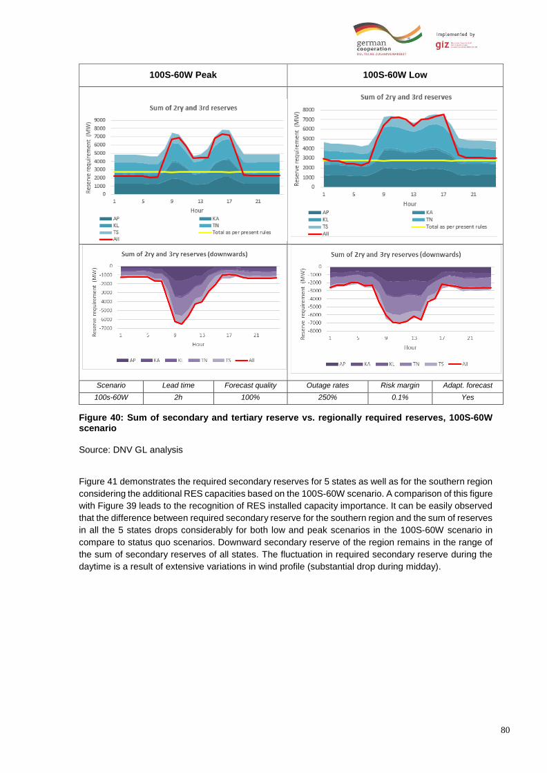
80

100S-60W Peak 100S-60W Low

Scenario Lead time Forecast quality Outage rates Risk margin Adapt. forecast

100s-60W 2h 100% 250% 0.1% Yes

Figure 40: Sum of secondary and tertiary reserve vs. regionally required reserves, 100S-60W scenario

Source: DNV GL analysis Figure 41 demonstrates the required secondary reserves for 5 states as well as for the southern region

considering the additional RES capacities based on the 100S-60W scenario. A comparison of this figure

with Figure 39 leads to the recognition of RES installed capacity importance. It can be easily observed

that the difference between required secondary reserve for the southern region and the sum of reserves

in all the 5 states drops considerably for both low and peak scenarios in the 100S-60W scenario in

compare to status quo scenarios. Downward secondary reserve of the region remains in the range of

the sum of secondary reserves of all states. The fluctuation in required secondary reserve during the

daytime is a result of extensive variations in wind profile (substantial drop during midday).

81

100S-60W Peak 100S-60W Low

Scenario Lead time Forecast quality Outage rates Risk margin Adapt. forecast

100S-60W 0.5h 100% 250% 0.1% Yes

Figure 41 Secondary reserve requirements for 100S-60W with 0.5 h timescale Source: DNV GL

analysis

Source: DNV GL analysis

150S-100W scenarios

Figure 42 illustrates the total secondary and tertiary reserves in states and the regional level. As per

the present deterministic approach, the total amount of secondary and tertiary reserves at the regional

level is close to the proposed probabilistic approach during the daytime. A brief comparison between

the previous scenarios and the 150S-100W scenario would emphasize on the impact of RES proportion

in the system. The difference between the sum of reserves at regional level and the sum of secondary

and tertiary reserves of all 5 states in various scenarios, does not change significantly during the dark

hours, especially in case of the low residual load. In contrast, this variation decreases as the RES

capacity in the system increases.

82

150S-100W Peak 150S-100W Low

Scenario Lead time Forecast quality Outage rates Risk margin Adapt. forecast

150S-100W 2h 100% 250% 0.1% Yes

Figure 42: Sum of secondary and tertiary reserve vs. regionally required reserves, 150S-100W scenario

Source: DNV GL analysis 150S-100W has the highest proportion of RES among all the scenarios. This results in a large amount

of required secondary reserve in each hour and much less difference between the sum of states’

secondary reserves and the regional requirement for secondary reserve than the previous scenarios.

Figure 43 shows the upward and downward secondary reserves in peak and low residual load cases

in the 150S-100W scenario. As it can be recognized, the sum of secondary reserves of 5 states (AP,

KA, KL, TN, TS) during the daytime (when RES has a higher penetration proportion in the system) is

approximately equal to the regional secondary reserve requirement. In contrast, during dark hours, the

sum of state-wise secondary reserves is almost three times larger than the required reserve for the

southern region.

Graphs regarding 70S-45W and 60S-100W scenarios are available in Appendix A. Overview of results

for 70S-45Wand Appendix B. Overview on results for 60S-100W respectively. It should be mentioned

that the general trend of the graphs is similar to the previously analyzed scenarios, however, the values

vary based on the amount of installed capacity in each scenario.

Graphs regarding the status quo 2018 scenario and 150S-100W scenario with a confidence level of

99.50% and outage rate of 150% are available in Appendix C - Overview on results with Confidence

Level of 99.50% and Outage rate of 150%. The quantum of reserve required depends on the risk margin

and outage rate of conventional sources. This illustrates that reserve requirements with confidence

83

Level of 99.50% and outage rate of 150% will be ~2000 MW lesser compared to the reserve

requirements with a confidence level of 99.90% and outage rate of 250%.

150S-100W Peak 150S-100W Low

Scenario Lead time Forecast quality Outage rates Risk margin Adapt. forecast

150S-100W 0.5h 100% 250% 0.1% Yes

Figure 43 Secondary reserve requirement for 150S-100W

Source: DNV GL analysis

7.3 Sensitivity to key assumptions and developments

Comparison between different scenarios

Figure 44 summarizes the calculated secondary reserve requirements for all low scenarios. The

calculations are based on a timescale of one hour ahead and an accepted risk margin of 0.1%, i.e. a

confidence interval of 99.9%. The results for the year 2018 range between approx. 1,500 to 2,500 MW.

2018 requirements are dominated by the need for upward regulation, reflecting outage risks.

On the contrary, volumes for future scenarios increase, especially during daytime and the scenarios

with high solar power penetration in the system. This trend mainly reflects the risk of VRE forecast

errors, in particular, solar PV. Conversely, the need for additional reserves is considerably less during

night hours where it is largely dependent on conventional unit outages and is somehow driven by wind

power (for low scenarios when the wind availability is much higher than the peak scenarios). Since the

future installed capacity of wind and solar varies based on the scenario, the required reserve is

considerably diverse in different scenarios, especially during the daytime. This illustrates that future

reserve requirements are primarily influenced by the predicted output of wind (or solar) power on a

given day. while in the daytime both downward and upward reserves vary around 6,000 MW from

scenario status quo 2018 to scenario 150S-100W (the scenario with highest RES capacity), there will

be less than 2,000 MW difference in the dark-time between the same mentioned scenarios.

84

Upward secondary reserve Downward secondary reserve

Scenario Lead time Forecast quality Outage rates Risk margin Adapt.

forecast

See legend 1 hour 100% 250% 0.1% Yes

Figure 44: Calculated secondary reserve requirements (1-hour timescale)

Source: DNV GL analysis

Different time horizons

To assess the impact of short-term forecast errors, Figure 45 presents an overview of the necessary

reserve requirements when trying to cover VRE and other forecast errors over different time horizons,

i.e. from 0.5 till 8 hours ahead. Not surprisingly, this chart reveals major variations, i.e. required reserves

increase during peak hours increase.

Upward secondary reserve Downward secondary reserve

Scenario Lead time Forecast quality Outage rates Risk margin Adapt. forecast

100S-60W See legend 100% 250% 0.1% Yes

Figure 45: Calculated secondary reserve requirements (Different timescale)

Source: DNV GL analysis

Impact of forecast accuracy

One of the key drivers for future requirements will be the accuracy of VRE forecasts. Our basic

calculations are based on the assumption that future forecast errors will be similar to the accuracy

currently achieved in Spain or Eastern Germany. However, the accuracy of VRE has increased

considerably over the past decade. Between the mid-2000s and 2014, the hour-ahead wind forecast

85

error in Germany decreased from about 1.5% to less than 1% [59]. Similarly, Figure 46 shows continued

improvements for a large German portfolio in the period 2013 to 2016. Besides methodological

improvements, one of the key enablers of such developments has been the access and use of sufficient

measurement data, which have become available as the penetration of VRE increased. It seems

reasonable to assume that this will also be the case in India.

Figure 46: Improvements of forecasting accuracy (example of large German portfolio)

Source: [59]

To test the potential impacts, we have run another sensitivity in which we have varied the quality of

load and VRE forecasts. Figure 47 shows the relationship between different forecast errors and the

need for secondary frequency control with a timescale of one hour ahead and assumptions regarding

the 100S-60W- low scenario. If India resp. southern region improved forecast accuracy by about 25%

in the future, reserve requirements would decrease for upward regulation, with a potential for future

reductions in case of further improvements. Conversely, decreasing forecast quality by 50% might

require a considerable amount of additional reserve.

This highlights the importance of forecast quality in systems with a high penetration of VRE as these

reductions would likely allow for significant cost savings as a result of a more economic generation

dispatch.

Upward secondary reserve Downward secondary reserve

Scenario Lead time Forecast quality Outage rates Risk margin Adapt. forecast

100S-60W 1 hour See legend 250% 0.1% Yes

Figure 47: Calculated secondary reserve requirements (Different forecast accuracies)

Source: DNV GL analysis

86

Impact of outage rates

Different outage rates have a minor impact on the calculated secondary control. For this purpose, we

have tested another sensitivity in which outage rates have been changed by ±1/3 of the current values,

which are about 50% higher than typical outages rates in Central Europe.

Figure 48 demonstrates that reserve requirements basically remain constant, i.e. there is no tangible

difference between the different curves. This finding complies with our earlier observation that outages

have a limited impact on probabilistic requirements for secondary reserve. Whilst this observation may

seem surprising at first sight, it can be explained by the limited timescale for secondary reserve.

Consequently, the results reflect the same combination of outages. In other words, the change of

assumptions does not suffice to result in more or less simultaneous outages being relevant. However,

the impact of outages can be seen during the dark hours when there would be less proportion of

renewables in the system and conventional power plants are playing a more influential role in the

system.

Upward secondary reserve Downward secondary reserve

Scenario Lead time Forecast quality Outage rates Risk margin Adapt. forecast

100S-60W 1 hour 100% See Legend 0.1% Yes

Figure 48: Calculated secondary reserve requirements (Different outage rates)

Source: DNV GL analysis

Accepted risk margins

The reserve requirements presented above are based on an accepted risk margin of 0.1%. This implies

that the resulting volumes should be enough to ensure sufficient reserves in 99.9% of all hours, i.e.

accepting a deficit in up to 9 h per annum on average. This requirement corresponds to the criteria

applied in Germany, whereas for instance the Austrian (APG) and Belgian (Elia) TSOs apply a lower

threshold of 99%.

Accepting a slightly higher risk margin may lead to a significant decrease in reserve requirements as

illustrated by Figure 49. Conversely, stricter confidence intervals will lead to even higher reserve needs.

This observation highlights the conflicting objectives of ensuring system security, on the one hand, and

minimizing costs, on the other hand. As the difference between the criteria applied by Germany as

opposed to Austria or Belgium show, this criterion ultimately represents an arbitrary choice.

Nevertheless, it should be noted that these TSOs can always rely on the inherent support by a large

synchronous system.

87

The results shown below are based on a time horizon of one hour ahead and assumptions regarding

the 100S-60W- low scenario.

Upward secondary reserve Downward secondary reserve

Scenario Lead time Forecast quality Outage rates Risk margin Adapt. forecast

100S-60W 1 hour 100% 250% See legend Yes

Figure 49: Calculated secondary reserve requirements (different risk margins)

Source: DNV GL analysis

88

8 Benefits of reserve sharing

8.1 Principal options

Reserve sharing may take different forms and serve different purposes. As illustrated by Table 23, we

differentiate between four principal approaches, which reflect two different dimensions as follows:

• Area of envisaged savings, i.e. with regards to the holding of reserves as opposed to the real-

time activation of balancing energy,

• Means of achieving such savings, i.e. either through a reduction of volumes by pooling of

needs vs. reducing costs through the coordinated use of available resources.

The first dimension corresponds to the need of holding sufficient reserve available, on the one hand,

and the actual use of the corresponding services in real-time. Conversely, the second dimension

differentiates between measures aimed at reducing the required volume of such services as opposed

to approaches for using the least expensive resources available.

We emphasise that the four basic options shown in Table 23 are principally independent of each other.

For instance, the coordinated procurement of reserves does not necessarily require a coordinated

approach for real-time activation and vice versa. Similarly, present arrangements for primary,

secondary and tertiary reserves in India involve some elements of joint dimensioning and reserve

sharing, but without imbalance netting. Conversely, a group of Central European countries applies

implemented imbalance netting without joint dimensioning (compare section 8.2.3). Likewise, European

TSOs are currently engaging in several projects for facilitating the mutual exchange of balancing

services in real-time in Europe (see section 8.2) without requiring the implementation of any of the other

options.

In the following, we briefly introduce the four principal concepts, before section 8.2 presents selected

illustrative examples from Europe. To assess the potential impact and benefits for the Southern region,

we derive quantitative assessments for each of the four different approaches in section 8.3. Finally,

section 9 comments aspects to be considered in case of implementation.

Table 23: Principal options for reserve sharing

Source: DNV GL

Joint dimensioning / Sharing of reserves

Under joint dimensioning, reserve requirements are determined for the combined area of two or more

control areas, rather than for each control area separately. As already illustrated under Task 3, joint

dimensioning allows reducing overall reserve volumes as reserve requirements for a single large area

are typically less than the sum of the individual needs of several sub-zones. Indirectly, joint reserve

dimensioning thus also allows for cost savings as less reserves need to be held available.

Area of savings Type of savings

Pooling of needs Pooling of resources

Reserves (MW)Joint dimensioning /

Sharing of reserves

Joint procurement /

Sharing of offers

Holding of reserves to

enable real-time balancing

Real-time

balancing (MWh)Imbalance netting

Joint procurement /

Sharing of offers

Activation of energy for

real-time balancing

Reduces volumes to be

procured / held available

Improved sourcing reduces

specific costs

89

By definition, joint reserve dimensioning requires some form of mutual assistance between the

participating system operators, i.e. they need to at least partially ‘share’ reserves amongst each other.

As it is hardly possible to define exactly how much each individual system contributes to overall savings,

total benefits are usually shared between all participating system operators according to some simple

measures, such as by a proportional distribution of overall reserves requirements (or savings) overall

systems.

Actual savings generated by joint reserve dimensioning depend on several factors. As the analysis

under task 3 has shown, savings are particularly large in systems or situations where reserve needs

are primarily driven by generator outages, due to the limited degree of simultaneity. Conversely, the

benefits of reserve sharing in systems dominated by variable RE primarily depend on the spatial

correlation of VRE forecast errors and variability.

Imbalance netting

Whilst reserve dimensioning aims at reducing the volume of reserves to be held available, imbalance

netting has the aim of minimizing the actual use or activation of reserves. Similar to the concept of

probabilistic reserve dimensioning, this approach is based on the fact that a considerable share of real-

time system deviations is of a stochastic nature and that there only is a limited degree of correlation

between simultaneous system deviations of different control areas.

Consequently, this approach aims to prevent the activation of simultaneous control reserve in opposite

directions. This is achieved by real-time ‘netting’ of system imbalances through appropriate control

mechanisms. In practice, system operators “pool” their system deviations, such that the activation of

power and energy from reserves can be limited to the residual net deviation of the entire region. Similar

to the concept of joint reserve dimensioning, this approach focuses on a reduction of physical volumes,

which in turn leads to corresponding cost savings.

Joint procurement / Sharing of offers

As shown by Table 23, system operators may also try to reduce the costs of reserves and real-time

system balancing by ‘pooling’ available resources. As already stated above, this option can be equally

but independently applied for the holding of reserves as well as for real-time activation of reserves. In

contrast to pooling of needs, the exchange and/or joint use of available resources are directly aimed at

cost reduction, i.e. by means of facilitating access to the least expensive resources available. If the

corresponding services are procured and activated through market-based mechanisms, this approach

may also reduce costs by increasing competition between service providers in the whole region.

Based on (European) practices, one can identify three different types or ‘stages’ for a coordinated procurement and/or use of reserves; see Table 24:

• In the SO-Actor model, the local SO may procure services from resources located in external

control areas on a direct contractual basis, i.e. without any direct involvement of the SO of the

external control area. Conceptually, this corresponds to the creation of several parallel ‘market’

in the region, where each SO procures and activates its own needs independently, whilst

service providers may select to which SO(s) to offer their services.

• In case of a common merit order, all available resources within the entire region are combined

into a single ‘pool’ or merit order, and all SOs procure and/or activate necessary services from

this common pool.

90

• The second model represents a somewhat looser form of coordination. In this case, each SO

has exclusive access to all available resources within its own control area. However, SOs

exchange any ‘unused’ or ‘excess’ capacities between others. SOs of control areas with

relatively expensive resources may thus gain access to cheaper options from other areas.

As Table 24 shows, all of the three approaches have been, or are being used in different parts of Europe; some of them are also presented in section 8.2 below.

Table 24: Joint procurement of reserves options

Source: DNV GL

Table 24 also highlights some of the key advantages and drawbacks of each of the three models. As

already stated above, the SO-Actor model effectively creates several separate mechanisms or markets,

especially if individual resources can only be made available to one SO at a time. Whilst this may allow

for increasing competition and cost savings, these benefits are limited or at least at risk due to the

fragmentation of the overall needs or market. In addition, the activation of resources from external

control areas creates certain challenges for real-time scheduling and operation of AGC, as also

discussed in section 4.

These risks and issues can be avoided in case of a common merit order, which by definition represents

the most economic approach in terms of resource use. Nevertheless, it also requires close coordination

and a high degree of harmonisation. Besides the use of similar ‘standard’ products, harmonisation of

also required with regards to pricing and settlement. Furthermore, special rules and mechanisms may

be required to deal with potential congestion.

These challenges are slightly less pronounced when limited cooperation to an exchange of unused

resources. In particular, this reduces complexity in terms of product harmonisation and congestion

management, whereas issues may still arise with regards to pricing and settlement. But similarly,

restricting the share of sharing may also decrease economic benefits.

8.2 Illustrative examples from Europe

To better illustrate the principal models introduced above, this section presents an overview of relevant

projects and initiatives from Europe, as well as an illustrative example for each of the four different

approaches. Table 25 gives an overview of existing and planned projects in Europe. It shows that

Model SO-Actor model Exchange of uncontracted capacities

Common merit order

Key features

- System operator may directly procure services from external service providers (and v.v.)

- Local SO makes ‘excess’ resources/offers available to other SOs

- All SOs procure from common merit order

Examples

- Germany, France (past) - England-France Interconnector

- Local ‘core share’ in some regions using common merit order

- India: RRAS, 1ry

, 2ry

- Germany / GCC

(1ry

/ 2ry

/ 3ry

)

- Central Europe (1ry

)

- Nordic markets (partially)

Pros and cons

- Risk of fragmentation

- Challenges for real-time scheduling and AGC operation

- Requires close coordination

- Similar to common merit order with local priority

- Most economic approach

- Requires close cooperation and harmonised ‘market rules’

91

European TSOs have successfully implemented corresponding mechanisms in all four categories,

whilst three projects are currently underway for facilitating the real-time exchange of balancing services.

It is also visible that most projects focus on exchanges available resources, whereas joint reserve

dimensioning and imbalance netting are still limited to two projects each.

Table 25: Overview of projects ‘reserve sharing’ in Europe

Joint dimensioning

Exchange of reserves

Imbalance Netting

Exchange of balancing services

Existing projects

GCC1 GCC1 GCC1 GCC1

IGCC3 (IGCC)3

FCR4

RPM2 RPM2

Planned projects

MARI5

TERRE6

PICASSO7

1 - Grid Control Cooperation in Germany; 2 - Regulating Power Market in Nordic countries (DK, FI, SE, NO); 3 - International Grid Control Cooperation in Central Europe; 4 - Frequency containment reserves (primary reserves); 5 - Manually Activated Reserves Initiative (MARI); 6 - Trans European Replacement Reserves Exchange (TERRE); 7 - Platform for the International Coordination of Automated Frequency Restoration and Stable System Operation (PICASSO)

Source: DNV GL

Without going into detail, the key characteristics of the individual projects presented in Table 25 can be

summarised as follows:

• The Grid Control Cooperation (GCC), which is presented in more detail in section 8.2.1,

covers the four German control areas and combines cooperation in all categories

• The International Grid Control Cooperation (IGCC) (compare sections 8.2.3 and 8.2.4) has

been developed as a less ambitious form of GCC. It is currently limited to real-time activation

of secondary frequency control but has been gradually expanded to 11 TSOs in 8 European

countries.

• The Regulating Power Market (RPM) in the Nordic countries (Denmark, Finland, Norway, and

Sweden), which covers the joint procurement and use of tertiary reserves, represents the first

example of cross-border integration as it was implemented in the early 2000’s already.

• In Central Europe, nine TSOs from six countries have implemented a mechanism for the joint

procurement of frequency containment reserves (primary reserves), which is presented in

section 8.2.2.

• The ‘Manually Activated Reserves Initiative’ (MARI) was established in 2017 to create a

common European platform for the real-time exchange of balancing energy from tertiary

reserves. Due to the diversity of product definitions, procurement, pricing and settlement rules

in Europe, much of the work under this project focuses on the harmonization of balancing

energy products and trying to ensure the financial neutrality of TSOs. MARI, which is scheduled

to go live in 2022 covers 25 TSOs from almost all European countries (see Figure 50).

92

Figure 50: Members and observers of the European MARI initiative

Source: ENTSO-E (https://www.entsoe.eu/network_codes/eb/mari/)

• The ‘Trans European Replacement Reserves Exchange’, or TERRE, is a cooperation

project of 9 European TSOs (see Figure 51) established in 2016. It aims at creating a common

IT platform and framework for exchanging so-called ‘replacement reserves’ (slow tertiary

reserves) in accordance with the EU Guideline on Electricity Balancing (EBGL). Following

approval of the Replacement Reserves Implementation Framework (RRIF) by the national

regulators in December 2018, the project is currently in the final stages of implementation and

shall go live by the end of 2019.

Figure 51: Members and observers of the European TERRE initiative

Source: ENTSO-E (https://www.entsoe.eu/network_codes/eb/terre/)

• PICASSO stands for the ‘Platform for the International Coordination of Automated

Frequency Restoration and Stable System Operation’. Similar to the corresponding part of

the German GCC, it shall develop and implement a framework for a common merit order for

secondary frequency control, including operation of a real-time IT platform. The project was

originally started by eight TSOs from five countries in Central Europe in 2017, but its

93

membership covers 16 TSOs from 13 European countries; see Figure 52. The TSOs aim to go

live with the aFRR platform by 2020.

Figure 52: Members and observers of the European PICASSO initiative

Source: ENTSO-E (https://www.entsoe.eu/network_codes/eb/picasso/)

8.2.1 Joint reserve dimensioning – GCC in Germany

The grid control cooperation (GCC) was first implemented by the four German TSOs in 2009/2010. As

illustrated by Figure 53, it includes a total of four modules, which jointly aim for a comprehensive

framework for the coordinated dimensioning, procurement and use of secondary and tertiary reserves,

including real-time balancing. To key features of GCC were a transition from separate dimensioning by

each TSO to a single national value (using a common methodology) and joint procurement and

activation of secondary reserves by all 4 TSOs. The methodology for common reserve dimensioning

used to be similar to the approach applied under Task 3 but was changed in late 2018.

94

Figure 53: Grid Control Cooperation functional modules

Source: DNV GL

The transition to joint dimensioning significantly lowered the aggregate demand for secondary (and

tertiary) reserves as shown by the left chart in Figure 54, i.e. with approx. 30% reduction of the need for

upward regulation (from 3,000 to 2,000 MW). In combination with a set of other measures, notably

including increasing forecasting quality and facilitation of the intra-day market, the Germany TSOs have

furthermore been able to maintain their reserve needs at this level, despite a more than three-foiled

growth of wind and solar PV from about 30 GW in 2010 to more than 90 GW in 2016.

Evolution of secondary reserve requirements

between 2008 and 2017 Correlation between total reserve requirements and

penetration of variable RE

Figure 54: Impact of joint reserve dimensioning on total reserve requirements in Germany

Sources: Left - Bundesnetzagentur; Monitoring report 2018; Right - Lion Hirth, Balancing power 2015

– Insights to the German market for balancing power

8.2.2 Joint procurement of frequency containment reserves in central Europe

The project for the common procurement of so-called frequency containment reserves (FCR), e.g.

primary control reserves. The FCR consortium was founded in 2016 and now includes ten TSOs from

seven countries; see Figure 55. Within the FCR Cooperation, primary reserves are procured through a

common merit order list where all TSOs pool the offers they have received. Conversely, all interactions

between balancing service providers (BSPs) and TSOs and BSPs are handled on a national basis.

95

Figure 55: Countries involved in common procurement of FCR

Source: APG

The principle of the common merit order list is illustrated in Figure 56 and Figure 57. In the absence of

congestion, all offers received by the TSOs are pooled into a single merit order. The TSOs then accept

the cheapest offers until the total requirement for primary reserves is met (see Figure 56). This results

in a common marginal price, which is then applied to all accepted offers and the TSOs of all countries.

Figure 56: Marginal price-setting without any congestions

Source: APG

In case this initial matching leads to a violation of a country's import or export capacity, this country is

excluded from the common merit order and a local marginal price is determined for this country only

based on the local offers. For illustration, Figure 57 shows the same example as before but now

assuming that Switzerland hits its export limit. As a result, all offers from Switzerland that are exceeding

available export capacity are rejected and the resulting deficit is covered by accepting one or more offers

from the rest of the region, in this example from the Netherlands. As a consequence, the marginal price

for the region increases. In contrast, the local marginal price for Switzerland decreases as it is now is

determined by the most expensive awarded offer accepted in Switzerland.

Until recently, the FCR mechanism was based on weekly tenders. Since the 1st of July 2019 (delivery

date) daily tenders are used, and for 2020 separate procurement for several time blocks per day is

foreseen.

96

Figure 57: Changes in marginal price in case of congestion (Export limitation)

Source: DNV GL, based on APG

8.2.3 Imbalance Netting in the International Grid Control Cooperation (IGCC)

After the concept of ‘imbalance netting’ had originally been introduced for secondary reserves in

Germany (see section 8.2.1 above), it was extended to other countries in the form of the International

Grid Control Cooperation (IGCC) in 2011. Since then, IGCC has grown to 20 members, with 13 TSOs

from ten countries participating in IGCC operations at present.

Figure 58: Member countries of IGCC

Source: ENTSO-E (https://www.entsoe.eu/network_codes/eb/imbalance-netting/)

Under IGCC, each TSO continues to operate its own load-frequency control (LFC) for secondary

frequency control within its own control area. Nevertheless, whilst secondary frequency control has

traditionally been used to correct the local power imbalance, IGCC has introduced an interim step,

whereby the system imbalances of all participating control areas are netted against other, such that the

residual deviation of the entire region is considered for LFC operations only.

97

The principal control architecture of imbalance netting within IGCC is illustrated in Figure 59 as follows:

a. Each control area determines its own power balance (system deviation) and communicates

this value to the central optimisation system in real-time.

b. The central optimisation system calculates the aggregate system deviation of the entire region.

As further discussed below, it then calculates a correction value for each control area20.

c. The correction values are then sent back to the IGCC Members where they are summed up

with the original power balance.

d. The corrected local power balance is then used to determine the ACE of each control area,

which then serves as input for the local secondary controllers.

Figure 59 shows that the basic LFC control architecture of each control area thus principally remains

unchanged compared to traditional operations. The only change relates to the involvement of the

centralised optimisation system and the resulting correction of the local power balance. As is clearly

visible, imbalance netting as implemented under IGCC has been designed for inherent redundancy.

Namely, in case either the centralised optimisation system or communications between the latter and

individual control areas fails, the local control loops of the individual control areas continue to operate

as in case of isolated operation.

Figure 59: Basic control architecture for imbalance netting

aFRR – automatic frequency restoration reserves (secondary control); ACE – area control error Source: Source: IGCC, Stakeholder document for the principles of IGCC, September 2016

Figure 60 provides a further example, which illustrates the determination of the correction factors by the

central optimiser. This example considers four separate control areas, two of which have a positive

power balance (total 1,000 MW) whilst the two others have a negative balance (total 500 MW). The

aggregate system deviation amounts to 500 MW, whilst, accidentally, 500 MW of positive and negative

deviations can be netted against each other. The correction factor of each control area is then

determined by reducing its original power balance by the netted volume multiplied by the corresponding

control area’s share of all power balance in the same direction.

By definition, the corrected local power balances of all control areas, which had an original power

20 In practice, the central optimizer also considers potential network constraints and adjust the correction values

accordingly, where necessary.

98

balance against the direction of the aggregated system deviation, are thus reduced to zero, i.e. these

control areas are considered as being perfectly balanced. Conversely, the power balances of all other

control areas are reduced by the same proportion.

Figure 60: Illustrative example of imbalance netting for four control areas (no congestion)

Source: Based on IGCC, Stakeholder document for the principles of IGCC, 2016

IGCC publishes a regular quarterly report on social welfare benefits resulting from IGCC, in which the

netted volumes, the avoided volumes of balancing energy from secondary control aFRR as well as

information on the monetary value of netted imbalances are reported. For the latter, IGCC applies a

specific scheme of ‘opportunity costs’ by the control area. These opportunity costs consider the pricing

of secondary control in each control area and are set such imbalance netting will always lead to

monetary savings of all participating TSOs, i.e. each TSO benefits from participation in IGCC.

Figure 61 shows the development of netted imbalances per month since the start of IGCC in late 2011.

The chart shows the gradual extension of IGCC to additional countries over time, with an average of

about 400 GWh netted per month for the past 3.5 years. Not surprisingly, absolute benefits are greater

for larger countries, such as Germany or France, but lesser for small countries.

LFC Block A B C D

Local power balances [MW] 200 800 -50 -450

Share of total positive deviations [pu] 200/(200+800)

= 0.2 800/(200+800)

= 0.8 - -

Share of total negative deviations [pu] - - 50/(50+450))

= 0.1 450/(50+450))

= 0.9

Aggregate system deviation [MW) 200 + 800 – 50 – 450 = 500

System-wide correction, i.e. netted volume [MW]

500

Correction value per area [MW] -0.2·500= -100 -0.8·500 = -400 0.1·500=500 0.9·500=450

Corrected local power balance [MW] 200+(-100) =

100 800+(-400) =

400 -50+50

= 0 -450+450

= 0

99

Figure 61: Monthly Volumes of Netted Imbalances Q2 2019

Source: IGCC Regular Report on Social Welfare, Q2 2019

Figure 62 shows a different perspective of these results, in this case, limited to the last six months. More

specifically, the two charts show the proportion of energy activated from secondary control, which has

been avoided due to imbalance netting in the last 6 months. The impact of imbalance netting is

substantial. Most countries save between 25% and 50% of balancing energy under IGCC.

Positive deviations Negative deviations

Figure 62: Monthly share of avoided activation of secondary control under IGCC (last 6 Months)

Source: IGCC Regular Report on Social Welfare, Q2 2019

Finally, Figure 63 shows the evolution of the value of netted imbalances, again for the entire region (left)

and in terms of the average energy value (right). On average, imbalance netting has led to savings of

some EUR 5 – 6 m for the past three years, whilst the netted imbalances have led to savings of some

15 – 20 EUR/MWh (approx. 2.7 – 3.5 INR/kWh) in most countries during the last six months.

Total monthly value since start of IGCC Average value during last six months

Figure 63: Value of netted imbalances under IGCC

Source: IGCC Regular Report on Social Welfare, Q2 2019

100

8.2.4 Common merit order for balancing energy in Austria and Germany

Austria and Germany have complemented the principle of imbalance netting under IGCC by the use of

a common merit order for real-time activation of secondary reserves. This process is based on a similar

mechanism as the FCR cooperation presented in section 8.2.2 above, but in this case, separately

applied to bids and offers for activation of secondary control for downward and upward regulation,

respectively; see Figure 64. The five TSOs from both countries can use the most economical

combination of bids and offers in real-time, against subject consideration of network constraints.

Figure 64: Principle of common merit order for secondary control in Austria and Germany

Source: DNV GL

As Figure 65 demonstrates the control architecture used for the common merit order is very similar to

the concept of imbalance netting presented above. Indeed, the differences are basically limited to the

following changes:

• Besides the real-time power balance and available cross-border capacity, each TSO must

communicate all available bids and offers for secondary control to the centralised optimiser.

• In addition to imbalance netting, the central optimiser also includes an optimisation algorithm,

which determines the common merit order and calls of bids or offers from this merit order21,

such that the residual system deviation is offset.

• The correction factor communicated by the central optimiser thus corresponds to the sum of

the netted control area imbalance (as under IGCC) plus the volume of activated bids and/or

offers.

Similar to IGCC, this setup provides for automatic local redundancy in case of a loss of communication

between the central optimiser and the individual TSOs. However, it should be noted that this design

does require the operation of a separate market-based secondary controller in each control area, i.e.

each TSO must be able to operate its own local merit order for secondary control.

21 Subject to potential transmission constraints

101

Figure 65: Comparison of the control architectures for imbalance netting under IGCC and a common merit order in Austria and Germany

Source: DNV GL

8.3 Quantitative assessment of potential benefits

8.3.1 Joint dimensioning of reserves

This section assesses the economic benefits, which may be created by the joint dimensioning of

reserves application of the four principal options presented in section 8.1 above. As a starting point, we

assess relevant savings in terms of MW of reserve requirements, based on the results of Task 3.

Subsequently, we analyse different types of possible cost savings, allowing to derive an overall estimate

of avoided costs.

Possible savings of reserve requirements (MW)

From Figure 66, significant savings of upward reserves can be observed in 2018 for the Southern region

of India while dimensioning the reserves at the regional level. Status quo 2018 reflects the situation

where conventional plants are dominated. Assuming a 10% reduction of regional forecast errors, it can

be observed that upward reserve requirements decrease by 50% to 70% during night hours. Average

savings in downward reserves are observed to be less (≤10%) and are independent of the time horizon.

102

Secondary (0.5 hr) Tertiary (2 hr)

Figure 66: Reserve requirements with and without joint dimensioning (Status quo 2018)

Source: DNV GL

Similar to the status quo 2018 scenario, joint dimensioning helps to reduce the need for upward

reserves by 50-70% during night hours in the 100S-60W RE Scenario, whilst average savings of

downward reserves are observed to be less (see Figure 67)

103

Secondary (0.5 hr) Tertiary (2 hr)

Figure 67: Reserve requirements with and without joint dimensioning (100S-60W)

Source: DNV GL

Possible savings in upward reserve requirements due to joint dimensioning in Status quo 2018 and

100S-60W scenario with 0.5 hour and 2 hours horizon are shown in Figure 68. It shows that joint

dimensioning allows reducing upward reserve requirements by up to 2,500 to 3,000 MW in the status

quo 2018 scenario and up to 2,500 to 2,750 MW in the 100S-60W scenario. Maximum savings are

observed in the Status quo 2018 scenario, where reserve requirements are dominated by conventional

plants.

Figure 68: Decrease of reserve requirements due to joint dimensioning

Source: DNV GL

104

During day time, average savings are expected to be smaller. This can be explained by a decreasing

loading of conventional power plants, which are displaced by PV (see Figure 69). The same effect will

make additional upward reserves available at very low costs. In combination, these two effects can be

expected to strongly decrease the value of any reserve savings during day hours. For these reasons,

our subsequent analysis focuses on the quantification of economic benefits during night hours.

Figure 69: Dispatch in the Status quo 2018 (Peak) and 100S- 60W (low) scenarios

Source: DNV GL

Economic benefits

A reduction in reserve requirements may allow for avoiding the following costs:

• Costs of reserves capacity,

• Reduced efficiency of part-load operations,

• Must-run costs caused by downward regulation,

• Costs of additional wear and tear.

In principle, generation capacity should be adequate in a system to serve peak load and the reserve

requirements. Conceptually, any savings of reserve capacity should allow for a corresponding reduction

in generation capacity or, vice versa, avoid additional investments into peaking capacity.

To estimate the savings from the avoided cost of reserve capacity, we have used the approach shown

in Table 26, subject to the following assumptions:

• Capital cost of gas power plants has been considered as 4.69 crore INR as per one of the

CERC orders,

• Annual fixed costs have been calculated based on a useful life of 25 years (per CERC Tariff

regulation 2019) and weighted average costs of capital of 10%.

Under these assumptions, the avoided capital costs of reserve capacity range between INR 12.9 and 15.5 bn.

Table 26: Avoided capital cost of reserve capacity

Specific costs of reserve capacity

Min Average Max

Overnight capital cost of gas power plants (CERC)

INR Crores/MW 4.69

Annual fixed costs INR Crores/MW/a 0.52

Decrease of reserve requirements MW 2,500 2,750 3,000

Annual savings INR bn 12.9 14.2 15.5

Note: In the case when the balancing reserve is identified from the LTA signed generators, the annual

fixed cost will be nill.

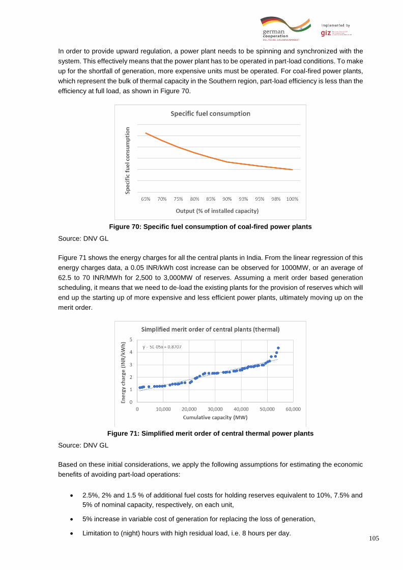
105

In order to provide upward regulation, a power plant needs to be spinning and synchronized with the

system. This effectively means that the power plant has to be operated in part-load conditions. To make

up for the shortfall of generation, more expensive units must be operated. For coal-fired power plants,

which represent the bulk of thermal capacity in the Southern region, part-load efficiency is less than the

efficiency at full load, as shown in Figure 70.

Figure 70: Specific fuel consumption of coal-fired power plants

Source: DNV GL

Figure 71 shows the energy charges for all the central plants in India. From the linear regression of this

energy charges data, a 0.05 INR/kWh cost increase can be observed for 1000MW, or an average of

62.5 to 70 INR/MWh for 2,500 to 3,000MW of reserves. Assuming a merit order based generation

scheduling, it means that we need to de-load the existing plants for the provision of reserves which will

end up the starting up of more expensive and less efficient power plants, ultimately moving up on the

merit order.

Figure 71: Simplified merit order of central thermal power plants

Source: DNV GL

Based on these initial considerations, we apply the following assumptions for estimating the economic

benefits of avoiding part-load operations:

• 2.5%, 2% and 1.5 % of additional fuel costs for holding reserves equivalent to 10%, 7.5% and

5% of nominal capacity, respectively, on each unit,

• 5% increase in variable cost of generation for replacing the loss of generation,

• Limitation to (night) hours with high residual load, i.e. 8 hours per day.

106

Based on these assumptions, we have calculated the economic benefits of avoiding part-load

operation, as shown in Table 27. Part-load losses are estimated in a range of INR 2.1 to 11.5 million

per year and the cost of additional generation is from 0.4 to 1.9 million INR per year which results in the

total avoided cost of 2.6 to 13.4 billion INR per year.

Table 27: Estimated economic benefits of avoiding part-load operation

Assumptions Unit Min Average Max

Reserve requirements MW 2,500 2,750 3,000

Reserves held on each unit % of Pnom 10.0% 7.5% 5.0%

Part load losses % of fuel costs 2.5% 2.0% 1.5%

Plants providing capacity MW 25,000 36,667 60,000

Energy charges INR/kWh 1.2 2.3 4.4

Estimated costs

Part load losses INR billion 2.1 5.0 11.5

Costs of additional generation (5% increase)

INR billion 0.4 0.9 1.9

Avoided costs INR billion 2.6 5.9 13.4

Source: DNV GL

The holding of downward reserves may result in increasing must run requirements during periods of

low load. However, the limited impact of regional dimensioning on volumes of downward regulation has

been observed from the analysis. Moreover, the effect will only become critical during hours of low

residual load on days with a large swing of residual load only which is unlikely to occur every day. Since

the downward regulation may also be achieved by temporary, the cost of increased holding of

downward reserves remains small compared to other effects described above and hence neglected

from our analysis.

In addition to the effects described above, more frequent and faster ramping of thermal power plants

causes additional wear and tear. But the literature suggests that the wear and tear costs are

substantially smaller than the costs of part-load operations, and hence neglected from our analysis.

The total benefits of reserve sharing are summarized in Table 28. Calculations show that the benefits

of reserve sharing are significant. Total benefits may range between INR 15 and 29 bn per year with a

mid-estimate of INR 20 bn per year. From the table below, it can be observed that the overall benefits

are dominated by capacity-related effects.

Table 28: Summary of avoided costs due to joint dimensioning

Avoided costs (INR bn/a) Min Average Max

Reserve Capacity 12.9 14.2 15.5

Part-load operations 2.6 5.9 13.4

Must-run caused by downward regulation Neglected / Limited

Additional wear and tear Neglected / Limited

Total 15.5 20.1 28.9

107

8.3.2 Joint procurement of reserves

Estimating the potential savings due to joint procurement of reserves is aggravated by several

challenges, especially the lack of truly commercial or market-based arrangements for reserve provision

in India, especially at the state level. Nevertheless, it seems reasonable to assume that joint

procurement offers substantial scope for potential savings considering the uneven distribution of flexible

capacities, local and reserve needs in the Southern region, see Figure 72. Furthermore, savings should

also result from different cost levels for reserves. For instance, whilst some states have access to

hydropower, others likely have to rely on thermal plants. Finally, the joint procurement of reserves also

increases the scope for competition.

Figure 72: Installed capacity vs. load and reserve requirements in the Southern region (MW)

Source: DNV GL analysis

The following assumptions have been made to calculate the economic benefits:

• As a proxy for improved efficiency of reserve activation, we assume fuel savings of 2.5%, 5%,

and 10%.

• As before, we focus on upward reserves during night hours since sufficient spare capacity is

available during day hours.

• Assuming that total reserve needs outside day hours (i.e. hours without PV) are in a range of

at least 2,000 MW and that 50% of total reserves may be traded between states, we assume

a potential of 1,000 MW.

Hydro

Hydro

Hydro

Hydro?

108

Furthermore, we differentiate between two alternative cases as follows:

• Case 1: Spare capacity is available from hydropower, which can be exported to other states

and replace reserve provision on thermal plants. When neglecting the opportunity costs of

holding reserves on unused hydropower plants, potential savings correspond to the variable

costs of thermal plants.

• Case 2: Reserves must be provided by thermal plants as hydropower plants will be operating

at high loading and the reserves need to be provided by thermal plants. In this case, we apply

the same assumptions as for the estimation of part-load losses above.

Table 29 provides an overview of the corresponding calculations and the resulting estimates. For case

1, we estimate the avoided cost due to joint procurement for Case-I has been calculated to be between

1 to 4.5 billion INR per year. Conversely, case II leads to potential savings of between 0.1 to 1.9 billion

INR. Assuming 50:50 split between both the above cases, total savings can be estimated to be in the

range of 0.5 to 3.2 billion INR per year.

Table 29: Estimated economic benefits due to the joint procurement of reserves

Reserve exchange – thermal only Min Average Max

Reserve requirements MW 1,000 1,000 1,000

Energy charges INR/kWh 1.17 2.33 4.36

Fuel savings % 2.5% 5.0% 10.0%

Fuel savings INR/kWh 0.03 0.12 0.44

Avoided costs INR billion 0.1 0.5 1.9

Reserve exchange - thermal to hydro

Reserve requirements MW 1,000 1,000 1,000

Avoided part load losses INR/kWh 1.05 4.82 15.39

Fuel savings % 2.5% 5.0% 10.0%

Fuel savings INR/kWh 0.03 0.24 1.54

Avoided costs INR billion 1.0 2.2 4.5

Source: DNV GL analysis

8.3.3 Imbalance netting

To estimate the impact of imbalance netting, we have simulated the (residual) system deviations to be

compensated by secondary and tertiary reserves for each individual state as well as at the regional

level. For each type of reserves, we have simulated stochastic generator outages as well as load, wind

and solar forecast errors for 10,000 ‘hours’ or time periods, using the same assumptions as applied for

the probabilistic analysis under Task 3 above. In this context, we have neglected any correlation of

spatial deviations between individual states, noting that these likely over-estimates potential savings, in

particular for tertiary control. Furthermore, a time horizon of 0.5 h has again been used for secondary

reserves, whereas tertiary reserves are represented by a time horizon of 2 hours. The individual results

have then been used to determine the imbalance of each state and of the central plants as well as the

net residual imbalance of the entire region (i.e. by ‘netting’ of by individual imbalances).

To analyse the impact of increasing penetration of variable RE, the analysis has been separately carried

out for the present situation (Status quo 2018) as well as for the 100S-60W scenario for the year 2022.

109

For each scenario, a separate set of simulations was performed for four different dispatch situations as

follows:

• At 12 h and 20 h, reflecting situations with and without PV resp. day and night hours,

• On the corresponding ‘Peak’ and ‘Low’ days, corresponding to situations with and without wind.

These four situations represent the key differences in generation dispatch and reserve requirements.

Moreover, an analysis of the 11 years of synthetic time series of residual load determined under Task 3

above has shown that all four combinations stand for a roughly similar share of different outcomes over

time. By considering the average results for all four situations, it is thus possible to adequately capture

different conditions throughout the year.

Figure 73 provides an overview of the average avoided activation of secondary and tertiary reserves

for the Southern region, expressed in percent of the sum of the individual deviations for all five states

and the central plants. This summary allows for the following observations:

• In line with experiences from Europe, imbalance netting allows for a significant reduction of

reserve activation. Based on the simulations performed, the volume of energy activated from

secondary and tertiary reserves may be reduced by some 40% and 50% for upward as well as

downward regulation.

• Relative savings are lesser for upward than for downward regulation since generator outages

in individual states are not correlated with each other.

• Potential savings decrease in the 100S-60W scenario, reflecting the assumption of a symmetric

distribution and the lack of any spatial correlation of positive and negative state-wise deviations

of wind and solar power 22 .

Although this is not shown in Figure 73, it is worth noting that absolute savings strongly increase from

2018 to 2022, especially during day hours (PV) and periods with wind (‘Low’ scenario). Again, this

clearly shows the impact of variable RE.

As mentioned, the results presented in Figure 73 do not account for any spatial correlation of forecast

errors (wind, solar, load), which may reasonably be expected in practice. To avoid unrealistic results,

we, therefore, apply a more conservative estimate of 30% potential savings for further analysis, noting

that this roughly corresponds to experiences from Europe as presented in section 8.2.3 above.

22 Except for the 20 h snapshot in the ‘Peak’ scenario, which is characterized by the absence of PV and minimal

generation from wind power.

110

In percent of situation without netting

Average values, based on 10,000 simulated values per combination

Figure 73: Avoided activation of secondary and tertiary reserves due to imbalance netting

Source: DNV GL analysis

Under the assumptions, the total annual volume of avoided balancing energy due to imbalance netting

increases from 1.7 TWh to nearly 2.9 TWh in 2022 (see Table 30), which is equivalent to 0.5% to 0.7%

of annual consumption in the southern region in the corresponding years. As Table 30, these savings

correspond to estimated annual savings of between INR 1.4bn in 2018 and INR 2bn in 2022. These

estimates are based on the following assumptions:

• In line with the current rules for the remuneration of energy delivered by RRAS (compare review

of the present situation under Task 1), the costs of upward regulation have been valued at

variable generation charges plus a mark-up of 0.5 INR/kWh.

• Similarly, the value of energy from downward regulation has been set equal to 75% of variable

generation charges.

• In line with the assumptions in section 8.3.1, variable generation charges are assumed to be in

a range of 1.5 – 3.5 INR/kWh, with a base estimate of 2.5 INR/kWh.

Subject to these assumptions, monetary savings of imbalance netting can be estimated to be in a range

of INR 1.0bn – 1.8bn /a in 2018, but INR 1.5bn – 2.5bn /a in 2022.

Table 30: Estimated economic benefits of imbalance netting

Source: DNV GL analysis

Hour of day

Time horizon (h) 0.5 2 0.5 2 0.5 2 0.5 2

Upwards 51% 46% 50% 42% 51% 50% 52% 48%

Downwards 53% 58% 58% 67% 51% 53% 54% 58%

Absolute sum 52% 51% 54% 51% 51% 51% 53% 52%

12 20 12 20

Peak lowScenario

Status quo 2018

Hour of day

Time horizon (h) 0.5 2 0.5 2 0.5 2 0.5 2

Upwards 47% 46% 51% 44% 47% 47% 51% 48%

Downwards 48% 49% 59% 65% 47% 47% 53% 56%

Absolute sum 47% 47% 55% 52% 47% 47% 52% 52%

12 20 12 20

Scenario100S-60W

Peak low

0.5 2 0.5 2 0.5 2 0.5 2

Upward 333 612 573 950 1.00 1.84 1.72 2.85

Downward 317 446 554 803 -0.59 -0.84 -1.04 -1.51

Total 650 1,058 1,126 1,753 0.41 1.00 0.68 1.34

Sum

2022 2018 2022

1,708 2,880 1.40 2.02

2018

Assuming 30% volume savings

Savings (GWh/a) Economic benefits (INR bn/a)

111

8.3.4 Joint activation of secondary and tertiary reserves (common merit order)

Similar to the joint procurement of reserves, the use of a common merit order for secondary and tertiary

reserves, respectively, may allow for cost savings due to more efficient use of available resources.

Whilst increasing competition may lead to further cost savings, this aspect is again neglected, due to

the current lack of explicit commercial arrangements at the state level.

In contrast to the previous analysis, we now consider the activated volume of balancing energy from

secondary and tertiary reserves. Since the use of a common merit order implicitly implies imbalance

netting, we furthermore again assume that 30% of activated reserves can be avoided. Under these

assumptions, the residual need for balancing energy amounts to about some 6 TWh in 2019 but 9.6

TWh in 2022; see Table 31.

For estimating the resulting economic benefits, we again assume that the joint procurement of balancing

energy may allow for about 5% savings in fuel costs (compare section 8.3.2). When again applying

RRAS pricing and energy charges of 1.5 – 3.5 INR/kWh, this corresponds to annual savings of less than

INR 0.5 billion per annum

Table 31: Estimated economic benefits of imbalance netting

Source: DNV GL analysis

8.3.5 Summary

Table 32 presents a summary of the estimated economic benefits as derived in the previous sections.

From this comparison, it is clearly visible that reserve sharing has by far the largest savings potential.

In fact, the corresponding savings are about an order of magnitude larger than those in any other area.

This highlights that irrespective of the underlying uncertainties, the joint dimensioning of reserves can

be expected to generate by far the largest savings and should thus be considered as a priority.

Secondly, we note that the potential benefits of imbalance netting and exchange of reserves are in a

similar range. It is thus difficult to establish any clear preference for either option. Any decision on the

possible introduction of either approach should thus also consider the associated costs and complexity

of implementation. In this context, we also note that imbalance netting basically requires changes to

real-time activation of secondary and/or tertiary reserves, whereas the joint procurement of reserves

depends on the existence and harmonisation of clear commercial, ideally market-based arrangements

for reserve procurement.

Finally, Table 32 also indicates that potential savings from joint activation of balancing energy appear

to be the smallest. Furthermore, they require clear and fully harmonised arrangements for the offering,

real-time activation, and settlement of secondary and/or tertiary reserves.

0.5 2 0.5 2 0.5 2 0.5 2

Upward 1,111 2,040 1,909 3,167 0.2 0.3 0.3 0.5

Downward -1,057 -1,487 -1,846 -2,678 -0.1 -0.1 -0.2 -0.3

Total 54 552 62 489 0.1 0.2 0.1 0.2

Sum

Absolute sum 5,694 9,600

Total savings (INR bn/a)

2018

607 551

2022

Assuming 30% volume savings

Total deviations (GWh/a)

2018 2022

0.2 0.3

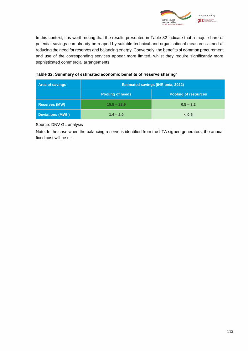
112

In this context, it is worth noting that the results presented in Table 32 indicate that a major share of

potential savings can already be reaped by suitable technical and organisational measures aimed at

reducing the need for reserves and balancing energy. Conversely, the benefits of common procurement

and use of the corresponding services appear more limited, whilst they require significantly more

sophisticated commercial arrangements.

Table 32: Summary of estimated economic benefits of ‘reserve sharing’

Area of savings Estimated savings (INR bn/a, 2022)

Pooling of needs Pooling of resources

Reserves (MW) 15.5 – 28.9 0.5 – 3.2

Deviations (MWh) 1.4 – 2.0 < 0.5

Source: DNV GL analysis

Note: In the case when the balancing reserve is identified from the LTA signed generators, the annual

fixed cost will be nill.

113

9 Conclusions and Recommendations

This document has investigated the impact of the expected growth of wind and solar power on the need

for secondary and tertiary control reserves in the Southern region. The application of a probabilistic

methodology for reserve dimensioning and consideration of several future scenarios allows for the

following observations and conclusions (compare Figure 74):

• The expected growth of VRE can be expected to lead to a (major) increase of current reserve

requirements, especially during day times.

• As forecast accuracy will become a major driver of future reserve needs, load despatch centres

at the national, regional and state levels will need to robust statistics on the variability and

forecast inaccuracy of wind and solar power, which requires access to reliable measurement

data from relevant plants.

• As reserve needs vary greatly for different conditions, a dynamic approach for reserve

dimensioning will become essential to help limiting reserve needs.

• As the sensitivity analysis under section 7.3 has shown, reserve volumes depend on the

desired safety margin. Given the hierarchical structure of system operation in India and the

principle of distributed action, Indian authorities should carefully consider the scope for sharing

risks between different regions as well as the interactions between different reserve products

and the intra-day wholesale market when deciding on the applicable safety margins.

• As illustrated by section 7.2, our calculations show clear benefits for joint dimensioning and

sharing of reserves at a regional level.

Most of these observations are either related to exogenous trends, data availability and/or the detailed

methodology for probabilistic reserve dimensioning. In contrast, the last observation depends on the

future organization and the distribution of rights and responsibilities for dimensioning, procurement and

activation of reserves between the state and regional (as well as national) level. This aspect will be

further considered under Task 4, where we will discuss and assess potential approaches for reserve

sharing and the corresponding economic benefits.

Figure 74: Key conclusions and recommendations

Source: DNV GL

Increasing penetration of VRE will likely lead to increasing reserve requirements

Forecast accuracy will become major driver of future reserve needs

Dynamic dimensioning helps to greatly reduce average reserve needs

Reserve volumes depend on desired safety margin, definition between different reserve products and interaction with (intraday) wholesale market

Calculations show clear benefits for joint reserve dimensioning and sharing

Supplying reserves exclusively by conventional plants likely to become very difficult and/or costly in the future

114

The latter will become even more important as the traditional supply of operating reserves by

conventional plants can be reasonably expected to become increasingly difficult and/or costly as the

penetration of VRE increases and the volume of synchronous conventional capacity decreases. In this

context, we finally note that the analysis in this document has been limited to the need for operating

reserves, whilst the potential supply and costs of these reserves have been beyond the scope of this

document.

115

10 References

[1] “http://www.cea.nic.in/reports/monthly/executivesummary/2018/exe_summary-03.pdf,” CEA 2018.

[2] “Report of the Expert Group on 175 GW RE by 2022 - NITI Aayog,” 2015.

[3] “http://www.cercind.gov.in/2016/regulation/9.pdf , last accessed on 5 March,2018”.

[4] “http://www.cercind.gov.in/2013/whatsnew/SP13.pdf,” CERC.

[5] “http://www.cercind.gov.in/2014/regulation/noti132.pdf, last accessed on 11 March 2019”.

[6] “http://www.cercind.gov.in/2018/regulation/dsm_fourth_amendment11-22-2018.pdf, last accessed on 11 March 2019”.

[7] “https://posoco.in/download/ancillary-services-report-for-january-19/?wpdmdl=21914, last accessed on 11 March 2019”.

[8] “Operationalization of Spinning Reserves,” POSOCO, July 2017.

[9] “Explanatory memorandum on introduction of ancillary services in India,” CERC, 2015.

[10] “Operationalization of Spinning Reserves,” July 2017.

[11] “https://www.gtg-india.com/automatic-generation-control-agc/ accessed on 15/04/2019”.

[12] “http://cercind.gov.in/2018/orders/08.pdf,” CERC Order.

[13] “http://cercind.gov.in/2018/orders/08.pdf,” CERC.

[14] “http://www.cercind.gov.in/2015/regulation/DAS.pdf, last accessed on 5 March,2019”.

[15] “http://www.iitk.ac.in/npsc/Papers/NPSC2016/1570291562.pdf, last accessed on 6 March,2019”.

[16] “http://www.cercind.gov.in/2016/regulation/14.pdf, last accessed on 6 March 2019”.

[17] “Introduction of Fast Response Ancillary Services 62nd FOR Meeting,” Forum of Regulators, April 2018.

[18] “http://www.cea.nic.in/reports/committee/nep/nep_jan_2018.pdf last accessed on 11 March 2019”.

[19] “http://www.cercind.gov.in/2015/orders/SO_11.pdf last accessed on 7 March 2019”.

[20] AEMO, “AEMO’s Frequency Control factsheet”.

[21] “GUIDE TO ANCILLARY SERVICES IN THE NATIONAL ELECTRICITY MARKET,” AEMO, 2015.

[22] “Power System Requirements,” AEMO, March 2018.

[23] AEMO, “https://www.aemo.com.au/Media-Centre/AEMO-market-notifications-explained”.

[24] “RULE DETERMINATION: National Electricity Amendment (Declaration of Lack of Reserve Conditions) Rule 2017,” Australian Energy Market Commission, December 2017.

[25] “Overview of new method for determining Lack of Reserve (LOR) levels – Feb 2018,” AEMO.

[26] “https://www.energy.gov/sites/prod/files/2015/12/f28/united-states-electricity-industry-primer.pdf last accessed on 14 March 2019”.

[27] “https://www.energy.gov/sites/prod/files/2017/02/f34/Appendix--Electricity%20System%20Overview.pdf last accessed on 14 March 2019”.

[28] “http://large.stanford.edu/courses/2010/ph240/sherer1/ last accessed on 14 March 2019”.

[29] “FERC 1995 last accessed on 13 March 2019”.

[30] “https://www.ferc.gov/legal/maj-ord-reg/land-docs/rm95-8-00w.txt last accessed on 13 March 2019”.

[31] “https://www.ferc.gov/about/ferc-does.asp?csrt=3447842511598895802 last accessed on 14 March 2019”.

[32] “https://www.energy.gov/sites/prod/files/2015/12/f28/united-states-electricity-industry-primer.pdf last accessed on 14 March 2019”.

[33] “https://www.ferc.gov/industries/electric/indus-act/rto.asp last accessed on 14 March 2019”.

[34] “https://www.ferc.gov/industries/electric/indus-act/rto.asp last accessed on 14 March 2019”.

[35] “https://www.nerc.com/Pages/default.aspx last accessed on 14 March 2019”.

[36] “https://www.ferc.gov/media/news-releases/2006/2006-3/07-20-06-E-5.asp last accessed on 16 March 2019”.

[37] “https://grid.lbl.gov/sites/all/files/report-lbnl-43986.pdf last accessed on 15 March 2019”.

[38] “https://www.nerc.com/files/glossary_of_terms.pdf last accessed on 19 March 2019”.

[39] “https://www.eia.gov/todayinenergy/detail.php?id=27152 last accessed on 23 March 2019”.

116

[40] “https://www.caiso.com/Documents/ReliabilityCoordinatorFAQ.pdf last accessed on 19 March 2019”.

[41] “https://www.nerc.com/pa/rrm/TLR/pages/reliability-coordinators.aspx last accessed on 23 March 2019”.

[42] “https://www.nerc.com/files/glossary_of_terms.pdf last accessed on 19 March 2019”.

[43] “http://www.caiso.com/about/Pages/default.aspx last accessed in 13 March 2019”.

[44] “https://afdc.energy.gov/files/pdfs/2527.pdf last accessed on 13 March 2019”.

[45] “http://www.caiso.com/market/Pages/MarketProcesses.aspx last accessed on 13 March 2019”.

[46] “http://www.caiso.com/about/Pages/OurBusiness/The-ISO-grid.aspx last accessed on 23 March 2019”.

[47] “https://www.caiso.com/Documents/AncillaryServicesOverview.pdf last accessed on 13 March 2019”.

[48] “http://oasis.caiso.com/mrioasis/logon.do last accessed on 14 March 2019”.

[49] “http://www.caiso.com/market/Pages/MarketProcesses.aspx last accessed on 15 March 2019”.

[50] “http://www.caiso.com/participate/Pages/MarketProducts/AncillaryServices/Default.aspx last accessed on 25 March 2019.”.

[51] “https://www.nerc.com/pa/Stand/Reliability%20Standards/BAL-001-2.pdf last accessed on 16 March 2019”.

[52] “http://www.caiso.com/Documents/Section8_AncillaryServices_Jul1_2013.pdf last accessed on 19 March 2019”.

[53] “http://oasis.caiso.com/mrioasis/logon.do last accessed on 19 March 2019”.

[54] “https://www.nerc.com/docs/pc/ivgtf/NERC_ancillary_services%20ERCOT%20IESO%20NYISO%20MISO%20PJM%20SPP%20WECC%2012%2014.pdf last accessed on 18 March 2019”.

[55] “https://www.nerc.com/docs/pc/ivgtf/NERC_ancillary_services%20ERCOT%20IESO%20NYISO%20MISO%20PJM%20SPP%20WECC%2012%2014.pdf last accessed on 18 March 2019”.

[56] “entsoe. Supporting Document for the Network Code on Load-Frequency Control and Reserves. Brussels. 28.06.2013”.

[57] “dena. dena Ancillary Services Study 2030. Security and reliability of a power supply with a high percentage of renewable energy. Final report. Final report. Berlin, 2014”.

[58] “Gürses, G., Garrison, J., Madlener, R. and T. Demiray. Economic and Operational Assessment of Reserve Methods and Metrics for Electric Grids with High Shares of Renewables. FCN Working Paper No. 22/2016. December 2016, Revised May 2017”.

[59] M. Lange, “Präzise Wind- und Solarleistungsvorhersagen - Unverzichtbar für die Energiewende Unverzichtbar für die Energiewende.,” Aachen, 2016.

[60] NREL, “Greening the Grid : Pathways to integrate 175 GW Renewable energy into India's Electric Grid, Vol.1 National Study”.

[61] NREL, “Greening the Grid : Pathways to integrate 175 GW Renewable energy into India's Electric Grid, Vol.2 Regional Study”.

[62] CEA, “National electricity plan - Generation 2017-22”.

[63] C. E. A. (CEA), “Review of performance of hydro power stations 2017-18”.

[64] CEA, “ANNUAL PERFORMANCE REVIEW OF THERMAL POWER STATIONS FOR 2014-15’ (CEA)”.

[65] “http://www.cercind.gov.in/2010/ORDER/February2010/IEGC_Review_Proposal.pdf, last accessed on 5 March,2019”.

[66] “http://erpc.gov.in/wp-content/uploads/2018/03/RGMO-presentation-37th-TCC.pdf, last accessed on 11 March 2019”.

[67] “http://www.cercind.gov.in/2017/orders/79_rc.pdf, last accessed on 11 March 2019”.

[68] “http://www.cercind.gov.in/2015/draft_reg/Ancillary_Services.pdf last accessed on 11 March 2019”.

[69] “http://www.cercind.gov.in/2016/regulation/9.pdf , Last accessed on 7 March 2019”.

[70] DENA, “Ancillary services study 2030.Security and reliability of a power supply with a high percentage of renewable energy,” 2014.

117

11 Appendices

Appendix A. Overview of results for 70S-45W

70S-45W Peak

Scenario Lead time Forecast quality Outage rates Risk margin Adapt. forecast

70S-45W Peak 0.5h 100% 250% 0.1% Yes

Figure 75: Secondary and tertiary reserves in 70S-45W Peak Scenario

118

70S-45W Low

Scenario Lead time Forecast quality Outage rates Risk margin Adapt. forecast

70S-45W Low 0.5h 100% 250% 0.1% Yes

Figure 76: Secondary and tertiary reserves in 70S-45W Low Scenario

119

Appendix B. Overview on results for 60S-100W

60S-100W Peak

Scenario Lead time Forecast quality Outage rates Risk margin Adapt. forecast

60S-100W Low 0.5h 100% 250% 0.1% Yes

Figure 77: Secondary and tertiary reserves in 60S-100W Peak Scenario

120

60S-100W Low

Scenario Lead time Forecast quality Outage rates Risk margin Adapt. forecast

60S-100W Low 0.5h 100% 250% 0.1% Yes

Figure 78: Secondary and tertiary reserves in 60S-100W Low Scenario

121

Appendix C. Overview on results with Confidence Level of 99.50% and Outage rate of 150%

Status Quo 2018 Peak Status Quo 2018 Low

Scenario Lead time Forecast quality Outage rates Risk margin Adapt. forecast

Status quo 2018 2h 100% 150% 0.5% Yes

Figure 79: Sum of secondary and tertiary reserve vs. regionally required reserves, status quo 2018 scenario

122

150S-100W Peak 150S-100W Low

Scenario Lead time Forecast quality Outage rates Risk margin Adapt. forecast

150S-100W 2h 100% 150% 0.5% Yes

Figure 80: Sum of secondary and tertiary reserve vs. regionally required reserves, 150S-100W scenario

Imprint The findings and conclusions expressed in this document do not necessarily represent the views of the

GIZ or BMZ. The information provided is without warranty of any kind.

Published by

Deutsche Gesellschaft für

Internationale Zusammenarbeit (GIZ) GmbH

Indo – German Energy Programme – Green Energy Corridors

Registered offices: Bonn and Eschborn, Germany

B-5/2, Safdarjung Enclave

New Delhi 110 029 India

T: +91 11 49495353

E: info@giz.de

I: www.giz.de

Office Responsible for Project Implementation

Markus Wypior, GIZ

Authors

Christian Hewicker, DNV GL

Alok Kumar, DNV GL

Alok Kumar Mishra, DNV GL

Musab Arappil, DNV GL

Editor

Sunil Sharma, GIZ

This project/programme’ assisted by the German Government, is being carried out by Garrad Hassan

India Private Limited (DNV GL) on behalf of the Deutsche Gesellschaft für Internationale

Zusammenarbeit (GIZ) GmbH.

Consultant