Dimensionality Reduction John Freddy Duitama

U. de A. - UN.

Index

•  Motivation •  Eigenvalues and Eigenvectors •  Principal-Component Analysis •  Singular-Value Decomposition

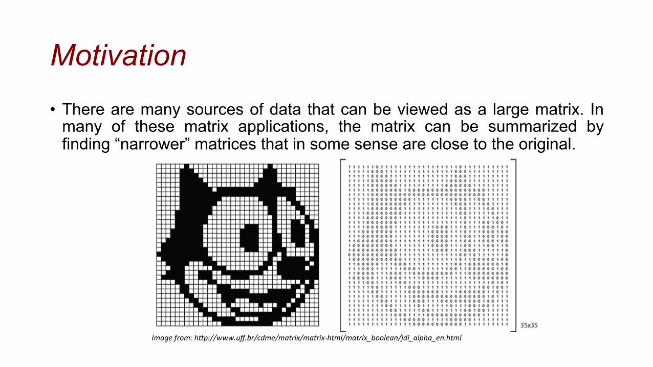
Motivation •  There are many sources of data that can be viewed as a large matrix. In

many of these matrix applications, the matrix can be summarized by finding “narrower” matrices that in some sense are close to the original.

Image  from:  h,p://www.uff.br/cdme/matrix/matrix-­‐html/matrix_boolean/jdi_alpha_en.html  

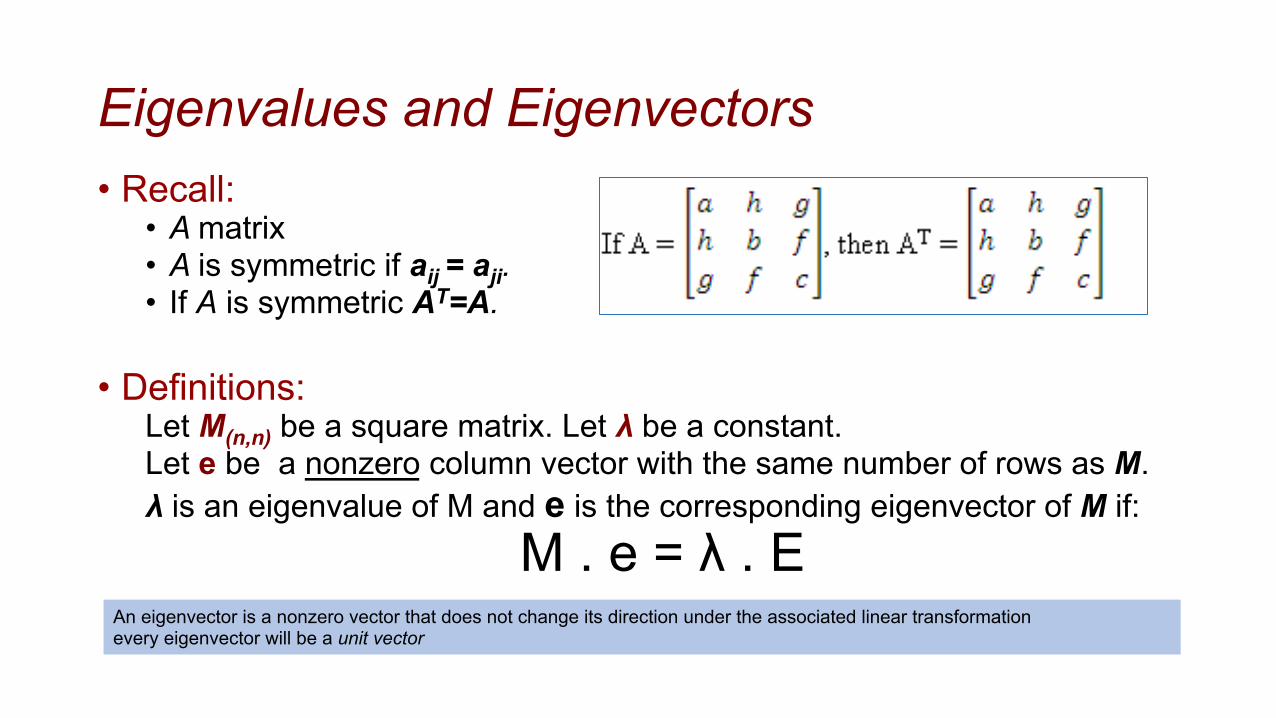
Eigenvalues and Eigenvectors • Recall:

•  A matrix •  A is symmetric if aij = aji. •  If A is symmetric AT=A.

• Definitions: Let M(n,n) be a square matrix. Let λ be a constant. Let e be a nonzero column vector with the same number of rows as M. λ is an eigenvalue of M and e is the corresponding eigenvector of M if:

M . e = λ . E

An eigenvector is a nonzero vector that does not change its direction under the associated linear transformation every eigenvector will be a unit vector

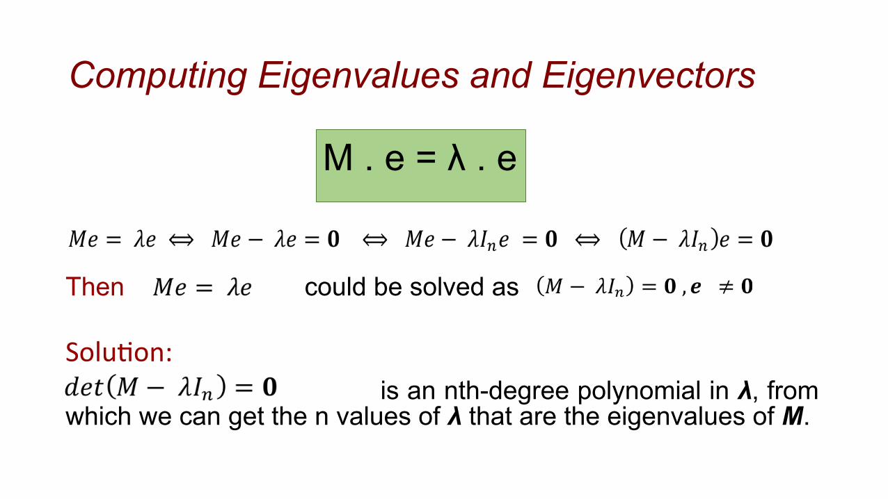
Computing Eigenvalues and Eigenvectors

Then could be solved as

 Solu&on:                                                                 is an nth-degree polynomial in λ, from which we can get the n values of λ that are the eigenvalues of M.

M . e = λ . e  

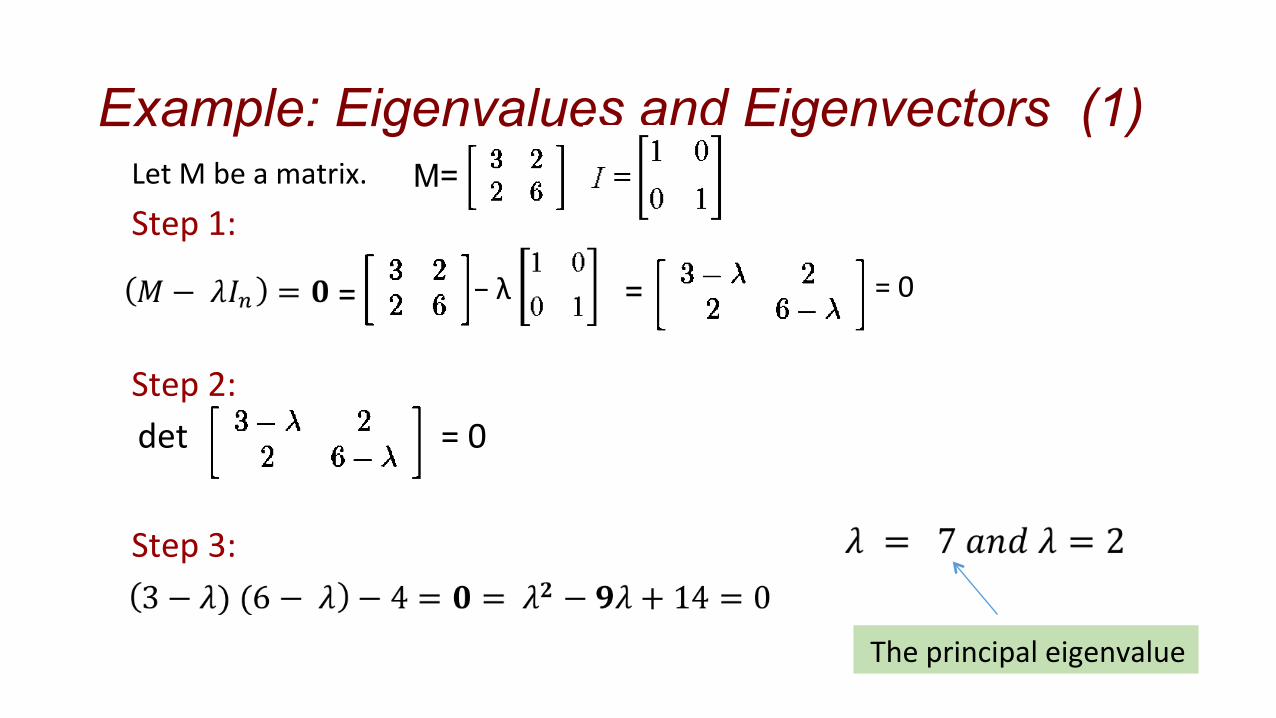
Let  M  be  a  matrix.                                                                            Step  1:      Step  2:      Step  3:                                      

Example: Eigenvalues and Eigenvectors (1) M=

−  λ =  0 =

det                                                            =  0        

     =    

 The  principal  eigenvalue  

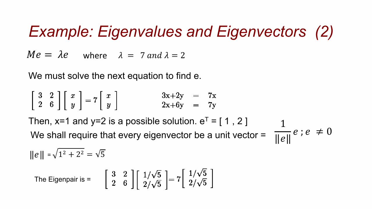
Example: Eigenvalues and Eigenvectors (2)

We must solve the next equation to find e.

Then, x=1 and y=2 is a possible solution. eT = [ 1 , 2 ]  We shall require that every eigenvector be a unit vector =

where    

=  

The Eigenpair is =  

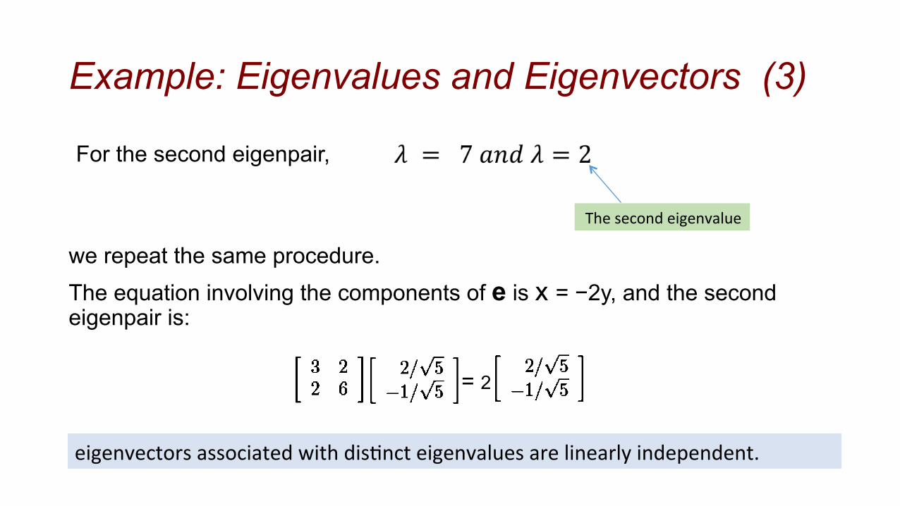
Example: Eigenvalues and Eigenvectors (3)

For the second eigenpair, we repeat the same procedure. The equation involving the components of e is x = −2y, and the second eigenpair is:

= 2

 The  second  eigenvalue  

eigenvectors  associated  with  dis&nct  eigenvalues  are  linearly  independent.  

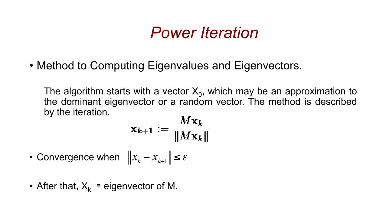
Power Iteration

• Method to Computing Eigenvalues and Eigenvectors.

The algorithm starts with a vector X0, which may be an approximation to the dominant eigenvector or a random vector. The method is described by the iteration.

•  Convergence when

•  After that, Xk ≅ eigenvector of M.

xk − xk+1 ≤ ε

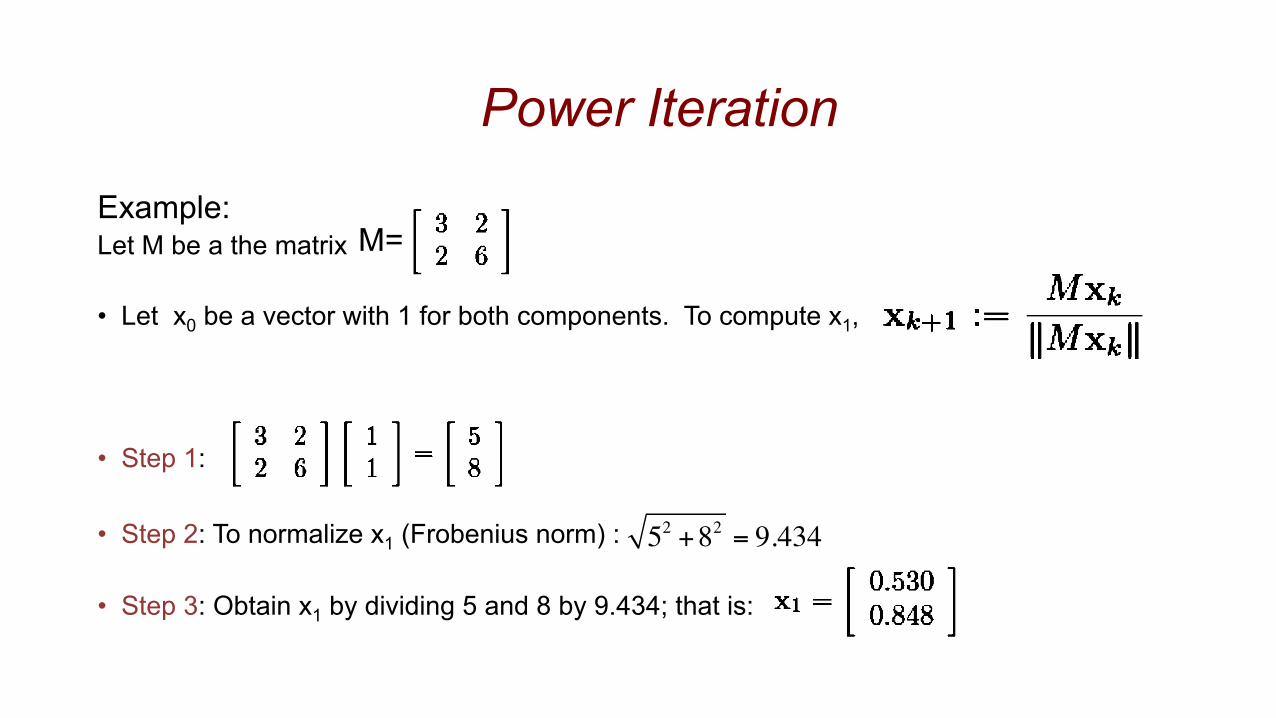
Example: Let M be a the matrix •  Let x0 be a vector with 1 for both components. To compute x1,

•  Step 1: : •  Step 2: To normalize x1 (Frobenius norm) :

•  Step 3: Obtain x1 by dividing 5 and 8 by 9.434; that is:

Power Iteration

M=

52 +82 = 9.434

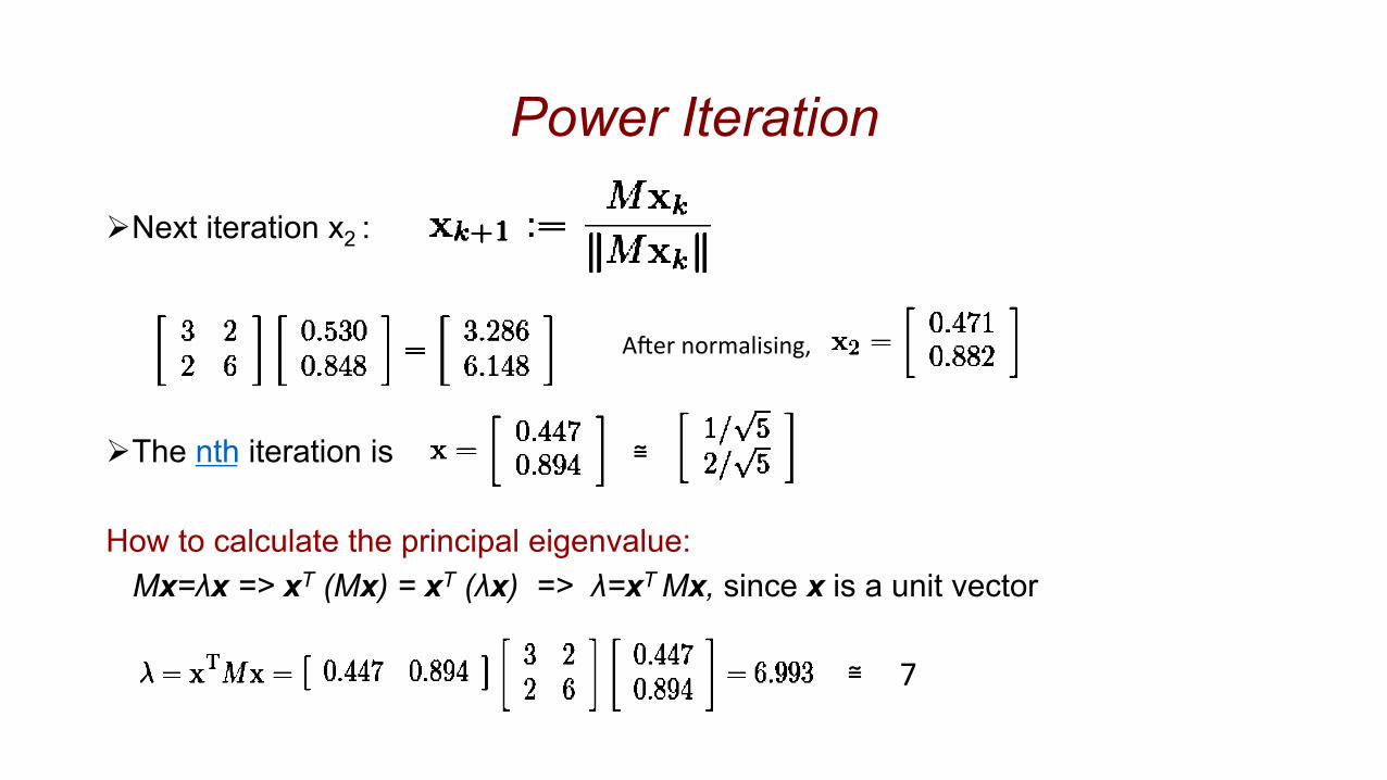
Ø Next iteration x2 :

Ø The nth iteration is

How to calculate the principal eigenvalue: Mx=λx => xT (Mx) = xT (λx) => λ=xT Mx, since x is a unit vector

Power Iteration

≅   7  

AGer  normalising,  

≅  

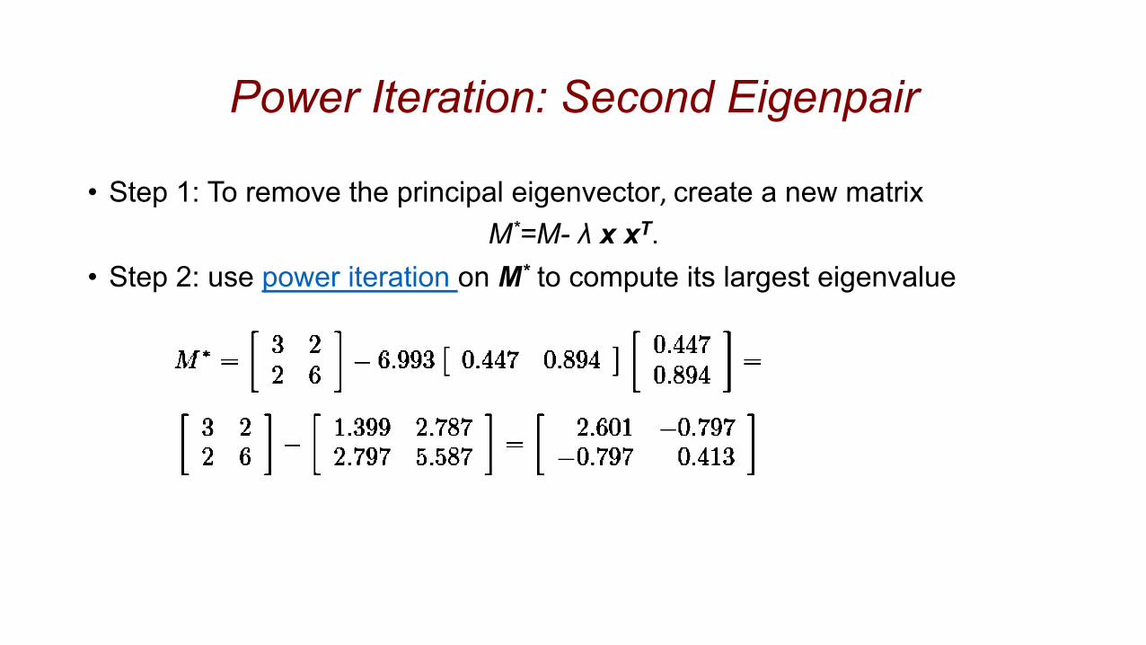
•  Step 1: To remove the principal eigenvector,  create a new matrix M*=M- λ x xT.

•  Step 2: use power iteration on M* to compute its largest eigenvalue

Power Iteration: Second Eigenpair

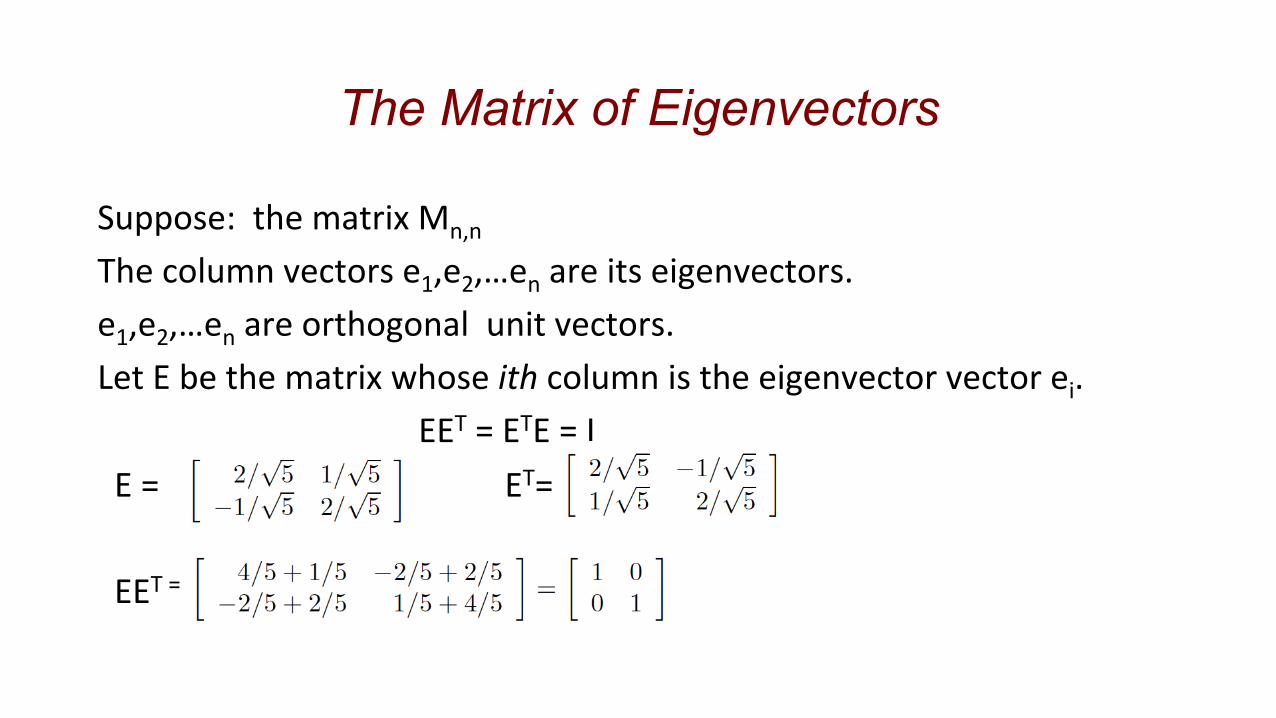
Suppose:    the  matrix  Mn,n  The  column  vectors  e1,e2,…en  are  its  eigenvectors.  e1,e2,…en  are  orthogonal    unit  vectors.  Let  E  be  the  matrix  whose  ith  column  is  the  eigenvector  vector  ei.                    EET  =  ETE  =  I          E  =                                                                                  ET=        EET  =    

The Matrix of Eigenvectors

Principal-Component Analysis (PCA)

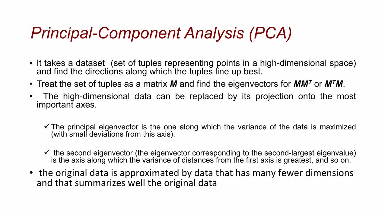
•  It takes a dataset (set of tuples representing points in a high-dimensional space) and find the directions along which the tuples line up best.

•  Treat the set of tuples as a matrix M and find the eigenvectors for MMT or MTM. •  The high-dimensional data can be replaced by its projection onto the most

important axes.

ü The principal eigenvector is the one along which the variance of the data is maximized (with small deviations from this axis).

ü  the second eigenvector (the eigenvector corresponding to the second-largest eigenvalue) is the axis along which the variance of distances from the first axis is greatest, and so on.

•   the  original  data  is  approximated  by  data  that  has  many  fewer  dimensions  and  that  summarizes  well  the  original  data

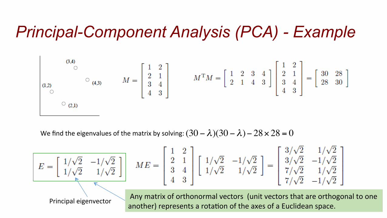
Principal-Component Analysis (PCA) - Example

We  find  the  eigenvalues  of  the  matrix  by  solving:    (30−λ)(30−λ)− 28×28 = 0

Principal  eigenvector    Any  matrix  of  orthonormal  vectors    (unit  vectors  that  are  orthogonal  to  one  another)  represents  a  rota&on  of  the  axes  of  a  Euclidean  space.  

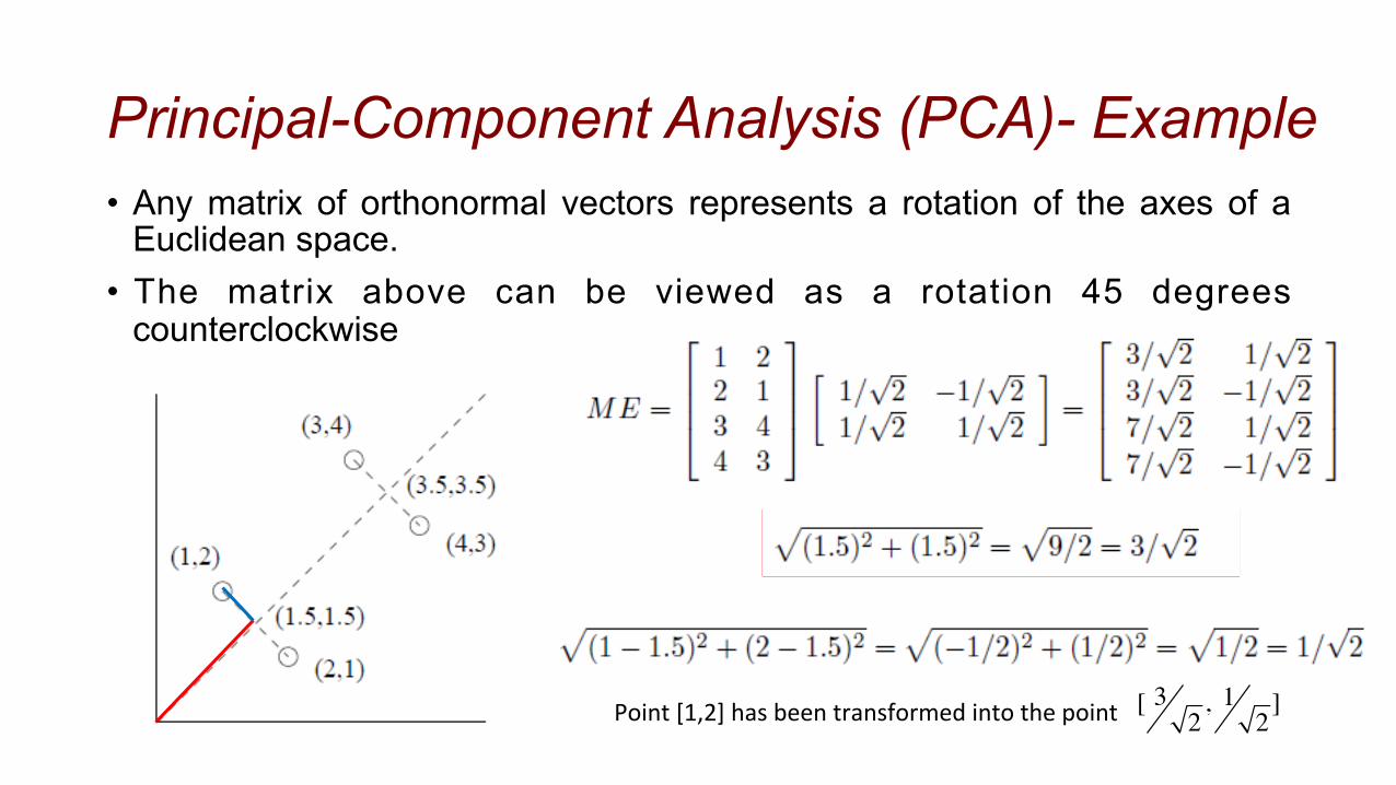
Principal-Component Analysis (PCA)- Example •  Any matrix of orthonormal vectors represents a rotation of the axes of a

Euclidean space. •  The matrix above can be viewed as a rotation 45 degrees

counterclockwise

Point  [1,2]  has  been  transformed  into  the  point            [ 3 2, 1

2]

Principal-Component Analysis (PCA)-Example

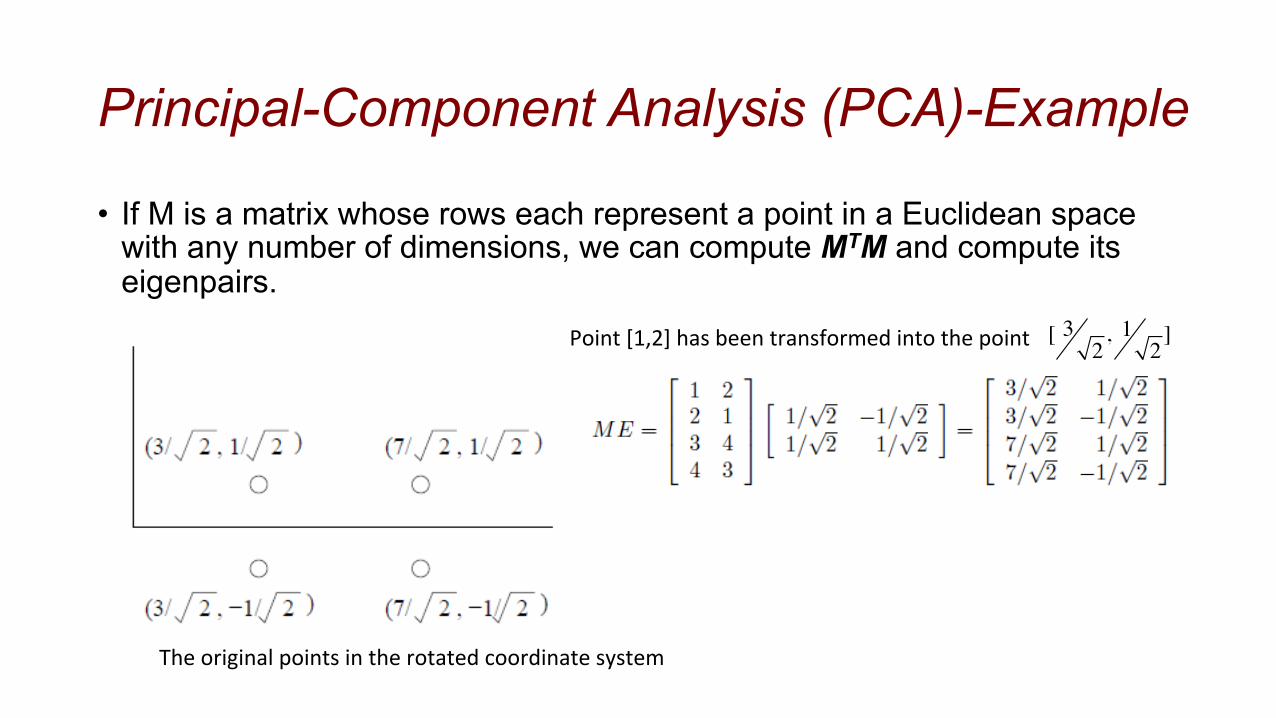
•  If M is a matrix whose rows each represent a point in a Euclidean space with any number of dimensions, we can compute MTM and compute its eigenpairs.

 The  original  points  in  the  rotated  coordinate  system  

Point  [1,2]  has  been  transformed  into  the  point            [ 3 2, 1

2]

Singular Value Decomposition

SVD allows an exact representation of any matrix, and also to eliminate the less important parts to produce an approximate representation with any desired number of dimensions. it is a method for transforming correlated variables into a set of uncorrelated ones that better expose the relationships among the original data items. A method for identifying and ordering the dimensions along which data points exhibit the most variation.

Singular Value Decomposition

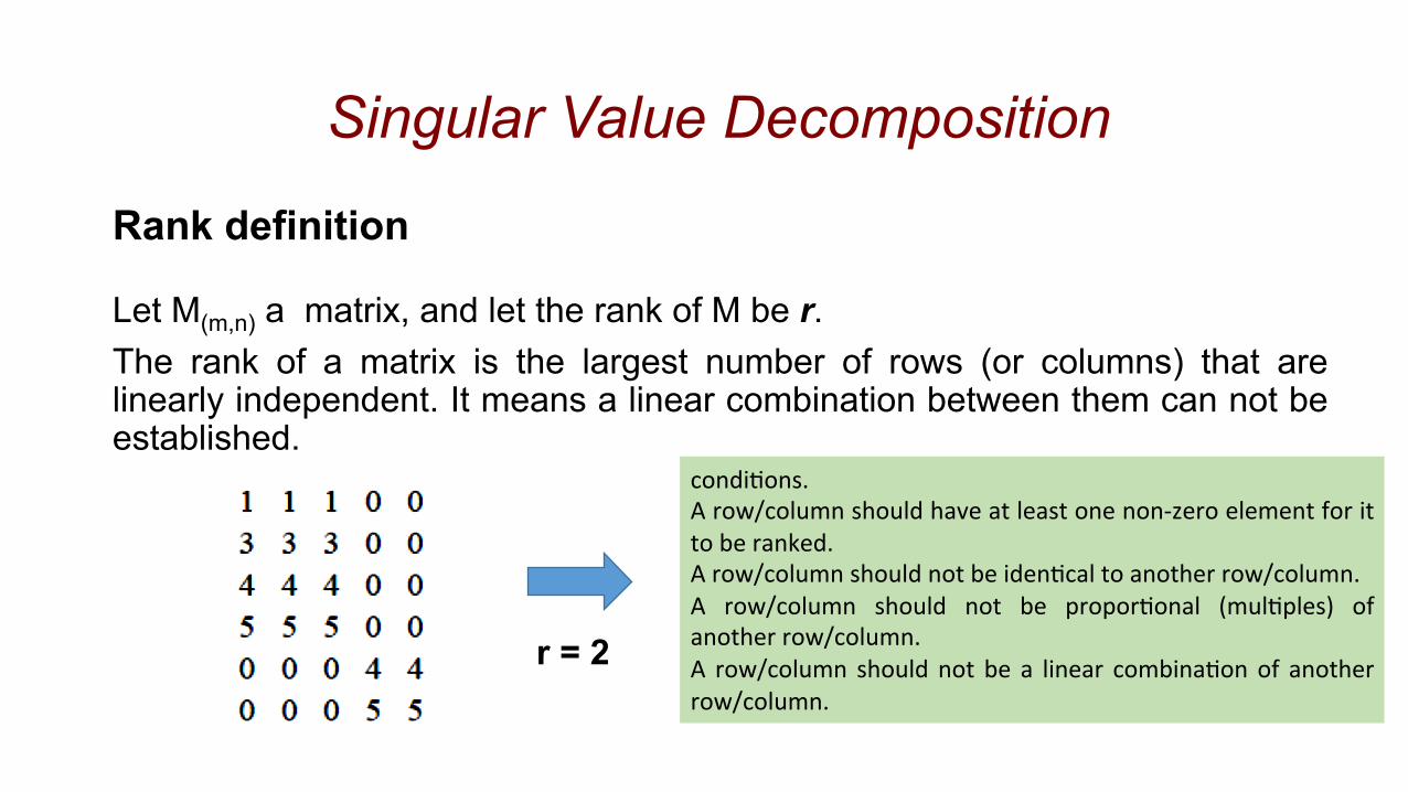
Let M(m,n) a matrix, and let the rank of M be r. The rank of a matrix is the largest number of rows (or columns) that are linearly independent. It means a linear combination between them can not be established.

Rank definition

r = 2

condi&ons.    A  row/column  should  have  at  least  one  non-­‐zero  element  for  it  to  be  ranked.    A  row/column  should  not  be  iden&cal  to  another  row/column.    A   row/column   should   not   be   propor&onal   (mul&ples)   of  another  row/column.    A   row/column   should  not   be   a   linear   combina&on  of   another  row/column.  

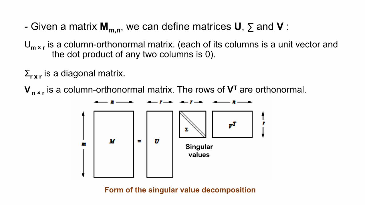
- Given a matrix Mm,n, we can define matrices U, ∑ and V : Um × r is a column-orthonormal matrix. (each of its columns is a unit vector and

the dot product of any two columns is 0). Σr x r is a diagonal matrix. V n × r is a column-orthonormal matrix. The rows of VT are orthonormal.

Form of the singular value decomposition

Singular values  

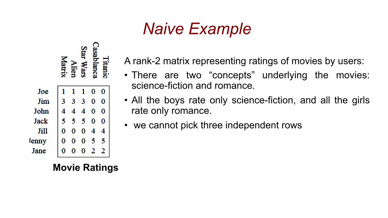
Movie Ratings

A rank-2 matrix representing ratings of movies by users: •  There are two “concepts” underlying the movies:

science-fiction and romance. •  All the boys rate only science-fiction, and all the girls

rate only romance. •   we cannot pick three independent rows

Naive Example

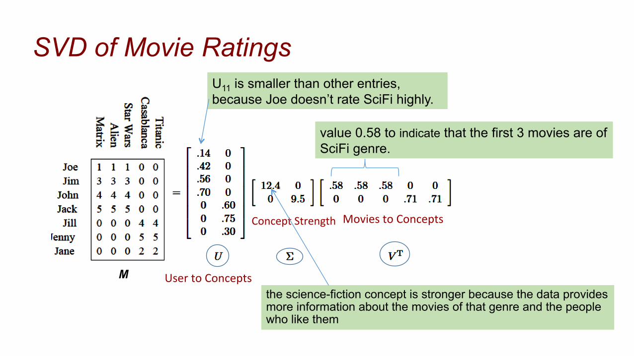
the science-fiction concept is stronger because the data provides more information about the movies of that genre and the people who like them

SVD of Movie Ratings

Concept  Strength  

User  to  Concepts  

Movies  to  Concepts    

M

U11 is smaller than other entries, because Joe doesn’t rate SciFi highly.

value 0.58 to indicate that the first 3 movies are of SciFi genre.

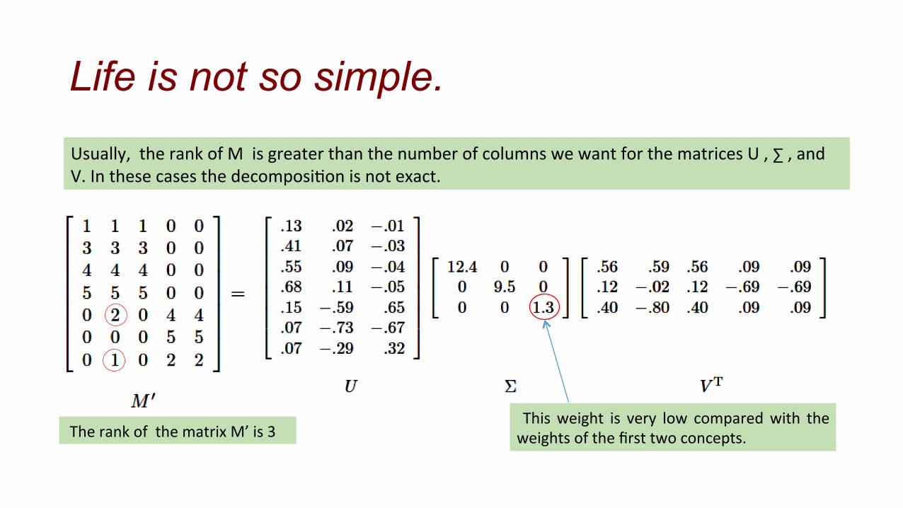
Life is not so simple.

Usually,    the  rank  of  M    is  greater  than  the  number  of  columns  we  want  for  the  matrices  U  ,  ∑  ,  and  V.  In  these  cases  the  decomposi&on  is  not  exact.

 The  rank  of    the  matrix  M’  is  3     This  weight   is   very   low   compared  with   the  weights  of  the  first  two  concepts.  

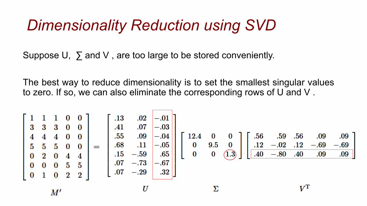
Dimensionality Reduction using SVD

Suppose U, ∑ and V , are too large to be stored conveniently. The best way to reduce dimensionality is to set the smallest singular values to zero. If so, we can also eliminate the corresponding rows of U and V .

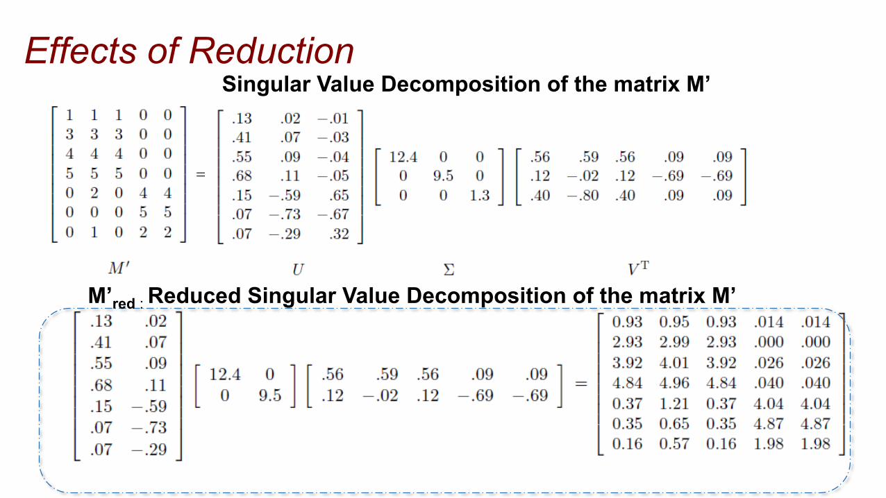
Singular Value Decomposition of the matrix M’ Effects of Reduction

M’red : Reduced Singular Value Decomposition of the matrix M’

Source  :  h\p://fourier.eng.hmc.edu/e161/lectures/svdcompression.html  

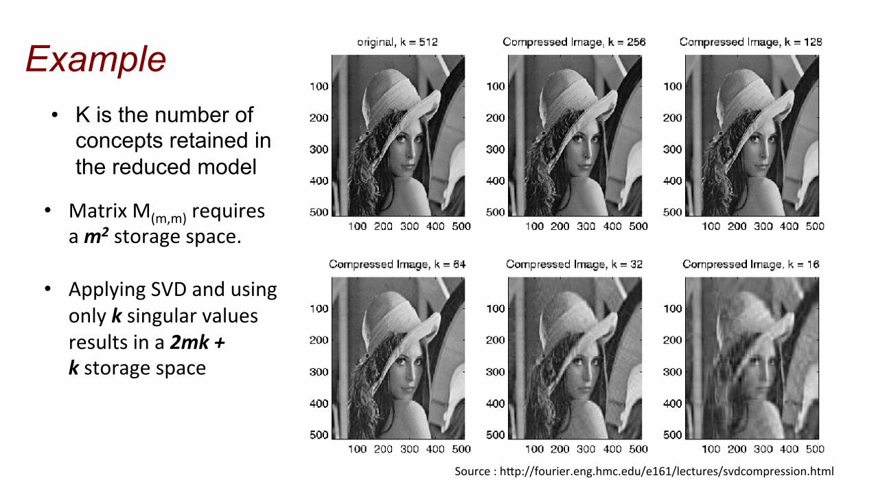
Example •  K is the number of

concepts retained in the reduced model

•  Matrix  M(m,m)  requires  a  m2  storage  space.    

•  Applying  SVD  and  using  only  k  singular  values  results  in  a  2mk  +  k  storage  space  

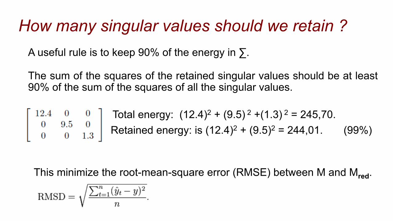
A useful rule is to keep 90% of the energy in ∑.

The sum of the squares of the retained singular values should be at least 90% of the sum of the squares of all the singular values.

Total energy: (12.4)2 + (9.5) 2 +(1.3) 2 = 245,70. Retained energy: is (12.4)2 + (9.5)2 = 244,01. (99%)

This minimize the root-mean-square error (RMSE) between M and Mred.

How many singular values should we retain ?

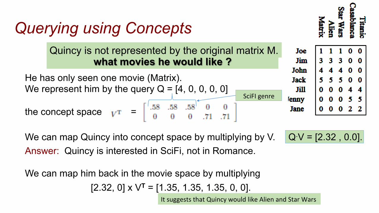
what movies he would like ?

Querying using Concepts

We can map Quincy into concept space by multiplying by V. Q.V = [2.32 , 0.0]. Answer: Quincy is interested in SciFi, not in Romance.

We can map him back in the movie space by multiplying [2.32, 0] x VT = [1.35, 1.35, 1.35, 0, 0].

Quincy is not represented by the original matrix M.

He has only seen one movie (Matrix). We represent him by the query Q = [4, 0, 0, 0, 0] the concept space =

SciFI  genre  

It  suggests  that  Quincy  would  like  Alien  and  Star  Wars  

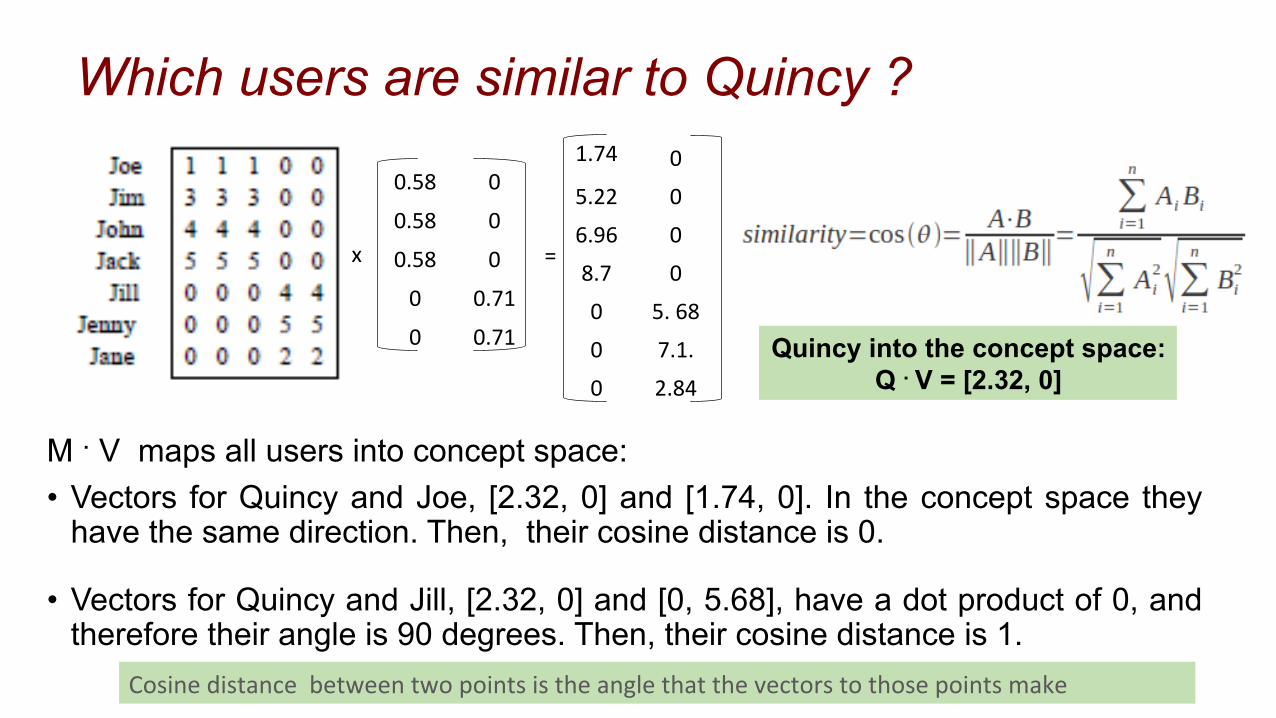
M . V maps all users into concept space: •  Vectors for Quincy and Joe, [2.32, 0] and [1.74, 0]. In the concept space they

have the same direction. Then, their cosine distance is 0.

•  Vectors for Quincy and Jill, [2.32, 0] and [0, 5.68], have a dot product of 0, and therefore their angle is 90 degrees. Then, their cosine distance is 1.

Which users are similar to Quincy ?

0.58   0  

0.58   0  

0.58   0  

0   0.71  

0   0.71  

1.74   0  

5.22   0  

6.96   0  

8.7   0  

0   5.  68  

0   7.1.  

0   2.84  

Quincy into the concept space: Q . V = [2.32, 0]  

x   =  

Cosine  distance    between  two  points  is  the  angle  that  the  vectors  to  those  points  make  

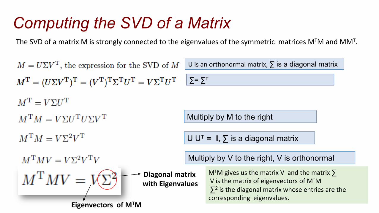
∑= ∑T

Computing the SVD of a Matrix

Multiply by M to the right

The  SVD  of  a  matrix  M  is  strongly  connected  to  the  eigenvalues  of  the  symmetric    matrices  MTM  and  MMT.  

Multiply by V to the right, V is orthonormal

Diagonal  matrix    with  Eigenvalues  

Eigenvectors    of  MTM  

U  is  an  orthonormal  matrix,  ∑ is a diagonal matrix    

U UT = I, ∑ is a diagonal matrix

MTM  gives  us  the  matrix  V    and  the  matrix  ∑  V  is  the  matrix  of  eigenvectors  of  MTM      ∑2  is  the  diagonal  matrix  whose  entries  are  the  corresponding    eigenvalues.      

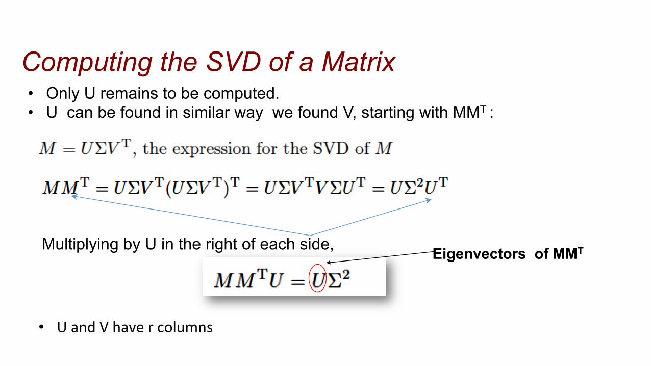
•  Only U remains to be computed. •  U can be found in similar way we found V, starting with MMT :

Multiplying by U in the right of each side, Eigenvectors of MMT

Computing the SVD of a Matrix

•  U  and  V  have  r  columns    

CUR decomposition

What happens when matrix M is sparse ? Most entries are 0

In this case, SVD is not optimal. There is a variant called CUR – decomposition.  

References

• Rajamaran  A.,  Leskovec  Jure  and  Ullman  J.D  (2014).  Mining  of  Massive  Datasets.  Cambridge  University  Press,  UK.  

• Baker,  Kirk    (2013).  Singular  Value  Decomposi&on  Tutorial.  DraG.    • Chame,  James  (2000).  Image  Compression  with  SVD.  [Online]  h\p://fourier.eng.hmc.edu/e161/lectures/svdcompression.html