Dimensionality Reduction in the Analysis of Human Genetics

Petros Drineas

Purdue UniversityDepartment of Computer Science

drineas

Dimensionality Reduction in the Analysis of Human Genetics Data

Petros Drineas

Purdue UniversityDepartment of Computer Science

drineas

Dimensionality Reduction in the Analysis of Human Genetics Data

PCA

Genotype

The average genome (~2x3 billion base pairs) contains:– 4-5 million single nucleotide variations, compared to the

reference sequence (Single Nucleotide Polymorphisms – SNPs)– ~0.5 million small insertions or deletions ‘indels’ (1-100bp)– ~5,000 larger insertions or deletions (>100bp)

We are quite similar, but we are different…

Variation across all (~23,000) genes - the ‘exome’~18,000 variants~8-9,000 functional variants~95% of variants are common~500-1000 genes with new mutations~100-200 knock-out mutations

Genetic variation is shaped by evolutionary forces• Mutation• Genetic drift• Population structure (inbreeding, mating patterns)• Gene flow and admixture• Natural selection

Early Homo sapiens sapiensin Africa

150,000 to 100,000 BP

Kidd Lab, Yale University, http://info.med.yale.edu/genetics/kkidd/point.html

~100,000 BP

Homo sapiens sapiensColonizing south west Asia

http://info.med.yale.edu/genetics/kkidd/point.html

Homo sapiens sapiens

~40,000 BP

http://info.med.yale.edu/genetics/kkidd/point.html

Tracking human migrations (out of Africa hypothesis)

Fact:

Linear Dimensionality Reduction techniques (such as Principal Components Analysis – PCA) separate different populations and result in plots that correlate well with geography or geo-demographics.

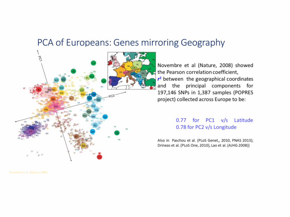
PCA for human genetic data analysis

𝑟𝑟2 = 0.77 for PC1 vs Latitude𝑟𝑟2 = 0.78 for PC2 vs Longitude

Novembre et al. (Nature 2008)

The success of PCA in (human) genetics is remarkable!

PCA has been around for over a century (Pearson 1901, Hotelling 1933).

PCA in human genetics goes back to (at least) Menozzi, Piazza, & Cavalli-Sforza (Science 1978).

Algorithms for PCA (meaning algorithms for SVD and eigendecompositions) have been a topic of intense research in numerical linear algebra and applied math for 70+ years.


The success of PCA in (human) genetics is remarkable!

PCA has been around for over a century (Pearson 1901, Hotelling 1933).

PCA in human genetics goes back to (at least) Menozzi, Piazza, & Cavalli-Sforza (Science 1978).

Algorithms for PCA (meaning algorithms for SVD and eigendecompositions) have been a topic of intense research in numerical linear algebra and applied math for 70+ years.

PCA has been very (?) successful in many domains:

Imaging: remember Eigenfaces? Document-term data: remember Latent Semantic Indexing (LSI)? Web search: remember HIITS and pagerank?

BUT the aforementioned domains have concluded that other (typically very non-linear) dimensionality reduction techniques are better in extracting structure in their respective modern datasets!


Fact:

Linear Dimensionality Reduction techniques (such as Principal Components Analysis – PCA) separate different populations and result in plots that correlate well with geography or geo-demographics.

Leverage this observation:

While we invariably use many other statistical techniques and software tools to analyze human genetic data, PCA plots are always the starting point and they often “set the tone” for other analyses.


Population genetics & histories of human populations

Mapping causative genes for common complex disordersCorrecting stratification in Genome-Wide Association Studies (GWAS)

Conservation studies

Forensics

Genealogy

Why do we care about and population structure?

Overview

• Scaling PCA to millions of samples/markers

• Selecting Ancestry Informative Markers (AIMs)

• PCA and Geodemographics

Mathematical apparatus:

• Subspace iteration vs. Krylov subspace methods to approximate principal components

• From the Singular Value Decomposition (SVD) to the CX decomposition, the Column Subset Selection Problem (CSSP), and beyond

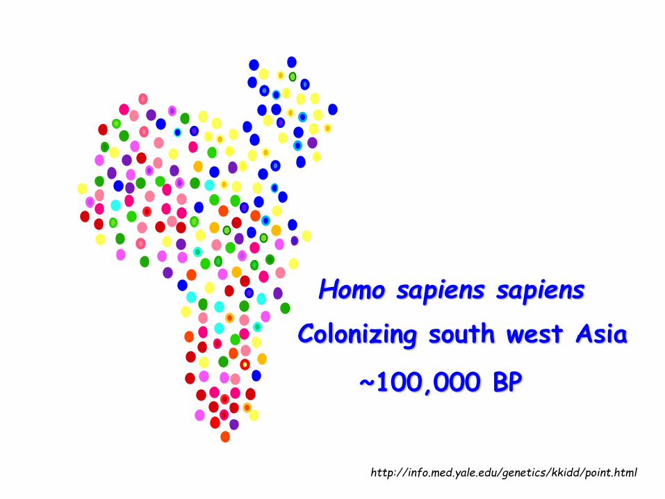
Single Nucleotide Polymorphisms (SNPs)

Single Nucleotide Polymorphisms: the most common type of genetic variation in the genome across different individuals.

They are known locations at the human genome where two alternate nucleotide bases (alleles) are observed (out of A, C, G, T).

SNPs

indi

vidu

als

… AG CT GT GG CT CC CC CC CC AG AG AG AG AG AA CT AA GG GG CC GG AG CG AC CC AA CC AA GG TT AG CT CG CG CG AT CT CT AG CT AG GG GT GA AG …… GG TT TT GG TT CC CC CC CC GG AA AG AG AG AA CT AA GG GG CC GG AA GG AA CC AA CC AA GG TT AA TT GG GG GG TT TT CC GG TT GG GG TT GG AA …… GG TT TT GG TT CC CC CC CC GG AA AG AG AA AG CT AA GG GG CC AG AG CG AC CC AA CC AA GG TT AG CT CG CG CG AT CT CT AG CT AG GG GT GA AG …… GG TT TT GG TT CC CC CC CC GG AA AG AG AG AA CC GG AA CC CC AG GG CC AC CC AA CG AA GG TT AG CT CG CG CG AT CT CT AG CT AG GT GT GA AG …… GG TT TT GG TT CC CC CC CC GG AA GG GG GG AA CT AA GG GG CT GG AA CC AC CG AA CC AA GG TT GG CC CG CG CG AT CT CT AG CT AG GG TT GG AA …… GG TT TT GG TT CC CC CG CC AG AG AG AG AG AA CT AA GG GG CT GG AG CC CC CG AA CC AA GT TT AG CT CG CG CG AT CT CT AG CT AG GG TT GG AA …… GG TT TT GG TT CC CC CC CC GG AA AG AG AG AA TT AA GG GG CC AG AG CG AA CC AA CG AA GG TT AA TT GG GG GG TT TT CC GG TT GG GT TT GG AA …

There are millions of SNPs in the human genome, so this matrix could have millions of columns.

Focus at a specific locus and assay the observed nucleotide bases (alleles).

SNP: exactly two alternate alleles appear.

Two copies of a chromosome (father, mother)

C

T

SNPs

indi

vidu

als


Focus at a specific locus and assay the observed alleles.

SNP: exactly two alternatealleles appear.


C T

An individual could be:

- Heterozygotic (in our study, CT = TC)

SNPs

indi

vidu

als


C C





- Heterozygotic (in our studies, CT = TC)

- Homozygotic at the first allele, e.g., C

SNPs

indi

vidu

als


T T





- Heterozygotic (in our studies, CT = TC)

- Homozygotic at the first allele, e.g., C

- Homozygotic at the second allele, e.g., T

Encode as 1

Encode as 0

Encode as 2

HGDP data

• 1,033 samples

• 7 geographic regions

• 52 populations

Cavalli-Sforza (2005) Nat Genet Rev

Rosenberg et al. (2002) Science

Li et al. (2008) Science

The International HapMap Consortium (2003, 2005, 2007) Nature

The Human Genome Diversity Panel (HGDP)

ASW, MKK, LWK, & YRI

CEU

TSIJPT, CHB, & CHD

GIH

MEX

HapMap Phase 3 data

• 1,207 samples

• 11 populations

HapMap Phase 3

HGDP data

• 1,033 samples


• 52 populations




The International HapMap Consortium (2003, 2005, 2007) Nature

We will apply SVD/PCA on the (joint) HGDP and HapMap Phase 3 data.

Matrix dimensions:

2,240 subjects (rows)

447,143 SNPs (columns)

Dense matrix:

over one billion entries

The Human Genome Diversity Panel (HGDP)


CEU

TSIJPT, CHB, & CHD

GIH

MEX

HapMap Phase 3 data

• 1,207 samples

• 11 populations

HapMap Phase 3

4.0 4.5 5.0 5.5 6.02

3

4

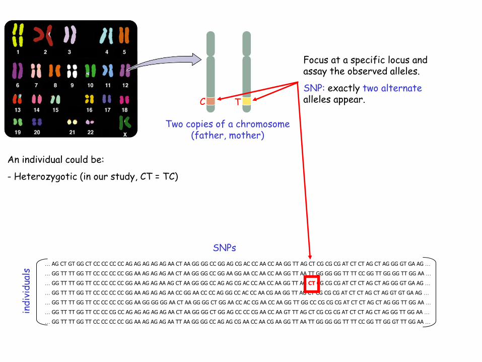
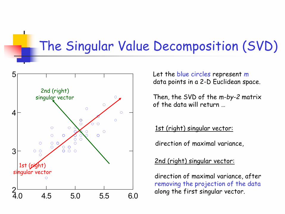
5 Let the blue circles represent mdata points in a 2-D Euclidean space.

Then, the SVD of the m-by-2 matrix of the data will return …

The Singular Value Decomposition (SVD)

4.0 4.5 5.0 5.5 6.02

3

4



1st (right) singular vector

1st (right) singular vector:

direction of maximal variance,


4.0 4.5 5.0 5.5 6.02

3

4




1st (right) singular vector:

direction of maximal variance,

2nd (right) singular vector

2nd (right) singular vector:

direction of maximal variance, after removing the projection of the dataalong the first singular vector.


4.0 4.5 5.0 5.5 6.02

3

4

5


2nd (right) singular vector

Singular values

σ1: measures how much of the data variance is explained by the first singular vector.

σ2: measures how much of the data variance is explained by the second singular vector.

σ1

σ2

Principal Components Analysis (PCA) is done via the computation of the Singular Value Decomposition (SVD) of a (mean-centered) covariance matrix.

Typically, a small constant number (say k) of the top singular vectors and values are kept.

SVD: formal definition

ρ: rank of A

U (V): orthogonal matrix containing the left (right) singular vectors of A.

Σ: diagonal matrix containing the singular values of A.

Let σ1 , σ2 , … , σρ be the entries of Σ.

Exact computation of the SVD takes O(min{mn2 , m2n}) time.

The top k left/right singular vectors/values can be computed faster using iterative methods.

0

0

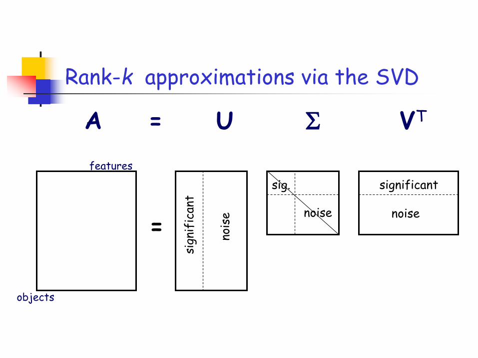
A VTΣU=

objects

features

significant

noiseno

ise noise

sign

ific

ant

sig.

=

Rank-k approximations via the SVD

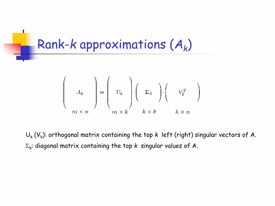
Rank-k approximations (Ak)

Uk (Vk): orthogonal matrix containing the top k left (right) singular vectors of A.

Σk: diagonal matrix containing the top k singular values of A.

HGDP data

• 1,033 samples


• 52 populations




The International HapMap Consortium (2003, 2005, 2007), Nature

Matrix dimensions:

2,240 subjects (rows)

447,143 SNPs (columns)The Human Genome Diversity Panel (HGDP)


CEU

TSIJPT, CHB, & CHD

GIH

MEX

HapMap Phase 3 data

• 1,207 samples

• 11 populations

HapMap Phase 3

SVD/PCA returns…

Africa

Middle East

South Central Asia

Europe

Oceania

East Asia

America

Gujarati Indians

Mexicans

• Top two Principal Components (eigenSNPs)

• Mexican population seems out of place: we move to the top three PCs.

Paschou, Lewis, Javed, & Drineas (2010) J Med Genet

AfricaMiddle East

S C Asia & Gujarati Europe

Oceania

East Asia

America

Not altogether satisfactory: the principal components are linear combinations of all SNPs, and – of course – can not be assayed!

Can we find actual SNPs that capture the information in the singular vectors?

Formally: spanning the same subspace.

Paschou, Lewis, Javed, & Drineas (2010) J Med Genet

Issues: computational time

Computing large SVDs: computational time• In commodity hardware (e.g., a 32GB RAM, i7 laptop), using MatLab R2021, the computation of the SVD of the dense 2,240-by-447,143 matrix A takes about 4 minutes.

• Computing this SVD is not a one-liner, since we (I?) could not load the whole matrix in RAM (runs out-of-memory in MatLab R2021); we compute the eigendecomposition of AAT.

• Current needs: we need to compute SVDs on biobank scale data (0.5M-1M samples genotyped on millions of SNPs).

Issues: computational time

Running time will always be a concern, but: we only need the top few principal components; machine-precision accuracy is not necessary!

• Data are noisy.

• Approximate singular vectors suffice.

Iterative methods with random starting points are well-explored in numerical linear algebra.

• Subspace iteration, Krylov subspace methods, etc.

• Careful implementations that scale are important.

Computing large SVDs: computational time• In commodity hardware (e.g., a 32GB RAM, i7 laptop), using MatLab R2021, the computation of the SVD of the dense 2,240-by-447,143 matrix A takes about 5 minutes.

• Computing this SVD is not a one-liner, since we (I?) could not load the whole matrix in RAM (runs out-of-memory in MatLab R2021); we compute the eigendecomposition of AAT.

• Current needs: we need to compute SVDs on biobank scale data (0.5M-1M samples genotyped on millions of SNPs).

Growing scale of Sequencing

Cost of sequencing and genotyping has gone down exponentially in recent years. Number of individuals sequenced has thus resulted in an exponential growth.

From the start of Human Genome project, to Human Genome Diversity Panel (1043 individuals, 660K SNPs) to now, UK Biobank having 500K individuals and ~95 million SNPs.

Biotech companies such as 23andMe, AncestryDNA, etc. have successfully sequenced around 2 million individuals and about 20-30 million (M) SNPs.

Bose et al. "TeraPCA: a fast and scalable software package to study genetic variation in tera-scale genotypes,“ Bioinformatics, 2019

Subspace Iteration: Methods

Subspace Iteration method is essentially a generalization of power method to approximate a 𝑘𝑘-dimensional 𝑘𝑘 > 1 invariant subspace, rather than one eigenvector at a time.

For a square matrix, 𝐵𝐵 ∈ ℝ𝑛𝑛×𝑛𝑛, a positive integer 𝑝𝑝 and a basis matrix 𝑋𝑋0 ∈ ℝ𝑛𝑛×𝑠𝑠 of an initial subspace, the subspace iteration computes the matrix: 𝑋𝑋 = 𝐵𝐵𝑝𝑝𝑋𝑋0.

𝑋𝑋0 is our initial guess matrix, for which we choose it to be random Gaussian vectors i.i.d from an 𝑁𝑁 0,1 distribution.

Given 𝐴𝐴 ∈ ℝ𝑚𝑚×𝑛𝑛,𝑋𝑋0 and 𝑝𝑝 , Subspace Iteration computes 𝑋𝑋 = 𝐴𝐴𝐴𝐴𝑇𝑇 𝑝𝑝𝑋𝑋0.

The problem is RAM, not running time…

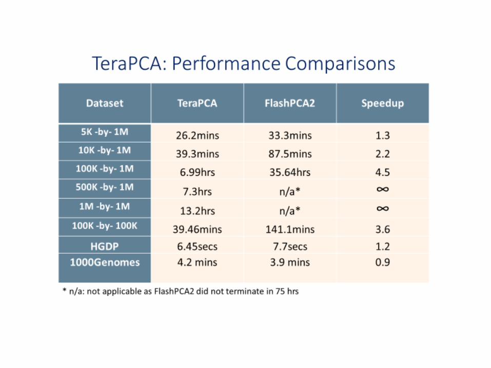
TeraPCA scales “decently” with increasing number of threads.(C++, MPI and multithreaded implementations using Intel’s OpenMP library)

Bose et al. "TeraPCA: a fast and scalable software package to study genetic variation in tera-scale genotypes,“ Bioinformatics, 2019

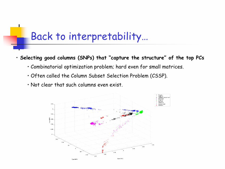
Back to interpretability…

• Selecting good columns (SNPs) that “capture the structure” of the top PCs

• Combinatorial optimization problem; hard even for small matrices.

• Often called the Column Subset Selection Problem (CSSP).

• Not clear that such columns even exist.

SVD decomposes a matrix as…

Top k left singular vectors

The SVD has strong optimality properties.

It is easy to see that X = ΣkVkT = Uk

TA.

SVD has strong optimality properties.

The columns of Uk are linear combinations of up to all columns of A.

The CX decompositionDrineas, Mahoney, & Muthukrishnan (2008) SIAM J Mat Anal ApplMahoney & Drineas (2009) PNAS

c columns of A

Carefully chosen X

Goal: make (some norm) of A-CX small.

Why?

If A is a subject-SNP matrix, then selecting representative columns is equivalent to selecting representative SNPs to capture the same structure as the top eigenSNPs.

We want c as small as possible!

CX decomposition

c columns of A

Easy to prove that optimal X = C+A. (C+ is the Moore-Penrose pseudoinverse of C.)

Thus, the challenging part is to find good columns (SNPs) of A to include in C.

From a mathematical perspective, this is a hard combinatorial problem, closely related to the so-called Column Subset Selection Problem (CSSP).

The CSSP has been heavily studied in Numerical Linear Algebra.

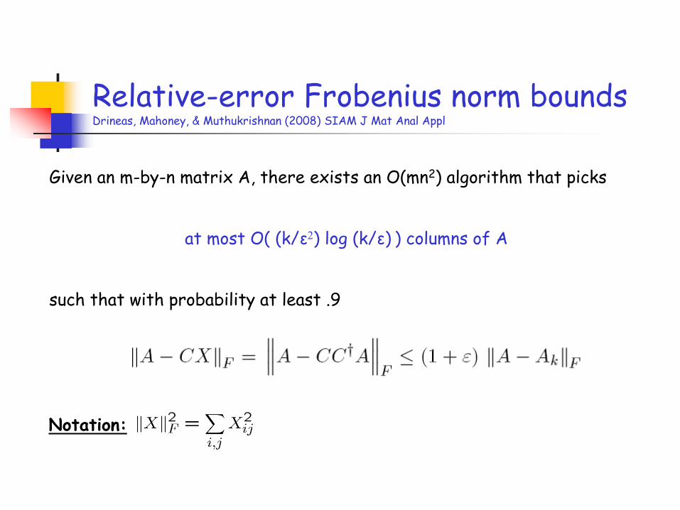
Relative-error Frobenius norm boundsDrineas, Mahoney, & Muthukrishnan (2008) SIAM J Mat Anal Appl

Given an m-by-n matrix A, there exists an O(mn2) algorithm that picks

at most O( (k/ε2) log (k/ε) ) columns of A

such that with probability at least .9

Notation:

The algorithm

Sampling algorithm

• Compute probabilities pj summing to 1.

• Let c = O( (k/ε2) log (k/ε) ).

• In c i.i.d. trials pick columns of A, where in each trial the j-th column of A is picked with probability pj.

• Let C be the matrix consisting of the chosen columns.

Input: m-by-n matrix A,

0 < ε < .5, the desired accuracy

Output: C, the matrix consisting of the selected columns

Subspace sampling (Frobenius norm)

Remark: The rows of VkT are orthonormal vectors, but its columns (Vk

T)(j) are not.

Vk: orthogonal matrix containing the top k right singular vectors of A.

Σ k: diagonal matrix containing the top k singular values of A.



T)(j) are not.

Subspace sampling in O(mn2) time



Normalization s.t. the pj sum up to 1



T)(j) are not.

Subspace sampling in O(mn2) time



Normalization s.t. the pj sum up to 1

Leverage scores(useful in statistics for

outlier detection)

Deterministic variant of CX

CX algorithm

• Compute the scores pj

• Pick the columns (SNPs) corresponding to the top c scores


integer k, and

c (number of SNPs to pick)

Output: the selected SNPs

Paschou et al (2007) PLoS Genetics

Mahoney and Drineas (2009) PNAS

CX algorithm


• Pick the columns (SNPs) corresponding to the top c scores


integer k, and

c (number of SNPs to pick)

Output: the selected SNPs: Ancestry Informative Markers

In order to estimate k for SNP data, we developed a permutation-based test to determine whether a certain principal component is significant or not.

(A similar test was presented in Patterson et al (2006) PLoS Genetics)

Paschou et al (2007) PLoS Genetics

Mahoney and Drineas (2009) PNAS

Deterministic variant of CX (cont’d)

-

Burunge

Mbuti

African Americans

Mende

Africa Europe

Spanish

European Americans

Chinese Japanese

E Asia

South Altaians-

America

Quechua

Nahua

274 individuals, 12 populations, ~10,000 SNPs using the Affymetrix array

Mala

Worldwide data

Puerto Rico

SNPs by chromosomal order

PCA

-sco

res

* top 30 PCA-correlated SNPs

Africa

Europe

Asia

America

Selecting PCA Informative SNPs for individual assignment to four continents (Africa, Europe, Asia, America)

Paschou et al (2007; 2008) PLoS Genetics; Paschou et al (2010) J Med Genet; Drineas et al (2010) PLoS One

Hughey, Paschou, Drineas, et al. (2013) Nat Comm; Paschou, Drineas, et al. PNAS 2014;

SNPs by chromosomal order

PCA

-sco

res

* top 30 PCA-correlated SNPs

Africa

Europe

Asia

America

Afr

Eur

Asi

Ame

Selecting PCA Informative SNPs for individual assignment to four continents (Africa, Europe, Asia, America)

Paschou et al (2007; 2008) PLoS Genetics; Paschou et al (2010) J Med Genet; Drineas et al (2010) PLoS One

Hughey, Paschou, Drineas, et al. (2013) Nat Comm; Paschou, Drineas, et al. PNAS 2014;

A large world-wide sample: ALFRED data (K.K. Kidd’s lab @ Yale)

A total of 3,567 samples from 92 populations and 442,516 common SNPs

Africa

America

Europe

East Asia

OceaniaCS Asia

SW Asia

Mexican

Gene Function (RefSeq)

EDAR* Ectodermal development, hair follicle formation.

PTK6 Intracellular signal transducer in epithelial tissues. Sensitization of cells to epidermal growth factor.

SPATA20* Associated with spermatogenesis.

MCHR1 Plasma membrane protein which binds melanin-concentrating hormone. Probably involved in the neuronal regulation of food consumption.

FOXP1* Forkhead box transcription factors play important roles in the regulation of tissue- and cell type-specific gene transcription during both development and adulthood.

PSCD3* Involved in the control of Golgi structure and function.

OCA2* Skin/Hair/Eye pigmentation.

EGFR* This protein is a receptor for members of the epidermal growth factor family.Associated with the melanin pathway.

Highest scoring “genes”

*Barreiro et al (2008) Nat Genet

*Sabeti et al (2007) Nature

*The International HapMap Consortium (2007) Nature

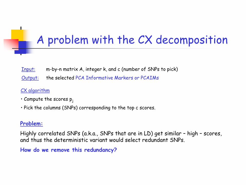
A problem with the CX decomposition

CX algorithm


• Pick the columns (SNPs) corresponding to the top c scores.

Input: m-by-n matrix A, integer k, and c (number of SNPs to pick)

Output: the selected PCA Informative Markers or PCAIMs

Problem:

Highly correlated SNPs (a.k.a., SNPs that are in LD) get similar – high – scores, and thus the deterministic variant would select redundant SNPs.

How do we remove this redundancy?

Rank-Revealing QR factorizationPaschou et al (2008) PLoS GeneticsBoutsidis, Mahoney, & Drineas (2009) SODA

We use a standard greedy approach (the Rank-Revealing QR factorization).

The algorithm performs k iterations:

In the first iteration, the top PCAIM is picked;

In the second iteration, a PCAIM is picked that is as uncorrelated to with the previously selected PCAIM as possible;

In the third iteration the chosen PCAIM has to be as uncorrelated as possiblewith the first two previously selected PCAIMs;

And so on…Efficient implementations are available, and run in a couple of minutes for typical values of m, c, and k.

Problem

How many columns do we need to include in the matrix C in order to get relative-error approximations ?

Recall: with O( (k/ε2) log (k/ε) ) columns, we get (subject to a failure probability)

Deshpande & Rademacher (FOCS ’10): with exactly k columns, we get

What about the range between k and O(k log(k))?

Selecting fewer columns

Selecting fewer columns (cont’d)(Boutsidis, Drineas, & Magdon-Ismail, FOCS 2011 and SICOMP 2014)

Question:

What about the range between k and O(k log(k))?

Answer:

A relative-error bound is possible by selecting s=2k/ε columns!

Technical breakthrough;

A combination of sampling strategies with a novel approach on column selection, inspired by the work of Batson, Spielman, & Srivastava (STOC ’09) on graph sparsifiers.

• The running time is O((mnk+nk3)ε-1).

• Simplicity is gone…

CSSP: Lower bounds & other approachesGuruswami & Sinop, SODA 2012

Alternative approaches, based on volume sampling, guarantee

(r+1)/(r+1-k) relative error bounds.

This bound is asymptotically optimal (up to lower order terms).

The proposed deterministic algorithm runs in O(rnm3 log m) time, while the randomized algorithm runs in O(rnm2) time and achieves the bound in expectation.

Guruswami & Sinop, FOCS 2011

Applications of column-based reconstruction in Quadratic Integer Programming.

Very large body of followup work in the Theoretical Computer Science

CSSPMassive body of follow-up work on the CSSP, including the NeurIPS 2020 best paper award for:

Michal Derezinski, Rajiv Khanna, Michael W. Mahoney, “Improved guarantees and a multiple-descent curve for the Column Subset Selection Problem and the Nyströmmethod”, NeurIPS 2020.

(See discussion and references in the above paper for a summary of theoretical and applied work on the CSSP.)

We also use genetics analyses to elucidate population relationships and provide answers to historical questions of relevance to archeology and paleoanthropology.

Again, PCA plots are quite telling.

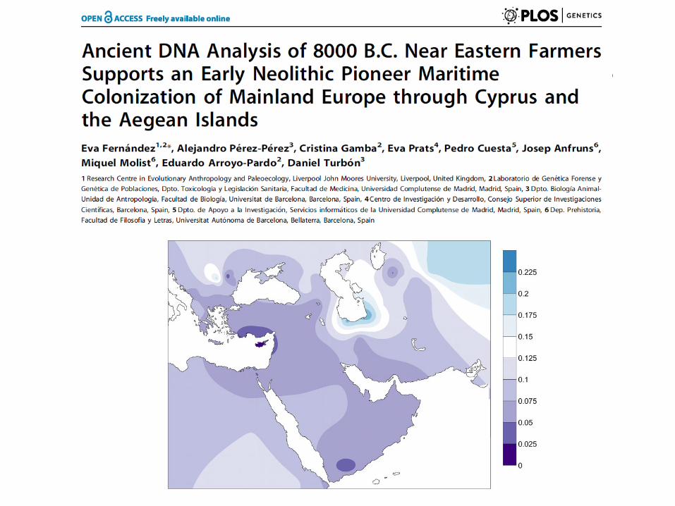
Multiple examples from our own work:• A maritime path for the colonization of Europe.

(Paschou et al. PNAS 2014)

• The origins of the Minoan civilization.(Hughey et al. Nat Comms 2013)

• Disproving Fallmerayer’s hypothesis (~1830s) that Byzantine and medieval Greeks (esp. Peloponneseans) were extinguished by Slavic invaders and replaced by Slavic settlers during the 6th century CE.

(Stamatoyannopoulos et al. Eur J Hum Gen 2017; Drineas et al. Hum Gen 2019)

We started collecting data to investigate these hypotheses since 2011; joint work with P. Paschou (Purdue), J. Stamatoyannopoulos (U Washington), and G. Stamatoyannopoulos (U Washington).

Greece at the crossroads of Neolithic migrations into Europe

• Possible routes of migration:• Anatolia to Bosporus to

Thrace



Thrace• Maritime route from the

coast of Anatolia to the Aegean islands to Southeast Europe



Thrace• Maritime route from the

coast of Anatolia to the Aegean islands to Southeast Europe

• Middle East to the Aegean to Europe

The Data

964 samples from 32 populations genotyped across 75,194 SNPs across all autosomes•Crete, Dodecanese (Aegean islands)

•3 populations from mainland Greece

•Cappadocia (Anatolia)

•14 populations from Northern and Southern Europe

•7 populations from North Africa

•5 populations from Middle East

Population genetic structure around the Mediterranean

The Mediterranean as a barrier in gene flow

Analysis using BARRIER software (combination of genetic and geographic

distances)

North Africa

Middle East

Cappadocia

CretePeloponnese

Northern Europe

Constructing gene flow networks

The islands of Crete and the Dodecanese as a bridge connecting Anatolia to the Southern Peloponnese and the rest of Europe

Neolithic migrations to Europe via a maritime route

• The islands of the Aegean and Crete are important nodes of migration towards Europe in the Neolithic Era.

• The Mediterranean acted as a barrier for migrations to Europe from Northern Africa.

Paschou, Drineas, et al. PNAS 2014

What about India?

Bose et al. "Integrating linguistics, social structure, and geography to model genetic diversity within India,“ Mol Bio & Evo, 2021

For more details: Bose et al. Mol Bio & Evo (2021)

Open questions

Unsupervised dimensionality reduction techniques are NOT successful in separating cases from controls in GWAS studies.

Why? Because the disease signal is too “weak”.

Potential remedies? Supervised techniques, e.g., GLMs, SVMs, Deep Learning, etc.

Goal? Supervised dimensionality reduction techniques that identify axes that separate cases from controls. Then, identify SNPs (and genes) that span the same subspace as those axes.

Looks challenging, especially if the objective is to separate cases and controls (too stringent).

Maybe relax the objective? Separating averages is too naïve; is there something more interesting?

AcknowledgementsCollaborators

P. Paschou, PurdueE. Ziv, UCSFK. K. Kidd, Yale UniversityM. W. Mahoney, UC BerkeleyJ. Stamatoyannopoulos, U WashingtonG. Stamatoyannopoulos, U Washington

Students

A. Javed, RPIJ. Lewis, RPIJ. Alexander, RPIA. Bose, PurdueF. Tsetsos, PurdueM. Burch, PurdueP. Jain, PurdueZ. Yang, Purdue

Funding: NSF, NIH, DOE, EMBO, IBM, Tourette Syndrome Association, EU FP7 Programme.

Papers and preprints: google Drineas; go to Publications page.

Documents

Dimensionality Reduction in the Analysis of Human Genetics