Dimensionality reduction for acoustic vehicleclassification with spectral embedding

Justin SunuInstitute of Mathematical Sciences

Claremont Graduate UniversityClaremont, CA 91711

Email: justinsunu@gmail.com

Allon G. PercusInstitute of Mathematical Sciences

Claremont Graduate UniversityClaremont, CA 91711

Email: allon.percus@cgu.edu

Abstract—We propose a method for recognizing moving vehi-cles, using data from roadside audio sensors. This problem hasapplications ranging widely, from traffic analysis to surveillance.We extract a frequency signature from the audio signal usinga short-time Fourier transform, and treat each time window asan individual data point to be classified. By applying a spectralembedding, we decrease the dimensionality of the data sufficientlyfor K-nearest neighbors to provide accurate vehicle identification.

I. INTRODUCTION

Classification and identification of moving vehicles fromaudio signals is of interest in many applications, ranging fromtraffic flow management to military target recognition. Clas-sification may involve differentiating vehicles by type, suchas jeep, sedan, etc. Identification can involve distinguishingspecific vehicles, even within a given vehicle type.

Since audio data is small compared to, say, video data,multiple audio sensors can be placed easily and inexpensively.However, there are certain obstacles having to do with bothhardware and physics. Certain microphones and recording de-vices have built-in features, for example, damping/normalizingthat may be applied when the recording exceeds a threshold.Microphone sensitivity is another equipment problem: theslightest wind could give disruptive readings that affect theanalysis. Ambient noise is a further issue, adding perturbationsto the signal. Physical challenges include the Doppler shift,where the sound of a vehicle approaching differs from thesound of it leaving, so trying to relate these two can provedifficult.

The short-time Fourier transform (STFT) is often used forfeature extraction in audio signals. We adopt this approach,choosing time windows large enough that they carry sufficientfrequency information but small enough that they allow us tolocalize vehicle events. Afterwards, we use spectral embeddingas a dimension reduction technique, reducing from thousandsof Fourier coefficients to a small number of graph Laplacianeigenvectors. We then cluster the low-dimensional data usingK-means, establishing an unsupervised spectral clusteringbaseline prediction. Finally, we improve upon this by usingK-nearest neighbors as a simple but highly effective formof semi-supervised learning, giving an accurate classification

without the need for large quantities of training data requiredby frequently used supervised approaches such as deep learn-ing.

In this paper, we apply these methods to audio recordingsof passing vehicles. In Section 2, we provide background onvehicle classification using audio signals. In Section 3, wediscuss the characteristics of the vehicle data that we use.Section 4 describes our feature extraction methods. Section5 discusses our classification methods. Section 6 presents ourresults. We conclude in section 7 with a discussion of ourmethod’s strengths and limitations, as well as future directions.

II. BACKGROUND

The vast majority of the literature in audio classification isdevoted to speech and music processing, with relatively fewpapers on problems of vehicle identification and classification.The most closely related work has included using principlecomponent analysis for classifying car vs. motorcycle [1],using an ε-neighborhood to cluster Fourier coefficients to clas-sify different vehicles [2], and using both the power spectraldensity and wavelet transform with K-nearest neighbors andsupport vector machines to classify vehicles [3]. Our studytakes a graph-based clustering approach to identifying differentindividual vehicles from their Fourier coefficients.

Analyzing audio data generally involves the following steps:

1) Preprocess raw data.2) Extract features in data.3) Process extracted data.4) Analyze processed data.

The most common form of preprocessing on raw data is en-suring that it has zero mean, by subtracting any bias introducedin the sound recording [2], [3]. Another form of preprocessingis applying a weighted window filter to the raw data. Forexample, the Hamming window filter is often used to reducethe effects of jump discontinuity when applying the short-time Fourier transform, known as the Gibbs’ effect [1]. Thefinal preprocessing step deals with the manipulation of datasize, namely how to group audio frames into larger windows.Different window sizes have been used in the literature, withno clear set standard. Additionally, having some degree of

arX

iv:1

705.

0986

9v2

[st

at.M

L]

17

Feb

2018

overlap between successive windows can help smooth results[1]. The basis for these preprocessing steps is to set up thedata to allow for better feature extraction.

STFT is frequently used for feature extraction [1], [2], [3],[4]. Other approaches include the wavelet transform [3], [5]and the one-third-octave filter bands [6]. All of these methodsaim at extracting underlying information contained within theaudio data.

After extracting pertinent features, additional processing isneeded. When working with STFT, the amplitudes for theFourier coefficients are generally normalized before analysis isperformed [1], [2], [3], [4]. Another processing step applied tothe extracted features is dimension reduction [7]. The Fouriertransform results in a large number of coefficients, giving ahigh-dimensional description of the data. We use a spectralembedding to reduce the dimensionality of the data [8]. Thespectral embedding requires the use of a distance function onthe data points: by adopting the cosine distance, we avoid theneed for explicit normalization of the Fourier coefficients.

Finally, the analysis of the processed data involves theclassification algorithm. Methods used for this have includedthe following:

• K-means and K-nearest neighbors [3]• Support vector machines [3]• Within ε distance [2]• Neural networks [6]

K-means and K-nearest neighbors are standard techniquesfor analyzing the graph Laplacian eigenvectors resulting fromspectral clustering [8]. They are among the simplest methods,but are also well suited to clustering points in the low-dimensional space obtained through the dimensionality reduc-tion step.

III. DATA

Our dataset consists of recordings, provided by the USNavy’s Naval Air Systems Command [9], of different vehiclesmoving multiple times through a parking lot at approximately15mph. While the original dataset consists of MP4 videostaken from a roadside camera, we extract the dual channelaudio signal, and average the channels together into a singlechannel. The audio signal has a sampling rate of 48,000 framesper second. Video information is used to ascertain the groundtruth (vehicle identification) for training data.

The raw audio signal already has zero mean. Therefore, theonly necessary preprocessing is grouping audio frames intotime windows for STFT. We found that with windows of 1/8of a second, or 6000 frames, there is both a sufficient numberof windows and sufficient information per window. This iscomparable to window sizes used in other studies [1].

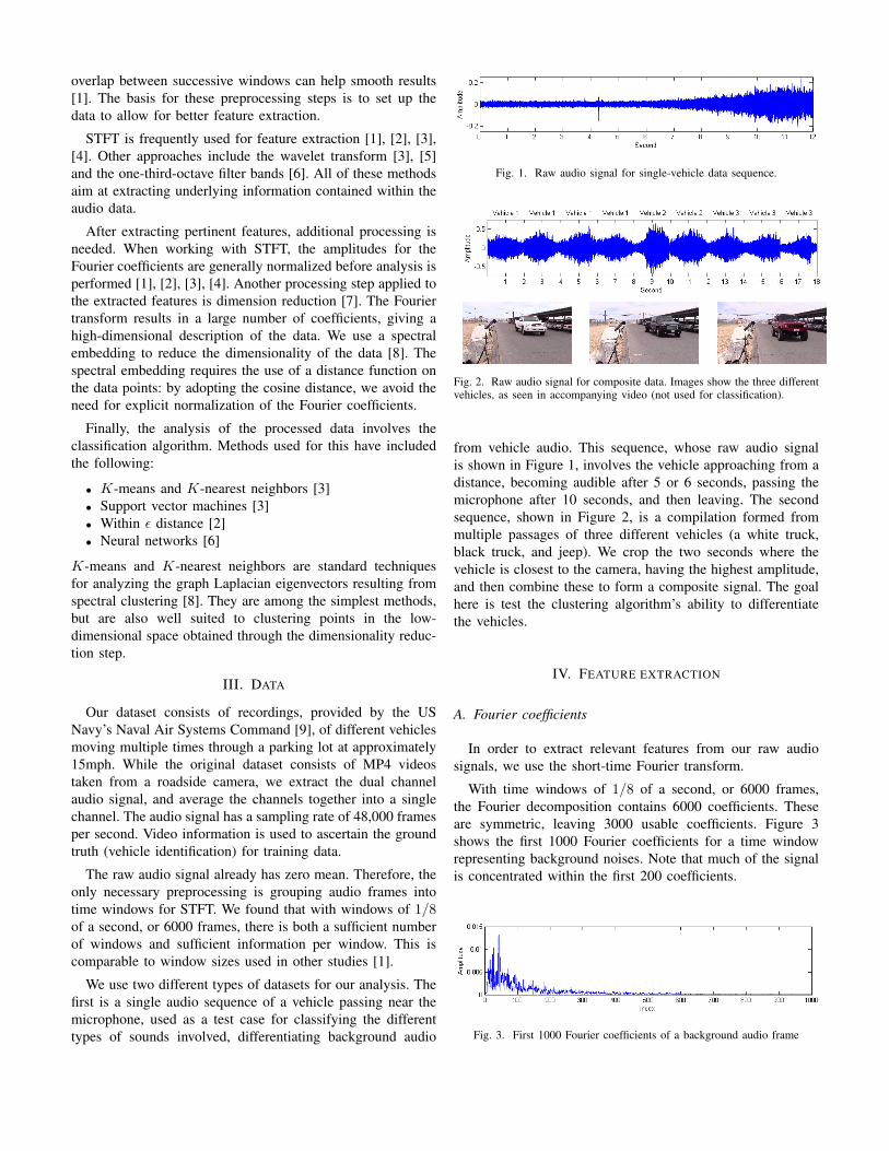
We use two different types of datasets for our analysis. Thefirst is a single audio sequence of a vehicle passing near themicrophone, used as a test case for classifying the differenttypes of sounds involved, differentiating background audio

Fig. 1. Raw audio signal for single-vehicle data sequence.

Fig. 2. Raw audio signal for composite data. Images show the three differentvehicles, as seen in accompanying video (not used for classification).

from vehicle audio. This sequence, whose raw audio signalis shown in Figure 1, involves the vehicle approaching from adistance, becoming audible after 5 or 6 seconds, passing themicrophone after 10 seconds, and then leaving. The secondsequence, shown in Figure 2, is a compilation formed frommultiple passages of three different vehicles (a white truck,black truck, and jeep). We crop the two seconds where thevehicle is closest to the camera, having the highest amplitude,and then combine these to form a composite signal. The goalhere is test the clustering algorithm’s ability to differentiatethe vehicles.

IV. FEATURE EXTRACTION

A. Fourier coefficients

In order to extract relevant features from our raw audiosignals, we use the short-time Fourier transform.

With time windows of 1/8 of a second, or 6000 frames,the Fourier decomposition contains 6000 coefficients. Theseare symmetric, leaving 3000 usable coefficients. Figure 3shows the first 1000 Fourier coefficients for a time windowrepresenting background noises. Note that much of the signalis concentrated within the first 200 coefficients.

Fig. 3. First 1000 Fourier coefficients of a background audio frame

B. Fourier reconstructions

Given the concentration of frequencies, we hypothesize thatwe can isolate specific sounds by selecting certain ranges offrequency. To test this, we perform a reconstruction analysisof the Fourier coefficients. After performing the Fourier trans-form, we zero out a certain range of Fourier coefficients andthen perform the inverse Fourier transform. This has the effectof filtering out the corresponding range of frequencies.

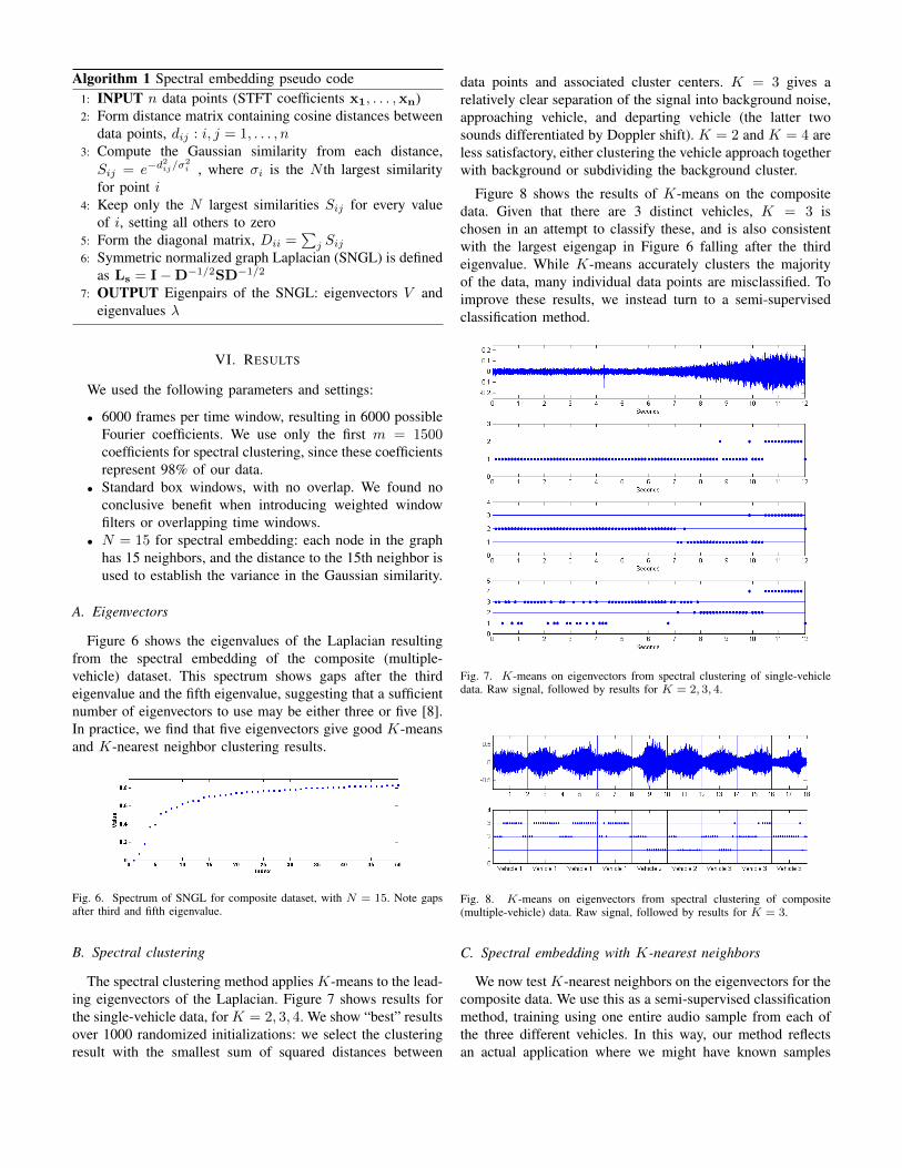
Figure 4 shows the results of the reconstruction on anaudio recording exhibiting strong wind sounds for the first12 seconds, before the arrival of the vehicle at second 14.In a) the raw signal is shown. In b) we keep only the first130 coefficients, in c) we keep only the next 130 coefficients,and in d) we keep all the rest of the coefficients. We seein the reconstruction that the first 130 Fourier coefficientscontain most of the background sounds, including the strongwind that corresponds to the large raw signal amplitudesin the first 12 seconds. The remaining Fourier coefficientsare largely insignificant during this time. When the vehiclebecomes audible, however, the second 130 and the rest of thecoefficients exhibit a significant increase in amplitude.

By listening to the audio of the reconstructions b) throughd), one can confirm that the first 130 coefficients primarilyrepresent the background noise, while the second 130 and therest of the audio capture most of the sounds of the movingvehicle. This suggests that further analysis into the detectionof background frame signatures could yield a better methodfor finding which frequencies to filter out, in order to yieldbetter reconstructed audio sequences.

a) Raw signal data.

b) Reconstruction using first 130 Fourier coefficients.

c) Reconstruction using second 130 Fourier coefficients.

d) Reconstruction using remaining Fourier coefficients.Fig. 4. Decomposition of an additional (single-vehicle) data sequence intothree frequency bands.

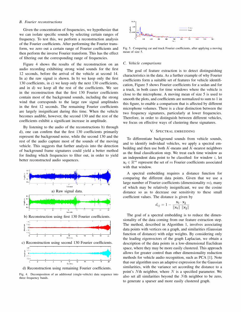
Fig. 5. Comparing car and truck Fourier coefficients, after applying a movingmean of size 5.

C. Vehicle comparisons

The goal of feature extraction is to detect distinguishingcharacteristics in the data. As a further example of why Fouriercoefficients form a suitable set of features for vehicle identifi-cation, Figure 5 shows Fourier coefficients for a sedan and fora truck, in both cases for time windows where the vehicle isclose to the microphone. A moving mean of size 5 is used tosmooth the plots, and coefficients are normalized to sum to 1 inthis figure, to enable a comparison that is affected by differentmicrophone volumes. There is a clear distinction between thetwo frequency signatures, particularly at lower frequencies.Therefore, in order to distinguish between different vehicles,we focus on effective ways of clustering these signatures.

V. SPECTRAL EMBEDDING

To differentiate background sounds from vehicle sounds,and to identify individual vehicles, we apply a spectral em-bedding and then use both K-means and K-nearest neighborsas the final classification step. We treat each time window asan independent data point to be classified: for window i, letxi ∈ Rm represent the set of m Fourier coefficients associatedwith that window.

A spectral embedding requires a distance function forcomparing the different data points. Given that we use alarge number of Fourier coefficients (dimensionality m), manyof which may be relatively insignificant, we use the cosinedistance so as to decrease our sensitivity to these smallcoefficient values. The distance is given by

dij = 1− xi · xj

‖xi‖ ‖xj‖

The goal of a spectral embedding is to reduce the dimen-sionality of the data coming from our feature extraction step.The method, described in Algorithm 1, involves associatingdata points with vertices on a graph, and similarities (Gaussianfunction of distance) with edge weights. By considering onlythe leading eigenvectors of the graph Laplacian, we obtain adescription of the data points in a low-dimensional Euclideanspace, where they may be more easily clustered. This approachallows for greater control than other dimensionality reductionmethods for vehicle audio recognition, such as PCA [1]. Notethat our algorithm uses an adaptive expression for the Gaussiansimilarities, with the variance set according the distance to apoint’s N th neighbor, where N is a specified parameter. Wealso set all similarities beyond the N th neighbor to be zero,to generate a sparser and more easily clustered graph.

Algorithm 1 Spectral embedding pseudo code1: INPUT n data points (STFT coefficients x1, . . . ,xn)2: Form distance matrix containing cosine distances between

data points, dij : i, j = 1, . . . , n3: Compute the Gaussian similarity from each distance,Sij = e−d

2ij/σ

2i , where σi is the N th largest similarity

for point i4: Keep only the N largest similarities Sij for every value

of i, setting all others to zero5: Form the diagonal matrix, Dii =

∑j Sij

6: Symmetric normalized graph Laplacian (SNGL) is definedas Ls = I−D−1/2SD−1/2

7: OUTPUT Eigenpairs of the SNGL: eigenvectors V andeigenvalues λ

VI. RESULTS

We used the following parameters and settings:

• 6000 frames per time window, resulting in 6000 possibleFourier coefficients. We use only the first m = 1500coefficients for spectral clustering, since these coefficientsrepresent 98% of our data.

• Standard box windows, with no overlap. We found noconclusive benefit when introducing weighted windowfilters or overlapping time windows.

• N = 15 for spectral embedding: each node in the graphhas 15 neighbors, and the distance to the 15th neighbor isused to establish the variance in the Gaussian similarity.

A. Eigenvectors

Figure 6 shows the eigenvalues of the Laplacian resultingfrom the spectral embedding of the composite (multiple-vehicle) dataset. This spectrum shows gaps after the thirdeigenvalue and the fifth eigenvalue, suggesting that a sufficientnumber of eigenvectors to use may be either three or five [8].In practice, we find that five eigenvectors give good K-meansand K-nearest neighbor clustering results.

Fig. 6. Spectrum of SNGL for composite dataset, with N = 15. Note gapsafter third and fifth eigenvalue.

B. Spectral clustering

The spectral clustering method applies K-means to the lead-ing eigenvectors of the Laplacian. Figure 7 shows results forthe single-vehicle data, for K = 2, 3, 4. We show “best” resultsover 1000 randomized initializations: we select the clusteringresult with the smallest sum of squared distances between

data points and associated cluster centers. K = 3 gives arelatively clear separation of the signal into background noise,approaching vehicle, and departing vehicle (the latter twosounds differentiated by Doppler shift). K = 2 and K = 4 areless satisfactory, either clustering the vehicle approach togetherwith background or subdividing the background cluster.

Figure 8 shows the results of K-means on the compositedata. Given that there are 3 distinct vehicles, K = 3 ischosen in an attempt to classify these, and is also consistentwith the largest eigengap in Figure 6 falling after the thirdeigenvalue. While K-means accurately clusters the majorityof the data, many individual data points are misclassified. Toimprove these results, we instead turn to a semi-supervisedclassification method.

Fig. 7. K-means on eigenvectors from spectral clustering of single-vehicledata. Raw signal, followed by results for K = 2, 3, 4.

Fig. 8. K-means on eigenvectors from spectral clustering of composite(multiple-vehicle) data. Raw signal, followed by results for K = 3.

C. Spectral embedding with K-nearest neighbors

We now test K-nearest neighbors on the eigenvectors for thecomposite data. We use this as a semi-supervised classificationmethod, training using one entire audio sample from each ofthe three different vehicles. In this way, our method reflectsan actual application where we might have known samples

of vehicles. The results for K = 16 are shown in Figure9. The corresponding confusion matrix is given in Table I.We allow for training points to be classified outside of theirown class (seen in the case of vehicle 3), allowing for abetter evaluation of the method’s accuracy. While a few datapoints are misclassified, the vast majority (88.2%) are correct.Training on an entire vehicle passage appears sufficient toovercome Doppler shift effects in our data: the approachingsounds and departing sounds of a given vehicle are correctlyplaced in the same class.

Fig. 9. K-nearest neighbors on eigenvectors from spectral embedding ofcomposite (multiple-vehicle) data, for K = 15. Training points are shownwith red circles. Shaded regions show correct classification.

TABLE ICLASSIFICATION RESULTS FOR K-NEAREST NEIGHBOR.

TrueObtained Vehicle 1

(white truck)Vehicle 2

(black truck)Vehicle 3

(jeep)Vehicle 1 (white truck) 64 0 0Vehicle 2 (black truck) 1 30 1

Vehicle 3 (jeep) 11 4 33

VII. CONCLUSIONS

Identifying moving vehicles from audio recordings is achallenging and broadly applicable problem. We have demon-strated an approach that classifies frequency signatures, apply-ing the short-time Fourier transform (STFT) to the audio signaland describing the sound at each 1/8-second time windowusing 1500 Fourier coefficients. Using a spectral embedding,we reduce the dimensionality of the data from 1500 to 5,corresponding to the five eigenvectors of the graph Laplacian.K-nearest neighbors then associates vehicle sounds with thecorrect vehicle in 88.2% of the time windows in our test data.

Our analysis treats time windows as independent datapoints, and therefore ignores temporal correlations. It ispossible that we could improve results by explicitly incor-porating time information into our classification algorithm.For instance, one straightforward approach could be to useas data points a sliding window of larger width. In somecases, however, ignoring time information could actually helpour method, for instance by helping the classifier correctlyassociate the Doppler-shifted sounds of a given vehicle ap-proaching and departing.

A limitation of our study is that our audio samples onlyinvolve single vehicles, under relatively tightly controlledconditions. The presence of multiple vehicles, or significantexternal noise such as in an urban environment, would pose achallenge to our feature extraction method. While the STFT isstandard in audio processing, the use of time windows imposesa specific time scale that may not always be appropriate.Furthermore, the Fourier decomposition may be insufficientlysparse, with too many distinct Fourier components present invehicle audio signals. To overcome these difficulties, one coulduse multiscale techniques such as wavelet decompositions thathave been proposed for vehicle detection and classification [3],[5]. More recently developed sparse decomposition methodsmay also be of use, as they implicitly learn a good choice ofbasis functions from the data [10], [11], [12], [13].

An additional area for improvement is our clustering al-gorithm. More sophisticated methods than K-means and K-nearest neighbors may allow for vehicle identification underless tightly controlled conditions than those in our experi-ments, or possibly for identifying broad types of vehicles suchas cars or trucks. Such semi-supervised methods would pre-serve the chief benefit of our approach, namely its applicabilityin cases where only very limited training data are available.

REFERENCES

[1] H. Wu, M. Siegel, and P. Khosla, “Vehicle sound signature recognitionby frequency vector principle component analysis,” IEEE Transactionson Instrumentation and Measurement, vol. 48, 1999.

[2] S. S. Yang, Y. G. Kim, and H. Choi, “Vehicle identification usingwireless sensor networks,” IEEE SoutheastCon, 2007.

[3] A. Aljaafreh and L. Dong, “An evaluation of feature extraction methodsfor vehicle classification based on acoustic signals,” IEEE InternationalConference on Networking, Sensing and Control, 2010.

[4] S. Kozhisseri and M. Bikdash, “Spectral features for the classificationof civilian vehicles using acoustic sensors,” IEEE Workshop on Compu-tational Intelligence in Vehicles and Vehicular Systems, 2009.

[5] A. Averbuch, V. A. Zheludev, N. Rabin, and A. Schclar, “Wavelet-basedacoustic detection of moving vehicles,” Multidimensional Systems andSignal Processing, 2009.

[6] N. A. Rahim, P. M. P, A. H. Adom, and S. S. Kumar, “Moving vehiclenoise classification using multiple classifiers,” IEEE Student Conferenceon Research and Development, 2011.

[7] A. Averbuch, N. Rabin, A. Schclar, and V. Zheludev, “Dimensionalityreduction for detection of moving vehicles,” Pattern Analysis andApplications, 2012.

[8] U. V. Luxburg, “A tutorial on spectral clustering,” Statistics and com-puting, 2007.

[9] A. Flenner, personal communication.[10] I. Daubechies, J. Lu, and H.-T. Wu, “Synchrosqueezed wavelet

transforms: An empirical mode decomposition-like tool,” Applied andComputational Harmonic Analysis, vol. 30, no. 2, pp. 243 – 261,2011. [Online]. Available: http://www.sciencedirect.com/science/article/pii/S1063520310001016

[11] T. Y. Hou and Z. Shi, “Adaptive data analysis via sparse time-frequency representation,” Advances in Adaptive Data Analysis,vol. 03, no. 01n02, pp. 1–28, 2011. [Online]. Available: http://www.worldscientific.com/doi/abs/10.1142/S1793536911000647

[12] J. Gilles, “Empirical wavelet transform,” IEEE Transactions on SignalProcessing, vol. 61, no. 16, pp. 3999–4010, Aug 2013.

[13] C. K. Chui and H. Mhaskar, “Signal decomposition and analysisvia extraction of frequencies,” Applied and Computational HarmonicAnalysis, vol. 40, no. 1, pp. 97 – 136, 2016. [Online]. Available:http://www.sciencedirect.com/science/article/pii/S1063520315000044