Dimensional Analysis in Economics

7/27/2019 Dimensional Analysis in Economics

http://slidepdf.com/reader/full/dimensional-analysis-in-economics 1/21

R OGER NILS FOLSOM is professor emeritus of economics and R ODOLFO A LEJO GONZALEZ isprofessor of economics at San Jose State University. Our thanks go to Ann Arlene MarquissFolsom for editing; an anonymous referee for showing us the need to reorganize for betterclarity; Mario Roque Escobar for help in streamlining our macroeconomic model discus-sion; Tom Means for clarifying our understanding of an “independently and identicallydistributed (i.i.d.) process,” and Edward Stringham and Benjamin Powell for other sug-gestions. The authors remain responsible for any existing errors.

1This inattention to dimensional analysis begins with introductory economics (andbusiness) textbooks, in which function examples usually ignore dimensions. For example,textbooks routinely include demand and supply functions such as q d = 10 - 3 p or q s = 2 +5 p , with no mention that 10, -3, 2, and 5 all are parameter values that must have dimen-sions, such that the function’s left side dimension is matched by the function’s right sidedimension. In this case, the dependent variable has quantity dimension “quantity unit”(e.g., bushels), and the independent variable has price dimension “monetary unit / quan-tity unit” (e.g., dollars/bushel). Hence the freestanding additive parameters 10 or 2 eachmust have the dimension “quantity unit,” and the (logical) slope parameters -3 or 5 eachmust have the dimension “(quantity unit)2 / monetary unit.” Far better is to introducefunctions in a more general form, such as q d = D ( p ) = d 0 + d 1 p (where d 1 < 0) and q s =S ( p ) = s 0 + s 1 p , and then discuss parameter dimensions and suggest reasonable parame-ter values.

DIMENSIONS AND ECONOMICS:SOME A NSWERS

R OGER NILS FOLSOM AND R ODOLFO A LEJO GONZALEZ

W

illiam Barnett’s (2004) critique of mathematics in economic analy-sis, “Dimensions and Economics: Some Problems,” claims that

economics almost always uses functions and equations withoutpaying any attention to their variable and parameter dimensions and units. Bycasual observation, that criticism appears often to be true,1 and it applies notonly to functions and equations but also to relations of all sorts, includinginequalities.

Following his introduction, Barnett (p. 95) makes his main case in threesections, using two different examples: The Cobb-Douglas production func-tion, whose parameters he sees as having (1) “meaningless or economicallyunreasonable dimensions” (p. 96) and (2) “inconstant” dimensions (p. 97). A macroeconomic model, whose technology (production) function’s parameters

THE QUARTERLY JOURNAL OF AUSTRIAN ECONOMICS VOL. 8, NO. 4 (WINTER 2005): 45–65

45



he sees as either (3) “meaningless,” or else as defining a function that relatesoutput hours to labor input hours, which yields “no net production.” Either

way, the model is “not defensible” (pp. 97–98).

Professor Barnett’s fourth and fifth sections, “Discussion” (pp. 98–99) and“Conclusions” (p. 99), state that

[Modern economics’] failure to use dimensions consistently and correctlyin production [and other economic] functions . . . are both critical andubiquitous—they afflict virtually all mathematical and econometric mod-els of economic activity. . . . [T]he failure to use dimensions consistentlyand correctly . . . render the models so afflicted virtually worthless. . . .

[Economics has been “emulating” the methods of “physicists and engi-neers,” but has “failed to emulate” them in] the consistent and correct useof dimensions. This is an abuse of mathematical/scientific methods. Suchabuse invalidates the results of mathematical and statistical methodsapplied to the development and application of economic theory. . . . [I]t is

a continuing problem and one found in the leading mainstream journals(and textbooks). . . . [U]nless and until this changes, and economists con-sistently and correctly use dimensions in economics, if such is possible,mathematical economics, and its empirical alter ego, econometrics, willcontinue to be academic games and “rigorous” pseudosciences. . . .

This is not to say that there have not been advances in economic under-standing by the neoclassicals, but rather to argue that mathematics is nei-ther a necessary nor a sufficient means to such advances. Whether it evenis, or can be, a valid means to such advances is a different issue.

Professor Barnett makes some good points in his critique of the use of mathematics in economics. Criticism of mathematical economics, however, ishardly a novel topic among Austrian economists (Mises 1977; 1966, pp.

350–57).2 And the misuse and abuse of mathematics in contemporary eco-nomics has been noticed, denounced, and lamented even by prominent main-stream economists (see Blaug 1998, pp. 11–34, and his citations). What isnovel in Barnett’s article is his claim that dimensional errors in the mathe-matical functions used in economics are “ubiquitous,” which makes a lot of mainstream economic models “worthless.” Although much and perhaps mostcontemporary neoclassical economics may be worthless, that assessment haslong preceded Barnett’s dimensional issue.

In our judgment, Barnett’s discussion of the Cobb-Douglas productionfunction and of the macroeconomic model merits further examination. Thateconomics often ignores dimensions and units does not necessarily mean thatunstated but implied dimensions and units are wrong or invalid.

46 THE QUARTERLY JOURNAL OF AUSTRIAN ECONOMICS VOL. 8, NO. 4 (WINTER 2005)

For evidence that economists (including Maurice Allais, Hans Brems, NicholasGeorgescu-Roegen, and less completely, Gardner Ackley and Kenneth Boulding) have paidat least some attention to dimensional analysis, see De Jong (1967, pp. 1–3), and his ref-erences to help from other economists (1967, ix–x).

2See also Leoni and Frola (1977, including their note 3, p. 109, which has quotationsand references from Henry Hazlitt [1959]).



For each of Professor Barnett’s three sections discussing his specific exam-ples, our comments are in sections numbered 1, 2, and 3, respectively. Weconclude with some “Final Thoughts,” about the use of mathematics in eco-

nomics.3

1. COBB -DOUGLAS PARAMETER D IMENSIONS THAT ARE NOT MEANINGLESS,A LTHOUGH SOME PARAMETER V ALUES A RE UNREASONABLE

Professor Barnett writes the two-input Cobb-Douglas production function inthe usual notation, as Q = AK α Lβ . He defines Q as widget output per elapsedtime period, K as machine hours used per elapsed time period, and L as laborhours used per elapsed time period. Exponents α and β are pure number(point) elasticities, the percentage changes in output per percentage changein either machine hours or labor hours, respectively. Symbol A “may be either

a constant or a variable.” Solving for A gives A = Q /K α

Lβ

, which therefore hasthe dimension units

DIMENSIONS AND ECONOMICS: SOME ANSWERS 47

3 We do not address the publication issues that Professor Barnett raises in his Adden-dum and Appendix (pp. 99–104).

4A parameter is “an arbitrary constant or a [exogenous] variable in a mathematicalexpression, which distinguishes various specific cases. . . . Also, the term is used in speak-

ing of any letter, variable, or constant, other than the coordinate variables.” (James 1968,p. 263; emphasis added). A coordinate is “one of a set of numbers which locate a point inspace” (p. 80). Hence a function’s coordinate variables are its dependent and independent variables, because the function— using its parameters’ values and dimensions— maps thefunction’s independent variables’ domain into the function’s dependent variable’s range.Only variables get mapped; parameters themselves do not get mapped, because they(together with the function’s specific functional form of linear, polynomial, multiplicative,exponential, etc.) help do the mapping.

widgets / elapsed-time

α β

or

(1b) widgets⋅( )elapsed-time (α+ β -

[ ]machine-hours α ⋅ [ ]labor-hours β

So far, so good—except for a minor quibble: we would describe A , α , and β allas “parameters.” A quick-and-dirty definition of “parameter” might be “vari-able (changeable) constant”—a constant whose value (magnitude) can change,

but only exogenously. Therefore, parameters are not coordinate variables.4Professor Barnett then argues that: “If α = β = 1, then the dimensions of

K α , Lβ , and Q . . . are meaningful.” But for the dimension of A

to be meaningful, requires, at a minimum, that the product of machine-hours and man-hours is meaningful, a dubious proposition indeed. [Why?]However, even if the dimensions are meaningful in this case, they are eco-



nomically unreasonable. For, if α = β = 1, the marginal products of both K and L are positive constants (the Law of [Eventually] Diminishing Returnsis violated) and there are unreasonably large economies of scale—a dou-bling of both inputs, ceteris paribus , would quadruple output. (p. 96)

But if his argument here shows anything, it shows not that the dimensions of machine-hours and man-hours are unreasonable, but that his assumed values of α and β are unreasonable. If increasing (or constant) returns to eithera single input or to scale are unreasonable (especially since the Cobb-Douglasfunction does not let initial increasing returns switch later to decreasingreturns), the solution is to require α < 1 and β < 1. But Professor Barnett doesnot accept that solution.

His argument continues: “If it is not true that α = β = 1, then either α or β ,or both, have noninteger values or integer values of two or greater. Noninteger

values of α or β , or both, result in” roots,

for example, (man-hours/year)0.5 or (man-hours/year)1.5 for Lβ , and simi-

larly for K α . But the square roots of man-hours and of years are meaning-less concepts, as are the square roots of the cube of man-hours and the cubeof years. Also, integer values of two or greater for α or β , or both, result insuch units as . . . (man-hours/year)2 or (man-hours/year)3. . . . [which] aremeaningless concepts, . . . and similarly for machine-hours. (The units of A are even more meaningless, if that is possible.) (p. 96)

Professor Barnett surely is comfortable with noninteger fractional valuesof α and β when thinking of them as elasticities (percentage changes). So

when the same α and β are roots or powers of man-hours or capital-hours or years, why he sees the results as meaningless is not at all clear. His assertions

are not explanations. In the Cobb-Douglas function, α < 1 and β < 1 roots arefractional elasticities that are neither unrealistic nor meaningless. Cobb-Dou-glas α > 1 and β > 1 powers do generate invariably increasing returns that areunrealistic (for large input quantities), but not meaningless: we do understandtheir implications.

Professor Barnett apparently has overlooked that the purpose of any func-tion’s parameters—be it a function in economics or physics or engineering orpure mathematics or any other discipline—is to help describe the relationshipbetween the function’s dependent variable and its independent variables,including their dimension units. Therefore, a function’s parameter dimen-sions (and values) simply are whatever they need to be (including roots andpowers) to describe the relationship fully and accurately —including that the

left and right side dimensions must match.Variables must have (understandable) dimensions. Parameters may or

may not have dimensions. If they do not, they are pure numbers (not neces-sarily invariant constants). If they do, their dimensions need not be under-standable (although it is nice if they are). Instead, parameter dimensions’ only requirement is that they describe the relationship between the function’sdependent and independent variables’ dimensions.




In the Cobb-Douglas production function, parameter A has dimensionsthat force the function’s left and right side dimensions to match. More gener-ally, parameter A has dimensions that the function needs to describe its

assumed relationship between output and input variables—for example, toallow the function’s α and β parameters to be the percentage change in out-put that results from a percentage change in real capital or labor input. Sounless one rejects the idea that output quantity depends on input quantities,how can one reject the ideas that the percentage change in output quantitycould depend on the percentage change of input quantity, and that the per-centage relationship could be less than one? Of course, one could reject—quitereasonably—the Cobb-Douglas assumption that output-input elasticities areconstant regardless of input quantities, but that is not what Professor Barnettis doing. Instead, he claims that any fractional values for the Cobb-Douglasfunction’s α and β parameters are “meaningless” or “economically unreason-able” simply because they are roots of input quantities. To us, that claimmakes no sense, given the role of parameters in defining a production func-tion’s relationship between output and input.

2. COBB -DOUGLAS PARAMETER DIMENSIONS THAT ARE INCONSTANT

Professor Barnett begins his argument that the Cobb-Douglas function’sparameter (A , α , and β ) dimensions are not constant and therefore “nonsen-sical” (p. 97), by stating that

this [inconstant dimensions] problem consists in the same constant or variable having different dimensions, as if velocity were sometimes meas-ured in meters per second and other times measured in meters only or in

meters squared per second. (p. 97)

He then notes that in Newtonian physics, “a force (F ) exerted on a bodymay be measured as the product of its mass (m) times its acceleration (a); i.e.F = m ⋅ a, . . . [e.g.,] the units of F are kilograms ⋅ meters/(second2).” Then by“Newton’s law of universal gravitation,” the force of gravity between twoobjects that are r distance apart and of mass m and m′ respectively, can be

written F = G ⋅ (mm′/r 2), where G is the gravitational constant. Solving for G gives G = F /(mm′/r 2), so given the units of F , G has the units


kilograms⋅(meters / second=

meters

kilograms / meters kilograms ⋅second22 2

2 3)

And: “This result has been invariant for countless measurements of G over thepast three centuries: regardless of the magnitude [of G ], the dimensions havealways been distance3/mass ⋅ (elapsed time)2.”

We have no problem with any of that. But note that in the function for G ,the right hand side contains three coordinate variables—the Force attractingthe two objects, the Mass of each of the two objects, and the Distance between



the two objects—and no variable parameters . (The exponents on Mass, onTime, and on Distance are not variable parameters because they cannot vary:they are constant numbers given by the definitions of Force, Mass, and Accel-

eration. We might denote the exponent on distance as, say, α = 2, but there isno point in doing so because the logic of the model does not allow it to vary:either α = 2, or the model totally fails.)

Having introduced this gravity model, Professor Barnett compares its

constancy of the dimensions—with the results of measurements of a 2-input, CD production function. . . . Invariably, alternative estimates of α ,β , and A differ. This is not surprising, but . . . because A has both magni-tude and dimensions, different values of α and β imply different dimen-sions for A , such that, even though the dimensions in which Q , K , and Lare measured and are constant, the dimensions of A are inconstant. . . . If . . . α and β are measured as 0.5 and 0.5, respectively, then the units of A are wid/(manhr0.5 ⋅ caphr0.5). However, if . . . α and β are measured as 0.75

and 0.75, respectively, then the units of A are wid ⋅ yr0.5/(manhr0.75 ⋅caphr0.75). (p. 97)

Actually, however, for all values of α and β , the dimensions of A are invari-ant, and remain defined by (1a) or (1b) above.5 The exponent on “yr” (elapsedtime) always is α + β - 1, the exponent on “caphours” (machine-hours) always is α , and the exponent on “manhr” (labor-hours) always is β . Different valuesof α and β change only the magnitude of A .

In the gravity model and in the Cobb-Douglas production function model,the estimations or measurements are very different conceptually. In the grav-ity model, regardless whether its left-side variable is F or G , all symbols otherthan G are known values; the only unknown is G . In the Cobb-Douglas model,

the magnitudes of A , α , and β all are unknown, and are estimated as a “bestfit” to known data for output quantity q and for input quantities K and L. And

while the gravity model applies to the theoretically identical quantitativebehavior of objects in one universe, the Cobb-Douglas model—despite somesevere nondimensional theoretical limitations (which we mention later)—hasbeen used (either heroically or recklessly) to describe the behavior of widelydisparate enterprises: single firms in entirely different industries (peanutfarming, . . . internet services, . . . pharmaceuticals invention and production;nonprofit private organizations; local, state, and national governments—andprice-weighted aggregate data for multi-output enterprises, entire industries,and even entire economies.6


5De Jong writes (1967, p. 19, n. 1): “The dimension of a certain variable tells us howthe numerical value of that variable changes when the units of measurement are subjectedto changes.” The same statement would apply to parameters.

6Of course, as has long been understood (Baumol 1977, pp. 350–53; see also chaps.11, 24), price-weighted aggregate quantity data raises serious practical and ultimatelyinsoluble theoretical and logical difficulties, as Professor Barnett points out (p. 96, n. 7).



Moreover, even in what may appear to be the “same” situation, say whena particular firm’s output of a particular product changes over time, it is normal for “same situation” production function parameter estimates to change

over time. Production processes are the result of human knowledge and deci-sions. Humans are not Pavlov’s dogs, but acting beings, and they develop newknowledge and forget old knowledge even when it is useful.

Economic relations change as individual understanding of those relationschanges. In contrast, the world of Newtonian physics does not change (at leastnot rapidly enough to notice without incredibly precise instrumentation), andit does not change because people come to understand it better. Gravity now

works as gravity did before Newton was hit by the apple, and as it did millionsof years ago.

If the elasticity of output with respect to capital or labor input were evenapproximately constant for all the products that have been studied using theCobb-Douglas (or any specific) production function, or constant over sub-

stantial periods of time for the same product, that would be amazing—andrather than a cause for rejoicing, it would be cause for suspecting that some-one was cooking either the estimating algorithm or the data or both.

When Professor Barnett compares the absurdity of measuring velocity“sometimes in meters per second and other times in meters only or in meterssquared per second” to estimating different values for A , α , and β , he forgetsthat we define velocity as meters per second and acceleration as meters persecond squared because any other dimensions would be logically wrong and

would make no sense. In acceleration, the “2” exponent on “seconds” is aninvariant constant that comes from the meaning of acceleration: change in therate of change; change in meters per second, per second. (A less obvious ver-sion of that statement is that the “2” results from a mathematical operation:taking the derivative of velocity’s definition, with respect to time.) But in spe-cific economic functions, including production functions, parameters such asA , α , and β are not defined invariant constants: we measure them as variable parameters that of course change to fit different situations and different timeperiods, as they are expected and supposed to do.

Specific production functions are not part of the realm of pure economictheory, but are tools of historical analysis. To demand constancy for a pro-duction function’s parameter values simply makes no economic sense.

Professor Barnett’s analysis has not shown us any dimensional errors inthe Cobb-Douglas production function.7 However, the Cobb-Douglas functiondoes have severe nondimensional limitations.8


7For a much more formal and “philosophical” analysis of Cobb-Douglas (and con-stant elasticity of substitution) type functions, see De Jong (1967, pp. 34–50; for noninte-ger exponents, pp. 46–50). Our discussion of the Cobb-Douglas function has treated it asa “fundamental equation,” analyzed using the “traditional method ” (pp. 34–37).

8 We discuss these nondimensional limitations in Appendix A.



3. MACROECONOMIC EXAMPLE

After his Cobb-Douglas discussion, Professor Barnett turns to a macroeco-

nomic model (pp. 97–98), cited only as an unspecified paper from “a recentissue of a leading English-language economics journal.” He does not tell usmuch of what the model is about.

His quotations from that paper do tell us that the model has a represen-tative household whose complete present utility function includes the sum of an infinitely long stream of discounted future per-period work-utility func-tions, H (N t ,U t ), each dependent on that period’s hours worked N t and also on

work effort U t .The model has also “a continuum of firms distributed equally on the

[closed] unit interval, . . . indexed by i ∈ [0,1]” (p. 97). Since any continuumbetween any two points on a line contains an infinite number of points, thismodel has an infinite number of firms (p. 98).

Also, each firm “produces a differentiated good with a technology [pro-duction function] Y it = Z t Lit α . Li may be interpreted as the quantity of effective

labor input used by the firm, which is a function of hours and effort: Lit =N it θ U it 1-θ where θ ∈ [0,1].”9 And “Z is an aggregate technology index [appar-ently common to all firms], whose [random] growth rate is assumed to followan independently and identically distributed (i.i.d.) process.” There is a bitmore detail about the Z t technology index,10 but we have enough for Barnett’scriticisms of this model.

Professor Barnett’s last quotation describing the model is that

“in a symmetric equilibrium all firms will set the same price P t and chooseidentical output, hours, and effort levels Y t , N t , U t . Goods market clearingrequires . . . [Barnett’s ellipses] Y it = Y t , for all i ∈ [0,1], and all t .” Fur-

thermore, the model yields “the following reduced-form equilibrium rela-tionship between output and employment: Y t = AZ t N t

φ .” (p. 98)

Barnett’s Critique of the Macroeconomic Model

For this model, Professor Barnett has three major criticisms,

conclusions that can be drawn from this model. . . . (1) [T]he number of firms and the number of households is identical, and is equal to infinity;(2) the quantity of each input used by each firm is identical to the quan-tity of each input provided by each household; and, (3) there are an infi-nite number of differentiated goods, each of which is identical to everyother good.


9Although here θ is defined over a closed interval, θ ∈ [0,1], Barnett’s footnotes 15and 16 (p. 98) define θ over an open interval, θ ∈ (0,1); we think the notes probably arecorrect.

10The process is “{ηt }, with ηt ~ N (0 , s z 2). Formally, Z t = Z t -1 ⋅ exp (ηt ).” Barnett, p. 97,

and also his footnote 15 (p. 98). That is, although in any period Z t has a given value (equalfor all firms), from period to period its value varies randomly: each Z t equals the preced-ing period’s Z t -1 times an exponential function of ηt , which follows a normal distribution with mean of 0 and variance of s z

2.



He notes that item (2) does not imply that each firm’s inputs are supplied byonly one household (p. 98).

Given a continuum of firms, the “number” of firms is infinite But trouble

arises when he assumes that the infinite number of firms is the number n, andthen calculates that since (in symmetric equilibrium) each firm uses N t laborhours and U t labor effort, the total labor hours and labor effort used are nN t and nU t . Given that N t and U t also represent the amount of labor and effortsupplied by a single representative household, he concludes that the infinitenumber of firms must equal the infinite number of households, or else there

would be excess demand or supply for labor hours and effort11 in this equi-librium.

This conclusion is invalid, because it relies on “infinite” being an integernumber. But “infinite” is not a number, and neither is “infinity.”12 Moreover, acontinuum includes both integer and irrational real numbers, and contains anuncountable (nondenumerable) infinity (distinguished from a countable [denumerable] infinity) of points.13 So a “continuum of firms” does not implya countable number of firms to which the number of households can be com-pared. For Barnett’s first “conclusion” about this model, that the number of firms equals the number of households, his reasoning fails.

For his second “conclusion” about this model, that the inputs (labor-hoursand labor-effort) used by each firm equal the inputs supplied by each house-hold, his reasoning fails again, because it depends on the number of firmsand households being equal. But his second “conclusion” does tend to be sup-ported by the model’s use (in symmetric equilibrium) of the same symbols (N t


11

In Barnett’s words (p. 98): “Assume, arguendo , that the (infinite) number of firmsis given by n. Then . . . the total hours used [by firms] is n N t and the total effort level usedis nU t . . . . [U]nless there are exactly n households providing nN t total hours and nU t totallevel of effort, either the firms are using more hours than the households are actually working, or they are using less. The same can be said for the level of effort.”

12From Courant and Robbins (1969; all emphasis in the original):

It is, however, sometimes useful to denote such expressions [created by(taking the limit of) something divided by zero] by the symbol 4 (read,“infinity”) provided that one does not attempt to operate with the symbol 4 as though it were subject to the ordinary rules of calculation withnumbers . (p. 56) . . . The sequence of all positive integers . . . is the firstand most important example of an infinite set. . . . But in the passagefrom the adjective “infinite,” meaning simply “without end,” to the noun“infinity,” we must not make the assumption that “infinity” . . . can be

considered as though it were an ordinary number . We cannot include thesymbol 4 in the real number system and at the same time preserve thefundamental rules of arithmetic. (p. 77)

13From Courant and Robbins (1969, pp. 79–83, see also pp. 77–78; all emphasis in theoriginal), “The Denumerability of the Rational Numbers and the Non-Denumerability of the Continuum”: “The set of all real numbers , rational and irrational, is not denumerable .In other words, the totality of real numbers presents a radically different and, so to speak,higher type of infinity than that of the integers or of the rational numbers alone” (p. 81).



and U t ) for each firm’s input use and for the representative household’s inputsupply. That notation puzzles us a bit.

His third “conclusion” about this model has two components: first, that

the number of goods is infinite; second, that the goods are differentiated yetidentical. The first component does follow directly from the model’s assump-tions of a “continuum of firms” each producing only one good, but the “infi-nite” number of firms and goods is uncountable. The second component’sclaim that the goods are differentiated yet identical is difficult to understand,particularly without reading the original paper. One reconciliation would befor the goods to be differentiated without using different productionprocesses—for example, different color but otherwise identical bicycles. Ourpreferred hypothesis—which is consistent with where the words “differenti-ated” and “identical” appear in Barnett’s quotations from the original paper— is that in disequilibrium, each firm produces a differentiated product, andthen symmetric equilibrium forces all firms to produce identical outputs, pro-

duced using identical inputs and selling at the same price.Barnett’s own argument for his third “conclusion” is entirely different (p.98). It results from his dimensional analysis of the model’s output andemployment: Y t = AZ t N t θ (discussed in our next section). He argues that

because . . . A and Z t are both dimensionless magnitudes, Y t must have thesame dimensions as N t

φ. The dimension of N t is hours; and φ is a positive,dimensionless, constant. Therefore, the dimensions of Y t are hrsφ. . . . [If]φ ≠ 1, the dimension of Y t . . . is meaningless.14 If φ = 1, . . . the dimensionof Y t is the same as that of N t , hrs. However, in that case, . . . the outputhours are less than, equal to, or greater than the input hours as AZ t is lessthan, equal to, or greater than one (1). But if output is measured in hours,then the output hours cannot be greater than or less than the input hours ;i.e., AZ t ≡ 1 and Y t ≡ N t . . . . [T ]here is no net production. . . . [E]ach of the

n differentiated goods produced by the n firms consists of homogeneoushours. Surely, this model is not defensible. (p. 98; emphasis added)

Thus Professor Barnett’s dimensional analysis extends his third conclu-sion, from firms producing identical outputs to firms producing either mean-ingless outputs, or else homogeneous outputs all measured in hours, with thedevastating consequence of no net production.15 However, we are not con-

vinced that Z t and A are dimensionless pure numbers.


14This apparently is a reprise of his argument against the Cobb-Douglas productionfunction (in our main text above, on page 48), that roots and powers of economic variablesand parameters are meaningless.

15Here is an aside that may, perhaps, misrepresent Professor Barnett’s point: Even if

both sides of a production function have dimension units of elapsed time, we see no prob-lem regardless whether output hours are less than, equal to, or greater than input hours.The issue should be whether net value production occurs, and that depends not only onthe quantities but also on the values (prices) of the outputs and inputs. Our guess is thatfor any airline, output time of passenger flight hours conceivably is less than input hours(for pilots, flight attendants, baggage handlers, reservations and boarding staff, and espe-cially maintenance personnel, and don’t forget air traffic control). But in any case, net value production can and does occur.



CONVENTIONALLY CALCULATED DIMENSIONS

Before examining Professor Barnett’s dimensional analysis of this model, first

consider the conventionally calculated dimension units for each firm’s tech-nology or production relationships, using the previously stated principle thata function’s parameter values and dimensions simply are whatever they need to be to describe the relationship.

In the technology function Y it = Z t Lit α , substituting Lit = N it θ U it 1

-θ gives Y it = Z t [N it θ U it 1

-θ ]α = Z t [N it αθ U it α (1 -θ )]. Let the firm’s output Y it be widgets per

elapsed time period, N it be labor-hours per elapsed time period, and U it belabor-effort per elapsed time period. We agree with Barnett (footnote 16, p.98) that exponents α and θ (and also φ , used in our next paragraph) are “pos-itive, dimensionless, constants” (pure numbers). But we think that to matchthe dimensions of both sides of the firm’s technology or production relation-ship, Z

t

must have dimension units


(2a)

or

(2b)

widgets / elapsed-time

[labor-hours / elapsed-time]αθ ⋅ [labor-effort / elapsed-time] α (1-θ)

widgets (elapsed-time)(α−1)

[labor-hours] ⋅ [labor-effort]αθ

⋅

In the reduced-form solution for symmetric equilibrium, all firms producethe same output quantity (which allows dropping the subscript identifying thei th firm): Y t = AZ t N t φ . Before worrying about what A and φ are or where theycome from, consider the conventionally calculated dimension units for this

equilibrium relationship. Y t again is widgets per elapsed time period, and N t again is labor-hours per elapsed time period. And φ is a pure number (as inBarnett; see our preceding paragraph). Then to match the dimensions of bothsides of this relationship, A must have dimension units

(3a) widgets / elapsed-time

[widgets × (elapsed-time) (α−1)] ⋅ [labor-hours / elapsed-time] φ

[labor-hours] αθ ⋅ [labor-effort]α(1−θ)

or

(3b) [labor-hours / elapsed-time] (αθ−φ) ⋅ [labor-effort / elapsed-time]α(1−θ)

or

(3c) [labor-hours] (αθ−φ) ⋅ [labor-effort]α(1−θ)/ (elapsed-time) (α−φ)

But as noted above, Professor Barnett would not accept these dimensioncalculations for either Z t or A . For him, “A and Z t are both dimensionless mag-nitudes” (p. 98, n. 15).

He states that “Z t must be a positive, dimensionless, variable because ‘it isan aggregate technology index’” (given its description copied and referenced




16De Jong (1967, pp. 23–24) writes:

Are not index numbers dimensionless products? The answer is: this may well be so, but not necessarily. The answer “yes” or “no” depends uponwhat is best adapted to the problem in hand . It is essential to realizeclearly that no simple “cookery book recipes” exist for this; the onlygood guidance is a consideration of the setting of the economic problemone wishes to analyze. For instance, if the economic problem is such that we are just interested in the ratio between absolute prices at two pointsof time, t ′ and t o ′, nothing prevents us from considering this ratio as adimensionless entity. On the other hand, we may use dimensional analy-

sis as a device for checking an economic equation . . . , [which] invitesus to assign a dimension to every variable capable of such an assign-ment, even if it happens to be a price index number; otherwise, nodimensional check would be possible. (Emphasis in the original)

In this quotation, De Jong is discussing the Equation of Exchange. See also De Jong’s dis-cussion (pp. 33–34) of a Gardner Ackley wage index problem, his discussion (pp. 6–23) of basic primary and secondary dimension concepts, and his reference to Bridgman (p. 24,n. 1).

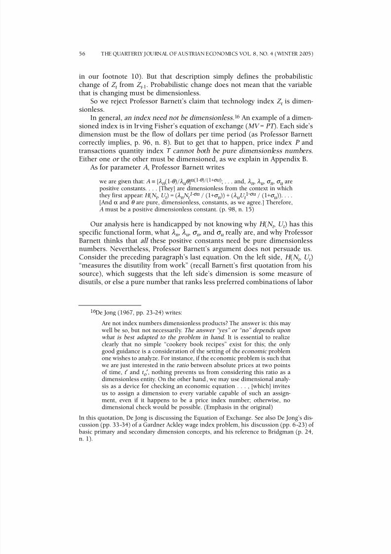
in our footnote 10). But that description simply defines the probabilisticchange of Z t from Z t -1. Probabilistic change does not mean that the variablethat is changing must be dimensionless.

So we reject Professor Barnett’s claim that technology index Z t is dimen-sionless.

In general, an index need not be dimensionless .16 An example of a dimen-sioned index is in Irving Fisher’s equation of exchange (MV = PT ). Each side’sdimension must be the flow of dollars per time period (as Professor Barnettcorrectly implies, p. 96, n. 8). But to get that to happen, price index P andtransactions quantity index T cannot both be pure dimensionless numbers .Either one or the other must be dimensioned, as we explain in Appendix B.

As for parameter A , Professor Barnett writes

we are given that: A ≡ [λ n(1-θ )/λ uθ ]α(1-θ )/(1+σ u); . . . and, λ n, λ u, σ n, σ u are

positive constants. . . . [They] are dimensionless from the context in which

they first appear: H (N t , U t ) = (λ nN t 1- σ n / (1+σ n)) + (λ uU t 1 -σ u / (1+σ u)). . . .[And α and θ are pure, dimensionless, constants, as we agree.] Therefore,A must be a positive dimensionless constant. (p. 98, n. 15)

Our analysis here is handicapped by not knowing why H (N t , U t ) has thisspecific functional form, what λ n, λ u, σ n, and σ u really are, and why ProfessorBarnett thinks that all these positive constants need be pure dimensionlessnumbers. Nevertheless, Professor Barnett’s argument does not persuade us.Consider the preceding paragraph’s last equation. On the left side, H (N t , U t )“measures the disutility from work” (recall Barnett’s first quotation from hissource), which suggests that the left side’s dimension is some measure of disutils, or else a pure number that ranks less preferred combinations of labor



hours and effort—which Barnett (2003, pp. 42, 46, 48–55) might prefer to“disutils.” On the right side, the only symbols that Barnett does not claim tobe dimensionless are N t and U t , which respectively have dimension units of

labor-hours and labor-effort per elapsed time period. So something else on theright side—perhaps λ n and λ u—must have dimensions that “convert” labor-hours and labor-effort per elapsed time period into either disutils or a purenumber. If so, A cannot be dimensionless.

Given the available information, we see no reason to abandon our dimen-sions for Z t given in our (2a) and (2b), or our dimensions for A given in our(3a) and (3b). We see no dimensional problems in the macroeconomic modeldiscussed by Professor Barnett.

FINAL THOUGHTS

Economists may not pay much attention to dimensional analysis, but thatdoes not mean that unstated but implied dimensions and units are wrong orinvalid. To us, Professor Barnett has not demonstrated his specific allegationsof dimensional errors. And he has not persuasively shown any serious prob-lem—much less a fatal flaw—in contemporary mathematical economics,caused by dimensional errors .

But our critique of Barnett’s diagnosis does not imply that we judge themathematical economics patient to be healthy. In contemporary mainstreameconomics, there is plenty of misuse and abuse of mathematics that has noth-ing to do with dimensional errors: a propensity to disregard fundamental ele-ments of economic reality simply because they cannot be encapsulated inmathematical models; the misuse of mathematics to foster the illusion that

economists can provide decision makers with information that no individualmind can possess; and disguising normative judgments as being positive con-clusions of so-called welfare economic analysis (Boettke 1997 and Rothbard1956).

We do not share, however, the implacable hostility of some Misesians tothe use of mathematics in economics. Some economists find that mathemat-ics gets in the way of their thinking, in which case they shouldn’t use mathe-matics in their thinking process. Other economists find that mathematicshelps them to see variables and effects that they may otherwise overlook; tobetter distinguish endogenous from exogenous variables;17 and to avoiddeductive errors.18 After clarifying their thoughts, sometimes they can follow


17It is easy to go astray in verbal-logical analysis by improperly treating as exogenous,a variable that is endogenous: for example, implicitly treating (real) income as an exoge-nous variable while deriving the labor supply response to a wage change. See Gonzalez(2000).

18Those same economists can, of course, find mathematics not useful for thinkingabout some issues, despite finding it useful for other issues.



Alfred Marshall’s famous advice to “Burn the mathematics.”19 But on otheroccasions they should publish rather than burn the mathematics: a lot of obscurity, misinterpretation, and semantic debates can be avoided by com-

municating some ideas with the assistance of some mathematics.Moreover, economics is more than economic theory. Most economists

want to address issues that require going beyond economic theory. Since eco-nomic theory’s laws always are qualitative, never quantitative, no reasonableestimate or even educated guess can be made about the magnitude of any eco-nomic effect, unless one is willing to go beyond the realm of pure economictheory. With theory alone, for example, one cannot assess the employmenteffect of a twenty percent hike in the Federal minimum wage. In fact, and con-trary to what some economists incorrectly believe, one cannot derive even thesign of the employment effect from only the pure Misesian logic of choice.20

Specific economic functions simply are tools of historical analysis. Theirusefulness in applied economics cannot be decided a priori ; it must be judgedby how well they perform their intended use.

The extent to which mathematics can assist the Austrian research pro-gram is an empirical issue. But there is no reason for Austrians to fear math-ematics properly used. The rejection of mathematics is neither necessary norsufficient for doing good economics. And the use of mathematics is neithersufficient nor necessary for doing bad economics. What distinguishes Aus-trian economics from bad economics is the Austrian theoretical hardcore.


19In 1906, Alfred Marshall wrote:

I had a growing feeling in the later years of my work at the subject thata good mathematical theorem dealing with economic hypotheses was very unlikely to be good economics: and I went more and more on therules—(1) Use mathematics as a shorthand language, rather than as anengine of inquiry. (2) Keep to them until you have done. (3) Translateinto English. (4) Then illustrate by examples that are important in reallife. (5) Burn the mathematics. (6) If you can’t succeed in (4), burn (3).

This last I did often.Favorably quoted by many economists, for example by Colander (2001, p. 131), citing thefollowing source: “From a letter from Marshall to A.L. Bowley, reprinted in A.C. Pigou,Memorials of Alfred Marshall, p. 427.”

20The Misesian logic of choice tells us that employers will not willingly hire labor whose marginal hiring cost exceeds its marginal benefit. It does not tell us, however, whatcounts as a hiring cost and what counts as a hiring benefit in employers’ minds, or whether the affected labor markets are competitive or monopsonistic.



A PPENDIX A THE COBB -DOUGLAS PRODUCTION FUNCTION’S LIMITATIONS

In its traditional form, the Cobb-Douglas production function is written Q =AK α Lβ , where Q is output, and K and L are real capital and labor inputs,respectively. It can also be written more generally, for one output q producedby I inputs x i , as:21

q = f (x 1, x 2 , x 3 , . . . x i , . . . x I ) = ax 1α

1x 2

α 2 x 3

α 3 . . . x i

α i . . . x I

α I

But in either its traditional or more general form, this specific multiplicativeproduction function has several seriously unrealistic characteristics.

(a) Because it is multiplicative, if any input quantity is zero, output quantity

is zero, no matter how many other nonzero input variables there are, orhow large their quantities are. Every input is essential.

(b) Because it has only one term, it cannot exhibit positive followed by nega-tive returns—if using more of a single input initially increases output quan-tity, using much more of that input cannot decrease output quantity: in aCobb-Douglas world, excess fertilizer never could burn plants enough todecrease corn output.22

(c) Because it is multiplicative with only one term, returns to a single variableinput (holding all other inputs constant) cannot change; they always willbe qualitatively the same. In a Cobb-Douglas production function,


21In a Cobb-Douglas type (single-term multiplicative) production function, the initialcoefficient (A or a0 ) and the input exponents (α and β or α i ) usually are positive, so thatoutput increases as the i th input increases. However, if the production process must cope with production impediments (cotton production in a world containing boll weevils comesto mind), the impeding variable’s exponent would be negative.

For any single-output multiple-input production function, output quantity q and usu-ally all input quantities x i are defined as flows (for example, flows of raw materials andof labor and real capital services) per time period rather than as stocks at a point in time.But for inputs such as dirt in a production function for housing services or perhaps foragriculture, or catalyst inputs in an oil refinery, the appropriate input dimension could bean unchanging stock measured at a point in time.

22However, a Cobb-Douglas type production function can be generalized by adding asecond term:

q = f (x 1, x 2 , x 3 , . . . x i , . . . x I ) = a0 x 1α 01x 2

α 02 x 3 α 03 . . . x i

α 0i . . . x I α 0I +

a1x 1α 11x 2

α 12 x 3 α 13 . . . x i

α 1i . . . x I α 1I

If a1 < 0, negative returns to single inputs become possible. This two-term multi-plicative function remains homogeneous of degree h (see our note 25), if h = Σα 0i = Σα 1i , where the summations are i = 1, 2 , 3 , . . . I .



increasing the variable input quantity always will increase output quantityat either an increasing, a constant, or a decreasing rate. As the one variableinput increases, output quantity never will switch from, say, increasing at

an increasing rate to increasing at a constant or decreasing rate, no matterhow small or large the single variable input quantity is.23 If diminishingreturns occur, they must occur not only eventually but also initially, assoon as the variable input quantity begins to increase from zero. (Differentinputs can, however, have qualitatively different returns: for example, if output increases at an increasing rate as input i increases, output mayincrease at a decreasing rate as a different input j increases—in each casechanging only one input quantity and holding all other inputs constant.)In more general production functions,24 “returns” to a single variable inputcan change: as a single variable input quantity increases, the rate at whichoutput increases can switch among increasing, constant, or decreasing.

And because the Cobb-Douglas function is homogeneous,25 it cannot haveinflection points at which the relationship between output quantity and twoor more input quantities can switch among convex, linear, or concave, and itcan have no freestanding additive constant. (The “homogeneity” name comes


23For any production function, whether a single variable input increases output at anincreasing, constant, or decreasing rate is determined by the sign (positive, zero, or nega-tive) of the function’s second partial derivative with respect to that input. But for a multi-plicative function, returns to a single input cannot vary qualitatively, because the sign of the second partial derivative with respect to an input will always be either positive, zero,or negative (depending on whether the input’s exponent parameter’s sign is greater than,equal to, or less than 1), regardless of the variable input’s quantity. [The statement inparentheses assumes f (⋅) > 0.]

24Including some homogeneous production functions. (For homogeneity, see our nextnote). For specific examples, see the string of thirteen American Economic Review Com-munications on “Diminishing Returns and Linear Homogeneity,” from Nutter (1963) toPiron (1966) and Eichhorn (1968). For the complete list, see their references. Also relevantis Levenson and Solon (1966).

25To define homogeneity, first consider a general (not necessarily homogeneous)function q = f (x 1, x2, x 3 , . . . x i , . . . x I ), with q o = f (x 1o , x 2o , x 3o , . . . x io , . . . x Io ) forany set of specific x i = x io values. This function is homogeneous of degree h if and onlyif multiplying all x io values by η gives q = ηhq o = ηhf (x 1o , x 2o , x 3o , . . . x io , . . . x Io ) =f (ηx 1o , ηx 2o , ηx 3o , . . . ηx io , . . . ηx Io ). That is, a function is homogeneous of degree h if and only if ηh can be “factored completely out” of the entire function, when within thefunction each independent variable is multiplied by η. Any Cobb-Douglas type (single-term multiplicative) function always satisfies this condition, with h = α + β or h = Σα i .

In contrast, a polynomial function is homogeneous of degree h only in the specialcase that in every term, its variables’ exponents sum to h. To convert an ordinary polyno-mial to homogeneity of degree h, the coefficients of all terms whose variables’ exponentsdo not sum to h must be set to zero (which, assuming h > 0, includes setting the additiveconstant term to zero). Homogeneity is very restrictive. An ordinary polynomial, no termsforced to zero, third degree (cubic) or higher to allow inf lections between convex and con-cave, usually is a much more realistic theoretical representation of almost any productionrelationship.



from these “same shape” characteristics.) All homogeneous functions have thefollowing “returns to scale” properties:

(d) Holding only some (or no) input quantities constant, with an initial mixof at least two variable inputs, returns to scale for that mix of variableinputs cannot change: increasing all variable input quantities together (infixed proportions) always will increase output quantity at either anincreasing, a constant, or a decreasing rate. As the variable inputs increase(“scale up”) together, output quantity never will switch from, say, increas-ing at an increasing rate to increasing at a constant or decreasing rate. Fora given set of constant inputs, returns to scale for the variable inputsalways will be qualitatively the same, no matter how small or large thefixed-proportion package of variable inputs is.26

(e) Again holding only some (or no) input quantities constant, changing the

initial mix of the variable inputs does not change whether scaling up allof the variable input quantities increases output at an increasing, con-stant, or decreasing rate. That is, for a given set of constant inputs, returnsto scale always will be qualitatively the same—increasing, constant, or decreasing—no matter what mix of variable inputs is “scaled up” in fixedproportions.27


26For any production function, to determine its returns to scale, first replace each of its fixed inputs x i by x i

# (the superscript # denotes a constant value variable), and replaceeach of its variable inputs x j that will change only in fixed proportion by ηx jo , where η is

the “scale factor” that will determine how much of the initial mix of variable inputs willbe used. Then the sign of function’s second partial derivative with respect to η (holdingthe x i

# and x jo constant) will give the function’s returns to scale, which in general may vary among increasing, constant , or decreasing, as η increases. But in any homogeneousfunction, including the Cobb-Douglas function, this second derivative’s sign is constant(either positive, zero, or negative), not affected by the magnitude of η.

Geometrically, consider a three-dimensional two-variable-input production functionin the corner of a room. Input space is on the floor. The horizontal x 1 and x 2 input axeseach are where the f loor meets a wall. The vertical q output quantity axis is where the two walls intersect. In input-space on the f loor, the origin at the corner of the room, together with the point defined by x 1o and x 2o , define a ray. Changes in the value of scale factor ηmove along that ray. Above that ray, in output space, is the output quantity q generated bydifferent values of η. As η increases, output increases at either an increasing, constant, ordecreasing rate of return to scale. But if the function is homogeneous, the rate of return

to scale never switches from one curvature to another.27To demonstrate this property for any homogeneous function, including the Cobb-

Douglas function, note from the preceding note’s calculations that the sign of the secondpartial derivative of the function with respect to η is not affected by changes in any of the variable input quantities x jo [assuming f (⋅) remains f (⋅) > 0]. Geometrically, in the preced-ing note’s three-dimensional room-corner diagram (of a homogeneous production func-tion), above any ray on the floor, as η increases, output always increases at either anincreasing, constant, or decreasing rate of return to scale, regardless of the ray considered.



(f) And a homogeneous function (of degree h > 0) can have no additive con-stant term, although such a term (if positive) allows for some minimumoutput quantity to be provided by nature, or (if negative, together with a

nonnegativity condition for the function’s output quantity) allows inputquantities to reach some minimum before any output is produced.

Professor Barnett’s “Dimensions and Economics” paper (2004) does notdeal with any of these limitations.28 He focuses his attention on variable andparameter dimensions (pp. 95, 96–98).29

A PPENDIX BFISHER ’S EQUATION OF EXCHANGE, A DIMENSION FOR EITHER P OR T

In Irving Fisher’s equation of exchange (MV = PT ), the left side is the dollar value of the flow of spending per time period; the right side is the dollar value

of the flow of transaction receipts per time period [what might be called nom-inal “Gross Gross Domestic (or National) Product,” since Fisher’s equationincludes intermediate transactions among businesses (and, by extension,among businesses and governments and between both)]. The economy’s grossspending equals its gross receipts, in dollars (or any other monetary unit).The dimension units on both sides—dollars/time-period—must match.


28In an earlier paper, Professor Barnett (2003) does point out two of the above Cobb-Douglas function characteristics: (a) for production functions and (d) for utility functions(p. 47, notes 12 and 13 respectively).But we disagree with his claim (note 13) that for a

utility function, “a scale increase of the arguments [that] gives rise to a greater scaleincrease in utility . . . [does not accord] with human action.” That statement refers to car-dinal (vice ordinal) values. It is true (as Barnett says) that any particular utility function’sdependent variable values, independent variable values, and the results that describe con-sumer choice actions, all are cardinal . But those cardinal results (behavior and demandfunction descriptions) depend only on the utility function values’ ordinal property (larger values represent preferred bundles). For successively preferred bundles, successive incre-ments of larger utility values are arbitrary—they can be of any positive size. Thus any increasing monotonic transformation of a utility function has no effect on the function’sresults that describe consumer choices: its first finite difference quotient (in the limit,derivative) with respect to scale must be positive, but its second and higher finite differ-ence quotients (or derivatives) can be of any sign. (Derivatives, of course, require conti-nuity, a simplifying but often suspect assumption, as Barnett argues on pages 57–59.)

29Professor Barnett does say (2004, p. 95, n. 5), that because a function’s dependent variable must be unique for any set of independent variable values, “it is incorrect toexpress any production relationships [as functions?] in any case in which Leibensteinianstyle X-inefficiency can exist.” (See also the macroeconomic model on his page 97, includ-ing note 12.) We would rather say that the traditional production function describes themaximum output quantity—not the feasible set of output quantities—that the firm canobtain from a given set of input quantities. Given such a production function, to describenot the maximum output quantity but instead the feasible set of output quantities, convertthe production function equation into a relation, by replacing the = sign by a ≤ sign.



On the left side, M is the money stock at a point in time; V is the turnoverof that money stock per time interval (e.g. 30 per year); MV is the stock of dol-lars times 30/year, which is the f low of dollars spent per year. (After stripping

out the magnitudes of these variables, M ’s dimension unit is simply dollars;V ’s dimension unit is 1/year.) So far, no problem.

On the right side, things are not quite that simple. It is tempting to defineprice index P as a dimensionless (pure) number ratio of the sums of (quan-tity weighted) prices for two time periods, and transactions quantity index T as a dimensionless (pure) number ratio of the sums of (price weighted) trans-action quantities for two time periods. But if we do that, then multiplying thetwo dimensionless numbers P and T gives another dimensionless number,rather than a flow of gross receipts of dollars per year.

Therefore, in the equation of exchange, price index P as a dimensionlesspure number ratio and transactions quantity index T as a dimensionless purenumber ratio, cannot hold simultaneously . The solution is that either one or

the other ratio must be multiplied by the flow of nominal transaction quanti-ties during the base time period, thus making either P or T a dimensionedindex.30

That conclusion applies not only to Fisher’s equation, but also to a “nom-inal income” equation of exchange (MV = PQ ), in which the right side doesnot include intermediate transactions but instead is nominal Gross Domestic(or National) product [Q or sometimes Y being real Gross Domestic (orNational) product], and Velocity is a substantially smaller number than inFisher’s equation.

A more detailed and more symbolic version of this argument31 follows.Let ∆t be the length of a time period, in whatever units time is measured:

if time is measured in years with 52 weeks per year, then a thirteen week time


30Barnett (2004, pp. 100, 101) mentions that a referee for “a leading English-languageeconomics journal” wrote Barnett that

Dimensional analysis can only be applied to laws . . . . Fisher’s relation of exchange . . . MV = PT . . . is one of the few examples that comes closestto a law. One result of dimensional analysis is that there is somethingodd with this equation. The left part does contain a time dimension, while the right side doesn’t. This is not something new and can be foundin any textbook.

We see no reason for dimensional analysis to be limited to “laws,” and we wonder howthe referee would define them, and we’d like to see a representative “any textbook,” butthat’s not why we have quoted that referee.

Instead, we suggest that not seeing the right side’s time dimension may result fromassuming that P and T both are dimensionless pure ratios. The right side’s time dimen-sion comes from multiplying either the price or transaction ratio by the flow of nominaltransaction quantities during the base period.

31Based on Boulding (1966, pp. 27–28); and loosely on De Jong (1967, pp. 23–30).



period is ∆t = 0.25 years. A time interval equals or is some multiple of the timeperiod ∆t .

On Fisher’s left side, M is the money stock at a point in time (at a time

interval’s end; a more general formulation would allow the point in time to beanywhere in the interval), with its dimension units simply being dollars.

Velocity is the money stock’s average turnover per time period (during theinterval), so it is a number (say 20 times per year, or 5 times per quarter), withdimension units 1/period. Multiplying M by V gives left side dimension unitsof dollars/time period.

On Fisher’s right side, P is a price index, and T is a transactions quantityindex. Let p j and q j represent the price and quantity of the j th transaction, andsuperscripts b and e respectively represent the base period and end period

within the interval. Assume P is a Laspeyres index (base period quantity weights). Then the end period dollar value of the f low of transaction receipts

per time period is: PT = Σ p j e

q j e

, whereP = Σ p j e q j b / Σ p j b q j b , andT = [Σ p j e q j e / Σ p j e q j b ]⋅Σ p j b q j b .

The transactions index T , rather than being a pure ratio, has been rede-fined into a dimensioned index.

Alternatively, the Laspeyres price index P could be redefined into a dimen-sioned index as P = [Σ p j e q j b / Σ p j b q j b ]⋅Σ p j b q j b = Σ p j e q j b , so that T would be apure ratio.

Analogous results hold if P is a Paasche price index (end period quantity weights), and T is defined accordingly (the final factor of either T or P againis Σ p j b q j b ).

R EFERENCES

Barnett II, William. 2004. “Dimensions and Economics: Some Problems.” Quarterly Jour- nal of Austrian Economics 7 (1): 95–104. An earlier version of the article appeared inthe Quarterly Journal of Austrian Economics 6 (3): 27–46. It was reprinted in 2004 tocorrect formatting and typographical errors.

———. 2003. “The Modern Theory of Consumer Behavior: Ordinal or Cardinal?” Quarterly Journal of Austrian Economics 6 (1): 41–65.

Baumol, William. 1977. Economic Theory and Operations Analysis . 4th ed. EnglewoodCliffs, N.J.: Prentice-Hall.

Blaug, Mark. 1998. “Disturbing Currents in Modern Economics.” Challenge, The Maga-

zine of Economic Affairs 41, no. 3 (May–June): 11–34. Includes numerous referencesto other mainstream economists’ objections to “soporific scholasticism” and the math-ematizing of contemporary economics.

Boettke, Peter J. 1997. “Where Did Economics Go Wrong? Modern Economics as a Flightfrom Reality.” Critical Review 11 (1): 11–64.

Boulding, Kenneth E. 1966. Economic Analysis . Vol. II: Macroeconomics . 4th ed. New York: Harper and Row, Publishers.




Colander, David C. 2001. Economics . 4th ed. Boston: McGraw-Hill Irwin.

Courant, Richard, and Herbert Robbins. [1941] 1969. What Is Mathematics? London:Oxford University Press.

De Jong, Frits J., and Wilhelm Quade. 1967. Dimensional Analysis for Economists. With aMathematical Appendix on the Algebraic Structure of Dimensional Analysis . Amster-dam: North-Holland Publishing.

Eichhorn, Wolfgang. 1968. “Diminishing Returns and Linear Homogeneity: Final Com-ment.” American Economic Review 58 (1): 150–62.

Gonzalez, Rodolfo A. 2000. “Misesian Economics and the Response to a Price Change.”Quarterly Journal of Austrian Economics 3 (1): 55–58.

Hazlitt, Henry. 1959. The Failure of the “New Economics.” Princeton, N.J.: D. Van Nos-trand.

James, Robert C., and Edwin F. Beckenbach. 1968. James & James Mathematics Dictio- nary . Third Edition. Original and First editions inspired by Glenn James. Additionalcontributions by Armen A. Alchian, Clifford Bell, Homer V. Craig, Aristotle D. Michal,and Ivan S. Sokolnikoff. New York: Van Nostrand Reinhold.

Leoni, Bruno, and Eugenio Frola. [1955] 1977. “On Mathematical Thinking in Economics.” Journal of Libertarian Studies 1 (2): 101–09. In slightly altered form, originally deliv-ered at the Center of Methodological Studies at Turin, and published in Italian, in Il Politico (Anno XX, no. 2). Later delivered at the School of Economics at the Univer-sity of Manchester.

Levenson, A.M., and Babette Solon. 1966. “Returns to Scale and the Spacing of Iso-quants.” American Economic Review 61 (3): 501–05.

Mises, Ludwig von. [1953] 1977. “Comments About The Mathematical Treatment of Eco-nomic Problems.” Journal of Libertarian Studies 1 (2): 97–100. Translated by HelenaRatzka, from “Bemerkungen über die mathematische Behandlung nationalökonomis-cher Probleme.” Studium Generale VI, no. 2.

———. 1966. Human Action. 3rd rev. ed. Chicago: Henry Regnery.

Nutter, G. Warren. 1963. “Diminishing Returns and Linear Homogeneity.” American Eco- nomic Review 53 (5): 1084–85.

Pigou, Arthur Cecil, ed. [1925] 1966. Memorials of Alfred Marshall . Reprinted at New York: Augustus M. Kelley.

Piron, Robert. 1966. “Diminishing Returns and Linear Homogeneity: Further Com-ment.” American Economic Review 56 (1): 183–86.

Rothbard, Murray N. 1956. “Toward a Reconstruction of Utility and Welfare Economics.”In On Freedom and Free Enterprise . Mary Sennholz, ed. Princeton, N.J.: D. Van Nos-trand.


Documents

Dimensional Analysis in Economics