Dilute gas of ultracold two-level atoms inside a cavity: generalized Dicke model

This article has been downloaded from IOPscience. Please scroll down to see the full text article.

2009 New J. Phys. 11 063027

(http://iopscience.iop.org/1367-2630/11/6/063027)

Download details:

IP Address: 147.83.123.136

The article was downloaded on 22/06/2009 at 09:41

Please note that terms and conditions apply.

The Table of Contents and more related content is available

HOME | SEARCH | PACS & MSC | JOURNALS | ABOUT | CONTACT US

T h e o p e n – a c c e s s j o u r n a l f o r p h y s i c s

New Journal of Physics

Dilute gas of ultracold two-level atoms insidea cavity: generalized Dicke model

Jonas Larson1,4 and Maciej Lewenstein2,3

1 NORDITA, 106 91 Stockholm, Sweden2 ICFO—Institut de Ciències Fotòniques, E-08860 Castelldefels (Barcelona),Spain3 ICREA—Institució Catalana de Recerca i Estudis Avançats,E-08010 Barcelona, SpainE-mail: jolarson@kth.se

New Journal of Physics 11 (2009) 063027 (18pp)Received 26 February 2009Published 16 June 2009Online at http://www.njp.org/doi:10.1088/1367-2630/11/6/063027

Abstract. We consider a gas of ultracold two-level atoms confined in a cavity,taking account of atomic center-of-mass motion and cavity-mode variations. Weuse the generalized Dicke model (DM), and analyze separately the cases of aGaussian, and a standing wave mode shape. Owing to the interplay betweenexternal motional energies of the atoms and internal atomic and field energies,the phase-diagrams exhibit novel features not encountered in the standard DM,such as the existence of first- and second-order phase transitions between normaland superradiant phases. Due to the quantum description of atomic motion,internal and external atomic degrees of freedom are highly correlated leadingto modified normal and superradiant phases.

4 Author to whom any correspondence should be addressed.

New Journal of Physics 11 (2009) 0630271367-2630/09/063027+18$30.00 © IOP Publishing Ltd and Deutsche Physikalische Gesellschaft

2

Contents

1. Introduction 22. Generalized DM and its partition function 43. Transversal thermodynamics 5

3.1. Derivation of the partition function for transversal motion . . . . . . . . . . . . 53.2. Numerical results . . . . . . . . . . . . . . . . . . . . . . . . . . . . . . . . . 73.3. Validity of the adiabatic approximation . . . . . . . . . . . . . . . . . . . . . . 11

4. Longitudinal thermodynamics 125. Conclusions 14Acknowledgments 14Appendix. Tight-binding approach 14References 16

1. Introduction

Progress in trapping and cooling of atomic gases [1] has made it possible to coherently couplea Bose–Einstein condensate to a single cavity mode [2]. These experiments pave the way toa new subfield of AMO physics; many-body cavity quantum electrodynamics. In the ultracoldregime, light-induced mechanical effects on matter waves lead to intrinsic nonlinearity betweenthe matter and the cavity field [3, 4]. In particular, the nonlinearity renders novel quantumphase transitions (QPT) [5]. Other related QPTs in cavity QED models have been presentedin [6]. Such nonlinearity, due to the quantized motion of the atoms, is absent in the so-calledstandard Dicke model (DM). Explicitly, the DM describes a gas of N non-moving two-levelatoms interacting with a single-quantized cavity mode [7]. The interplay between the fieldintensity/energy, the free atom energy, and the interaction energy leads to a quantum phasetransition (DQPT) in the DM. Motivated by the novel phenomena arising from a quantizedtreatment of atomic motion [4, 8], it is highly interesting to extend the DM to include atomicmotion on a quantum scale, and in particular to analyze how it affects the nature of the DQPT.It is clear that such generalization of the DM results in new aspects of the system properties.The atomic motion is directly affected by the shape of the field induced potentials, which inreturn is determined by the system parameters and the field intensity. In addition to the termscontributing to the total energy in the regular DM, in this model we have to take into accountthe motional energy of the atoms. This enters in a nontrivial way since the interaction energydepends on the motional states of the atoms.

The DM was first introduced in quantum optics to describe the full collective dynamics ofatoms in a high-quality cavity. The DM Hamiltonian, given in the rotating wave approximation(RWA), reads

HD = hωa†a +h

2

N∑i=1

σ zi +

hλ√

N

N∑i=1

(a†σ−

i + σ +i a). (1)

Here, the boson ladder operators a† and a create and annihilate a photon of the cavity mode, thePauli σi -operators act on atom i , ω, and λ are the mode and atomic transition frequenciesand effective atom–field coupling, respectively. The DM is a well-defined mathematical

New Journal of Physics 11 (2009) 063027 (http://www.njp.org/)

3

model for any value of its parameters. Note, however, that whether this model describesfaithfully some physical situation for any choice of parameters is not guaranteed. Formoderate λ, the DM appropriately describes the dynamics of atoms coupled to the cavityfield, and it has been thoroughly discussed in terms of collapse-revivals [9], squeezing [10],entanglement [11] and state preparation [12]. Considerable interest, however, has been devotedto the normal–superradiant phase transition [13]–[15].

In the thermodynamic limit (N , V → ∞, N/V = const) the system exhibits a nonzerotemperature phase transition between the normal phase and the superradiant phase. Inthe normal phase, all atoms are in their ground state and the field in vacuum, whereas thesuperradiant phase is characterized by a nonzero field and a macroscopic excitation of thematter. Its critical coupling and critical temperature are [13]

λc =√

ω,

(kBTc)−1

=2ω

arctanh

(ω

λ2

).

(2)

As was shown in [14], the critical coupling can be seen as a condition on the atomic densityρ = N/V . Interestingly, the DQPT is of second-order nature without the RWA, whereas it is firstorder if the RWA has been imposed [16]. The corrections due to the RWA to various physicalobservables have been considered [15, 17].

More detailed analysis of miscellaneous aspects of the DQPT have been presented innumerous publications. In particular, various extensions [18, 19] as well as approximatemethods [20] concerning the DQPT have been outlined. Recently, Emary and Brandes appliedthe algebraic Holstein–Primakoff boson representation to the DM. The method turned out to bevery powerful and has since then been applied frequently to the DM [21].

Despite the numerous publications on the DQPT, the existence of this phase transition hasbeen widely discussed. If the two-level atoms in the DM correspond to atoms in a ground andexcited state, and the transition is direct, then quantum mechanics forbids the transition. This canbe seen either by realizing the necessity of adding the, so-called, A2-term to the Hamiltonian,or by employing sum rules to bound the coefficients in the DM to the ‘trivial’ thermodynamicalphase [24]. The argumentation of [24] can be generalized to a quite general no-go theorem forthe DQPT [25], but it does not apply if the two-level atoms in the DM correspond to atoms intwo excited states, such as Rydberg states, or if the transition is not direct.

One valuable step towards an experimental realization of the DQPT was taken in relationwith [22], where typical experimental parameters as well as losses were included. These authorsconsidered the two levels coupled by a non-resonant Raman transition. In such conditions, theatom–field coupling λ can be tuned more or less independently of the A2 term in an effectivetwo-level model, and one can reach the regime of DQPT. This paper, however, considers asituation in which atomic motion can be neglected due to high temperatures, e.g. the standardDQPT. An alternative situation, in which the atomic motion could be neglected, would be toconsider quantum dots interacting with a cavity mode [19, 23].

In this paper, we extend the DM to take into account atomic motion in a fully quantummechanical description. The atomic motion then introduces an additional degree of freedom tothe problem, leading to novel appearances of the system phase diagrams. The gas is assumeddilute such that atom–atom scattering can be neglected, and that the motion is restrictedto one dimension due to tight confinement in the remaining two directions via external

New Journal of Physics 11 (2009) 063027 (http://www.njp.org/)

4

trapping. Furthermore, the atoms are assumed trapped by the cavity field itself. Consequently,a normal–superradiant QPT is not possible, since for a vanishing field the atomic trappingcapability is lost. However, we may assume a lowest bound of the field such that at leastone bound state of the trapping ‘potential’ is guaranteed. This can be achieved by an externalpumping of the cavity, which imposes a non-vanishing cavity field. Our research is partlycarried out in the adiabatic regime, motivated by the ultracold atoms considered and itsjustification is numerically verified. In this adiabatic regime, the problem relaxes to solving aone-dimensional (1D) time-independent Schrödinger equation. In particular, we study the caseof a Gaussian mode profile utilizing this adiabatic method. The situation with a standing wavemode profile is also considered, however using a full numerical rather than adiabatic approach.For a Gaussian profile the number of bound states is crucial for the thermodynamics, and wefind great divergences from the regular DM. Among these are the existence of both first- andsecond-order QPTs and multiple superradiant phases. The second, standing wave mode, showsslight similarities to the model of [19] but the QPT is found to be of second order, and the PTsurvives for zero temperature and finite ω opposite to the regular DQPT.

The paper is organized as follows. In the next section, we present the generalized DMthat includes the motion of the atom. The adiabatic diagonalization of the single particleHamiltonians utilized for the Gaussian mode profile is introduced and the general expressionfor the partition function given. The following section 3 considers the situation of a Gaussianmode profile. We thoroughly discuss the importance of bound states. Section 4 instead considersa standing wave mode profile in a fully numerical fashion. In the appendix, however, we deriveanalytical expressions in the regimes of tight binding, which provides us with various asymptoticproperties. Finally we conclude with a summery in section 5.

2. Generalized DM and its partition function

We consider a gas of N ultracold identical two-level atoms, with mass m and energy levelseparation h, interacting with a single cavity mode with frequency ω. For a low-temperaturegas, we include atomic center-of-mass motion and mode variation. In the RWA and dipoleapproximation, the extended DM becomes

H = ωa†a +N∑

i=1

[p2

i

2+

2σ z

i +g(xi)√

V

(a†σ−

i + σ +i a)]

. (3)

Here, pi and xi are the scaled center-of-mass momentum and position of atom i , respectively,g(x) the effective position-dependent atom–field coupling and V the mode volume. Throughoutthe paper we will use scaled variables such that h = m = 1. The case of a single atom is givenby the generalized Jaynes–Cummings Hamiltonian studied by numerous authors [26, 28].

In the thermodynamic limit, we let V → ∞ and N → ∞ such that the atomic density isfixed; ρ = N/V ≡ ρ0. The partition function reads

Z = Tr[e−β H

], (4)

where β−1= T and T is the scaled temperature and the trace is over the field and atomic degrees

of freedom. It is convenient to perform the trace of the field in terms of Glauber’s coherent states,a|α〉 = α|α〉. In the thermodynamic limit, one may replace a → α and a†

→ α∗ in the evaluationof the partition function [13]. In other words; in the large atom number limit the photon

New Journal of Physics 11 (2009) 063027 (http://www.njp.org/)

5

ladder operators, or more precisely a/√

N and a†/√

N , can be treated as commuting operators.Using the fact that atomic operators mutually commute between themselves, for example[xi , p j ] = iδi j , the partition function can be written

Z =

∫d2α

πe−βω|α|

2

Tr[e−βh(α)

]N, (5)

where the integration is over the whole complex α-plane and

h(α) =p2

2+

2σ z +

g(x)√

ρ0√

N

(ασ + + α∗σ−

). (6)

In the sense of ultracold atoms as considered here, the kinetic energy of the atoms isassumed smaller than the effective potential energy. Provided that the adiabatic potentials do notcross, it is then legitimized to perform an adiabatic diagonalization of the internal states [27]. Inthis regime, the single particle Hamiltonian relaxes to two decoupled adiabatic ones

h±

ad(|α|) =p2

2+ V ±

ad (x, |α|2)

≡p2

2±

√2

4+

g2(x)ρ0

N|α|2. (7)

This approximation will be imposed in the next section considering a Gaussian mode profile.However, in the proceeding section dealing with the standing wave mode such an approachis not advocated, since then the curve crossings between the adiabatic potentials breakadiabaticity [27]. The justification of the adiabatic approximation applied to the Gaussian modeprofile will be discussed at the end of the next section. Within this regime, the problem hasbecome one of solving for the eigenvalues of two time-independent decoupled Schrödingerequations. The adiabatic Hamiltonians depend solely on the norm |α| and in polar coordinatesthe angle part can therefore be integrated out. By denoting the eigenvalues E±

n (r) respectively,where r = |α| and n is a quantum number/numbers that can be either discrete and/or continuous,we get the adiabatic partition function

Zad = 2∫

∞

0dr re−βωr2

Tr[e−βE+

n (r)]

+ Tr[e−βE−

n (r)]N

. (8)

Without loss of generality, we can choose ρ0 = 1 as it only scales the effective atom–fieldcoupling. It is worth mentioning that the numerics deal with exponentially large numbers,especially for small temperatures, which restrict the analysis to certain ranges.

3. Transversal thermodynamics

3.1. Derivation of the partition function for transversal motion

A Fabry–Perot cavity has eigenmodes that are, to a good approximation, Gaussian in thetransverse and harmonic in the longitudinal direction. Assuming an external deep trap in thelongitudinal direction and one transverse direction, we may consider the 1D problem in whichthe atom–field coupling has a spatial Gaussian shape. As is well known [26], and seen fromequation (7), only atoms in the ‘adiabatic’ internal state corresponding to the Hamiltonianh−

ad(r) will feel an attractive potential, whereas the others will be scattered away from the

New Journal of Physics 11 (2009) 063027 (http://www.njp.org/)

6

cavity field. We therefore consider only a sub ‘quasi’ Hilbert space containing the bound statesE−

n (r) of

h−

ad(r) =p2

2−

√2

4+

λ2r 2

Nexp

(−2

x2

12x

), (9)

where 1x is the transverse mode width.In order to proceed in an analytic way, we make the following approximate ansatz,√

2

4+

λr 2

Nexp

(−2

x2

12x

)≈ ε0 + U0 sech2(qx). (10)

The unknown constants are determined from the conditions: (i) the two functions have the sameasymptotic values for x → ±∞, (ii) their maximum are the same and (iii) they share the samefull-width at half-maximum (FWHM). Explicitly this yields

ε0 =

2,

U0(r2) =

√2

4+

λ2r 2

N−

2,

qr2 =

√2 arcsech

(√1/2

)1x

√√√√√√ln

4λ2r2

N

((√24 + λ2r2

N + 2

)2

−2

)

.

(11)

The bound eigenvalues of the Hamiltonian

h−

ad(r) =p2

2−

2− U0(r

2) sech2(qr2 x) (12)

are known to be [29]

E−

n (r 2) = −

2−

q2r2

8

[−(1 + 2n) +

√1 +

8U0(r 2)

q2r2

]2

. (13)

Let us introduce the number of bound states, for a given set of parameters, as N and define thefunction

g1(r2) =

N∑n=0

e−βE−n (r2). (14)

With this, the partition function (8), considering only bound states, becomes

Zad = 2∫

∞

0dr re−βωr2+N ln[g1(r2)]. (15)

By the variable substitution y = r 2/N we get

Zad = N∫

∞

0dy eN [−βωy+ln[g1(y)]]. (16)

New Journal of Physics 11 (2009) 063027 (http://www.njp.org/)

7

In the thermodynamic limit, this integral is solved by the saddle point method [30]

Zad = NC1√

Nmax

06y6∞

eN [−βωy+ln[g1(y)]]

, (17)

where C1 is a constant. Note that y has the meaning of scaled field intensity.One obstacle of the above model already mentioned in the introduction, is the fact that for

a shallow potential well the number of bound states will vanish. In this limit, the cavity field canno longer serve as a trap for the atoms. Consequently the ground state is the one of zero atoms,and we cannot have a proper thermodynamic limit N → ∞. We therefore add the constraintthat a minimum of one bound state is assumed. This can be met experimentally by including anexternal driving of the cavity mode, so that the field is nonzero throughout. Thus, the ‘normal’phase will contain a nonzero cavity field, which is sustained by the external pumping. We havenumerically checked that this does not introduce any significant changes in the analysis.

For the number N of bound states, we have

(1 + 2N ) <

√1 +

8U0(y)

q2y

. (18)

Naturally, N depends on the system parameters. As N is an integer, a change in thesystem parameters may bring about jumps between integer numbers of N . This will causediscontinuities in the function g1. Letting N = 1 we find U0(y) > q2

y . For small fields, y → 0,the potential amplitude U0 vanishes and the bound states cease to exist. However, for small butnonzero fields, the above inequality may be met for large couplings λ and widths 1x .

3.2. Numerical results

To study equation (17), we analyze the parameter dependence of the function

f1(y) = −βhωy + ln [g1(y)] . (19)

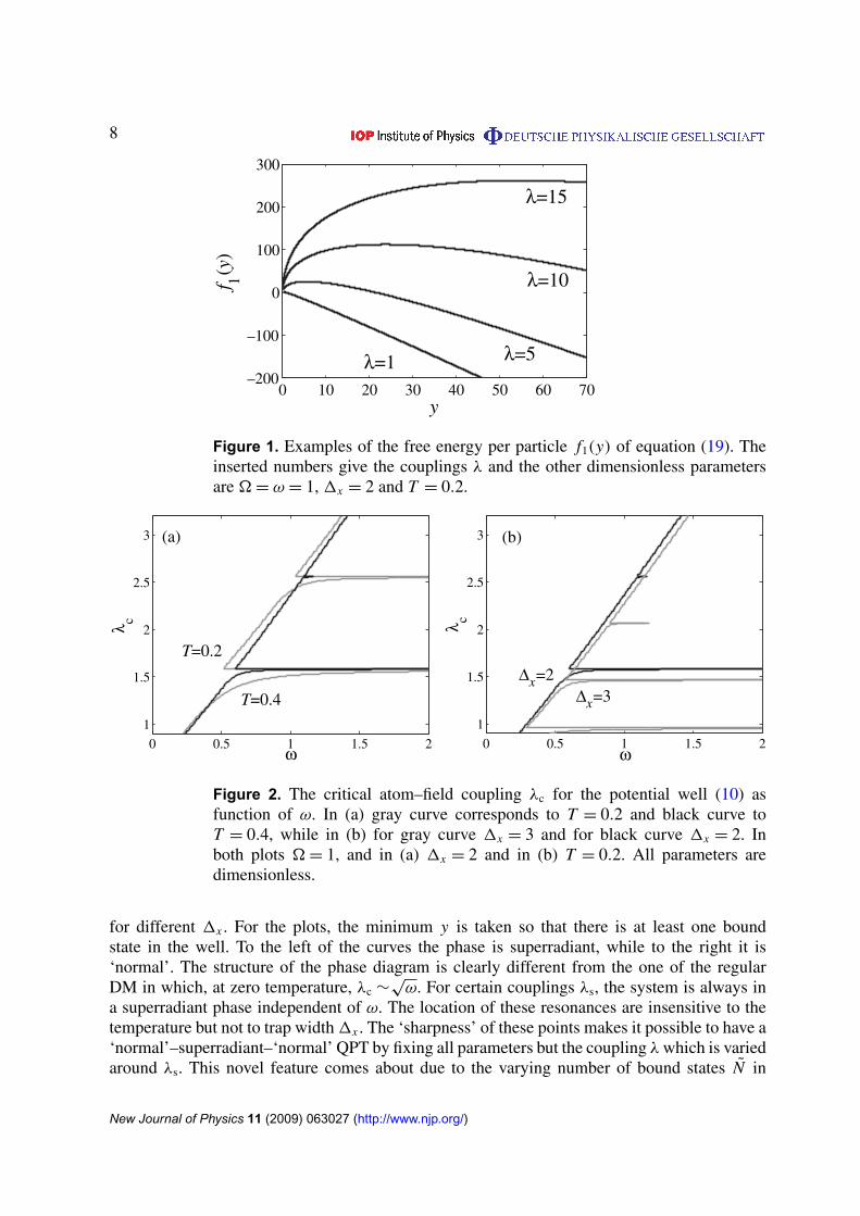
Note that f1(y) is the free energy per particle, given a scaled field intensity y. Let us brieflydiscuss characteristics of f1(y) before approaching it numerically. The first part arises from thebare field, and it is energetically favorable to have a vanishing field. The second part contains theatom–field interactions plus kinetic and potential atomic energies. The interaction energy entersindirectly into the atomic potential part. Increasing the field amplitude deepens the potential welland therefore lowers the energy, and it is therefore more beneficial to have a large field. The twoterms therefore compete, and in particular, the location of the maximum of f1(y) depends onthe particular system parameters used. Thus, atomic motion, directly related to the shape anddepth of the adiabatic potential, is a crucial ingredient for the QPT. If the smallest possibley maximizes the function, the system is said to be in a ‘normal’ phase (in quotes becausethe field is still nonzero to guarantee at least one bound state), while if a non-minimal y isoptimal the system is in a superradiant phase. In the limit of large y, the second term diverges asln[g1(y)] ∼

√y, whereas the first term goes as ∼−y, and we conclude that a maximum of f1(y)

is only obtained for a finite y. These reflections are numerically verified in figure 1 showingf1(y) for four different couplings λ. We see that there is a critical coupling λc: for λ < λc thesystem is in a ‘normal’ phase and for λ > λc it is in a superradiant phase.

In figure 2, we display the critical coupling λc as function of ω while keeping the otherparameters fixed. In (a) we present two examples for different T and in (b) two examples

New Journal of Physics 11 (2009) 063027 (http://www.njp.org/)

8

0 10 20 30 40 50 60 70–200

–100

0

100

200

300

y

f 1(y

)

λ=1 λ=5

λ=10

λ=15

Figure 1. Examples of the free energy per particle f1(y) of equation (19). Theinserted numbers give the couplings λ and the other dimensionless parametersare = ω = 1, 1x = 2 and T = 0.2.

1

1.5

2

2.5

3

0 0.5 1 1.5 2

λ c

ω

(a)

T=0.4

T=0.2

1

1.5

2

2.5

3

0 0.5 1 1.5 2

λ c

ω

(b)

∆x=3∆x=2

Figure 2. The critical atom–field coupling λc for the potential well (10) asfunction of ω. In (a) gray curve corresponds to T = 0.2 and black curve toT = 0.4, while in (b) for gray curve 1x = 3 and for black curve 1x = 2. Inboth plots = 1, and in (a) 1x = 2 and in (b) T = 0.2. All parameters aredimensionless.

for different 1x . For the plots, the minimum y is taken so that there is at least one boundstate in the well. To the left of the curves the phase is superradiant, while to the right it is‘normal’. The structure of the phase diagram is clearly different from the one of the regularDM in which, at zero temperature, λc ∼

√ω. For certain couplings λs, the system is always in

a superradiant phase independent of ω. The location of these resonances are insensitive to thetemperature but not to trap width 1x . The ‘sharpness’ of these points makes it possible to have a‘normal’–superradiant–‘normal’ QPT by fixing all parameters but the coupling λ which is variedaround λs. This novel feature comes about due to the varying number of bound states N in

New Journal of Physics 11 (2009) 063027 (http://www.njp.org/)

9

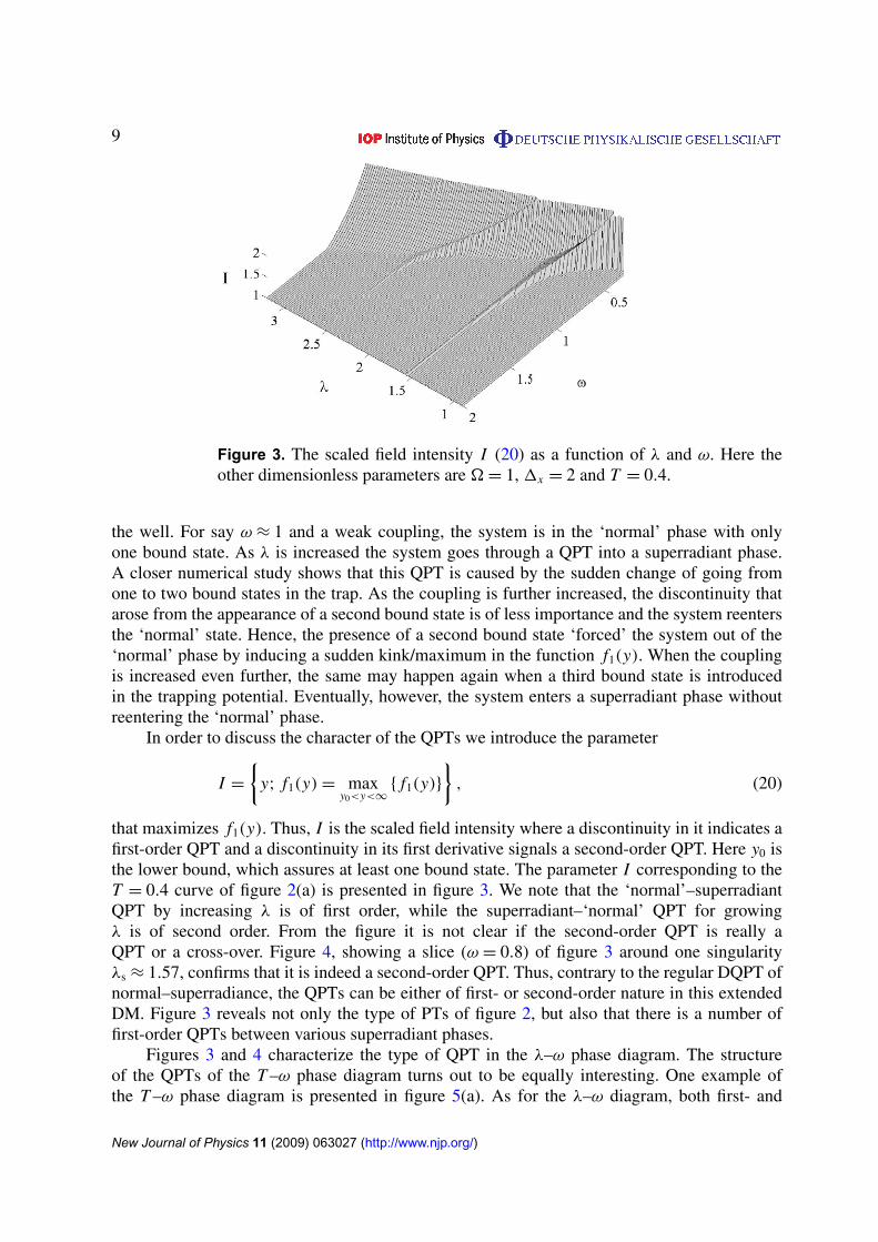
Figure 3. The scaled field intensity I (20) as a function of λ and ω. Here theother dimensionless parameters are = 1, 1x = 2 and T = 0.4.

the well. For say ω ≈ 1 and a weak coupling, the system is in the ‘normal’ phase with onlyone bound state. As λ is increased the system goes through a QPT into a superradiant phase.A closer numerical study shows that this QPT is caused by the sudden change of going fromone to two bound states in the trap. As the coupling is further increased, the discontinuity thatarose from the appearance of a second bound state is of less importance and the system reentersthe ‘normal’ state. Hence, the presence of a second bound state ‘forced’ the system out of the‘normal’ phase by inducing a sudden kink/maximum in the function f1(y). When the couplingis increased even further, the same may happen again when a third bound state is introducedin the trapping potential. Eventually, however, the system enters a superradiant phase withoutreentering the ‘normal’ phase.

In order to discuss the character of the QPTs we introduce the parameter

I =

y; f1(y) = max

y0<y<∞

f1(y)

, (20)

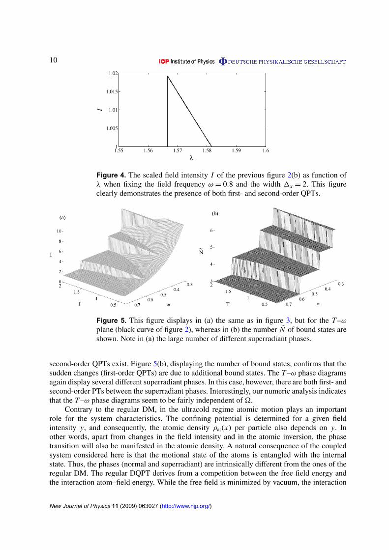
that maximizes f1(y). Thus, I is the scaled field intensity where a discontinuity in it indicates afirst-order QPT and a discontinuity in its first derivative signals a second-order QPT. Here y0 isthe lower bound, which assures at least one bound state. The parameter I corresponding to theT = 0.4 curve of figure 2(a) is presented in figure 3. We note that the ‘normal’–superradiantQPT by increasing λ is of first order, while the superradiant–‘normal’ QPT for growingλ is of second order. From the figure it is not clear if the second-order QPT is really aQPT or a cross-over. Figure 4, showing a slice (ω = 0.8) of figure 3 around one singularityλs ≈ 1.57, confirms that it is indeed a second-order QPT. Thus, contrary to the regular DQPT ofnormal–superradiance, the QPTs can be either of first- or second-order nature in this extendedDM. Figure 3 reveals not only the type of PTs of figure 2, but also that there is a number offirst-order QPTs between various superradiant phases.

Figures 3 and 4 characterize the type of QPT in the λ–ω phase diagram. The structureof the QPTs of the T –ω phase diagram turns out to be equally interesting. One example ofthe T –ω phase diagram is presented in figure 5(a). As for the λ–ω diagram, both first- and

New Journal of Physics 11 (2009) 063027 (http://www.njp.org/)

10

1.55 1.56 1.57 1.58 1.59 1.61

1.005

1.01

1.015

1.02

λ

I

Figure 4. The scaled field intensity I of the previous figure 2(b) as function ofλ when fixing the field frequency ω = 0.8 and the width 1x = 2. This figureclearly demonstrates the presence of both first- and second-order QPTs.

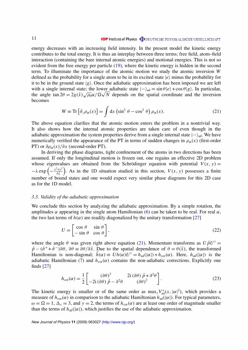
Figure 5. This figure displays in (a) the same as in figure 3, but for the T –ω

plane (black curve of figure 2), whereas in (b) the number N of bound states areshown. Note in (a) the large number of different superradiant phases.

second-order QPTs exist. Figure 5(b), displaying the number of bound states, confirms that thesudden changes (first-order QPTs) are due to additional bound states. The T –ω phase diagramsagain display several different superradiant phases. In this case, however, there are both first- andsecond-order PTs between the superradiant phases. Interestingly, our numeric analysis indicatesthat the T –ω phase diagrams seem to be fairly independent of .

Contrary to the regular DM, in the ultracold regime atomic motion plays an importantrole for the system characteristics. The confining potential is determined for a given fieldintensity y, and consequently, the atomic density ρat(x) per particle also depends on y. Inother words, apart from changes in the field intensity and in the atomic inversion, the phasetransition will also be manifested in the atomic density. A natural consequence of the coupledsystem considered here is that the motional state of the atoms is entangled with the internalstate. Thus, the phases (normal and superradiant) are intrinsically different from the ones of theregular DM. The regular DQPT derives from a competition between the free field energy andthe interaction atom–field energy. While the free field is minimized by vacuum, the interaction

New Journal of Physics 11 (2009) 063027 (http://www.njp.org/)

11

energy decreases with an increasing field intensity. In the present model the kinetic energycontributes to the total energy. It is thus an interplay between three terms; free field, atom–fieldinteraction (containing the bare internal atomic energies) and motional energies. This is not soevident from the free energy per particle (19), where the kinetic energy is hidden in the secondterm. To illuminate the importance of the atomic motion we study the atomic inversion Wdefined as the probability for a single atom to be in its excited state |e〉 minus the probability forit to be in the ground state |g〉. Once the adiabatic approximation has been imposed we are leftwith a single internal state; the lower adiabatic state |−〉ad = sin θ |e〉 + cos θ |g〉. In particular,the angle tan 2θ = 2g(x)

√ρ0α/

√N depends on the spatial coordinate and the inversion

becomes

W ≡ Tr[σzρat(x)

]=

∫dx(sin2 θ − cos2 θ

)ρat(x). (21)

The above equation clarifies that the atomic motion enters the problem in a nontrivial way.It also shows how the internal atomic properties are taken care of even though in theadiabatic approximation the system properties derive from a single internal state |−〉ad. We havenumerically verified the appearance of the PT in terms of sudden changes in ρat(x) (first-orderPT) or ∂ρat(x)/∂x (second-order PT).

In deriving the phase diagrams, tight confinement of the atoms in two directions has beenassumed. If only the longitudinal motion is frozen out, one regains an effective 2D problemwhose eigenvalues are obtained from the Schrödinger equation with potential V (x, y) =

−λ exp(−

x2+y2

12x

). As in the 1D situation studied in this section, V (x, y) possesses a finite

number of bound states and one would expect very similar phase diagrams for this 2D caseas for the 1D model.

3.3. Validity of the adiabatic approximation

We conclude this section by analyzing the adiabatic approximation. By a simple rotation, theamplitudes α appearing in the single atom Hamiltonian (6) can be taken to be real. For real α,the two last terms of h(α) are readily diagonalized by the unitary transformation [27]

U =

[cos θ sin θ

− sin θ cos θ

], (22)

where the angle θ was given right above equation (21). Momentum transforms as U pU †=

p − (σ + + σ−)∂θ , ∂θ ≡ ∂θ/∂ x . Due to the spatial dependence of θ = θ(x), the transformedHamiltonian is non-diagonal; h(α) ≡ Uh(α)U †

= had(|α|) + hcor(α). Here, had(|α|) is theadiabatic Hamiltonian (7) and hcor(α) contains the non-adiabatic corrections. Explicitly onefinds [27]

hcor(α) =1

2

[(∂θ)2 2i (∂θ) p + ∂2θ

−2i (∂θ) p − ∂2θ (∂θ)2

]. (23)

The kinetic energy is smaller or of the same order as maxx V +ad(x, |α|

2), which provides ameasure of hcor(α) in comparison to the adiabatic Hamiltonian had(|α|). For typical parameters,ω = = 1, 1x = 3, and y = 2, the terms of hcor(α) are at least one order of magnitude smallerthan the terms of had(|α|), which justifies the use of the adiabatic approximation.

New Journal of Physics 11 (2009) 063027 (http://www.njp.org/)

12

4. Longitudinal thermodynamics

In the previous section, we studied how the DQPT was modified due to motion of the atoms ina finite potential well, assuming the atomic motion to be frozen out in the longitudinal and onetransverse direction. Here we instead assume the atoms to move freely along the center axis ofthe Fabry–Perot cavity while being tightly bound in the transverse directions.

The corresponding single atom Hamiltonian (6) reads

h(α) =p2

2m+

h

2σ z + h

λ cos(µx)√

ρ0√

N

(ασ + + α∗σ−

), (24)

where µ is the scaled photon wave number, which will be set to unity hereafter, µ = 1. ThisHamiltonian, with the field still quantized, has been considered in several papers, see forexample [28]. Normally L 2π , where L is the cavity length, so neglecting boundary effectsis not a crude approximation [28]. The Hamiltonian is of the form of a generalized Mathieuequation, and hence the spectrum Eν(k) is described by a band index ν and a quasi-momentumk extending over the first Brillouin zone. Due to the internal two-level structure of the atom,the Brillouin zone is twice the size of what is imposed by the periodicity of the mode [28].Clearly, Eν(k) depends on the field amplitude α. The corresponding eigenfunctions are writtenas 8k,ν(x) = φ

(e)k,ν(x)|e〉 + φ

(g)

k,ν |g〉. For a constant coupling g(x) = λ0, these Bloch functions aresimple plane waves giving a constant energy shift independent of system parameters such as λ,ω and . For a standing wave mode coupling on the other hand, the Bloch functions cannot bedecoupled from the internal atomic states, and consequently the atomic motion will affect thestructure of the phase diagrams as will be demonstrated below.

In the previous section, we assumed the adiabatic regime and diagonalized the Hamiltonianin its internal degrees of freedom. In this case, the adiabatic potentials V ±

ad (x) cross andadiabaticity breaks down in the range where the QPTs occur. Fortunately, the Hamiltonian iseasily diagonalized numerically by truncating the dimension of the Hamiltonian matrix. Wepresent, however, asymptotic analytical results in the appendix, which rely on the adiabaticapproximation. These analytical results enable us to extract the limiting situation of large fieldamplitudes. Furthermore, as a numerical diagonalization directly renders several of the Blochbands we do not restrict the analysis to just the lowest one. However, it turns out that for mostof the presented examples only the lowest band contributes to the dynamics due to the lowtemperatures considered. Exceptions are in the plots of the critical temperature where we indeedgo to rather high temperatures and the excited bands become important.

The partition function is written like in the previous section as

Z = NC2√

Nmax

06y6∞

eN f2(y)

, (25)

where C2 is a constant and the free energy per particle

f2(y) = −βhωy + ln [g2(y)] (26)

with

g2(y) =

∞∑ν=1

∫ +1

−1dk e−βEν(k). (27)

Here, as above, y = |α|2/N represent the scaled field intensity. As shown in the appendix, the

second part of f2(y) scales asymptotically as ∼√

y for large y. Thus, a maximum of the freeenergy can only be obtained for finite or zero field intensities y.

New Journal of Physics 11 (2009) 063027 (http://www.njp.org/)

13

0 0.2 0.4 0.6 0.8 10

0.2

0.4

0.6

0.8

1.0

ω

λ c

(a)

T=3T=1

T=0.01

0 2 4 6 80.4

0.6

0.8

1.0

1.2

1.4

1.6

1.8

2.0

2.2

Ω

λ c

T=3

T=1

T=0.01

(b)

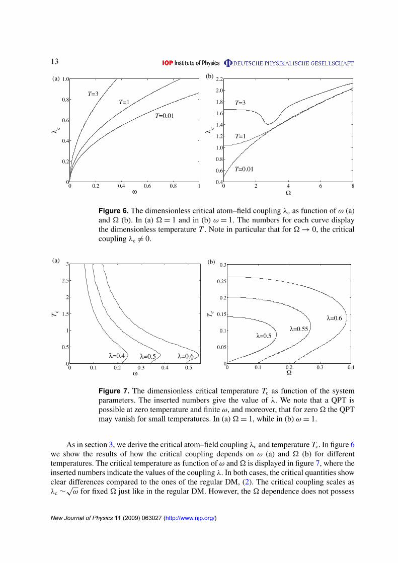
Figure 6. The dimensionless critical atom–field coupling λc as function of ω (a)and (b). In (a) = 1 and in (b) ω = 1. The numbers for each curve displaythe dimensionless temperature T . Note in particular that for → 0, the criticalcoupling λc 6= 0.

0 0.1 0.2 0.3 0.4 0.50

0.5

1

1.5

2

2.5

3

ω

Tc

λ=0.4 λ=0.5 λ=0.6

(a)

0 0.1 0.2 0.3 0.40

0.05

0.1

0.15

0.2

0.25

0.3

Ω

Tc

(b)

λ=0.5λ=0.55

λ=0.6

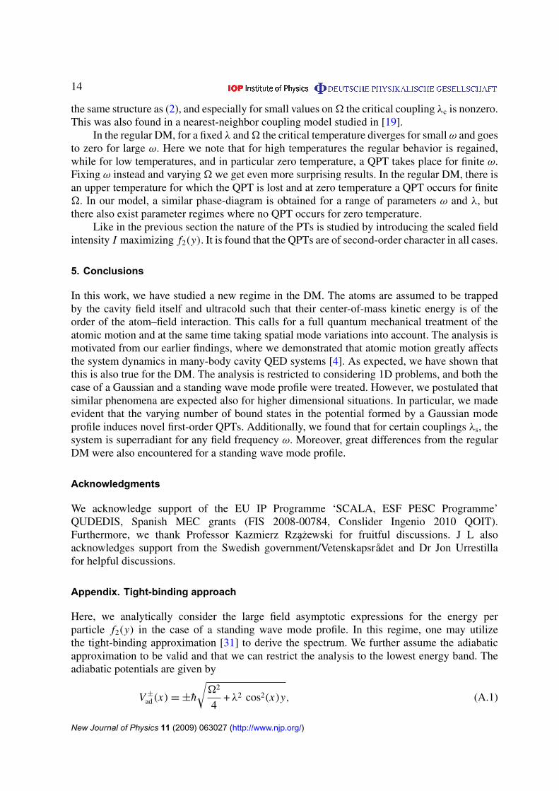
Figure 7. The dimensionless critical temperature Tc as function of the systemparameters. The inserted numbers give the value of λ. We note that a QPT ispossible at zero temperature and finite ω, and moreover, that for zero the QPTmay vanish for small temperatures. In (a) = 1, while in (b) ω = 1.

As in section 3, we derive the critical atom–field coupling λc and temperature Tc. In figure 6we show the results of how the critical coupling depends on ω (a) and (b) for differenttemperatures. The critical temperature as function of ω and is displayed in figure 7, where theinserted numbers indicate the values of the coupling λ. In both cases, the critical quantities showclear differences compared to the ones of the regular DM, (2). The critical coupling scales asλc ∼

√ω for fixed just like in the regular DM. However, the dependence does not possess

New Journal of Physics 11 (2009) 063027 (http://www.njp.org/)

14

the same structure as (2), and especially for small values on the critical coupling λc is nonzero.This was also found in a nearest-neighbor coupling model studied in [19].

In the regular DM, for a fixed λ and the critical temperature diverges for small ω and goesto zero for large ω. Here we note that for high temperatures the regular behavior is regained,while for low temperatures, and in particular zero temperature, a QPT takes place for finite ω.Fixing ω instead and varying we get even more surprising results. In the regular DM, there isan upper temperature for which the QPT is lost and at zero temperature a QPT occurs for finite. In our model, a similar phase-diagram is obtained for a range of parameters ω and λ, butthere also exist parameter regimes where no QPT occurs for zero temperature.

Like in the previous section the nature of the PTs is studied by introducing the scaled fieldintensity I maximizing f2(y). It is found that the QPTs are of second-order character in all cases.

5. Conclusions

In this work, we have studied a new regime in the DM. The atoms are assumed to be trappedby the cavity field itself and ultracold such that their center-of-mass kinetic energy is of theorder of the atom–field interaction. This calls for a full quantum mechanical treatment of theatomic motion and at the same time taking spatial mode variations into account. The analysis ismotivated from our earlier findings, where we demonstrated that atomic motion greatly affectsthe system dynamics in many-body cavity QED systems [4]. As expected, we have shown thatthis is also true for the DM. The analysis is restricted to considering 1D problems, and both thecase of a Gaussian and a standing wave mode profile were treated. However, we postulated thatsimilar phenomena are expected also for higher dimensional situations. In particular, we madeevident that the varying number of bound states in the potential formed by a Gaussian modeprofile induces novel first-order QPTs. Additionally, we found that for certain couplings λs, thesystem is superradiant for any field frequency ω. Moreover, great differences from the regularDM were also encountered for a standing wave mode profile.

Acknowledgments

We acknowledge support of the EU IP Programme ‘SCALA, ESF PESC Programme’QUDEDIS, Spanish MEC grants (FIS 2008-00784, Conslider Ingenio 2010 QOIT).Furthermore, we thank Professor Kazmierz Rzazewski for fruitful discussions. J L alsoacknowledges support from the Swedish government/Vetenskapsrådet and Dr Jon Urrestillafor helpful discussions.

Appendix. Tight-binding approach

Here, we analytically consider the large field asymptotic expressions for the energy perparticle f2(y) in the case of a standing wave mode profile. In this regime, one may utilizethe tight-binding approximation [31] to derive the spectrum. We further assume the adiabaticapproximation to be valid and that we can restrict the analysis to the lowest energy band. Theadiabatic potentials are given by

V ±

ad (x) = ±h

√2

4+ λ2 cos2(x)y, (A.1)

New Journal of Physics 11 (2009) 063027 (http://www.njp.org/)

15

where y = |α|2/N is as before the scaled field intensity. A convenient base for writing down

the periodic Hamiltonian in matrix form is to use the Wannier states w±

j (x) = 〈x | j〉w,± [31].The function w±

j (x) is localized in the j th ‘well’ of the potentials V ±

ad (x). By the tight-bindingapproximation we assume w,±〈i |h±

ad| j〉w,± = 0 unless i = j or i = j ± 1. Within the validityregime of this approximation we may as well replace the Wannier functions by Gaussianfunctions [4]. The widths of the Gaussians are given by approximating the potential wells byharmonic oscillators, giving

w±

j (x) ≈ w±

G(x − x j) ≡1

4√

πσ 2e−[(x−x j )

2/2σ 2], (A.2)

where

σ 2=

(∂2V ±

ad (x)

∂x2

∣∣∣∣x=x j

)−1

(A.3)

and x j is the position of the j th potential well. To avoid un-physical contributions from thenon-orthogonality of the Gaussians we impose

∫dx wG(x − x j)wG(x − xi) = δi j . We further

introduce the matrix elements

Ei(y) =

∫∞

−∞

dx w±

G∗(x−x j)

(−

1

2

∂2

∂x2

)w±

G(x−x j+i),

J ±

i (y)=

∫∞

−∞

dx w±

G∗(x−x j)V ±

ad (x, |α|2)w±

G(x−x j+i),

(A.4)

where we only consider i = 0, 1. We note that the Wannier functions are directly related tothe depth of the corresponding potential and therefore their width σ will also depend on y.This explains the field intensity dependence of Ei(y). Another important observation is thatw±

G(x − x j) are localized where |V ±

ad (x)| are close either to their maxima or minima, resultingin different coupling elements J ±

i (y), indicated by the ±-superscript. In this notation we get thelowest band tight-binding energy

E±

1 (k) = E0(y) + J ±

0 (y) +[E1(y) + J ±

1 (y)]

2 cos(k). (A.5)

The part in front of the cosine function is strictly negative resulting in the ground-state energybeing given by k = 0. The kinetic energy integrals of (A.4) are readily solvable, and one finds

E0(y) =1

4σ 2,

E1(y) = −1

8σ 4exp

(−

π 2

4σ 2

) (2σ 2 + π2

).

(A.6)

The potential integrals of (A.4) are not analytically solvable for the given potentials (A.1).Instead we make the same kind of approximation as in section 3

V ±

ad (x) ≈ ±A ± B cos2(x), (A.7)

New Journal of Physics 11 (2009) 063027 (http://www.njp.org/)

16

and identify

A =

2,

B =

√2

4+ λ2 y −

2.

(A.8)

Within this regime we find

J ±

0 (y) = ±

2+

1

4√

mσ 2

(1 ∓ e−σ 2

),

J ±

1 (y) = ±1

4σ 2e−π2/4σ 2

e−σ 2.

(A.9)

We emphasize that the width σ 2 depends on the field intensity y;

σ 2=

1

2B. (A.10)

The applied approximations are only reliable for z < 1 [4], and it turns out that the QPTsoccur beyond these approximations. Nonetheless, we may find the asymptotics for the freeenergy f2(y). In the large y limit, we find that ln [g2(y)] ∼

√y. Consequently, the field intensity

I will always be finite, regardless of parameter choices. We have verified numerically the ysquare-root dependence of ln [g2(y)] for large intensities.

References

[1] Meystre P 2001 Atom Optics (Berlin: Springer)Metcalf H J and van der Straten P 2001 Laser Cooling and Trapping (Berlin: Springer)

[2] Slama S, Krentz G, Bux S, Zimmermann C and Courteille P W 2007 Phys. Rev. A 75 063620Brennecke F, Donner T, Ritter S, Bourdel T, Köhn M and Esslinger T 2007 Nature 450 268Truetlein P, Hunger D, Camerer S, Hänsch T and Reichel J 2007 Phys. Rev. Lett. 99 140403Colombe Y, Steinmetz T, Dubois G, Linke F, Hunger D and Reichel J 2007 Nature 450 272Brennecke F, Ritter S, Donner T and Esslinger T 2008 Science 322 235

[3] Machler C and Ritsch H 2005 Phys. Rev. Lett. 95 260401[4] Lewenstein M, Kubasiak A, Larson J, Menotti C, Morigi G, Osterloh K and Sanpera A 2006 Proc. ICAP—

2006 (AIP Conference Series vol 869) ed C F Roos, H Häffner and R Blatt (Melville, NY: AIP) pp 201–11Larson J, Damski B, Morigi G and Lewenstein M 2008 Phys. Rev. Lett. 100 050401Larson J, Fernandez-Vidal S, Morigi G and Lewenstein M 2008 New J. Phys. 10 045002Larson J, Morigi G and Lewenstein M 2008 Phys. Rev. A 78 023815

[5] Sachdev S 2006 Quantum Phase Transitions (Cambridge: Cambridge University Press)[6] Jarret T C, Lee C F and Johnson N F 2006 Phys. Rev. B 74 121301

Lee C F and Johnson N F 2008 Europhys. Lett. 81 37004Chen G, Wang X, Liang J-Q and Wang Z D 2008 Phys. Rev. A 78 023634Morrison S and Parkins A S 2008 Phys. Rev. Lett. 100 040403Morrison S and Parkins A S 2008 Phys. Rev. A 77 043810

[7] Dicke R H 1954 Phys. Rev. 93 99[8] Larson J and Martikainen J-P 2008 Phys. Rev. A 78 063618

Larson J and Martikainen J-P 2008 arXiv:0811.4147

New Journal of Physics 11 (2009) 063027 (http://www.njp.org/)

17

[9] Kozierowski M and Chumakov S M 1995 Phys. Rev. A 52 4194Chumakov S M and Kozierowski M 1996 Quantum Semiclass. Opt. 8 775Castro-Beltran H M, Sanchez-Mondragon J J and Chumakov S M 1998 Opt. Commun. 15 348Ramon G, Brif C and Mann A 1998 Phys. Rev. A 58 2506

[10] Zhan Y B 1992 Phys. Lett. A 167 441Seke J 1995 Physica A 213 587Shindo D, Chavez A, Chumakov S M and Klimov A B 2004 J. Opt. B: Quantum Semiclass. Opt. 6 1464

[11] Doherty G and Jex I 1993 Opt. Commun. 102Schneider S and Milburn G J 2002 Phys. Rev. A 65 042107Nemes M C, Furuya K, Pellegrino G Q, Oliveira A C, Reis M and Sanz L 2006 Phys. Lett. A 354 60

[12] Agarwal G S, Puri R R and Singh R P 1997 Phys. Rev. A 56 2249Klimov A B and Saavedra C 1998 Phys. Lett. A 247 14

[13] Wang Y K and Hioe F T 1973 Phys. Rev. A 7 831Hepp K and Lieb E H 1973 Ann. Phys. NY 76 360Hepp K and Lieb E H 1973 Phys. Rev. A 8 2517Lee B S 1976 J. Phys. A: Math. Gen. 9 573

[14] Mallory W R 1975 Phys. Rev. A 11 1088[15] Orszag M 1977 J. Phys. A: Math. Gen. 10 1995[16] Chagas E A and Furuya K 2008 Phys. Lett. A 372 5564[17] Hioe F T 1973 Phys. Rev. A 8 1440

Orszag M 1976 J. Phys. A: Math. Gen 10 L21Seke J 1993 Physica A 193 587

[18] Gilmore R 1976 Phys. Lett. A 55 459Provost J P, Rocca F, Vallee G and Sirugae M 1976 Physica A 85 2002Sun C C and Bowden C M 1979 J. Phys. A: Math. Gen. 12 2273Puri R R, Lawande S V and Hassan S S 1980 Opt. Commun. 35 179Pan F, Wang T, Pan J, Li Y F and Dranger J P 2005 Phys. Lett. A 341 94Li Y, Wang Z D and Sun C P 2006 Phys. Rev. A 74 023815Lukyanets S P and Bevzenko D A 2006 Phys. Rev. A 74 053803Chen G, Zhao D and Chen Z 2006 J. Phys. B: At. Mol. Opt. Phys. 39 3315Tolkunov D and Solenov D 2007 Phys. Rev. B 75 024402Goto H and Ichimura K 2008 Phys. Rev. A 77 053811

[19] Lee C F and Johnson N F 2004 Phys. Rev. Lett. 93 083001[20] Resken J, Quinoga L and Johnson N F 2005 Europhys. Lett. 69 8

Liberti G, Plastina F and Piperno F 2006 Phys. Rev. A 74 022324Jarret T C, Oloya-Castro A and Johnson N F 2006 Europhys. Lett. 77 34001

[21] Emary C and Brandes T 2003 Phys. Rev. Lett. 90 044101Emary C and Brandes T 2003 Phys. Rev. E 67 066203Lambert N, Emary C and Brandes T 2004 Phys. Rev. Lett. 92 073602Vidal J and Dusuel S 2006 Europhys. Lett. 74 817Chen G, Li J Q and Liang J-Q 2006 Phys. Rev. A 74 054101

[22] Dimer F, Estienne B, Parkings A S and Carmichael H J 2007 Phys. Rev. A 75 013804[23] Al-Saidi W A and Stroud D 2002 Phys. Rev. B 65 224512

Chen G, Chen Z and Liang J 2007 Phys. Rev. A 76 055803[24] Rzazewski K, Wódkiewicz K and Zakowicz W 1975 Phys. Rev. Lett. 35 432[25] Białynicki-Birula I and Rzazewski K 1979 Phys. Rev. A 19 301

Gawedzki K and Rzazewski K 1981 Phys. Rev. A 23 2134[26] Englert B G, Schwinger J., Barut A O and Scully M O 1991 Europhys. Lett. 14 25

Meyer G M, Scully M O and Walther H 1997 Phys. Rev. A 56 4142

New Journal of Physics 11 (2009) 063027 (http://www.njp.org/)

18

Bastin T and Martin J 2003 Phys. Rev. A 67 053804Larson J 2009 J. Phys. B: At. Mol. Opt. Phys. 42 044015

[27] Larson J and Stenholm S 2006 Phys. Rev. A 73 033805Larson J 2007 Phys. Scr. 76 146Baer M 2006 Beyond Born–Oppenheimer (New York: Wiley)

[28] Compagno G, Peng J S and Persico F 1982 Phys. Rev. A 26 2065Ren W and Carmichael H J 1995 Phys. Rev. A 51 752Vaglica A 1995 Phys. Rev. A 52 2319Hood C J, Chapman M S, Lynn T W and Kimble H J 1998 Phys. Rev. A 80 4157Larson J, Salo J and Stenholm S 2005 Phys. Rev. A 72 013814Larson J 2006 Phys. Rev. A 73 013823

[29] Landau L D and Lifshitz E M 1991 Quantum Mechanics (Oxford: Pergamon)[30] Arfken G B and Weber H J 2001 Mathematical Methods For Physicists (San Deigo: Harcourt Academic)

Hayek S I 2001 Advanced Mathematical Methods in Science and Enginering (New York: Marcel Dekker)[31] Ascroft N W and Mermin N D 1976 Solid State Physics (New York: Harcourt Collage)

New Journal of Physics 11 (2009) 063027 (http://www.njp.org/)