Embed Size (px)
Citation preview
DigitalSnow Final meeting
Digital Level Layers for Curve Decomposition and Vectorization
Yan Gerard (ISIT) [email protected]
july 9th 2015, Autrans
DLL decomposition
Digital Level Layers
Introduction
About tangent estimators
Plan
2
Algorithm

Introduction
Plan
3

Building
(3D printer, factory…) Computer simulation
(Finite Elements Methods…)
Images (video games, movies, FX,
Augmented Reality…)
Real world data acquisition (3D-scanners, computer vision,
motion capture, medical imaging…)
Geometric design (3D artists, designers…)
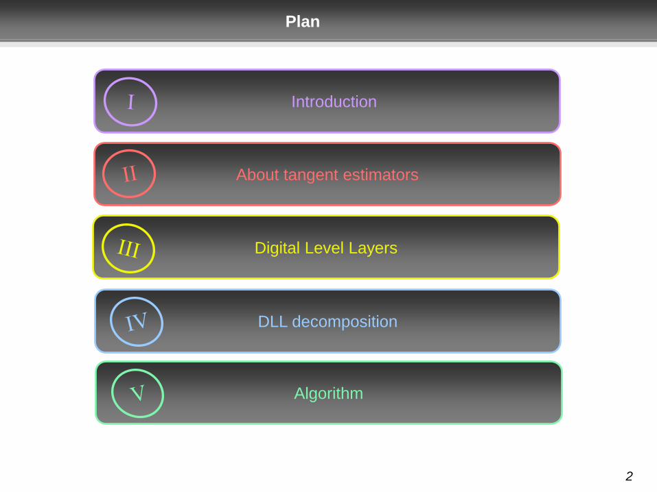
3D models (geometry)
Martin Newell’s
Utah Teapot
Introduction 3D Workflows
3D models (geometry)
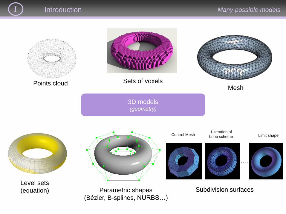
Introduction Many possible models
Points cloud
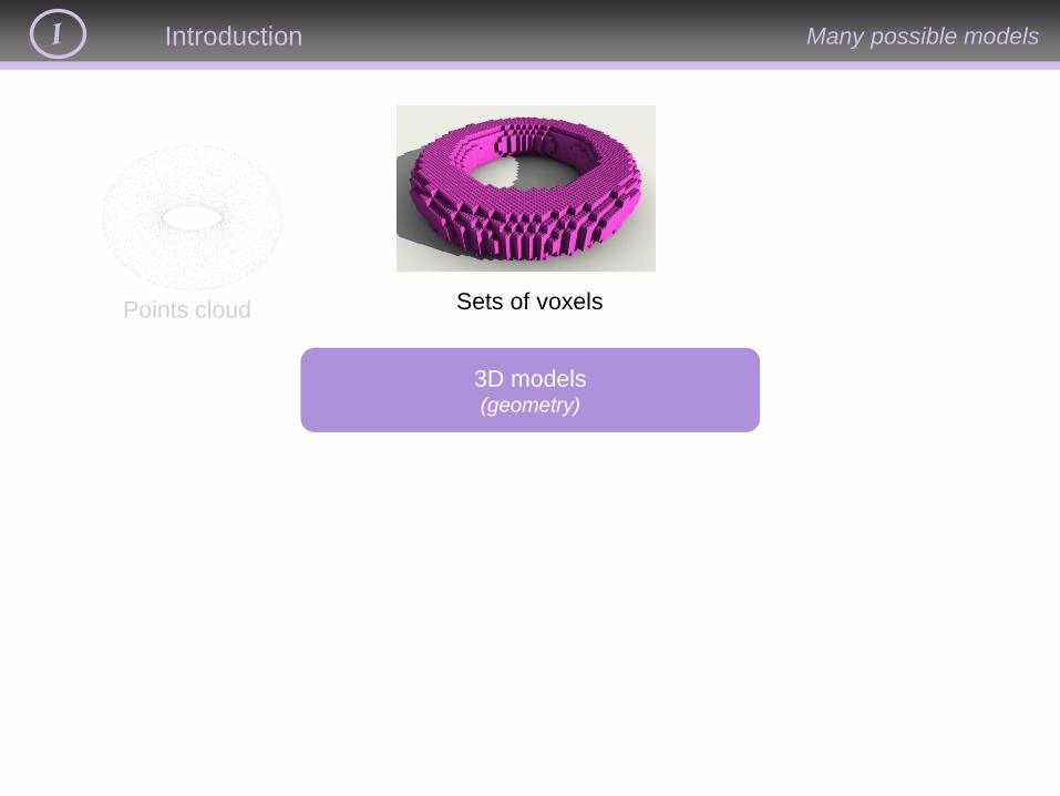
3D models (geometry)
Introduction
Points cloud Sets of voxels
Many possible models
3D models (geometry)
Introduction
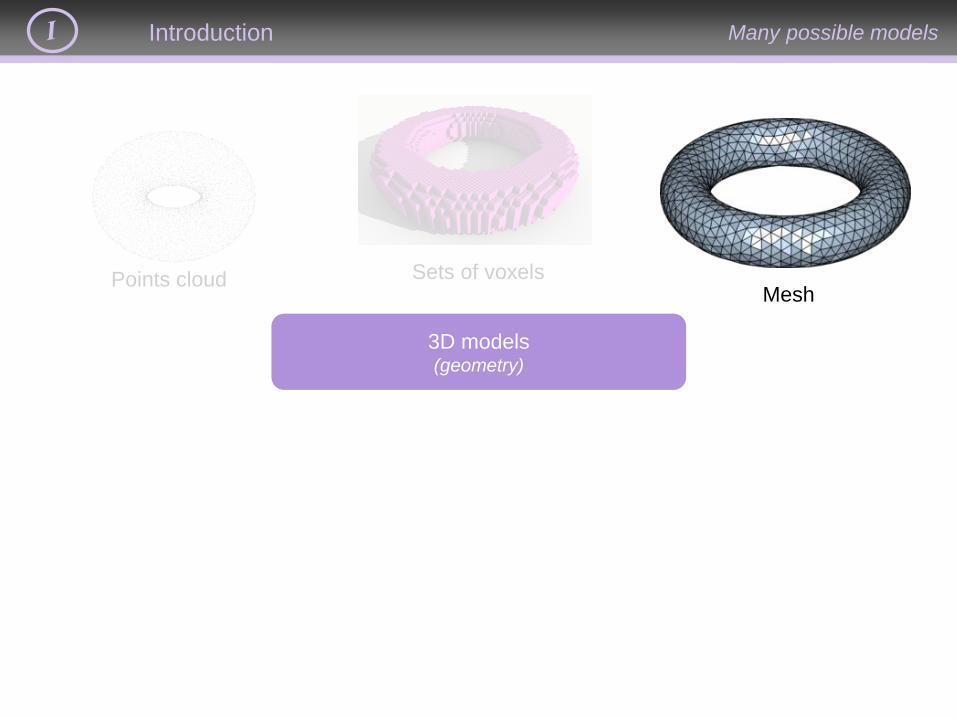
Points cloud Sets of voxels Mesh
Many possible models
3D models (geometry)
Introduction
Points cloud Sets of voxels Mesh
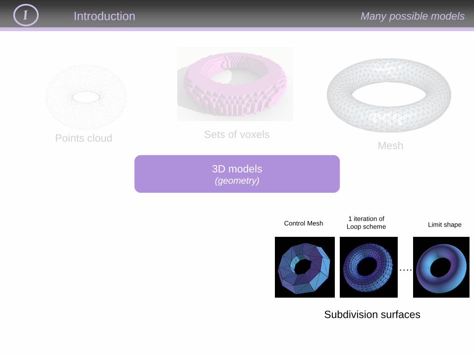
Subdivision surfaces
Control Mesh 1 iteration of
Loop scheme Limit shape
….
Many possible models

3D models (geometry)
Introduction
Points cloud Sets of voxels Mesh
Subdivision surfaces
Control Mesh 1 iteration of
Loop scheme Limit shape
….
Many possible models
Parametric shapes
(Bézier, B-splines, NURBS…)
3D models (geometry)
Introduction
Points cloud Sets of voxels Mesh
Subdivision surfaces
Control Mesh 1 iteration of
Loop scheme Limit shape
….
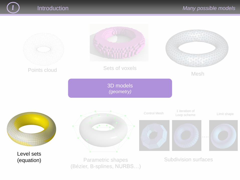
Many possible models
Parametric shapes
(Bézier, B-splines, NURBS…)
Level sets
(equation)
3D models (geometry)
Introduction
Points cloud Sets of voxels Mesh
Subdivision surfaces
Control Mesh 1 iteration of
Loop scheme Limit shape
….
Many possible models
Parametric shapes
(Bézier, B-splines, NURBS…)
Level sets
(equation)
3D models (geometry)
Introduction
Points cloud Sets of voxels Mesh
Subdivision surfaces
Control Mesh 1 iteration of
Loop scheme Limit shape
….
Parametric shapes
(Bézier, B-splines, NURBS…)
Level sets
(equation)
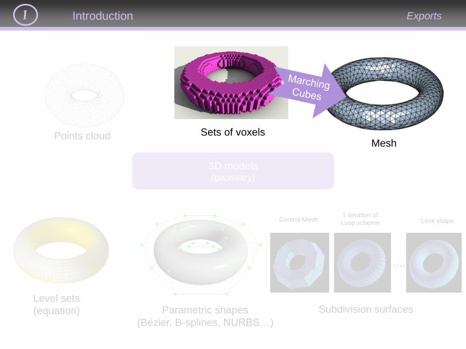
Exports

Just export the digital model in a mesh with marching cubes and simplification.
Introduction
Sets of voxels
Export vs stubborn people
That’s the option followed by most people
(it’s a good option). But some people are stubborn.
Let me my voxels!!!

Introduction Legos castle
But some people are stubborn.
May be, they played to much legos during
their childhood.
Are there some better reasons to do Digital Geometry ?
Let me my voxels!!!

Introduction Beauty?
For the beauty of theory
A stepped surface @ Thomas Fernique
Are there some better reasons to do Digital Geometry ?
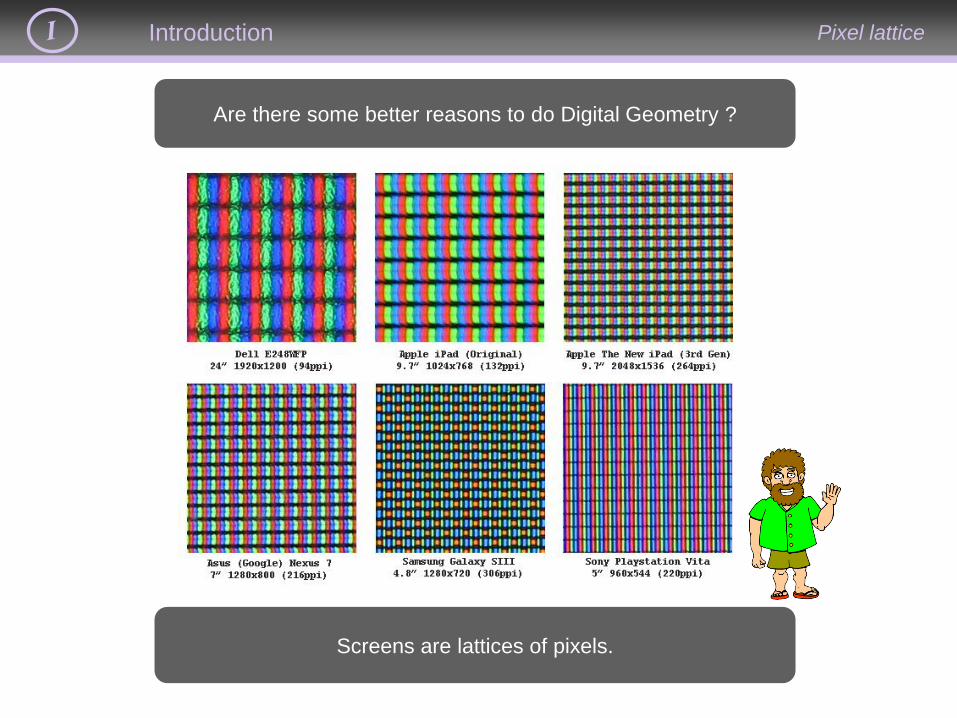
Introduction Pixel lattice
Are there some better reasons to do Digital Geometry ?
Screens are lattices of pixels.

Introduction A better reason to do Digital Geometry?
Binary image
Images are tabs of pixel values.
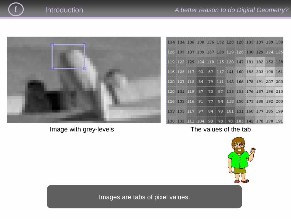
Introduction A better reason to do Digital Geometry?
Image with grey-levels The values of the tab
Images are tabs of pixel values.

Introduction A better reason to do Digital Geometry?
RGB image
Images are tabs of pixel values.

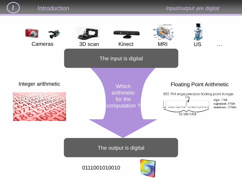
Introduction Input/output are digital
Cameras 3D scan Kinect MRI US
The output is digital
0111001010010
Computation
The input is digital
…
Introduction Input/output are digital
Cameras 3D scan Kinect MRI US
The output is digital
0111001010010
The input is digital
…
Which
arithmetic
for the
computation ?
Integer arithmetic Floating Point Arithmetic

Introduction Input/output are digital
Integer arithmetic Floating Point Arithmetic
Suitable for computers
(exact computations)
Suitable for mathematics
(continuous objects)
Requires digital mathematics… Problems of inaccuracy…

Introduction Input/output are digital
Floating Point Arithmetic
Suitable for mathematics
(continuous objects)
Problems of inaccuracy…
y=ln(1-x)/x
with IEEE 754 standard

Introduction Integers VS floats
Output = integers
Use
integer
arithmetic
Input = integers
(or integers multiplied by a fixed resolution)
Use
Floating point
numbers
with suitable
digital
mathematical
theories
and
classical
continuous
Mathematics
(and do as there
was no problem of
accuracy)
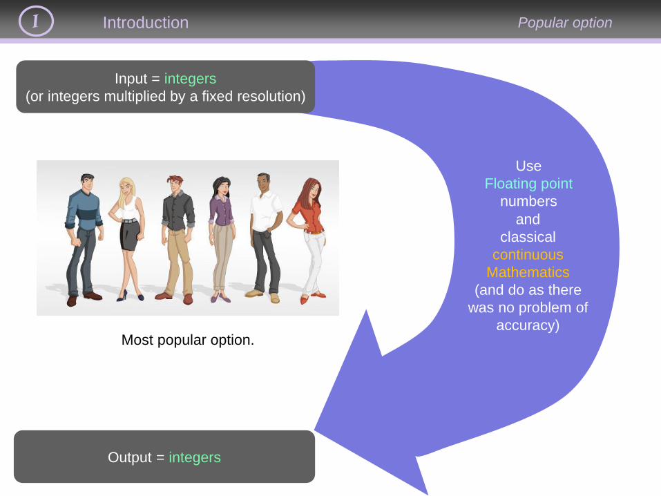
Introduction
Output = integers
Input = integers
(or integers multiplied by a fixed resolution)
Most popular option.
Popular option
Use
Floating point
numbers
and
classical
continuous
Mathematics
(and do as there
was no problem of
accuracy)

Introduction The challenge of digital mathematics
Output = integers
Use
integer
arithmetic
Input = integers
(or integers multiplied by a fixed resolution)
with suitable
digital
mathematical
theories
The developpment of
digital mathematics
is a huge challenge
We can not do whatever
we want. There are
some constraints…
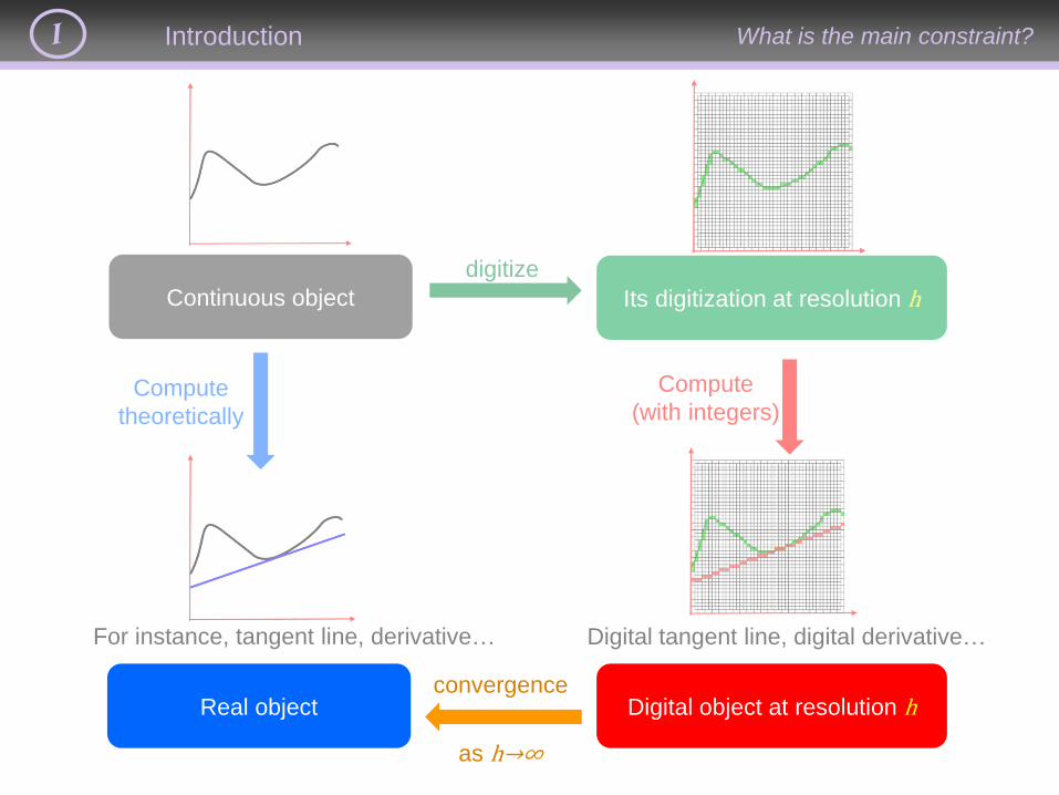
Introduction What is the main constraint?
Continuous object Its digitization at resolution h digitize
Compute
theoretically
Real object
For instance, tangent line, derivative…
Compute
(with integers)
Digital object at resolution h
Digital tangent line, digital derivative…
convergence
as h→∞

Measurements
Digital Primitives
Introduction
About tangent estimators
Plan
28
Transformations and Combinatorics
Plan
About tangent estimators
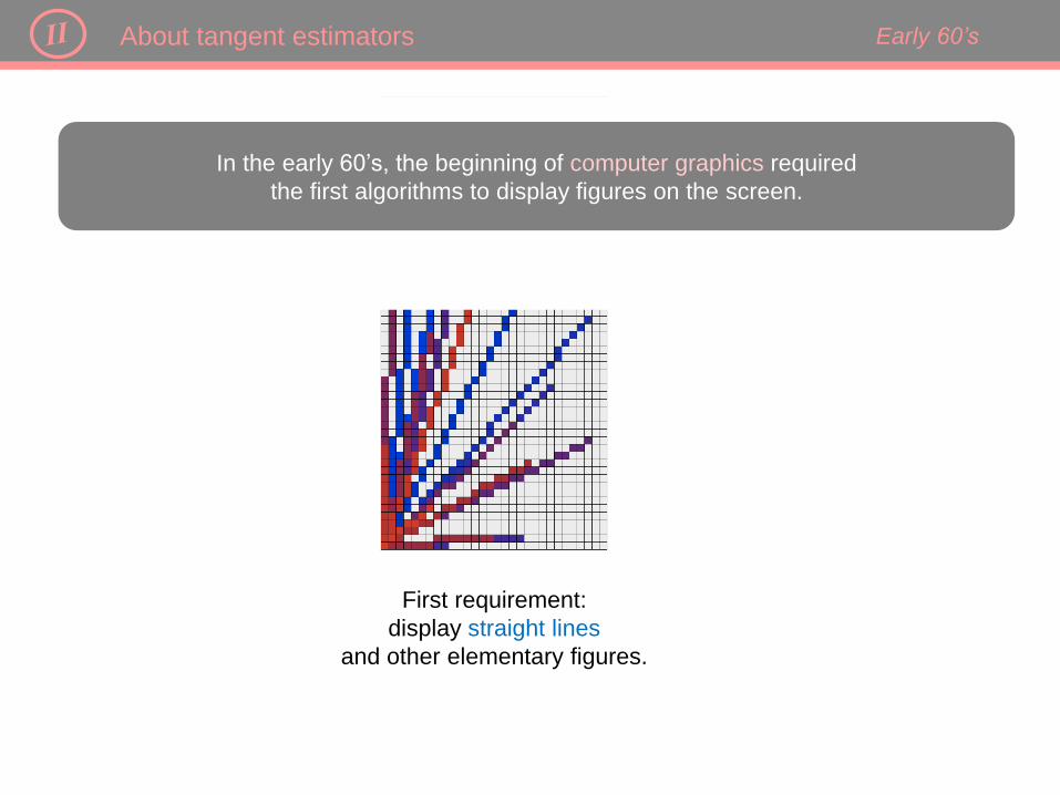
First requirement:
display straight lines
and other elementary figures.
In the early 60’s, the beginning of computer graphics required
the first algorithms to display figures on the screen.
Early 60’s About tangent estimators
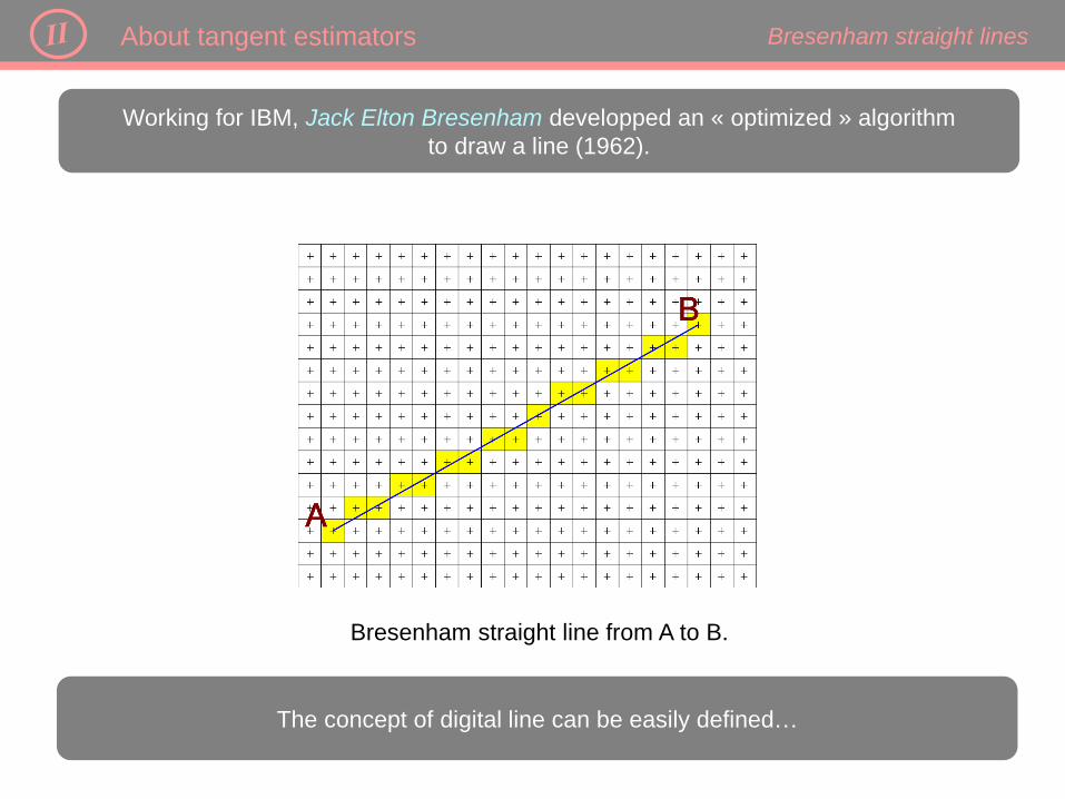
Bresenham straight line from A to B.
Working for IBM, Jack Elton Bresenham developped an « optimized » algorithm
to draw a line (1962).
The concept of digital line can be easily defined…
Bresenham straight lines About tangent estimators

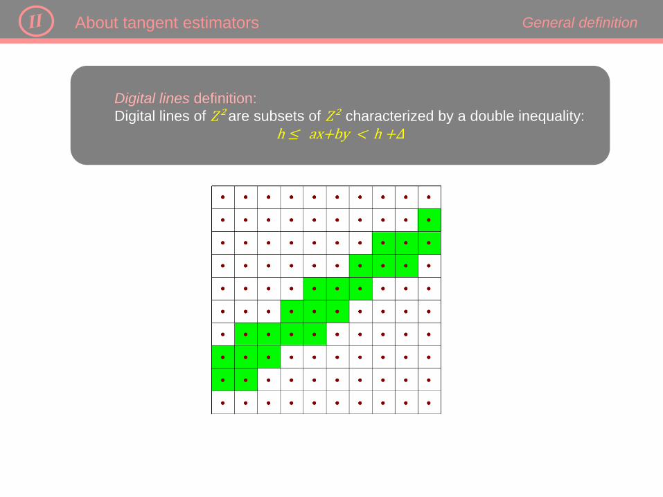
Digital lines definition:
Digital lines of Z² are subsets of Z² characterized by a double inequality:
h ≤ ax+by < h +Δ
It’s exactly the same for affine
sub-spaces of codimension 1
(digital hyperplanes) of Zd.
Definition About tangent estimators
Digital lines definition:
Digital lines of Z² are subsets of Z² characterized by a double inequality:
h ≤ ax+by < h +Δ
ax+by=h
ax+by=h+Δ
General definition About tangent estimators

A digital line is naïve if Δ =max{|a|,|b|} .
It’s 8-connected.
Digital lines definition:
Digital lines of Z² are subsets of Z² characterized by a double inequality:
h ≤ ax+by < h +Δ
Naïve lines
The complementary has two 4-connected components.
There is no simple point.
About tangent estimators

A digital line is standard if Δ =|a|+|b| .
It’s 4-connected.
Digital lines definition:
Digital lines of Z² are subsets of Z² characterized by a double inequality:
h ≤ ax+by < h +Δ
Standard lines
The complementary has two 8-connected components.
There is no simple point.
About tangent estimators
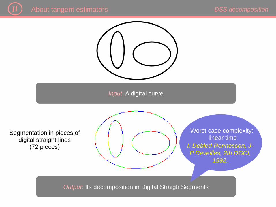
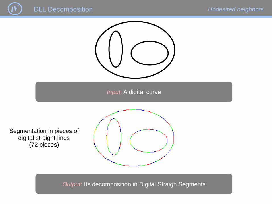
Input: A digital curve
DSS decomposition
Output: Its decomposition in Digital Straigh Segments
Segmentation in pieces of digital straight lines
(72 pieces)
Worst case complexity: linear time
I. Debled-Rennesson, J-
P Reveilles, 2th DGCI,
1992.
About tangent estimators

Input: A digital curve
Tangential Cover
Output: Its Tangential Cover
That’s the Tangential COVER
Worst Case Complexity: Linear Time
J-O Lachaud, A. Vialard, F. De Vieilleville, DGCI 2005.
About tangent estimators
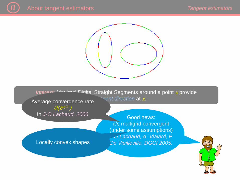
Tangent estimators
Interest: Maximal Digital Straight Segments around a point x provide
the tangent direction at x.
Good news:
it’s multigrid convergent
(under some assumptions)
J-O Lachaud, A. Vialard, F.
De Vieilleville, DGCI 2005.
Average convergence rate
O(h2/3 ) In J-O Lachaud, 2006
Locally convex shapes
About tangent estimators

Tangent estimators
Interest: Maximal Digital Straight Segments around a point x provide
the tangent direction at x.
There exist other ways to
provide multigrid convergent
tangent estimators…
About tangent estimators

40
Curvatures of curves and surfaces
Why this interest for computing the tangent or normal direction ?
α
Tangent
and
normal
directions
Angles
Local Measurements About tangent estimators
To provide measurements…
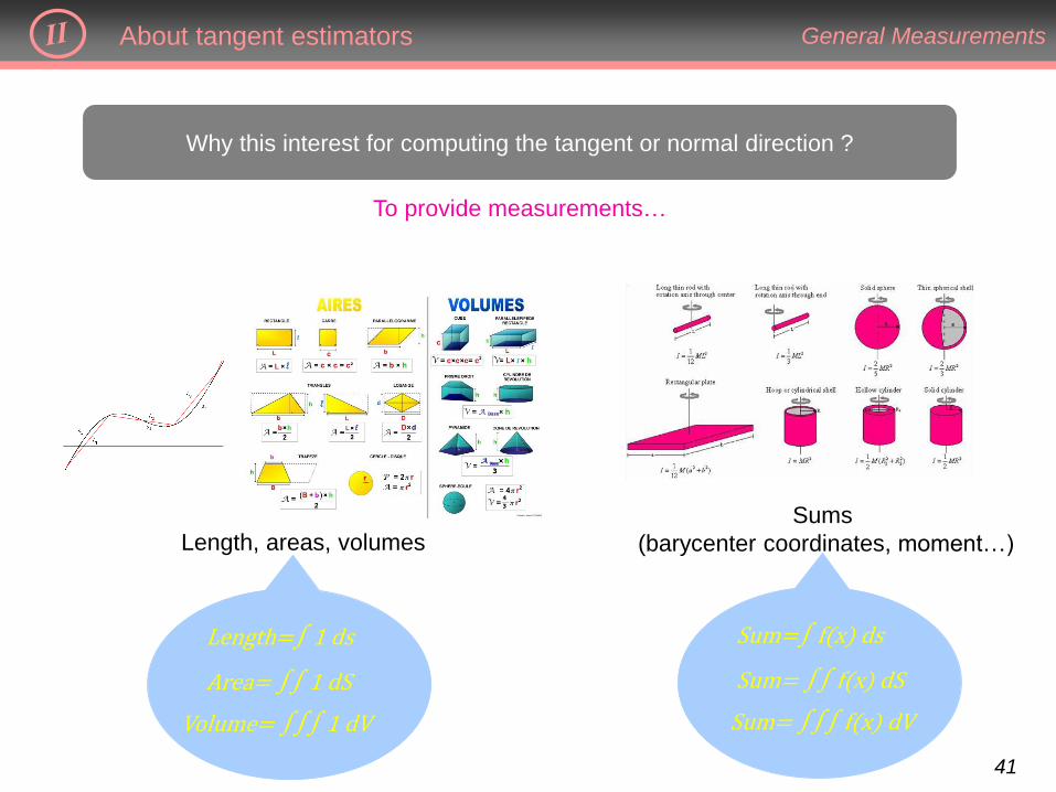
41
Length, areas, volumes Sums
(barycenter coordinates, moment…)
Length=∫ 1 ds
Area= ∫∫ 1 dS
Volume= ∫∫∫ 1 dV
Sum=∫ f(x) ds
Sum= ∫∫ f(x) dS
Sum= ∫∫∫ f(x) dV
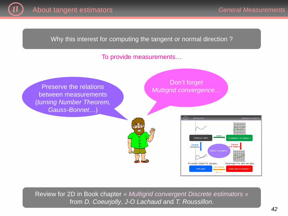
General Measurements About tangent estimators
To provide measurements…
Why this interest for computing the tangent or normal direction ?
42
Preserve the relations
between measurements
(turning Number Theorem,
Gauss-Bonnet…)
Don’t forget
Multigrid convergence…
General Measurements
Review for 2D in Book chapter « Multigrid convergent Discrete estimators »
from D. Coeurjolly, J-O Lachaud and T. Roussillon.
About tangent estimators
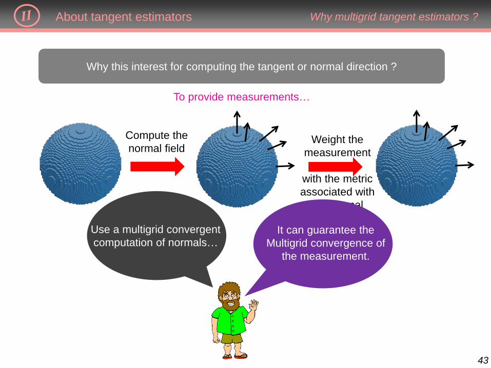
To provide measurements…
Why this interest for computing the tangent or normal direction ?
43
Compute the
normal field Weight the
measurement
with the metric
associated with
the normal
Use a multigrid convergent
computation of normals… It can guarantee the
Multigrid convergence of
the measurement.
Why multigrid tangent estimators ? About tangent estimators
To provide measurements…
Why this interest for computing the tangent or normal direction ?

44
Better ideas ?
Everything is cool, but…
Can we do better than using digital straight segments ?
Not only for tangent estimation, but also for conversion from raster to vector graphics.
Use digital primitives of higher degree .
About tangent estimators

45
Better ideas ?
Curvature is defined with
osculating circles
Use digital circles
An analytical function is approximated by
its Taylor Polynomial of degree n.
Use a more generic approach
About tangent estimators
Use digital primitives of higher degree .
46
Better ideas ?
Use a more generic approach
About tangent estimators

DLL decomposition
Digital Level Layers
Introduction
About tangent estimators
Plan
47
Algorithm

Digital Level Layers
Plan
48

Usual geometry is based on real numbers, which by paradox are ’’unreal’’.
limit
Numbers with a
finite description
and a finite time…
World of Reals.
Different discrete objects or concepts have the same limit …
There is not only one way to
discretize a real concept…
Warning Digital Level Layers
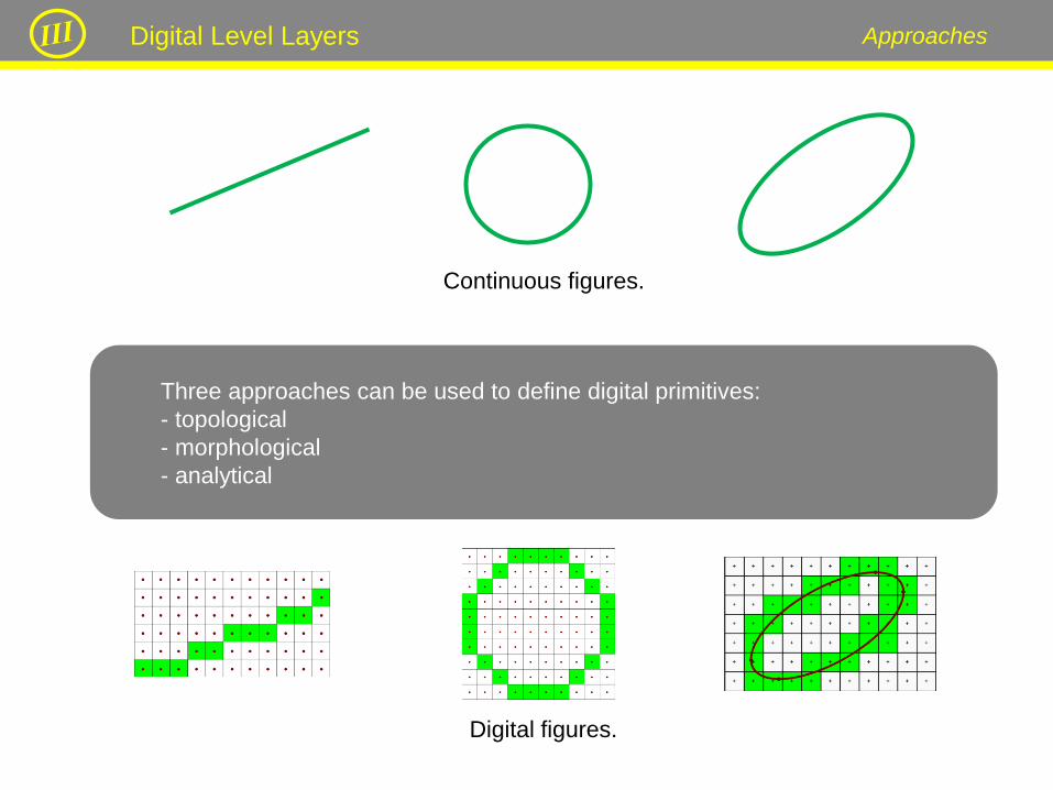
Three approaches can be used to define digital primitives:
- topological
- morphological
- analytical
Approaches
Continuous figures.
Digital figures.
Digital Level Layers

Task: define a digital primitive for S.
Illustration on an ellipse Digital Level Layers

Task: define a digital primitive for S.
Topological ellipse Digital Level Layers

53
A shape S
A structuring element B
The Minkowski’s sum S+B is the set of points covered by the structuring elements
as it moves all along the shape.
Minkowski’s sum Digital Level Layers

54
A shape S
A structuring element B The dilation of S by B
The Minkowski’s sum S+B is the set of points covered by the structuring elements
as it moves all along the shape.
Minkowski’s sum Digital Level Layers
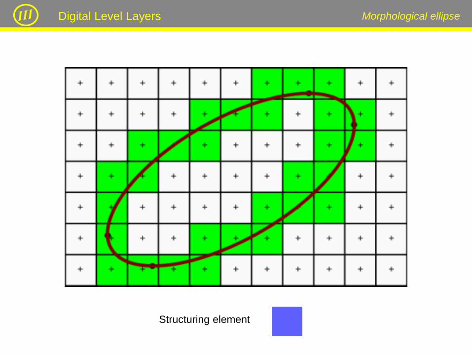
Structuring element
Morphological ellipse Digital Level Layers

We relax the equality f(x)=h in a double inequality h-Δ/2 ≤ f(x)<h +Δ/2.
Analytical ellipse Digital Level Layers
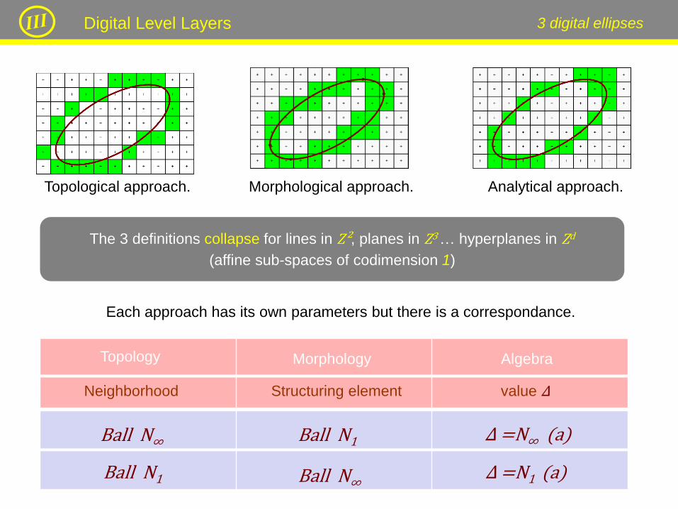
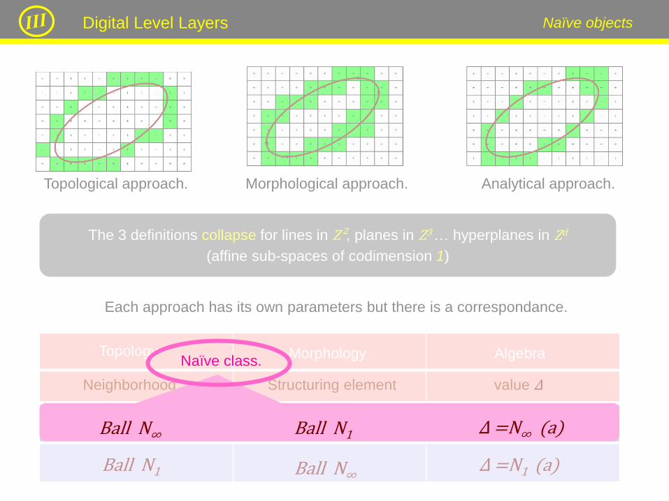
The 3 definitions collapse for lines in Z², planes in Z3 … hyperplanes in Zd
(affine sub-spaces of codimension 1)
3 digital ellipses
Topological approach. Morphological approach. Analytical approach.
Each approach has its own parameters but there is a correspondance.
Topology Morphology Algebra
Neighborhood Structuring element value Δ
Ball N∞ Ball N1 Δ =N∞ (a)
Ball N1 Ball N∞ Δ =N1 (a)
Digital Level Layers
The 3 definitions collapse for lines in Z², planes in Z3 … hyperplanes in Zd
(affine sub-spaces of codimension 1)
Naïve objects
Topological approach. Morphological approach. Analytical approach.
Each approach has its own parameters but there is a correspondance.
Topology Morphology Algebra
Neighborhood Structuring element value Δ
Ball N1 Ball N∞ Δ =N1 (a)
Ball N∞ Ball N1 Δ =N∞ (a)
Naïve class.
Digital Level Layers
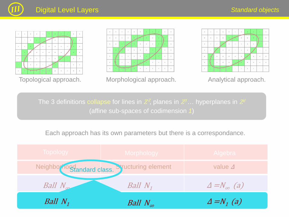
The 3 definitions collapse for lines in Z², planes in Z3 … hyperplanes in Zd
(affine sub-spaces of codimension 1)
Topological approach. Morphological approach. Analytical approach.
Each approach has its own parameters but there is a correspondance.
Topology Morphology Algebra
Neighborhood Structuring element value Δ
Ball N∞ Ball N1 Δ =N∞ (a)
Ball N1 Ball N∞ Δ =N1 (a)
Standard class.
Standard objects Digital Level Layers
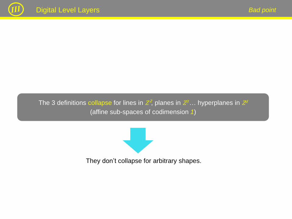
Bad point
The 3 definitions collapse for lines in Z², planes in Z3 … hyperplanes in Zd
(affine sub-spaces of codimension 1)
They don’t collapse for arbitrary shapes.
Digital Level Layers
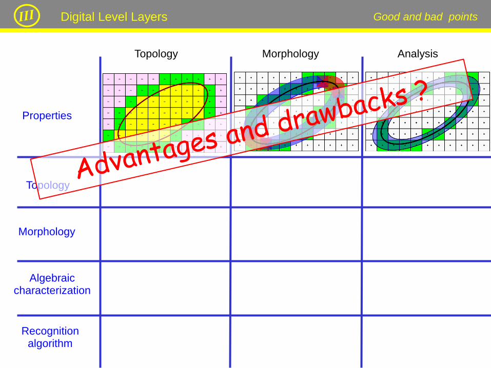
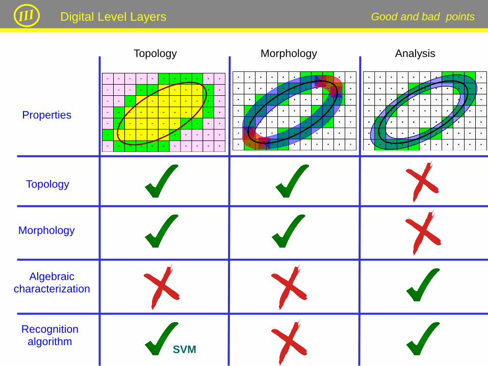
Topology Morphology Analysis
Topology
Morphology
Algebraic characterization
Recognition algorithm
Properties
Good and bad points Digital Level Layers
Topology Morphology Analysis
Topology
Morphology
Algebraic characterization
Recognition algorithm
Properties
SVM
Good and bad points Digital Level Layers
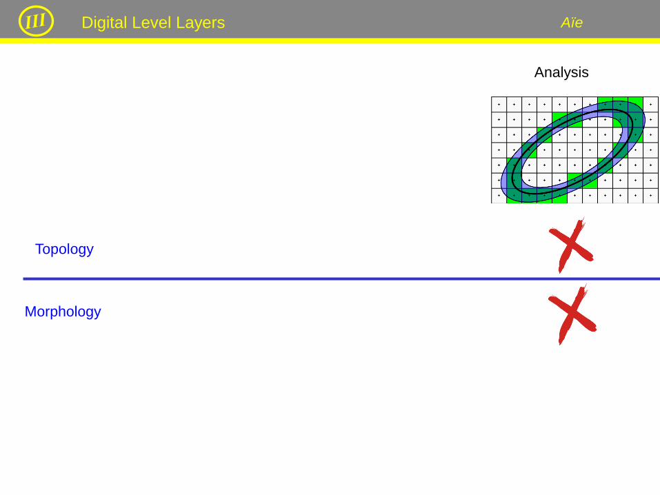
Topology
Morphology
Aïe
Analysis
Digital Level Layers

Topology
Morphology
Digital Level Layer definition:
A Digital Level Layer (name coming from Level sets) is a subset of Z d characterized by a double inequality:
h ≤ f(x) < h’
Definition
Analysis
Digital Level Layers
Digital Level Layer definition:
A Digital Level Layer (name coming from Level sets) is a subset of Z d characterized by a double inequality:
h ≤ f(x) < h’
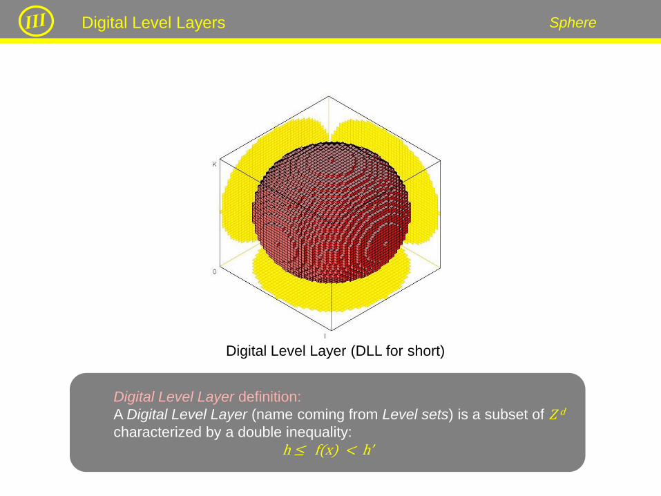
Digital Level Layer (DLL for short)
Sphere Digital Level Layers
Digital Level Layer definition:
A Digital Level Layer (name coming from Level sets) is a subset of Z d characterized by a double inequality:
h ≤ f(x) < h’
Digital Level Layer (DLL for short)
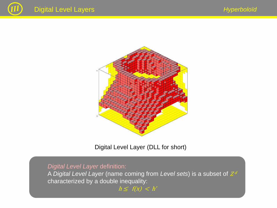
Hyperboloïd Digital Level Layers
Digital Level Layer definition:
A Digital Level Layer (name coming from Level sets) is a subset of Z d characterized by a double inequality:
h ≤ f(x) < h’
Digital Level Layer (DLL for short)
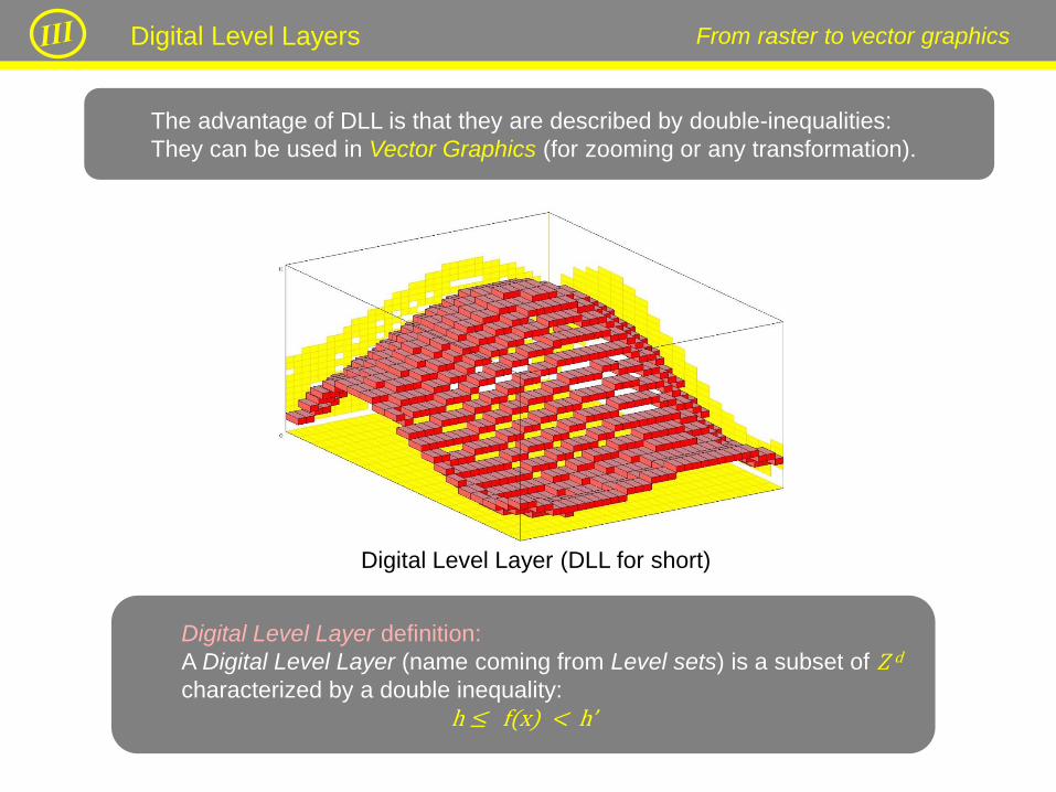
The advantage of DLL is that they are described by double-inequalities:
They can be used in Vector Graphics (for zooming or any transformation).
From raster to vector graphics Digital Level Layers
Digital Level Layer definition:
A Digital Level Layer (name coming from Level sets) is a subset of Z d characterized by a double inequality:
h ≤ f(x) < h’
Theoretical results ? Digital Level Layers
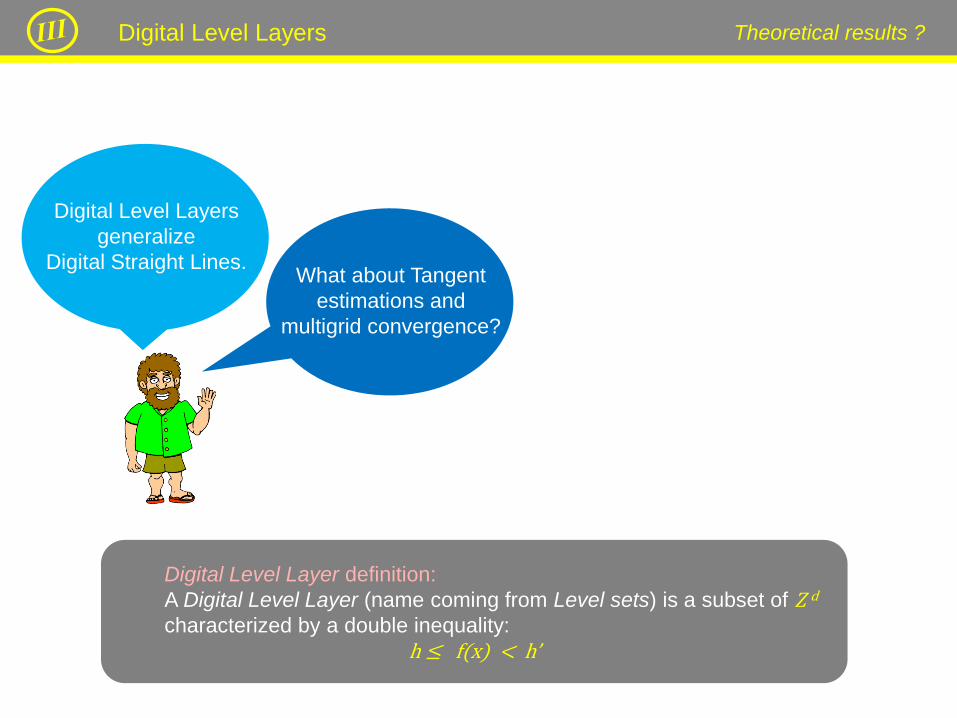
Digital Level Layers
generalize
Digital Straight Lines. What about Tangent
estimations and
multigrid convergence?
Derivatives estimators Digital Level Layers
Method Authors
Assumption
on the continuous
curve
Order
of
derivative
Worst case
Error bound
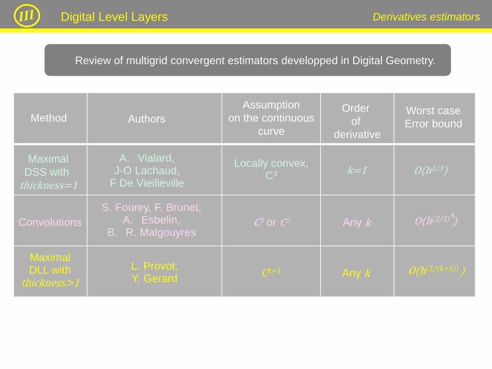
O(h(1/(k+1)) ) Maximal DLL with
thickness>1
L. Provot, Y. Gerard
Ck+1 Any k
Maximal
DSS with
thickness=1
A. Vialard, J-O Lachaud,
F De Vieilleville
Locally convex, C3 k=1 O(h1/3)
S. Fourey, F. Brunet, A. Esbelin,
B. R. Malgouyres Convolutions C3 or C2 Any k O(h(2/3) )
k
Review of multigrid convergent estimators developped in Digital Geometry.

Derivatives estimators Digital Level Layers
Method Authors
Assumption
on the continuous
curve
Order
of
derivative
Worst case
Error bound
S. Fourey, F. Brunet, A. Esbelin,
B. R. Malgouyres Convolutions C3 or C2
O(h(1/(k+1)) )
Any k O(h(2/3) ) k
Maximal DLL with
thickness>1
L. Provot, Y. Gerard
Ck+1 Any k
Parameter free
because the parameter
i.e the class of digital
straight lines has been
fixed…
Maximal
DSS with
thickness=1
A. Vialard, J-O Lachaud,
F De Vieilleville
Locally convex, C3 k=1 O(h1/3)
Review of multigrid convergent estimators developped in Digital Geometry.

Derivatives estimators Digital Level Layers
Method Authors
Assumption
on the continuous
curve
Order
of
derivative
Worst case
Error bound
S. Fourey, F. Brunet, A. Esbelin,
B. R. Malgouyres Convolutions C3 or C2 Any k O(h(2/3) )
k
O(h(1/(k+1)) ) Maximal DLL with
thickness>1
L. Provot, Y. Gerard
Ck+1 Any k
Maximal
DSS with
thickness=1
A. Vialard, J-O Lachaud,
F De Vieilleville
Locally convex, C3 k=1 O(h1/3)
Review of multigrid convergent estimators developped in Digital Geometry.
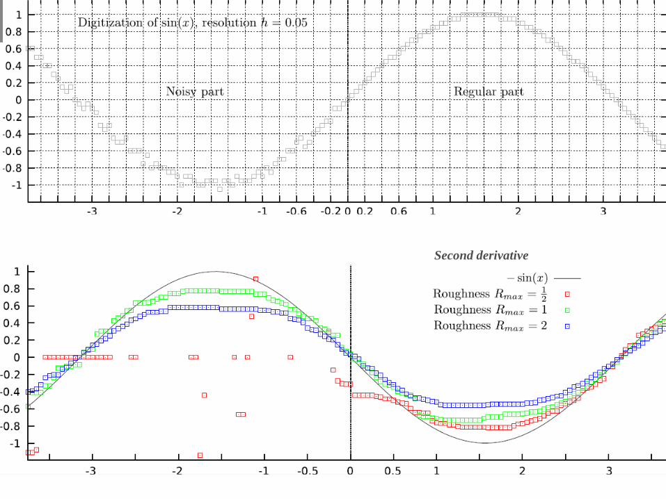
All approaches are able to
deal with noisy shapes
(using their parameters).
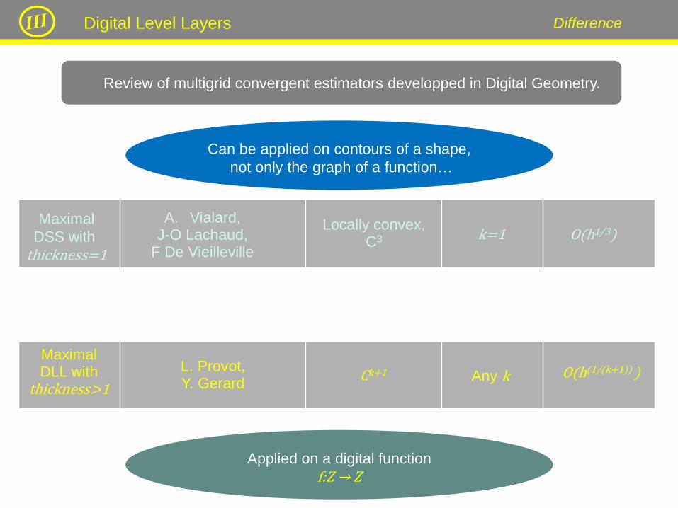
Difference Digital Level Layers
Maximal
DSS with
thickness=1
A. Vialard, J-O Lachaud,
F De Vieilleville
Locally convex, C3 k=1 O(h1/3)
S. Fourey, F. Brunet, A. Esbelin,
B. R. Malgouyres
O(h(1/(k+1)) ) Maximal DLL with
thickness>1
L. Provot, Y. Gerard
Ck+1 Any k
Review of multigrid convergent estimators developped in Digital Geometry.
Can be applied on contours of a shape,
not only the graph of a function…
Applied on a digital function
f:Z → Z
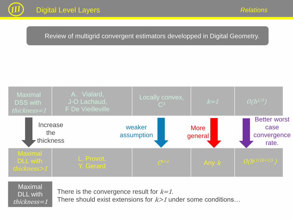
Relations Digital Level Layers
Maximal
DSS with
thickness=1
A. Vialard, J-O Lachaud,
F De Vieilleville
Locally convex, C3 k=1 O(h1/3)
S. Fourey, F. Brunet, A. Esbelin,
B. R. Malgouyres Convolutions C3 or C2
O(h(1/(k+1)) )
Any k O(h(2/3) ) k
Maximal DLL with
thickness>1
L. Provot, Y. Gerard
Ck+1 Any k
Better worst
case
convergence
rate.
Increase
the
thickness
weaker
assumption More
general
Maximal DLL with
thickness=1
There is the convergence result for k=1.
There should exist extensions for k>1 under some conditions…
Review of multigrid convergent estimators developped in Digital Geometry.

Relations Digital Level Layers
Method
Maximal
DSS with
thickness=1
Authors
Assumption
on the continuous
curve
Order
of
derivative
A. Vialard, J-O Lachaud,
F De Vieilleville
Locally convex, C3 k=1 O(h1/3)
S. Fourey, F. Brunet, A. Esbelin,
B. R. Malgouyres Convolutions C3 or C2
O(h(1/(k+1)) )
Any k O(h(2/3) ) k
Maximal DLL with
thickness>1
L. Provot, Y. Gerard
Ck+1 Any k
Computation in worst case linear time for a single DLL.
Computation in O(n2(k+1)) in theory but close to linear time in practice for a single DLL.
Iterative version with deleting and points insertion for computing the derivative along a curve.
It remains linear.
No iterative version with deleting and points insertion for computing the derivative along a
curve. It becomes quadratic.
Review of multigrid convergent estimators developped in Digital Geometry.

Relations Digital Level Layers
Maximal
DSS with
thickness=1
A. Vialard, J-O Lachaud,
F De Vieilleville
Locally convex, C3 k=1 O(h1/3)
S. Fourey, F. Brunet, A. Esbelin,
B. R. Malgouyres Convolutions C3 or C2
O(h(1/(k+1)) )
Any k O(h(2/3) ) k
Maximal DLL with
thickness>1
L. Provot, Y. Gerard
Ck+1 Any k
More restrictive and less accurate but faster…
Review of multigrid convergent estimators developped in Digital Geometry.
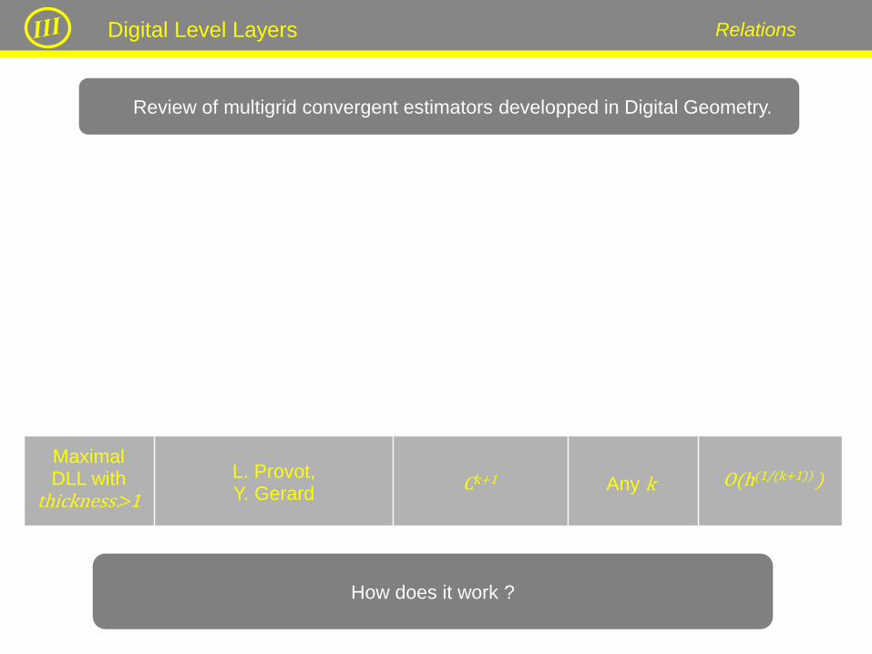
Relations Digital Level Layers
Method Authors Order
of
derivative
Worst case
Error bound
O(h(1/(k+1)) ) Maximal DLL with
thickness>1
L. Provot, Y. Gerard
Ck+1 Any k
How does it work ?
Review of multigrid convergent estimators developped in Digital Geometry.
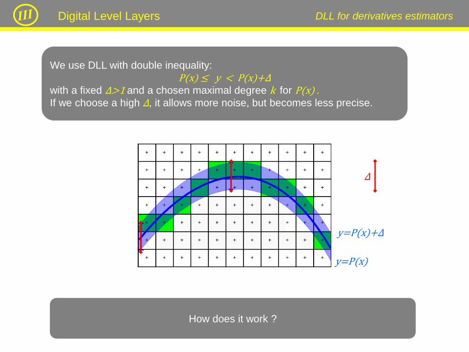
DLL for derivatives estimators Digital Level Layers
We use DLL with double inequality:
P(x) ≤ y < P(x)+Δ
with a fixed Δ>1 and a chosen maximal degree k for P(x) . If we choose a high Δ, it allows more noise, but becomes less precise.
Δ
How does it work ?
y=P(x)
y=P(x)+Δ

DLL for derivatives estimators Digital Level Layers
We use DLL with double inequality:
P(x) ≤ y < P(x)+Δ
with a fixed Δ>1 and a chosen maximal degree k for P(x) . If we choose a high Δ, it allows more noise, but becomes less precise.
Δ
P(x) provides directly the derivative of order k.
y=P(x)
y=P(x)+Δ
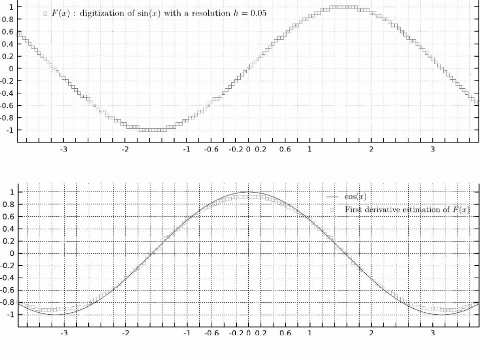
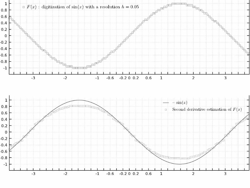
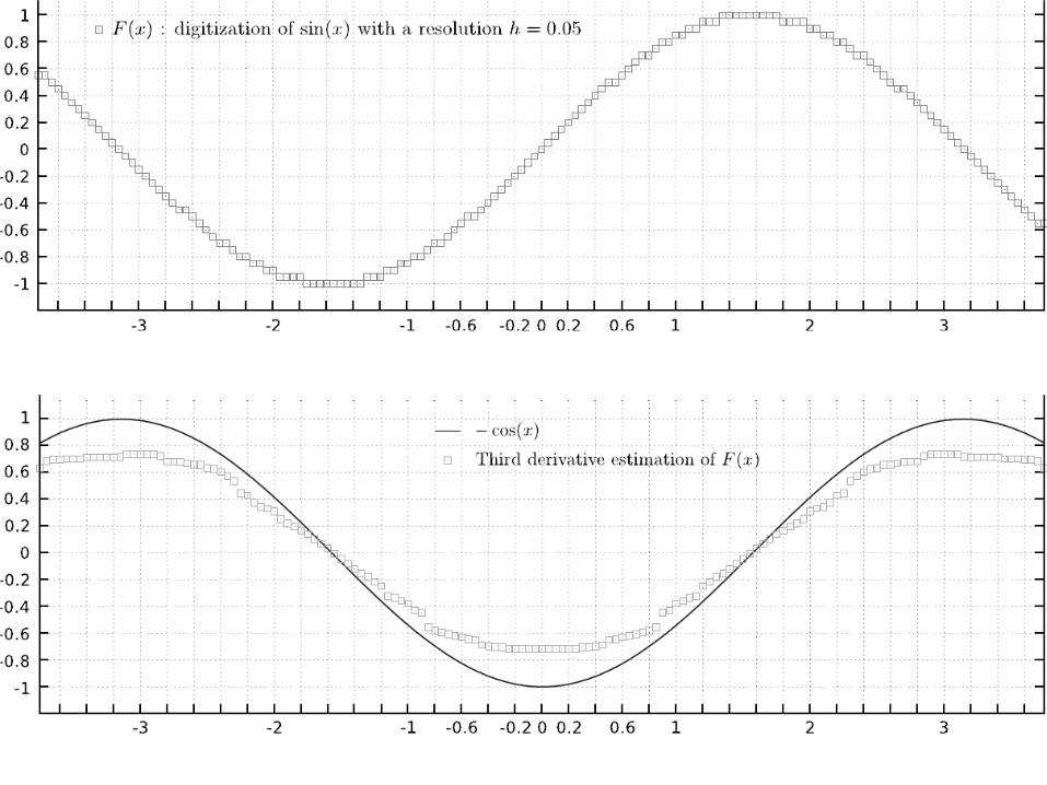
Second derivative
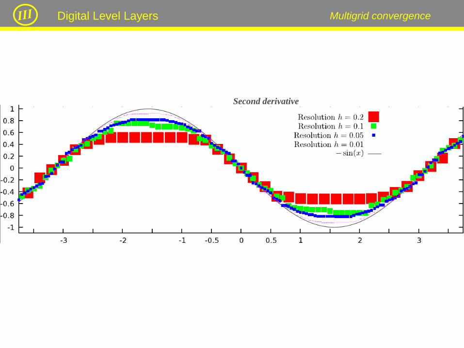
Second derivative
Multigrid convergence Digital Level Layers

DLL decomposition
Digital Level Layers
Introduction
About tangent estimators
Plan
84
Algorithm

DLL decomposition
Plan
85
Input: A digital curve
Output: Its decomposition in Digital Straigh Segments
Segmentation in pieces of digital straight lines
(72 pieces)
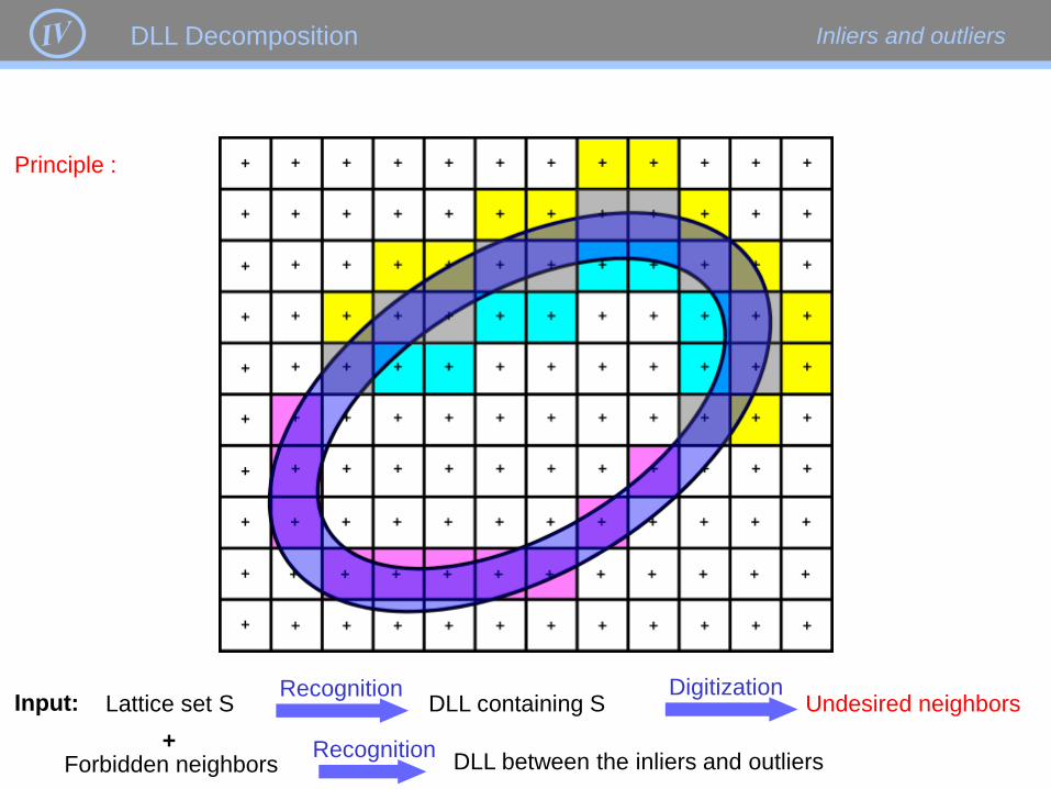
Undesired neighbors DLL Decomposition

Principle :
Lattice set S Input: Recognition
DLL containing S Digitization
Undesired neighbors
Undesired neighbors DLL Decomposition
Principle :
Lattice set S Input: Recognition
DLL containing S Digitization
Undesired neighbors
Forbidden neighbors + Recognition
DLL between the inliers and outliers
Inliers and outliers DLL Decomposition
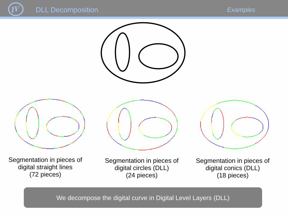
Segmentation in pieces of digital straight lines
(72 pieces)
Segmentation in pieces of digital circles (DLL)
(24 pieces)
Segmentation in pieces of digital conics (DLL)
(18 pieces)
Examples
We decompose the digital curve in Digital Level Layers (DLL)
DLL Decomposition
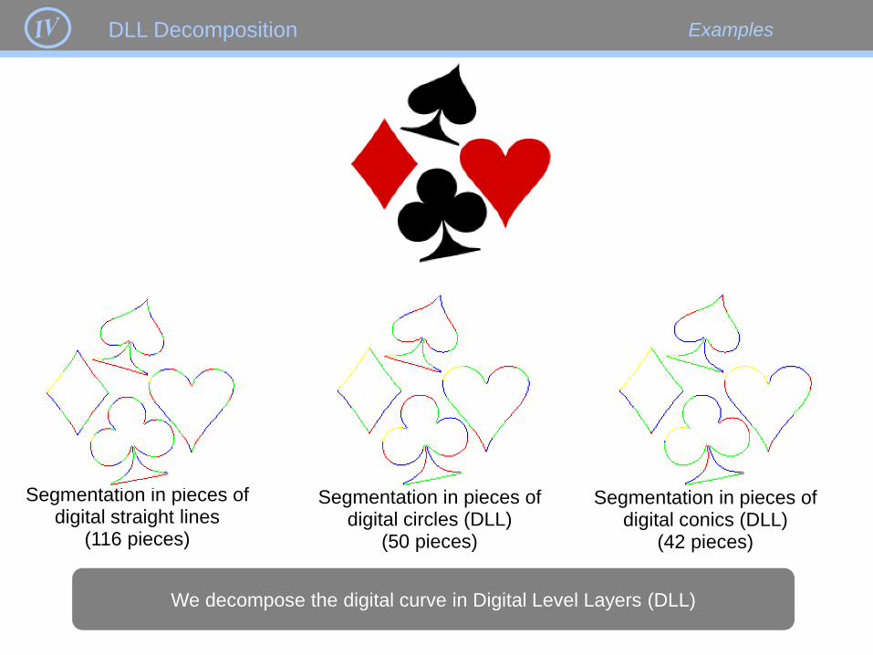
Segmentation in pieces of digital straight lines
(116 pieces)
Segmentation in pieces of digital circles (DLL)
(50 pieces)
Segmentation in pieces of digital conics (DLL)
(42 pieces)
We decompose the digital curve in Digital Level Layers (DLL)
Examples DLL Decomposition

Segmentation in pieces of digital straight lines
(116 pieces)
Segmentation in pieces of digital circles (DLL)
(50 pieces)
Segmentation in pieces of digital conics (DLL)
(42 pieces)
It provides a vector description of a digital curve wich is smoother than DSS.
Examples DLL Decomposition
All cases computed with a UNIQUE algorithm
(with, as parameter, a chosen basis of polynomials like in SVM)

IPOL DLL Decomposition
Paper, Demo and code are available on IPOL (thanks to Bertrand Kerautret)

DLL decomposition
Digital Level Layers
Introduction
About tangent estimators
Plan
93
Algorithm

Plan
94
Algorithm
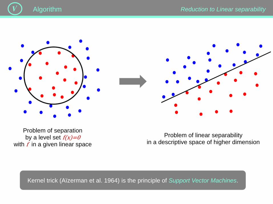
Problem of separation by a level set f(x)=0
with f in a given linear space
Problem of linear separability in a descriptive space of higher dimension
Reduction to Linear separability Algorithm
Kernel trick (Aïzerman et al. 1964) is the principle of Support Vector Machines.
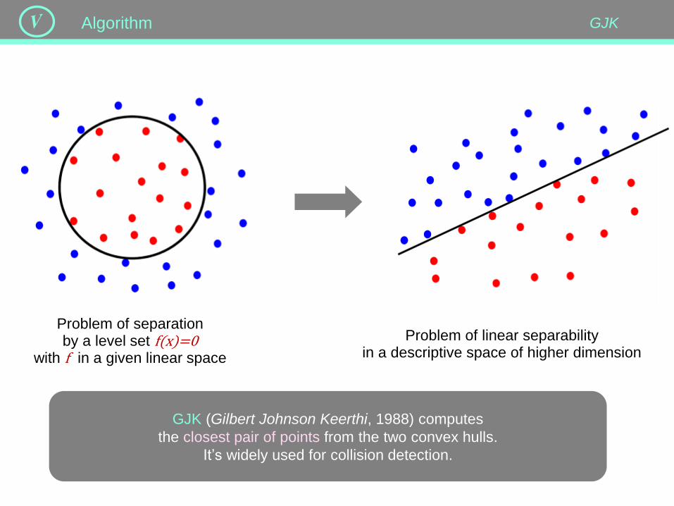
Problem of separation by a level set f(x)=0
with f in a given linear space
GJK Algorithm
GJK (Gilbert Johnson Keerthi, 1988) computes
the closest pair of points from the two convex hulls.
It’s widely used for collision detection.
Problem of linear separability in a descriptive space of higher dimension

Problem of separation by two level sets f(x)=h and f(x)=h’
with f in a given linear space
Problem of linear separability by two parallel hyperplanes
We introduce a variant of GJK in nD
Variant with three sets of points Algorithm
GJK (Gilbert Johnson Keerthi, 1988) computes
the closest pair of points from the two convex hulls.
It’s widely used for collision detection.

Input : two polytopes A⊂Rd and B⊂Rd given by their vertices.
Question : do they intersect ?
More general question: compute their minimal distance.
A and B Difference A -B
A
B
A -B
distance (A,B)=distance(0,A-B)
Principe of GJK algorithm :
compute the distance between the origin O and B-A.
GJK Algorithm

Principe of GJK algorithm :
compute the distance between the origin O and B-A.
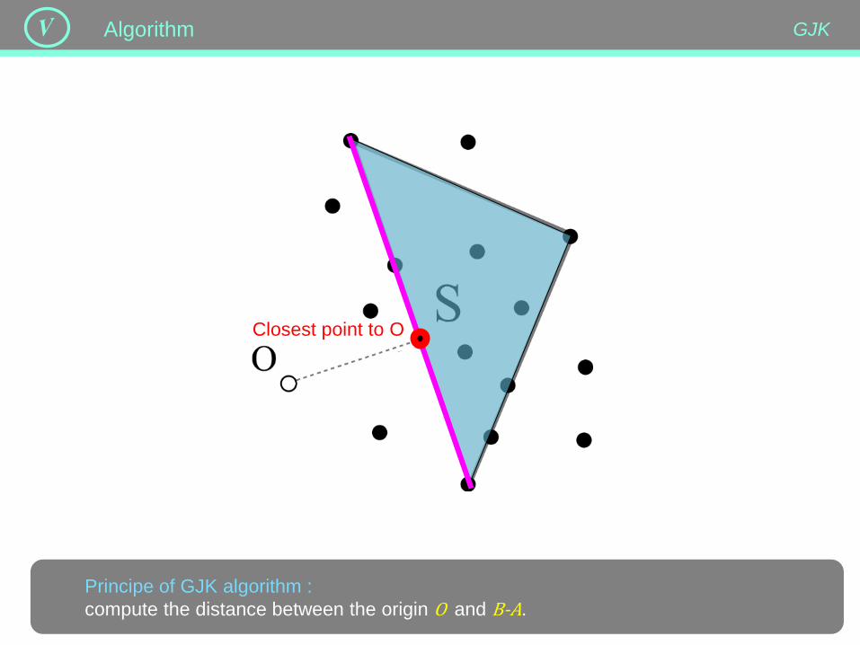
GJK Algorithm

Principe of GJK algorithm :
compute the distance between the origin O and B-A.
GJK Algorithm
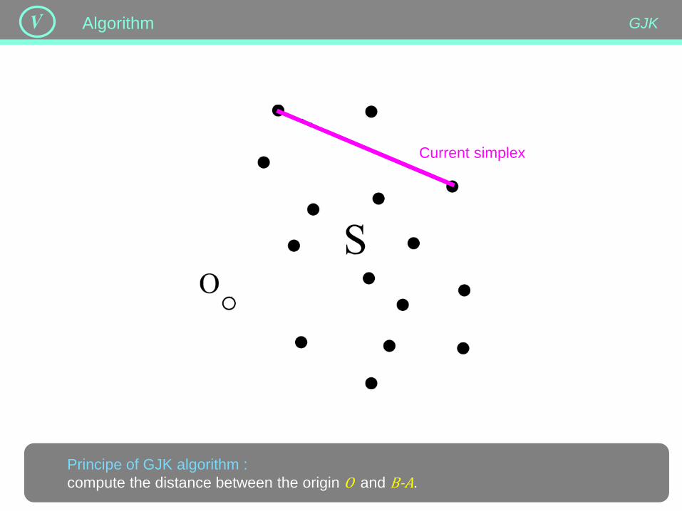
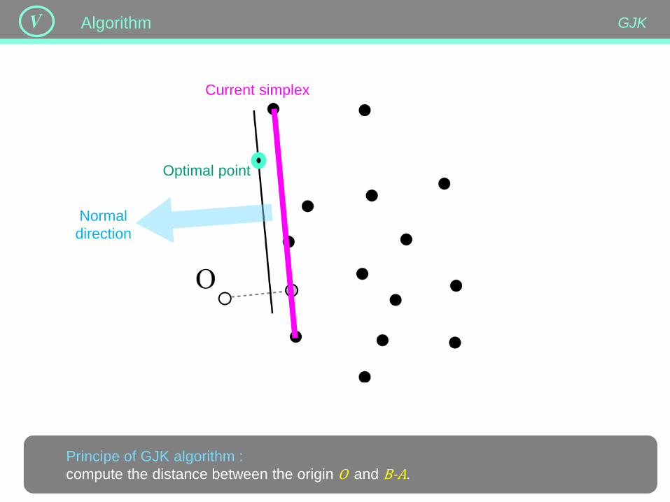
Principe of GJK algorithm :
compute the distance between the origin O and B-A.
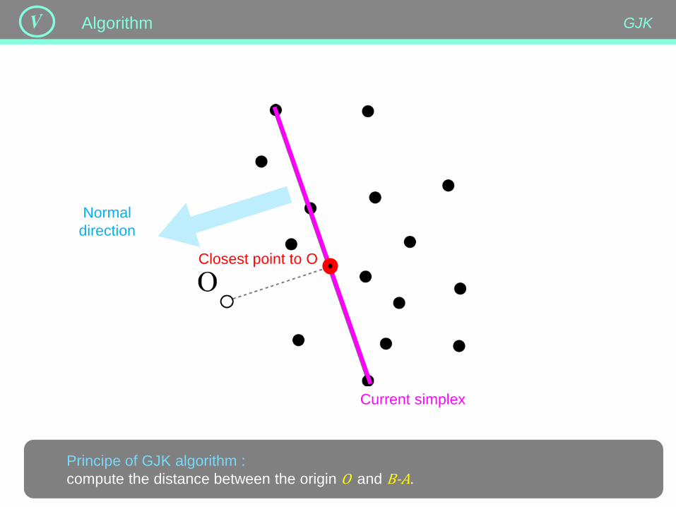
Current simplex
GJK Algorithm
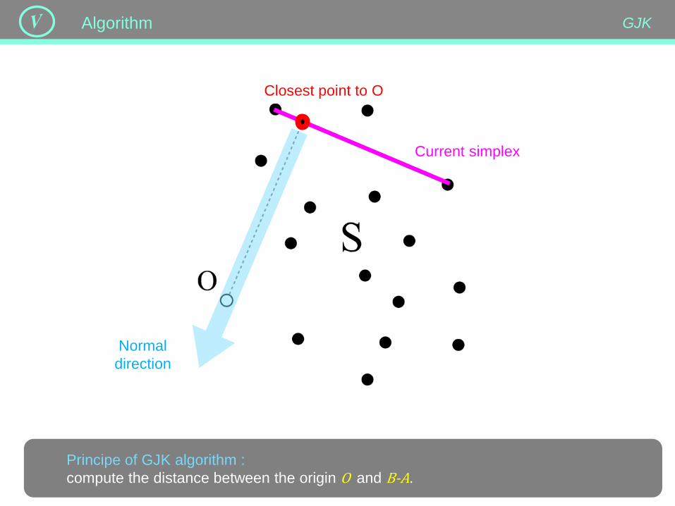
Principe of GJK algorithm :
compute the distance between the origin O and B-A.
Current simplex
Closest point to O
Normal
direction
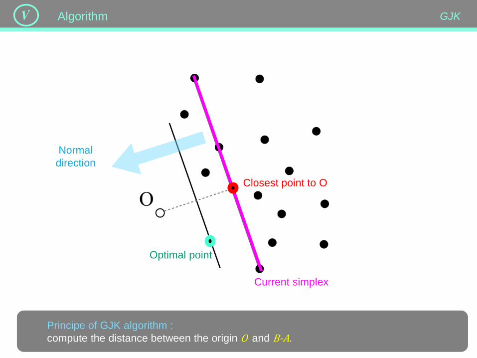
GJK Algorithm

Principe of GJK algorithm :
compute the distance between the origin O and B-A.
Current simplex
Closest point to O
Normal
direction Optimal point
GJK Algorithm

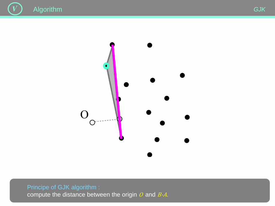
Principe of GJK algorithm :
compute the distance between the origin O and B-A.
Optimal point
GJK Algorithm
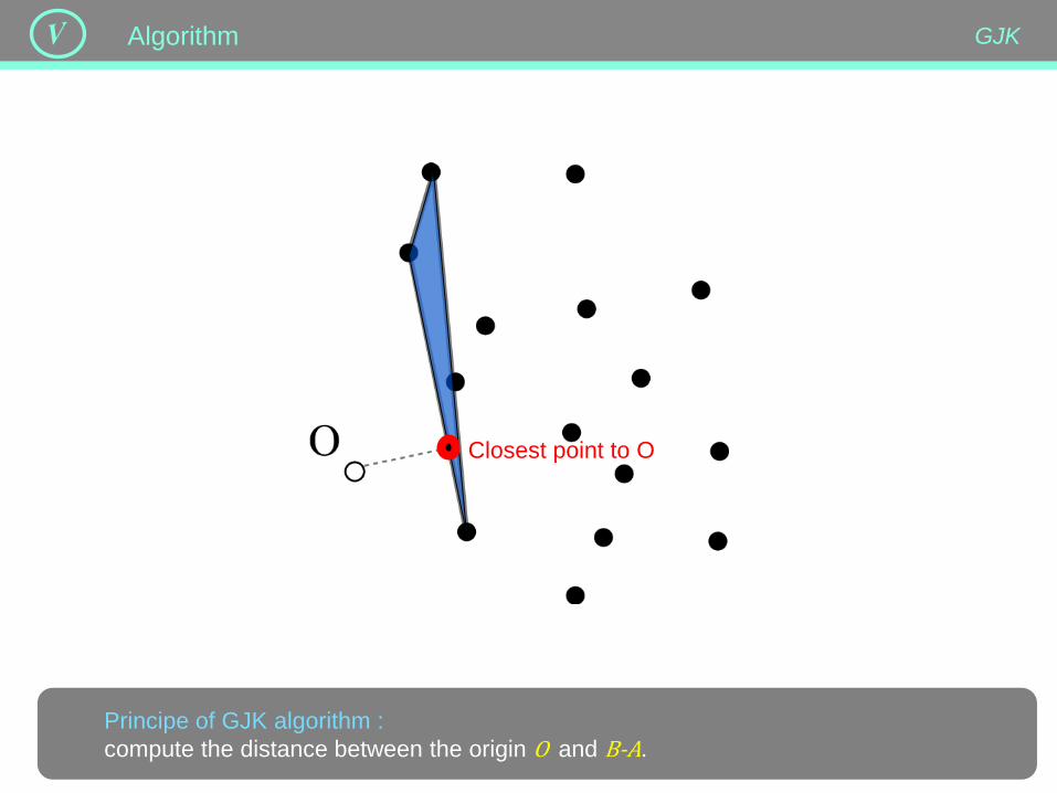
Principe of GJK algorithm :
compute the distance between the origin O and B-A.
Closest point to O
GJK Algorithm
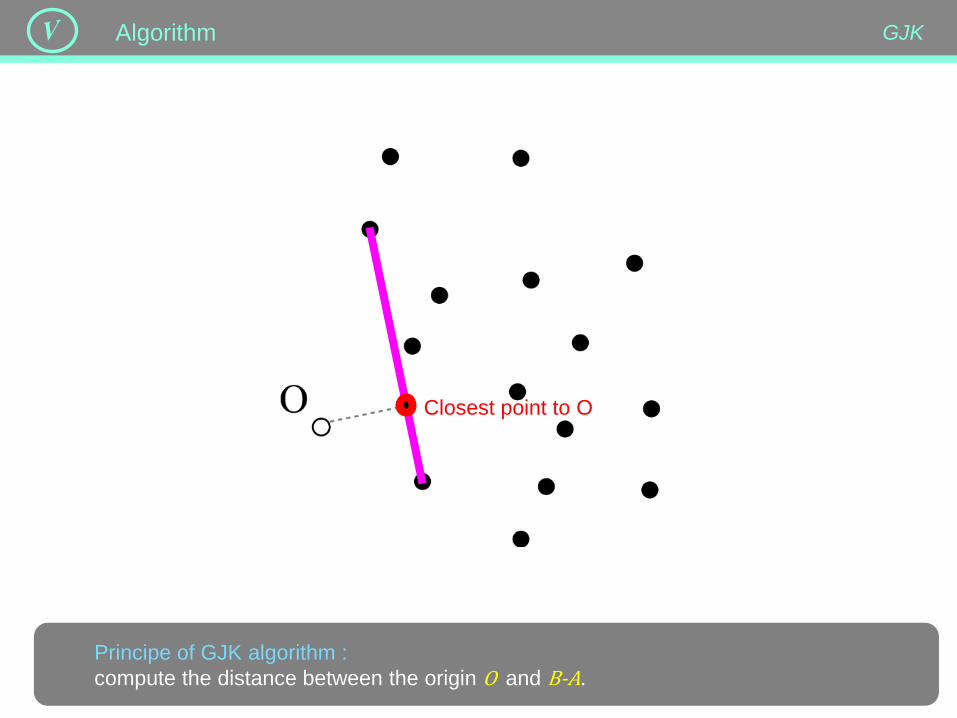
Principe of GJK algorithm :
compute the distance between the origin O and B-A.
Current simplex
Closest point to O
Normal
direction
GJK Algorithm
Principe of GJK algorithm :
compute the distance between the origin O and B-A.
Current simplex
Normal
direction
Optimal point
Closest point to O
GJK Algorithm

Principe of GJK algorithm :
compute the distance between the origin O and B-A.
Optimal point
GJK Algorithm

Principe of GJK algorithm :
compute the distance between the origin O and B-A.
Closest point to O
GJK Algorithm
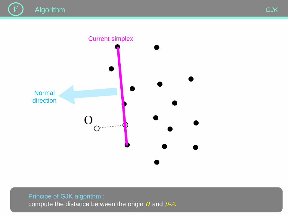
Principe of GJK algorithm :
compute the distance between the origin O and B-A.
Current simplex
Normal
direction
GJK Algorithm
Principe of GJK algorithm :
compute the distance between the origin O and B-A.
Current simplex
Normal
direction
Optimal point
GJK Algorithm
Principe of GJK algorithm :
compute the distance between the origin O and B-A.
GJK Algorithm
Principe of GJK algorithm :
compute the distance between the origin O and B-A.
Closest point to O
GJK Algorithm
Principe of GJK algorithm :
compute the distance between the origin O and B-A.
Closest point to O
GJK Algorithm
Conclusion
115
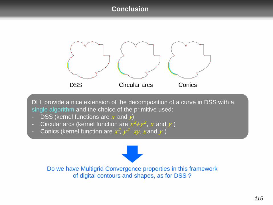
DLL provide a nice extension of the decomposition of a curve in DSS with a
single algorithm and the choice of the primitive used:
- DSS (kernel functions are x and y)
- Circular arcs (kernel function are x²+y² , x and y ) - Conics (kernel function are x², y² , xy, x and y )
DSS Circular arcs Conics
Do we have Multigrid Convergence properties in this framework of digital contours and shapes, as for DSS ?

Further works
116
DLL works also in 3D and more:
Provide also multigrid convergence results…
It’s time consuming to compute the derivatives all along a curve :
Provide an enhanced version
with point deletion and insertion…