Embed Size (px)
Citation preview
Digital Topology
Ulrich EckhardtDepartment of Applied Mathematics
University of HamburgBundesstraße 55
D–20 146 Hamburg, Germany
and
Longin LateckiDepartment of Computer Science
University of HamburgVogt–Kolln–Straße 30D–22 527 Hamburg
February 26, 2008
To appear in Trends in Pattern Recognition,Council of Scientific Information, Vilayil Gardens, Trivandrum, India.
Hamburger Beitrage zur Angewandten MathematikReihe A, Preprint 89
October 1994
Contents
1 Introduction 11.1 Motivation and Scope . . . . . . . . . . . . . . . . . . . . . . . . . . . . . . . . . . . . . . . . 11.2 Historical Remarks . . . . . . . . . . . . . . . . . . . . . . . . . . . . . . . . . . . . . . . . . . 3
2 The Digital Plane 32.1 Basic Definitions . . . . . . . . . . . . . . . . . . . . . . . . . . . . . . . . . . . . . . . . . . . 32.2 Jordan’s Curve Theorem . . . . . . . . . . . . . . . . . . . . . . . . . . . . . . . . . . . . . . . 42.3 The graphs of 4– and 8–topologies . . . . . . . . . . . . . . . . . . . . . . . . . . . . . . . . . 6
3 Embedding the Digital Plane 73.1 Line Complexes . . . . . . . . . . . . . . . . . . . . . . . . . . . . . . . . . . . . . . . . . . . . 73.2 Cellular Topology . . . . . . . . . . . . . . . . . . . . . . . . . . . . . . . . . . . . . . . . . . . 11
4 Axiomatic Digital Topology 124.1 Definition and Simple Properties . . . . . . . . . . . . . . . . . . . . . . . . . . . . . . . . . . 124.2 Connectedness . . . . . . . . . . . . . . . . . . . . . . . . . . . . . . . . . . . . . . . . . . . . 144.3 Alexandroff Topologies for the Digital Plane . . . . . . . . . . . . . . . . . . . . . . . . . . . . 17
5 Semi–Topology 195.1 Motivation . . . . . . . . . . . . . . . . . . . . . . . . . . . . . . . . . . . . . . . . . . . . . . 195.2 The Associated Topological Space . . . . . . . . . . . . . . . . . . . . . . . . . . . . . . . . . 205.3 Related Concepts . . . . . . . . . . . . . . . . . . . . . . . . . . . . . . . . . . . . . . . . . . . 215.4 Connectedness . . . . . . . . . . . . . . . . . . . . . . . . . . . . . . . . . . . . . . . . . . . . 225.5 Ordered Sets . . . . . . . . . . . . . . . . . . . . . . . . . . . . . . . . . . . . . . . . . . . . . 23
6 Applications to Image Processing 246.1 Models for Discretization . . . . . . . . . . . . . . . . . . . . . . . . . . . . . . . . . . . . . . 246.2 Continuity . . . . . . . . . . . . . . . . . . . . . . . . . . . . . . . . . . . . . . . . . . . . . . . 246.3 Homotopy . . . . . . . . . . . . . . . . . . . . . . . . . . . . . . . . . . . . . . . . . . . . . . . 256.4 Fuzzy Topology . . . . . . . . . . . . . . . . . . . . . . . . . . . . . . . . . . . . . . . . . . . . 25

Abstract
The aim of this paper is to give an introduction intothe field of digital topology. This topic of researcharose in connection with image processing. It is im-portant also in all applications of artificial intelligencedealing with spatial structures.
In this article, a simple but representative modelof the Euclidean plane, called the digital plane, isstudied. The problem is to introduce a satisfactory‘topology’ for this essentially discrete structure. Itturns out, that all known approaches, which comefrom different directions of applications and theory,converge to virtually one concept of 4/8– or 8/4–connectedness.
A very natural approach to problems of discretetopology is the concept of semi–topological spaces.
1 Introduction
1.1 Motivation and Scope
The only sets which can be handled on computers arediscrete or digital sets, wich means sets that containat most a denumerable number of elements. Thereare two sources for discrete sets
• The data structures of computer science are enu-merable by definition. So, only discrete objectscan be represented. This covers a great numberof practical situations. For example in most ap-plications of Artificial Intelligence the universeof discourse is a finite set. Another example isdiscrete classification e.g. of plants and animalsor stars into spectral classes etc.
• Continuous objects are discretized, i.e. they areapproximated by discrete objects. This is donee.g. in finite element models in engineering butalso in image processing where the intrinsicallycontinuous image is represented by a discrete setof ‘pixels’.
In some cases the objects under consideration aretaken from a space with certain geometric charac-teristics. Any useful discrete model of the situa-tion should model the geometry faithfully in order
to avoid wrong conclusions. For example, if an au-tomatic reasoning system should interpret correctlythe sentence “The policemen encircled the house”, itmust be able to understand that it is not possible toleave the house without meeting a policeman. Math-ematically speaking, the set of policemen has somesort of ‘Jordan curve property’ which enables themto separate the house from the remainder of the worldunless one is able to act in three dimensions.
It is clear, that no discrete model can exhibit all rel-evant features of a continuous original. Therefore, onehas to accept compromises. The compromise chosendepends on the specific application and the questionswhich are typical for the application. Digital geome-try is an attempt to evaluate the price one has to payfor discretization. The most simple part of geometryis topology. The digital model topology necessarily re-flects only certain facets of the underlying continuousstructure. It is therefore necessary to apply differentapproaches to digital topology.
Our visual system seems to be well adapted to copewith topological properties of the world. For exam-ple, letters in a document can be classified in a firststep according to their topological homotopy types.The layout of documents frequently is based on topo-logical predicates (e.g., a specific item must appearwithin a preassigned box). Optical checking of wiringof chips amounts in finding out whether the wiringhas the homotopy type wanted.
There are mainly three approaches for defining adigital analog of the well–known ‘natural’ topologyof the Euclidean space:
Graph–Theoretic Approach A very elementarystructure which can be handled easily on com-puters is a graph. A graph is obtained when aneighborhood relation is introduced into the dig-ital set. Such a structure allows to investigateconnectivity of sets.
Imbedding Approach The discrete structure isimbedded into a known continuous structure,usually into an Euclidean space. Topologicalproperties of discrete objects are then definedby means of their continuous images.
Axiomatic Approach Certain subsets of the un-
1

derlying digital structure are declared to be‘open sets’ and are required to fulfill certain ax-ioms. These axioms have to be chosen in sucha way that the digital structure gets propertieswhich are as close as possible to the propertiesof usual topology.
All three approaches have advantages and disad-vantages. The axiomatic approach is mathematicallyvery elegant but it does not directly provide thelanguage which is wanted in applications. The ob-jects which are practically investigated are not opensets but rather connected sets, sets which are con-tained in other sets etc. The graph theoretic approachyields directly connectedness but is beomes very diffi-cult to handle more complicated concepts of topologysuch as continuity, homotopy etc. The embedding ap-proach is of course only adequate for structures whichcan be related to an Euclidean space. The problem isthat one has to find for each question an appropriateembedding.
There are many proposals in the literature whichdeal with topological questions. Of course, these pro-posals cannot always be characterized by only one ofthe approaches given above.
We list some of the questions which are typicallyattacked by digital topology:
• Definition of connectedness and connected com-ponents of a set.
• Classification of points in a digital set as interiorand boundary points, definition of boundaries ofdigital sets.
• Formulation of Jordan’s Curve Theorem (andits higher dimensional analogs). This theoremstates that a set can be represented by its bound-ary which leads to a reduction of dimensionalityin the representation. This Theorem is, as men-tioned above, essential for understanding spatialrelations and is used for grouping items in spatialdata structures.
• One very important topological ‘invariant’ of aset is its Euler number. This number is in a cer-tain sense all what we can get by parallel workingmachines.
• General topology deals mainly with continuousfunctions. Such functions have no counterpartsin discrete structures. However, it would be use-ful for many applications to have such a conceptas ‘discrete continuity’.
• By means of a suitable definition of continuityone is able to compare topological structureswith each other. A very powerful concept intopology is homeomorphy. Homeomorphic topo-logical structures are topologically the same. So,if a topological problem is investigated, one hasto look for a homeomorphic structure in whichthe problem can be stated and solved as easilyas possible.
• Homotopy theory deals with properties of setswhich are invariant under continuous deforma-tions. Translating homotopy from general topol-ogy to discrete structures raises a number ofquestions which are not yet solved in a satis-factory way. On the other hand, one of the mostoften used preprocessing methods in image pro-cessing is thinning which is the numerical real-ization of a ‘deformation retract’ from homotopytheory.
There are several practical situations other thanimage processing or spatial reasoning in artificialintelligence where topological spaces were used tomodel discrete situations, starting from Alexandrov’swork in 1935 (see [1, 2]). In these publications,Alexandroff provided a theoretical basis for the topol-ogy of ‘cell complexes’.
• In his book on the lambda calculus, Barendregtuses the Scott topology [10, p. 9 f.] for partiallyordered sets [55], [56]. By means of this topol-ogy, concepts such as continuity of functions canbe introduced. There exist numerous publica-tions on application of discrete topologies to datastructures, abstract computing models, combi-natorial algorithms, complexity theory and log-ics.
• By using a suitable topology over the attributeset, Baik and Miller attempted to test equiva-lence of heterogeneous relational databases [9].
2

• Brissaud [12, 13, 14] defined a so–called ‘pre–topology’ for modelling preference structures ineconomics. (for other applications in economicssee [4], [5], [6], [7]).
These pre–topological spaces were later used byArnaud et al. [8] in image processing.
In this paper, only topologies for the 2–dimensionalrectangular grid Z2 are considered. This grid can beunderstood to be the set of all points of the Euclideanplane R2 having integer coordinates. A more generaltheory is possible [52] but for easier presentation thisis not attempted here. The reader should be familiarwith elementary topology of the Euclidean plane.
For survey articles on digital topology the readeris referred to [26, 31, 35].
Points in the digital plane Z2 are indicated byupper–case letters, points in the Euclidean plane R2
by lower–case letters. Vectors are understood to becolumn vectors. For easier typographic representationwe often write P = (m,n)> for the vector P ∈ Z2
having integer coordinates m and n.For a finite set S we denote by |S| the number of
its elements. The notation A := B means that A isdefined by expression B.
1.2 Historical Remarks
In 1935 Alexandroff and Hopf published a textbookon topology [2]. In this book an axiomatic basis wasgiven for the theory of cell complexes (so–called com-binatorial topology). This theory was developed atthe begin of this century in order to attack very diffi-cult problems of topology. In 1937 Alexandroff pub-lished a paper on the same subject where the term“Discrete Topology” was explicitly used in the ti-tle [1]. E. Khalimsky investigated ordered connectedtopological spaces and wrote a book on this topicin 1977. Later on, in collaboration of the New Yorkschool of topology (Kopperman, Meyer, Kong andothers) it turned out that the ordered connectedspaces are very well suited for treating problems ofdigital topology. They are equivalent to Alexamndroffspaces. At the end of the eighties V. Kovalevsky gavea sound fundament for digital topology [36], whichagain turned out to be part of Alexandroff theory. A
similar theory was provided in the same time by G.Herman [23].
In 1979 A. Rosenfeld published a paper which hadthe title “Digital Topology” [53]. This paper was veryinfluential since for the first time some very difficultproblems of digital topology were treated rigorously.The paper was based on results of Duda, Hart andMunson [17].
2 The Digital Plane
2.1 Basic Definitions
As a simple but nevertheless useful model we considerthe digital plane Z2 which is the set of all points inthe plane R2 having integer coordinates.
Digital Topology and Geometry are concerned withtopological and geometrical properties of subsets ofthe digital plane, so–called digital sets. Digital Topol-ogy and Geometry are not new areas of mathematics.Many of the problems encountered in this connectionare familiar from geometry of numbers [47, 20], fromstochastic geometry [46, 57, 58, 59], integral geometry[11, 46] and from discretization of partial differentialequations [44].
In image processing the digital plane is taken as amathematical model of digitzed black–white images.In this application one usually has a given set, namelythe set S of black points in the image and the com-plement CS, which is the set of white points.
Given a point P = (m,n)> ∈ Z2. The 8–neighborsof P are all points with integer coordinates (k, `)>
such that
max (|m− k|, |n− `|) ≤ 1.
We number the 8–neighbors of P in the following way:
3

column
row n− 1 n n + 1
m + 1 N3(P ) N2(P ) N1(P )
m N4(P ) P N0(P )
m− 1 N5(P ) N6(P ) N7(P )
Neighbors with even number are the direct or 4–neighbors of P , those with odd numbers are the in-direct neighbors. The 8–neighborhood N8(P ) of P isthe set of all 8–neighbors of P (excluding P ), the 4–neighborhood N4(P ) of P is the set of all 4–neighborsof P .
Let κ be any of the numbers 4 or 8 and let I ={0, 1, · · · , n} be a (finite) interval of consecutive inte-gers. A digital κ–path or simply path P is a sequence{Pi}i∈I of points in Z2 such that Pi and Pj are κ–neighbors of each other whenever |i − j| = 1. Wenote that the order induced by the numbering of thepoints of a path is essential. For P ∈ P we define theκ–degree or degree of P with respect to P to be thenumber |P ∩Nκ(P )|. A point of P having degree 1 istermed an end point. It is an immediate consequenceof the definition that any point of a path has degreeat least one. There exist at most two end points in apath. End points can only correspond to numbers 0or n. A path with the property P0 = Pn is called aclosed path. A closed path contains no end points.
A κ–path P is termed a κ–arc or simply an arc ifit has the additional property that for any two pointsPi, Pj ∈ P which are not end points Pi ∈ Nκ(Pj) im-plies |i− j| ≤ 1. Consequently, an arc is a path whichdoes not intersect or touch itself with the possibleexception of its end points. Any point of an arc hasorder one or two.
We state a very simple but important Lemma:
Lemma 1 Let P be a path with two end points. Thenthere exists an arc P0 which is completely containedin P and has the same end points.
Proof If P is a κ–path but not a κ–arc then itcontains at least one pair of points Pi and Pk such
that Pi ∈ Nκ(Pk), but |i − k| > 1. Assume withoutloss of generality k > i. Then the path
P ′ := {P0, P1, · · · , Pi−1, Pi, Pk, Pk+1, · · · , Pn}
is contained in P, has end points P0 and Pn, buthas fewer elements as P. Repeating the procedure weeventually arrive at an arc with the desired property.2
A digital set S ⊆ Z2 is termed a κ–connected setwhenever for any two points P,Q ∈ S there exists apath P with the properties that it is completely con-tained in S and that it contains both P and Q. Dueto Lemma 1 we may in this definition replace ‘path’by ‘arc with end points P and Q’. A connected com-ponent of a set S ⊆ Z2 is a maximal subset of S whichis connected. This purely graph theoretic concept ofconnectedness is very fundamental for analyzing dig-ital sets. By means of connectedness we introducesome sort of rudimentary topology in Z2. We there-fore adopt here the familiar terminology of speakingabout 4– and 8–topology for the digital plane.
2.2 Jordan’s Curve Theorem
A very fundamental property — for theory as well asfor applications — of the topology of the plane is thatJordan’s Curve Theorem is valid. That means thatany “simple closed curve” has the property of sepa-rating the plane into two parts, namely the interiorwith respect to the curve and the exterior. These twoparts of the plane are distinguished by the fact thatthe latter is not bounded. For our purposes we onlyneed this theorem for polygonal curves. A polygonalcurve or simply curve in the plane consists of a fi-nite number of points {x0, x1, · · · , xn} called verticessuch that each two consecutive vertices xi, xi+1 arejoined by a line segment called an edge. A polygonalcurve is termed a simple (polygonal) curve if edgesmeet only in vertices and if for each vertex there areat most two edges meeting it. It is termed a closed(polygonal) curve if x0 = xn.
Since Z2 can be considered as a subset of R2, anypath in Z2 corresponds to a polygonal curve in theplane R2 with vertices in Z2 and every arc corre-sponds to a simple curve in the plane. Similarly, a
4

closed path (arc) corresponds to a closed polygonalcurve (simple curve).
Theorem 1 (Jordan’s Curve Theorem) Givena simple closed polygonal curve C in the plane R2.
Then R2 \ C consists of exactly two open connectedsets (in the sense of the ordinary R2–topology). Ex-actly one of these sets is bounded and is called theinterior with respect to C and the other one is un-bounded and is called the exterior with respect to C.
The proof of this Theorem is quite elementary butsomewhat lengthy. We refer the reader to the litera-ture (a very simple proof can be found in [3, ChapterI, §7.9]).
The ‘digital analog’ of this fundamental Theoremcan be naively formulated in the following way:
Given a closed simple curve P in the digitalplane Z2.Then Z2 \ P consists of exactly two con-nected sets. Exactly one of these sets isbounded and is called the interior with re-spect to P and the other is unbounded andis called the exterior with respect to P.
If we interpret the term ‘curve’ as ‘arc’ then the as-sertion of the Theorem as formulated here is not true.The following two sets are closed arcs in the sense ofthe definition above but the complement (with re-spect to Z2) of each of them consists of only one con-nected component. Arrows in the figures indicate theorder imposed by numbering the points.
8–connectivity: s ss- 6��
4–connectivity: s sss- 6
�
?
In order to rule out such singularities, we explic-itly require that a closed digital 8–curve must have
at least four points and a closed digital 4–curve musthave at least eight points. Since there exist (up totranslations, rotations by multiples of 90o and re-flections at diagonal lines of the digital plane) onlyfinitely many arcs having fewer than four or eightpoints, respectively, the reader can easily verify byinspecting all possible cases that this restriction in-deed makes sense. In the following, a digital curve isunderstood to be an arc which fulfills the restrictionmentioned above if it is closed.
There is, however, a second problem. Consider thetwo following digital sets (black points (•) are under-stood to belong to S, white points (◦) to the comple-ment):
c c c c c
c c c c c
ccc
ccc
s sss cc cc c@@R ���
@@I��
c c c c c c
c c c c c c
cccc
cccc
s s s
s s sss s s ssc cc
c- - 6
- 6
6
��
?�
?
?
The first set is an 8–curve (in the 4–sense it is not acurve). Its complement, however, consists of only one8–connected component. Similarly the second set isa 4–curve (but not an 8–curve) and its complementconsists of three 4–components. These phenomenaare sometimes called ‘connectivity paradoxa’.
In 1979 Rosenfeld [53] proved that Jordan’s curveTheorem is indeed true for digital curves if thecurve and its complement are equipped with differ-ent ‘topologies’. This was observed earlier by Duda,
5
Hart and Munson [17]. Rosenfeld was the first to givethese results a sound theoretical background.
We define for κ ∈ {4, 8}
κ :={
4 for κ =88 for κ =4.
(1)
The following Theorem holds:
Theorem 2 (Digital Jordan Theorem) Given aclosed simple κ–curve P in the digital plane Z2.
Then Z2 \ P consists of exactly two κ–connectedsets. Exactly one of these sets is bounded and is calledthe interior with respect to P and the other is un-bounded and is called the exterior with respect to P.
Rosenfeld’s proof of this Theorem is performed es-sentially by an embedding approach. We return tothis subject later on.
In image processing applications the sets of blackpoints are considered to carry the essential informa-tion of a black–white image. Therefore usually the setof all black points is equipped with the 8–topologysince this topology exhibits a more complex connec-tivity structure. We will follow this custom here andalso use the 8–topology. It is easily possible to obtainassertions about the 4–topology by investigating thenegative image which is obtained by changing theroles of S and its complement. This has to be car-ried out with some caution since the situation is notquite symmetric because we sometimes assume S tobe bounded.
Digital curves play a special role in image process-ing applications. First it is possible to represent digi-tal curves in a storage efficient way by storing the co-ordinates of P0 and then only the differences Pi+1−Pi
for i = 0, 1, · · · , n−1. These differences can be codedby storing only the number in the neighborhood con-figuration of Pi which corresponds to Pi+1. This codefor a digital path is named chain code. For codingeight neighbors of a point one needs 3 bits, hence acurve of length n can be stored using 3n bits if oneneglects the amount of storage necessary to store thefirst point P0.
For storing binary images it is sufficient to codeonly the boundaries of the black digital sets. The jus-tification of representing a digital set by its bound-ary is given by Jordan’s Curve Theorem. A binary
image consisting of n × n points can be stored us-ing n × n bits. If only the boundaries of the blacksets are stored, one needs 3nB bits, where nB is thenumber of boundary points. Coding the boundariespays when the number of boundary points is less than33 % of the total number of points in the image. Inusual text documents the number of boundary pointsamounts to less than 10 % of the number of all points,and this figure is even smaller in line-structured im-ages such as engineering drawings. With growing res-olution of scanners the number of boundary pointsgrows roughly linear with the number of discretiza-tion points per unit length, the total number of im-age points (as well as the number of black points),however, grows as the square of the number of dis-cretization points per unit length. As a consequence,boundary coding of images becomes more and moreattractive with growing resolution power of scanningdevices.
2.3 The graphs of 4– and 8–topologies
The approach presented in this section to ‘topologize’the digital plane is mainly based on graph theoreticideas. It uses concepts such as points of Z2 being thenodes of the graph, and a neigborhood relation whichis represented by the edges of the (undirected) graph.This model enabeled us to speak about connectivityof sets in a graph theoretic manner. The graphs repre-senting 4– and 8–connectivity are depicted in Figure1.
The graph corresponding to the 4–topology is pla-nar, which means that it can be drawn in the planesuch that the lines representing the neighborhood re-lation meet only in vertices. In contrast, it is not pos-sible to represent the connectivity of 8–topology bymeans of a planar graph. This implies that the no-tions “planarity” and “topology of the digital plane”are not equivalent.
In order to prove that the 8–topology cannot bemodelled by a planar graph we show that the Kura-towski graph K5 can be drawn into the graph of thedigital plane equipped with the 8–topology. Accord-ing to Kuratowski’s theorem, a graph is not planar ifand only if it has a subgraph homeomorphic to K5
or K3,3 (see [22, Theorem 11.13]). K5 is the com-
6

cc
cccc
cccc
cccc
cccc
ccc
ccccc
cccc
cccc
cccc
ccc
ccccc
cccc
cccc
cccc
ccc
ccccc
cccc
cccc
cccc
ccc
ccccc
cccc
cccc
cccc
cc
cc
cc
��
��@@
@@
��
@@
@@
��
cc
cc
��
��@@
@@
��
@@
@@
��
cc
cc
��
��@@
@@
��
@@
@@
��
cc
cc
��
��@@
@@
��
@@
@@
��
cc
cc
��
��@@
@@
��
@@
@@
��cc
cc
��
��@@
@@
��
@@
@@
��
cc
cc
��
��@@
@@
��
@@
@@
��
cc
cc
��
��@@
@@
��
@@
@@
��
cc
cc
��
��@@
@@
��
@@
@@
��
cc
cc
��
��@@
@@
��
@@
@@
��cc
cc
��
��@@
@@
��
@@
@@
��
cc
cc
��
��@@
@@
��
@@
@@
��
cc
cc
��
��@@
@@
��
@@
@@
��
cc
cc
��
��@@
@@
��
@@
@@
��
cc
cc
��
��@@
@@
��
@@
@@
��cc
cc
��
��@@
@@
��
@@
@@
��
cc
cc
��
��@@
@@
��
@@
@@
��
cc
cc
��
��@@
@@
��
@@
@@
��
cc
cc
��
��@@
@@
��
@@
@@
��
cc
cc
��
��@@
@@
��
@@
@@
��cc
cc
��
��@@
@@
��
@@
@@
��
cc
cc
��
��@@
@@
��
@@
@@
��
cc
cc
��
��@@
@@
��
@@
@@
��
cc
cc
��
��@@
@@
��
@@
@@
��
cc
cc
��
��@@
@@
��
@@
@@
��
Figure 1: Graphs corresponding to the 4–topology (left) and 8–topology (right). Circles (◦) denote gridpoints, lines indicate the appropriate neighbor relations.
plete graph having 5 nodes. In Figure 2 it is shownhow to embed K5 homeomorphically into the graphcorresponding to the 8–topology.
3 Embedding the Digital Plane
The digital plane Z2 can be considered as a subsetof R2. This leads immediately to the embedding ap-proach for digital topology. We only sketch here twomodels for illustration purposes (see also [29, 33]).
3.1 Line Complexes
A line complex in the Euclidean plane consists of afinite number of points, termed vertices. Certain ofthe vertices are connected together by line segments,the edges. We assume that any two edges meet atmost in a vertex and that any vertex belongs to atleast one edge. The two points connected by an edgeare termed the end points of this edge. A vertex istermed incident to an edge if it is an end point ofthe edge. In an analogous way, two edges are termedincident if both are incident to a common vertex. The
polygonal curves introduced in section 2 are examplesfor line complexes. The concept of a line complex canbe easily generalized to higher dimensions. On linecomplexes we may define in a ‘naive’ way topologicalconcepts such as paths, arcs and connectivity. More-over, since we only consider line complexes which areembedded into an Euclidean space Rd, we can usethe known topology of Rd for investigating topolog-ical properties of the complement of a line complexwith respect to Rd. So, a subset of the complementis termed connected whenever any two points of thisset can be joined by a curve which is completely con-tained in the set. In the context of line complexes itis sufficient to consider only polygonal curves.
Given a digital set S and κ ∈ {4, 8}, κ ∈ {4, 8} \{κ} (see (1)). For each κ–connected component of Sand each κ–connected component of the complement(with respect to Z2) of S we construct a line complexwhich will be called the line complex associated toS (or the complement of S, respectively). This linecomplex has the points of S (or of the complementof S, respectively) as vertices. If S is equipped withthe 4–topology, any two directly neighboring points
7

s s
ss
s
...............................................................................................................................................................................................................................
....................................................
....................................................
....................................................
....................................................
.................
.....................................................................................................................................................................................................................................................................................
...........................................................................................................................................................................
...........................................................................................................................................................................
.....................................................................................................................................................................................................................................................................................
....................................................
....................................................
....................................................
....................................................
....................................................
................. ....................................................
....................................................
....................................................
...............
.....................................................................................................................................................................................................................................................................................
...........................................................................................................................................................................
cccccc
cccccc
cccccc
cccccc
cccccc
s s ss s@
@@@ �
���
��
��@@
@@ ��
��
��
�� @@
@@
Figure 2: Homeomorphic embedding of the Kuratowski graph K5 (left) into the digital plane equipped withthe 8–topology (right). The nodes of the embedded graph K5 are marked ‘•’.
in S will be joined by an edge. If S is equipped withthe 8–topology, also indirectly neighboring points inS will be joined by a diagonal edge. In order to makethis construction consistent with the definition of aline complex, we introduce extra vertices whenevertwo diagonal edges meet. Analogously we define forthe complement of S.
One easily shows:
Theorem 3 The line complexes belonging to S andto the complement of S are disjoint.
Proof We assume that each vertex of the digitalplane has color black if it belongs to S and color whiteotherwise. It is clear that the sets of vertices of bothline complexes are disjoint.
By definition of the associated line complex, whenan edge joins two points of the digital plane, thesepoints have the same color. In this case we associateto the edge the color of its end points.
There remain the extra vertices and the edges join-ing points in Z2 with an extra vertex. However, an
extra vertex is only introduced if it is on a diagonalline joining two points of the same color which are in-direct neighbors of each other. Consequently, we canuniquely associate a color to each extra vertex andalso to an edge joining a point in Z2 with an extravertex. 2
Remark 1 The meaning of the last Theorem is il-lustrated by the following configuration:
s csc��
If the set of black points (•) is equipped with the8–topology, then the two black points in the pictureare connected by an edge. Then, however, it is nolonger possible to join both white points (◦) also byan edge since both edges would intersect and thus itwould be no longer possible to assign them a color inan unambiguous way.
8

Theorem 4 1. A digital set is connected if and onlyif the line complex associated to it is connected.
2. The line complex associated to a digital set hasthe same number of connected components as the dig-ital set itself.
3. A digital set is a digital path (a closed digitalpath, a digital arc, a closed digital arc, respectively)if and only if the line complex associated to it is apolygonal path (a closed polygonal path, a polygonalcurve, a closed polygonal curve, respectively).
The proof of this theorem is not difficult and is leftto the reader. In performing the proof of Theorem4 it becomes clear why self–contacts are not allowedfor digital curves. When a digital curve touches it-self in two points which are not subsequent points,these points are ‘short-cut’ in the corresponding linecomplex, thus leading to an associated polygonal setwhich is not a polygonal curve.
The reason for dealing with associated line com-plexes is that much is known about the topology ofthem. Line complexes (and cell complexes) are well–known objects of combinatorial topology. So we caneasily reduce the proof of the Digital Jordan’s CurveTheorem 2 to that of Jordan’s Theorem 1 for polygo-nal curves. When a closed digital curve is given, thenthe line complex associated to it is a closed polyg-onal curve by Theorem 4, part 3. Since we explic-itly ruled out arcs containing no points of the dig-ital plane in the interior, the (digital) interior andthe exterior with respect to this polygonal curve arenot empty. By Theorem 4, part 2 both the interiorand the exterior are connected digital sets. As eachpoint in Z2 either belongs to the digital curve or toits complement, the Digital Jordan’s Curve Theoremis proved.
Similarly, assertions concerning Euler’s Theoremcan be derived for digital sets by using the corre-sponding theorems for line complexes. Euler’s Theo-rem gives a relation between the number of connectedcomponents of a polygonal set and the number of con-nected components of the complement of it.
Theorem 5 (Euler’s Theorem) For a line com-plex C in the plane denote by
v the number of vertices,
e the number of edges,r the number of connected components (in the nat-
ural topology of the plane) of the complement of C.Such components are called regions defined by C.
c the number of connected components of C.Then Euler’s relation holds:
v − e = c− r + 1.
The number E(C) := c − r + 1 is the Euler number(or genus) of the line complex C.
The proof of this Theorem is quite elementary. De-tails concerning this proof and also properties of linecomplexes in the plane and of cell complexes in threedimensions can be found in the book of Alexandrow[3, Chapter I, §7].
Euler’s theorem states that Euler’s number, whichcharacterizes a global topological property of C, canbe determined by counting (locally) numbers of ver-tices and edges. Such locally calculable propertiescan be determined by means of a very simple modelfor parallel computation. We assume that a proces-sor is located at each vertex. Each of the processorshas only information about the neighborhood of itsvertex. The processors are allowed to send messagesof limited information content to a master proces-sor which evaluates the information to find Euler’snumber. By means of such a model we can easily de-termine Euler’s number for a cell complex. There aretheoretical results showing that Euler’s number is theonly topological predicate of a cell complex which candetermined in such a way [48, 43, 30].
Assume that a digital set S is equipped with the 4–topology. Euler’s relation is true for the line complexassociated to the set with v denoting the number ofpoints in S and e the number of horizontal and ver-tical edges. In order to determine the number of re-gions we have to bear in mind that the associated linecomplex is a subset of the Euclidean plane R2. Theregions determined by the line complex are the opensets which constitute the complement of the line com-plex with respect to the plane. For sake of clarity wedenote the complement of a set S with respect to theEuclidean plane with CES := R2 \S. If S is a digitalset, its complement with respect to the digital plane
9

will be denoted CDS := Z2 \ S. There are two differ-ent types of such regions. The members of the firsttype are components of the complement of the linecomplex which do not contain any grid points belong-ing to CES (note that grid points in CES are pointsin CDS). These components are exactly the squaresencircled by trivial closed 4–curves of the form
s sss
We denote the number of these squares by s.The second type of connected components of the
complement consists of components containing atleast one grid point in CES. The set of points ofCDS contained in such a component is 8–connected.Assume that two points in CES can be joined by a(polygonal) curve which does not meet the line com-plex associated to S. If this curve meets a horizontalor vertical line joining two directly neighboring gridpoints, then at least one of these points belongs toCDS. From this observation we conclude that thenumber of regions which contain at least one gridpoint is equal to the number of connected compo-nents of the line complex associated to CDS and isalso equal to the number of 8–components of CDS.We denote this number by r8.
Euler’s Formula (Theorem 5) now yields
E4/8(S) := c4 − r8 + 1 = v − e + s.
where c4 is the number of 4–components of S. TheEuler number c4 − r8 + 1 is the number of 4–components of S minus the number of holes in S. Ahole is a bounded connected component of the com-plement of S (with respect to Z2).
The procedure is analogous in the case of the 8–topology: The number of vertices v is the number ofpoints in S. The number of edges is the sum of thenumber e of horizontal and vertical edges in S andthe sum d of all diagonal edges in S.
In order to calculate the number of regions definedby the line complex associated to S, we again distin-guish two types of regions. The first type consists of
regions containing no points from the complement ofS. It consists of triangles
s ss��
(and all triangles obtained by 90o–rotations there-from) and squares as above. Let t be the number oftriangles and s be the number of squares. For thelatter we observe that each square contains four tri-angles:
s ss s��@@ = s ss c�� + s cs s@@ +
+ s sc s�� + c ss s@@
In the center of the square there is a crossing pointof two lines which yields an extra vertex. Hence thereare s new vertices generated, 2s new edges (each di-agonal edge was already counted to yield the numberd and is now split into two half–edges) and 4s newregions out of s squares. For each square, the fourtriangles contained in it are already counted in thenumber of regions. Analogously as above, we add thenumber r4 of the 4–components of the complementCES corresponding to regions of second type.
We get
Total number of vertices: v + sTotal number of edges: e + d + 2sTotal number of regions: c4 + t.
Euler’s formula yields:
E8/4(S) := c8 − r4 + 1 = v − e− d + t− s.
From the formulae for E4/8 and E8/4 we concludethat Euler’s number of a digital set can be calculatedby (parallel) inspection of all 2× 2 neighborhoods if
10

different topologies are used for the digital set and forits complement. The latter requirement is essential,otherwise this assertion is not true [30]. It is an inter-esting fact that it can be made true also in this caseif a simple additional condition (well–composedness)is imposed on the sets under consideration [38].
Line complexes may also be used for classifying thepoints of a digital set S into interior and boundarypoints. An edge of the line complex associated to Sseparates two regions. If both regions are of the firsttype as defined above (i.e. they contain no points ofthe complement CDS of S), the edge is called an in-terior edge. Otherwise it is adjacent to at least one re-gion of second type. In this case it is termed a bound-ary edge. A point which is incident to a boundaryedge is termed a boundary point and all boundarypoints and boundary edges constitute the boundaryof S. A point in S which is not a boundary point istermed an interior point of S. Using these concepts,we can define boundaries of digital sets as orientedcurve–like sets.
It is possible to generalize the approach presentedhere to three and more dimensions [34, 41, 42].
3.2 Cellular Topology
Sometimes a different model for the digital plane isused, the so–called cellular model. This model wasintroduced by Alexandroff and Hopf [2, Erster Teil,erstes Kapitel, §1.1, Beispiel 4o] (see Figure 3).
s s s ss s s ss s s s
c c cc c c
Figure 3: The cellular model. To each point (•) in thedigital plane one square, four edges and four verticesare associated.
Given a digital set S ⊆ Z2, we associate to it a setof certain objects in the Euclidean plane R2. The firsttype of objects are squares which are considered tobe open in the R2–topology and are centered arounda grid point. If P = (m,n)> is a grid point in Z2,then the square corresponding to P is
π(P ) = πmn :={
(ξ, η)> ∈ R2∣∣∣
m− 12
< ξ < m +12, and
n− 12
< η < n +12
}.
Furthermore we have edges which are sides ofsquares (without the end points) and vertices whichare the vertices of squares. The topological closureπmn of square πmn consists of the square πmn to-gether with its vertices and edges. It is sometimescalled the pixel belonging to P = (m,n)>.
Of course, each (open) square whose center pointis in S should belong to the model of a given digitalset S. In order to get in the model connectedness, weare forced to associate also edges and vertices to themodel set of a digital set. We consider two differentsuch models:
The closed model C(S) is the union of all pixels (=closed squares) whose center point is in S.
In the open model O(S), all (open) squares withcenter point in S belong to O(S). Moreover, an edgebelongs to O(S) whenever it is boundary edge of twoadjacent squares belonging to O(S) and a vertex be-longs to O(S) if all edges incident to it belong toO(S).
We can then state the following Theorem:
Theorem 61.
O(S) = CEC(CDS),C(S) = CEO(CDS).
2. O(S) is open and C(S) is closed in the R2–topology.
3. The number of connected components of O(S)(in the R2–topology) is equal to the number of 4–components of the digital set S.
11

The number of connected components of C(S) isequal to the number of 8–components of S.
Proof 1. Assume that there is an x ∈ R2 whichbelongs to both O(S) and C(CDS). Then there existsa Q ∈ CDS such that x ∈ π(Q). Since π(P )∩ π(Q) =∅ for P 6= Q, x does not belong to any π(P ) with P ∈S. Similarly, it is clear that x cannot be on an edge ofO(S) since in this case both squares adjacent to thisedge must belong to points in S which contradicts x ∈π(Q). An analogous argument shows that x is not avertex. Therefore we conclude that C(S)∩O(CDS) =∅.
Assume now that there is an x ∈ R2 which belongsneither to O(S) nor to C(S). Then x is not containedin any π(P ) since every P ∈ Z2 either belongs to S orto CDS. Similarly, x cannot belong to an edge for ei-ther both adjacent squares belong to points in S thenthe edge belongs to O(S) or else one of these squaresbelongs to a point in CDS which implies x ∈ C(CDS).A similar argument holds for vertices which provesthe first assertion. The second assertion is proved inan analogous manner.
2. Given a sequence {xn} of points in C(S) converg-ing to a point x∗. Then we can find a finite numberof squares π(P ) ⊆ C(S) containing all xn. The unionof these squares is closed, hence x∗ ∈ C(S).
The assertion concerning O(S) follows by applica-tion of part 1.
3. If P and Q are 8–neighbors in Z2 then the linesegment joining P and Q is completely contained inC({P,Q}) which yields the first assertion. An anlo-gous argument leads to the second assertion. 2
One might ask why we need different continuousmodels for the digital plane. The reason is that it isnot possible to find a model which exhibits all topo-logical properties needed. This is due to the obviousfact that the digital plane has a structure which issignificantly different from that of the real plane. Forexample, in Z2 every bounded set is finite which isnot true for the real plane. Therefore it is necessaryto ‘tailor’ a continuous model for each specific inves-tigation of the digital plane.
4 Axiomatic Digital Topology
4.1 Definition and Simple Properties
A topological space consists of a set X of points suchthat certain subsets of X which are called open setsfulfill the properties (see [25])
TO1 X and ∅ are open,
TO2 The union of any family of open sets is open,
TO3 The intersection of any finite family of opensets is open.
The system of all open sets is termed the topology ofX and is denoted T .
An open set which contains a point of X is calleda neighborhood of this point.
There are two trivial topologies for a set X whichplay a role in the sequel. In the discrete topology Td
(in the strict sense) all subsets of X are declared tobe open and in the indiscrete topology Ti the onlyopen sets are the empty set and the whole space X.
A set S ⊆ X is called a closed set if its complementis open.
The following classification of topological spacesaccording to their separation properties is due to Kol-mogoroff (see [2] or [25]):
T0 For any two different points in X at least onehas a neighborhood not containing the other.
T1 For any two different points P and Q in X thereexists a neighborhood of P not containing Q anda neigborhood of Q not containing P .
T2 For any two different points P and Q in X thereexists a neighborhood of P and a neigborhoodof Q which are disjoint.
T2–spaces are termed Hausdorff spaces.
A topological space is termed discrete if the follow-ing is true:
TO3’ The intersection of any family of open sets isopen.
12

This notion is due to Alexandroff [1]. For a T1– orT2–space the discrete topology as defined here coin-cides with the discrete topology in the strict sense.For T0–spaces we must distinguish between the dis-crete topology in the strict sense and the discretetopology in the general sense. A discrete T0–space istherefore termed an Alexandroff space. Axiom TO3’can also be stated using closed sets: The union of anyfamily of closed sets is closed. In this formulation itbecomes clear that Alexandroff spaces are completelysymmetric with respect to open and closed sets.
In an Alexandroff space there exists for each pointP a smallest neighborhood of P which is open:
OP =⋂
P∈UUopen
U.
Because of the symmetry of Alexandroff spaces therealso exists a smallest closed set containing P :
CP =⋂
P∈VV closed
V.
A point P with CP = {P} is called a vertex point.
Theorem 71. For any two different elements P and Q of an
Alexandroff space is
P ∈ OQ =⇒ Q /∈ OP andP ∈ CQ =⇒ Q /∈ CP.
2. P ∈ CQ ⇐⇒ Q ∈ OP .3. CP ⊆ CQ ⇐⇒ OQ ⊆ OP.
Proof 1. The first assertion is an immediate con-sequence of the T0–property. For the second asser-tion assume without loss of generality that Q ∈ OP .Then, by virtue of the the first assertion, P ∈ COQ.Hence COQ is a closed set which contains P but notQ, consequently Q /∈ CP . This means that not bothQ ∈ CP and P ∈ CQ are possible.
2. Q /∈ OP means Q ∈ COP . However, COP isclosed and does not contain P , hence P /∈ CQ.
Similarly, P /∈ CQ implies Q /∈ OP .
3. COP is closed. Q /∈ OP means Q ∈ COP , henceP ∈ CP ⊇ CQ ⊆ COP which is not possible. Conse-quently, Q ∈ OP . If P 6= Q then Q /∈ CP by 1. CCPis open and contains Q, but not P . Therefore
OQ ⊆ OP ∩ CCP ⊆ OP.
2
A topological space X is termed locally finite if eachpoint P in X has a finite neighborhood and a finiteclosed set containing P .
Theorem 8 Let X be a locally finite Alexandroffspace. Then
1. Each set CP contains at least one vertex point.2. If CP 6= CQ, then there is a vertex point in one
of these sets which is not contained in the other set.
Proof 1. If CP = {P} then P is a vertex point.Otherwise there is a Q ∈ CP with Q 6= P . ThenP /∈ CQ ⊆ CP and CQ has fewer points than CP .Repeating the process with CQ we eventually arriveat a vertex point contained in CP .
2. If both sets are disjoint then the assertion followsfrom part 1. Otherwise CP ∩ CQ 6= ∅ and we canapply the construction of part 1 to find a vertex pointhaving the desired property. 2
The Theorem states that the mapping which as-signs to an element P in a locally finite Alexandroffspace the set of all vertex points in CP is injective.If this mapping is bijective, the space is termed acomplete space.
Example 1 As an example we consider a space Xconsisting of nine points
α, β, γ, δ; a, b, c, d;Q.
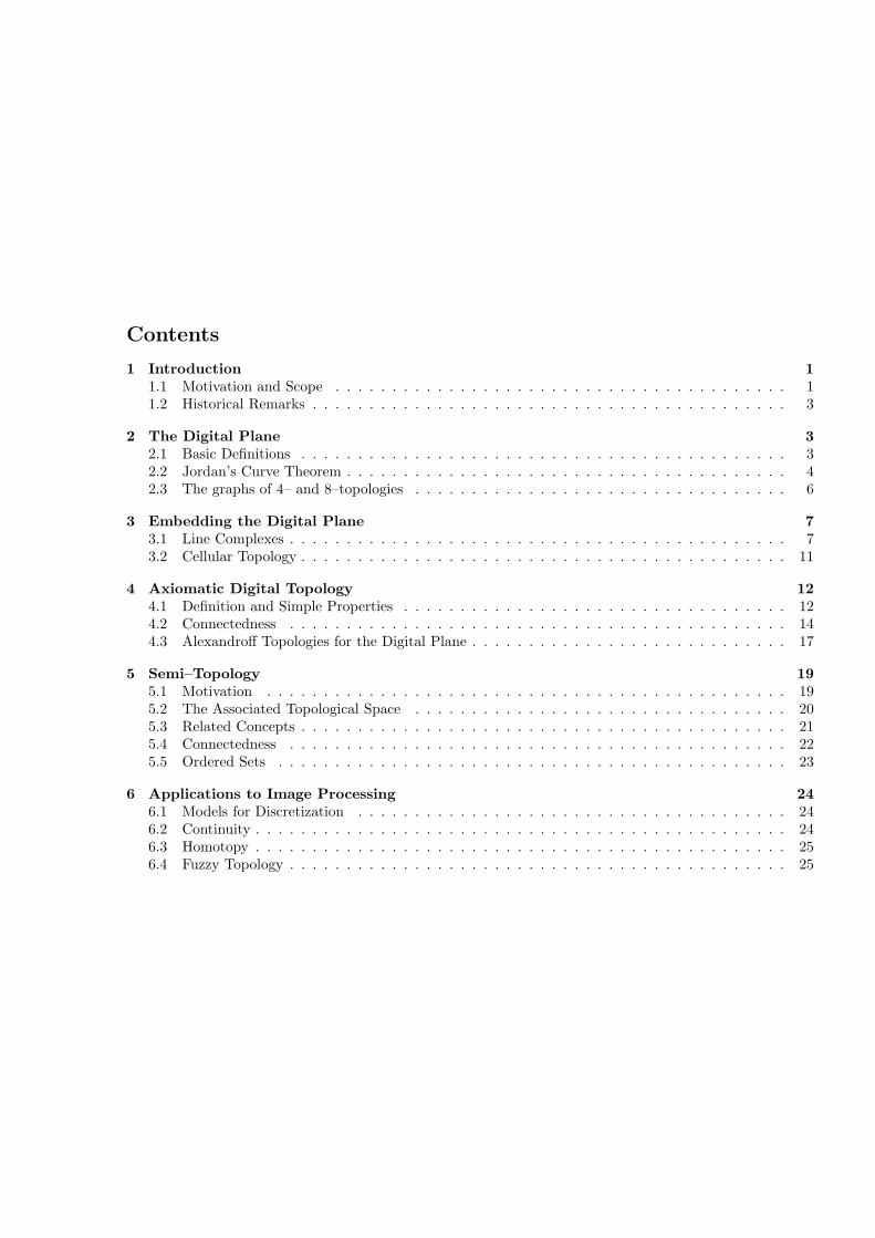
The sets OP and CP are given in the Table in Figure4. In the last column of this table the sets of vertexpoints associated to each point are given. The set ofall vertex points is Σ := {α, β, γ, δ}. X can be inter-preted as a square (see Figure 4). The vertex pointsof X are the vertices of the square, a, b, c and dcorrespond to the edges (without end points) and Qis the interior of the square.
This topological space is not complete since thereare no points in it belonging to tree–element vertex
13

sets. Also the sets {α, γ} and {β, δ} do not belong topoints in X . We can add in an obvious way elementsbelonging to these sets of vertex points. There are twonew edges e and f and four triangles F1, F2, F3, F4 asindicated in Figure 5. The completed topological spaceX can be visualized as a simplex in 3–space by rais-ing one vertex of the original square above the planedefined by the others. This is illustrated in Figure 6.
Locally finite Alexandroff spaces which are not T1
suffer from a very serious defect which severely lim-its their usage in image processing. We define in tueusual way: A function f mapping an topological spaceX into another topological space Y is termed contin-uous if for all sets U ⊆ Y which are open in Y theinverse image
f−1(U) := {x ∈ X | f(x) ∈ U}
is open in X.The following Theorem states that the set of all
continuous functions mapping a nontrivial locally fi-nite Alexandroff space into itself is subject to severerestrictions [40].
Theorem 9 Let X be a locally finite Alexandroffspace which is not T1.
Then there exist two points P 6= Q in X such thatfor every two neighborhoods U(P ) and U(Q) of thesepoints any injection f : U(P ) −→ U(Q) mapping Pin Q is not continuous.
Proof X is not T1, hence there exist points P andQ such that Q ∈ OP and P /∈ OQ. Thus OQ ⊂ OP(strictly), and therefore |OQ| < |OP |.
OP is clearly an open subset of U(P ) and OQ is anopen subset of U(Q). Let f : U(P ) −→ U(Q) be anycontinuous injection. Since P ∈ f−1(OQ) we obtainthat OP ⊆ f−1(OQ). Thus |OP | ≤ |f−1(OQ)| =|OQ|, and this contradicts the fact that |OQ| < |OP |.
2
A topological space is termed homogeneous, whenany two points of it have homeomorphic neighbor-hoods which means that there exist a bijective func-tion which maps one neighborhood onto the otherand together with its is inverse is continuous. Thenthe assertion of the Theorem can be formulated as
follows: Any Alexandroff space with nontrivial topol-ogy is not homogeneous.
The assertion of the Theorem is of course notcompletely surprising. For example, a function whichmaps vertices into edges in Example 1 should not becontinuous.
4.2 Connectedness
Let S be a subset of X. In the relative topology in-duced in S by the topology in X the open sets areall sets U ∩S with U open in X. One easily sees thatthis is indeed a topology in S. A set which is open inthe relative topology of S is a relatively open set.
The set S ⊆ X is termed connected if there is nodecomposition S = T1 ∪ T2 such that T1 ∩ T2 = ∅,both T1, T2 6= ∅ and relatively open with respect to S.Obviously, with respect to the indiscrete topology allsets are connected and for the strictly discrete topol-ogy only sets consisting of one point are connected.Therefore these topologies are not very interesting forinvestigating connectedness.
We now state a fundamental Lemma which re-lates the notion of connectedness defined here tothe more constructive and intuitive notion of path–connectedness.
Lemma 2 Let X = {P0, P1, · · · , Pn} be a finite set.There exist exactly two Alexandroff topologies on
X with the property that exactly all segments of con-secutive points Pi, Pi+1, · · · , Pj with 0 ≤ i < j ≤ nare connected sets.
These topologies are
T1 : OPi = {Pi} if i even,OPi = {Pi−1, Pi, Pi+1} if i 6= 1, n odd,OP1 = {P1, P2},OPn = {Pn−1, Pn}, if n odd.
and
T2 : OPi = {Pi} if i odd,OPi = {Pi−1, Pi, Pi+1} if i even and
i 6= n, n even,OPn = {Pn−1, Pn}, if n even.
14
P OP CP S
α {α, d, a, Q} {α} {α}
β {β, a, b,Q} {β} {β}
γ {γ, b, c,Q} {γ} {γ}
δ {δ, c, d,Q} {δ} {δ}
a {a,Q} {a, α, β} {α, β}
b {b, Q} {b, β, γ} {β, γ}
c {c,Q} {c, γ, δ} {γ, δ}
d {d, Q} {d, δ, α} {δ, α}
Q {Q} X {α, β, γ, δ}
c c
c cQ
α β
γδ
a
b
c
d
Figure 4: The topological space X corresponding to a square.
Proof The proof consists of three steps:1. First we prove that OPi does not contain any
point Pk with k 6= i− 1, i, i + 1.The set {Pi, Pk} ist not connected by definition
since i and k are not consecutive integers. Hence thereexists a neighborhood of Pi not containing Pk andvice versa. This implies Pk /∈ OPi.
2. |OPi| = 2 implies i = 1 or i = n.Assume OPi = {Pi, Pi+1} (i 6= n). If Pi /∈ OPi−1,
then {Pi−1, Pi} is not connected, contrary to assump-tion. Consequently Pi ∈ OPi−1.
From part 1. we get Pi+1 /∈ OPi−1. This impliesOPi−1 ∩ OPi = {Pi}, hence OPi = {Pi} containsonly one point, a contradiction.
The other possible cases are treated analogously.3. There remain the following possibilities
OPi = {Pi} orOPi = {Pi−1, Pi, Pi+1}
When |OPi| = 1 and |OPi+1| = 1 then theset {Pi, Pi+1} is not connected. When OPi ={Pi−1, Pi, Pi+1} and OPi+1 = {Pi, Pi+1, Pi+2} for
any i with 0 < i < n then OPi ∩OPi+1 = {Pi, Pi+1}is open which contradicts part 2.
As a result, one–point neighborhoods and three–point neighborhoods alternate along X which leavesonly the both possibilities of the Lemma. 2
As an immediate consequence we state
Corollary 1 If P0 = Pn then there exists an Alexan-droff topology for X such that exactly all segmentsof consecutive points on the cyclic sequence of points(numbered modulo n) are connected if and only if nis odd.
Example 2 Let X be the set Z of all integers. Weconsider the topologies generated by means of inter-sections and unions from the systems of open sets asdefined below:
1. Open sets are all semi–infinite intervals {n ∈Z | n ≥ n0}. The topology generated by this systemis an Alexandroff topology which is not locally finite.
2. The Marcus–Wyse topology is generated by the
15

c c
c c
��
��
��
���@@
@@
@@
@@
@@
α β
γδ
a
b
c
d
New vertices of the completed space:
e has vertex points β and δ,f has vertex points α and γ.
Faces of completed space:
F1 has vertex points α, β, γ,F2 has vertex points α, γ, δ,F3 has vertex points β, γ, δ,F4 has vertex points α, β, δ.
Figure 5: Completion of X .
s
s
s
c s
���������
(((((((((((
@@
@@
@@
@,,
,,
,,
,,
,,,����
α β
δ
γ
db
a
c
ef
Figure 6: The completed space X .
smallest open subsets of points n ∈ Z
O{n} ={
{n}, if n is even,{n− 1, n, n + 1}, otherwise.
The Marcus–Wyse topology is a locally finite Alexan-droff topology [45]. As a consequence of Lemma 2 wecan state that the Marcus–Wyse topology is the onlylocally finite Alexandroff topology for Z having theproperty that exactly the subsets consisting of consec-utive numbers are connected.
We note that the Marcus–Wyse topology of the in-tegers is not translation invariant. The translationT : Z −→ Z defined by T (i) = i + 1 maps even num-bers into odd numbers. Consequently, this translationis not continuous (see Theorem 9).
For the digital plane one can easily prove the fol-lowing Theorem.
Theorem 10 The 2–dimensional Marcus–Wysetopology given by the smallest open set of a pointP = (m,n)>
OP ={N4(P ) ∪ {P} if m + n is even,{P} otherwise.
is (up to a translation) the only locally finite Alexan-droff topology for Z2 with the property that a subsetof Z2 is connected with respect to this topology if andonly if it is 4–connected.
An analogous assertion holds for Rd.From the Corollary we get immediately the asser-
tion that it is not possible to find a topology for Z2
which induces 8–connectivity. In Figure 7 a closedpath with an odd number of vertices is shown whichproves the assertion [15, 39, 49].
For an Alexandroff space we define: A path withend points P and Q is a set {P = P0, P1, · · · , Pn =
16

cc
cc
��
��@@
@@
��
@@
@@
��
cc
cc
��
��@@
@@
��
@@
@@
��
cc
cc
��
��@@
@@
��
@@
@@
��
cc
cc
��
��@@
@@
��
@@
@@
��
cc
cc
��
��@@
@@
��
@@
@@
��cc
cc
��
��@@
@@
��
@@
@@
��
cc
cc
��
��@@
@@
��
@@
@@
��
cc
cc
��
��@@
@@
��
@@
@@
��
cc
cc
��
��@@
@@
��
@@
@@
��
cc
cc
��
��@@
@@
��
@@
@@
��cc
cc
��
��@@
@@
��
@@
@@
��
cc
cc
��
��@@
@@
��
@@
@@
��
cc
cc
��
��@@
@@
��
@@
@@
��
cc
cc
��
��@@
@@
��
@@
@@
��
cc
cc
��
��@@
@@
��
@@
@@
��cc
cc
��
��@@
@@
��
@@
@@
��
cc
cc
��
��@@
@@
��
@@
@@
��
cc
cc
��
��@@
@@
��
@@
@@
��
cc
cc
��
��@@
@@
��
@@
@@
��
cc
cc
��
��@@
@@
��
@@
@@
��cc
cc
��
��@@
@@
��
@@
@@
��
cc
cc
��
��@@
@@
��
@@
@@
��
cc
cc
��
��@@
@@
��
@@
@@
��
cc
cc
��
��@@
@@
��
@@
@@
��
cc
cc
��
��@@
@@
��
@@
@@
��
s ss
ss
ss
��
��@
@@@
@@
@@��
��
@@
@@
Figure 7: A closed path having an odd number of vertices can be found in the graph corresponding to8–topology.
Q} with the property Pi ∈ OPi+1 or Pi+1 ∈ OPi
for all i = 0, 1, · · · , n − 1. Obviously, by Lemma 2,a path is a connected set. This is easily seen by in-specting both possible topologies on a path. If a pathwere not connected, it would contain two consecutivepoints which belong to different (relative) neighbor-hoods on the path. This, however is not possible ineither topology of the Lemma.
A subset S of an Alexandroff space is termed path–connected if for any two points P,Q ∈ S there existsa path with end points P and Q which is completelycontained in S.
Theorem 11 A subset S of an Alexandroff space isconnected if and only if it is path–connected.
Proof 1. Assume that S is not connected. LetT1, T2 be the two relatively open sets in S accordingto the definition of connectedness. For a path froma point P in T1 to a point Q ∈ T2 there exists anumber i such that Pi ∈ T1 and Pi+1 ∈ T2. However,if Pi ∈ OPi+1 then Pi+1 ∈ T1 since T1 was assumedto be open which means that OP ⊆ T1 for all P ∈ T1.The same argument holds for Pi+1 ∈ OPi.
2. If S is connected, we define for P in S the set
SP = {Q ∈ S | there is a path from P to Q in S}.
SP is an open set since it is the union of all smallestneighborhoods of points which are path–connectedto P . Let Q ∈ S \ SP . Then OQ ∩ S is a relativelyopen set containing Q and OQ ∩ SP = ∅, otherwiseQ ∈ SP . This implies S \ SP is open, contradictingthe connectedness of S. 2
4.3 Alexandroff Topologies for theDigital Plane
It now is easily possible to define an Alexandrofftopology for the digital plane. We assign a vertexto each point in the digital plane. If we interpreteach smallest square of points in Z2 as the topologicalspace X as in Example 1, we get the 4–topology inthe sense that the vertices of X correspond to pointsin Z2 and edges symbolize connectedness of points.
In a similar way we can introduce an Alexandrofftopology which is related to 8–topology into the dig-ital plane. For this reason we interpret each smallest
17

s s ss
ssss s
PPPPPP������
PPPPPP�
��
����
���
LL
LLL
����
JJJ
AAAA
AAAA
����
����
��
QQQ
����
s s ss
ssss s
PPPPPP������
PPPPPP�
��
����
���
LL
LLL
����
JJJ
AAAA
AAAA
����
����
��
QQQ
����
s s ss
ssss s
PPPPPP������
PPPPPP�
��
����
���
LL
LLL
����
JJJ
AAAA
AAAA
����
����
��
QQQ
����
s s ss
ssss s
PPPPPP������
PPPPPP�
��
����
���
LL
LLL
����
JJJ
AAAA
AAAA
����
����
��
QQQ
����
s s ss
ssss s
PPPPPP������
PPPPPP�
��
����
���
LL
LLL
����
JJJ
AAAA
AAAA
����
����
��
QQQ
����
s s ss
ssss s
PPPPPP������
PPPPPP�
��
����
���
LL
LLL
����
JJJ
AAAA
AAAA
����
����
��
QQQ
����
s s ss
ssss s
PPPPPP������
PPPPPP�
��
����
���
LL
LLL
����
JJJ
AAAA
AAAA
����
����
��
QQQ
����
s s ss
ssss s
PPPPPP������
PPPPPP�
��
����
���
LL
LLL
����
JJJ
AAAA
AAAA
����
����
��
QQQ
����
s s ss
ssss s
PPPPPP������
PPPPPP�
��
����
���
LL
LLL
����
JJJ
AAAA
AAAA
����
����
��
QQQ
����
s s ss
ssss s
PPPPPP������
PPPPPP�
��
����
���
LL
LLL
����
JJJ
AAAA
AAAA
����
����
��
QQQ
����
s s ss
ssss s
PPPPPP������
PPPPPP�
��
����
���
LL
LLL
����
JJJ
AAAA
AAAA
����
����
��
QQQ
����
s s ss
ssss s
PPPPPP������
PPPPPP�
��
����
���
LL
LLL
����
JJJ
AAAA
AAAA
����
����
��
QQQ
����
s s ss
ssss s
PPPPPP������
PPPPPP�
��
����
���
LL
LLL
����
JJJ
AAAA
AAAA
����
����
��
QQQ
����
s s ss
ssss s
PPPPPP������
PPPPPP�
��
����
���
LL
LLL
����
JJJ
AAAA
AAAA
����
����
��
QQQ
����
s s ss
ssss s
PPPPPP������
PPPPPP�
��
����
���
LL
LLL
����
JJJ
AAAA
AAAA
����
����
��
QQQ
����
s s ss
ssss s
PPPPPP������
PPPPPP�
��
����
���
LL
LLL
����
JJJ
AAAA
AAAA
����
����
��
QQQ
����
Figure 8: Modeling 8–topology by the completed space X . Certain points are raised above the plane to geta model without extra vertices.
square as the completed space of Example 1. We canput together the simplices of the completed space ina three–dimenisonal model as shown in Figure 8.
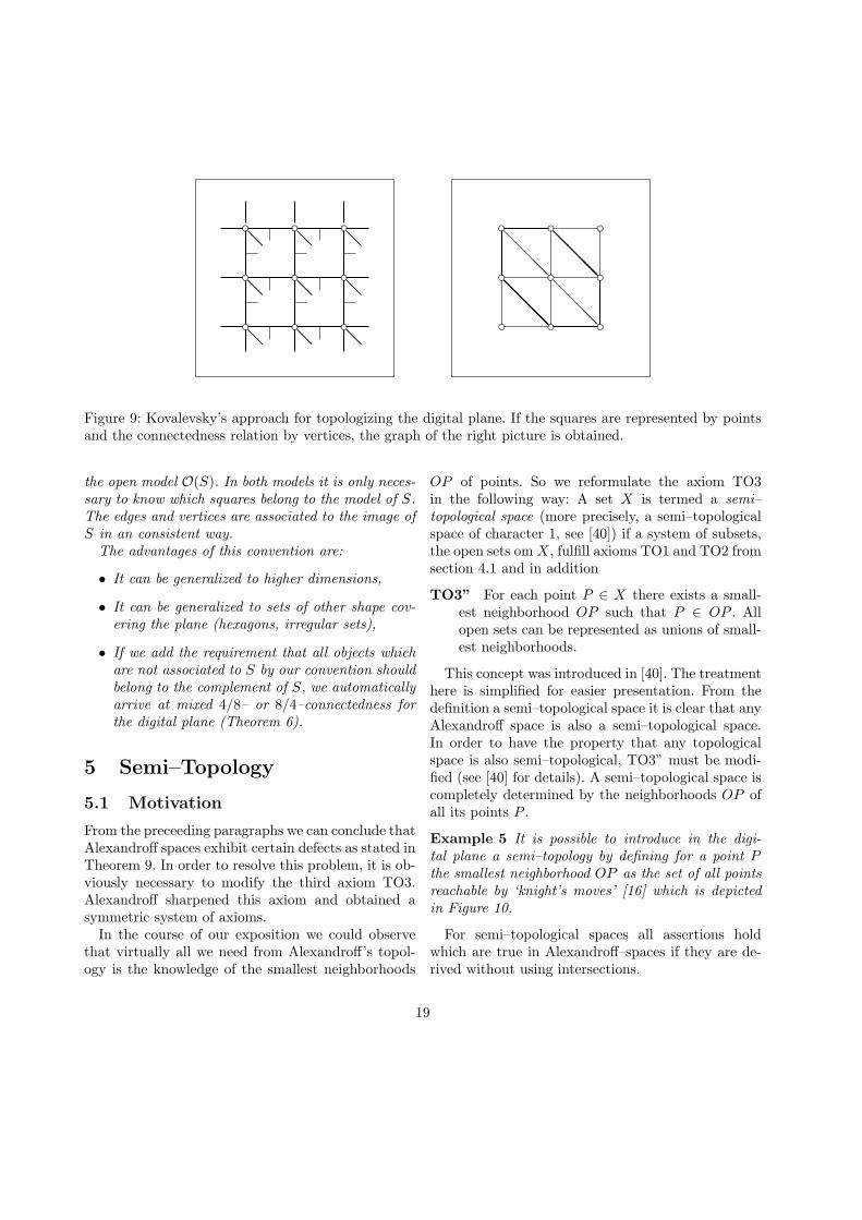
As an alternative we may associate to each pointin the digital plane a square as in the cellular model(see Figure 3). For each point in a digital set S (orequivalently, for each square) we must decide for fourvertices and four edges whether they should belongto S or not. This decision has to be done in such away that the subset of the plane thus obtained hasappropriate connectedness. In order to eliminate re-dundancy of these models, different authors proposedreduced models. We consider two examples.
Example 3 Kovalevsky [36] proposed that for anysquare belonging to a digital set S, the left and the up-per edge and the upper left vertex of the square should
belong to S. The connectedness structure induces intothe digital plane by this approach corresponds to the6–neighborhood which is equivalent to a covering ofthe plane by hexagons (see Figure 9). Therefore, inin the following picture, the two points • in the leftconfiguration are connected, in the right configurationthey are not connected.
c cs s s sc cExample 4 In the cellular model for digital topol-ogy (see Section 3.2) we investigated two continuousmodels for a digital set S, the closed model C(S) and
18
ccc
ccc
ccc
@@
@@
@@
@@
@@
@@
@@
@@
@@
ccc
ccc
ccc
@@
@@
@@
@@
@@
@@
@@
@@
@@
@@
@@
@@
Figure 9: Kovalevsky’s approach for topologizing the digital plane. If the squares are represented by pointsand the connectedness relation by vertices, the graph of the right picture is obtained.
the open model O(S). In both models it is only neces-sary to know which squares belong to the model of S.The edges and vertices are associated to the image ofS in an consistent way.
The advantages of this convention are:
• It can be generalized to higher dimensions,
• It can be generalized to sets of other shape cov-ering the plane (hexagons, irregular sets),
• If we add the requirement that all objects whichare not associated to S by our convention shouldbelong to the complement of S, we automaticallyarrive at mixed 4/8– or 8/4–connectedness forthe digital plane (Theorem 6).
5 Semi–Topology
5.1 Motivation
From the preceeding paragraphs we can conclude thatAlexandroff spaces exhibit certain defects as stated inTheorem 9. In order to resolve this problem, it is ob-viously necessary to modify the third axiom TO3.Alexandroff sharpened this axiom and obtained asymmetric system of axioms.
In the course of our exposition we could observethat virtually all we need from Alexandroff’s topol-ogy is the knowledge of the smallest neighborhoods
OP of points. So we reformulate the axiom TO3in the following way: A set X is termed a semi–topological space (more precisely, a semi–topologicalspace of character 1, see [40]) if a system of subsets,the open sets om X, fulfill axioms TO1 and TO2 fromsection 4.1 and in addition
TO3” For each point P ∈ X there exists a small-est neighborhood OP such that P ∈ OP . Allopen sets can be represented as unions of small-est neighborhoods.
This concept was introduced in [40]. The treatmenthere is simplified for easier presentation. From thedefinition a semi–topological space it is clear that anyAlexandroff space is also a semi–topological space.In order to have the property that any topologicalspace is also semi–topological, TO3” must be modi-fied (see [40] for details). A semi–topological space iscompletely determined by the neighborhoods OP ofall its points P .
Example 5 It is possible to introduce in the digi-tal plane a semi–topology by defining for a point Pthe smallest neighborhood OP as the set of all pointsreachable by ‘knight’s moves’ [16] which is depictedin Figure 10.
For semi–topological spaces all assertions holdwhich are true in Alexandroff–spaces if they are de-rived without using intersections.
19

ccccccc
ccccccc
ccccccc
ccccccc
ccccccc
ccccccc
cccccc
Ps s s ss s s s
Figure 10: Smallest neighborhood of point P in thesemi–topology induced by knight–moves in the digitalplane.
It is for example easy to define continuity in fullanalogy to continuity in topological spaces:
A function ϕ : X −→ Y mapping a semi–topological space X into a semi–topological space Yis continuous, if for each set S ⊆ Y which is openin Y the set ϕ−1(S) is open in X. ϕ is termed ahomeomorphism from X onto Y if the inverse func-tion ϕ−1 : Y −→ X exists and if ϕ and ϕ−1 are bothcontinuous functions. X and Y are termed homeo-morphic spaces in this case.
The following Theorem is trivial but of fundamen-tal importance since it illustrates a typical difficultyencontered in digital topology: Homeomorphic topo-logical spaces must have the same number of ele-ments.
Theorem 12 Let X be a semi–topological space con-sisting of finitely many elements.
Let Y be a semi–topological space and ϕ : X −→ Ya homeomorphism. Then Y has the same number ofelements as X.
For the proof of this Theorem we need only thebijectivity of ϕ.
In other words: The number of elements in a finiteset is a (semi–) topological invariant.
Analogously as for Alexandroff spaces a semi–topological space X is termed locally finite if OP hasa finite number of elements for all P ∈ X.
Let Y be a subset of a semi–topological space X.The relative semi–topology in Y which is induced bythe semi–topology in X is generated by the set of allneighborhoods OP ∩ Y .
Example 6 Consider again the set Z. We define theneighborhood O(n) = {n−1, n, n+1} for every n ∈ Z.This yields a semi–topology in Z which we will call thestandard semi–topology for Z.
5.2 The Associated Topological Space
There are some specialties with semi–topologicalspaces. Let S be an open subset of an Alexandroffspace. Then for each P ∈ S, the set OP is containedin S. This is not necessarily true in semi–topologicalspaces. Therefore we define: A subset S of a semi–topological space is strictly open if OP ⊆ S for allP ∈ S. Obviously, a strictly open set is also an openset.
Consider for example the Marcus–Wyse topologyin Z (see Example 2). In this topology each open setis strictly open.
Let X be a semi–topological space with topologyT . We introduce in X a second topology TA in whichthe strictly open sets are declared to be open. It iseasily seen that TA is indeed a topology for X.
By definition, each TA–open set is also T –openwhich is expressed in the language of general topol-ogy by saying that TA is coarser than T or T is finerthan TA. Specifically, for the smallest open neighbor-hoods of a point, OP with respect to T and OAPwith respect to TA, one always has OP ⊆ OAP .
Theorem 131. TA is either an Alexandroff topology or it is dis-
crete in the strict sense or it is indiscrete.2. Let T ′ be a topology fulfilling TO3’ which is
coarser than T . Then T ′ is coarser than TA.
Proof 1. Given a system {Sσ} of TA–open setsand P ∈ S :=
⋂Sσ. Then OP is contained in each
Sσ, hence in S. This proves TO3’ for TA.2. For P ∈ X let O′P be the smallest T ′–
neighborhood of P . Given a T ′–open set S, thenO′P ⊆ S for all P ∈ S, for otherwise O′P ∩ S would
20

be a neighborhood of P which is strictly contained inOP . This implies that S is TA–open. 2
We may restate part 2 of the Theorem in sayingthat TA is the finest topology with TO3’ which iscoarser than the semi–topology T . TA is termed thetopology associated to the semi–topology T . Accord-ing to the associated topology we may classify semi–topological spaces into three classes:
AT1 TA is discrete in the strict sense. Then thesame holds for T .
AT2 TA is an Alexandroff topology. Then T is alsoT0 but not T1 since
Q ∈ OP =⇒ Q ∈ OAP =⇒=⇒ P /∈ OAQ =⇒ P /∈ OQ.
AT3 TA is the indiscrete topology.
Spaces having property AT1 are not very interest-ing. Spaces with property AT2 are close relatives ofAlexandroff spaces. We note that in such spaces The-orem 9 holds. The proof of this Theorem literallycarries over to the semi–toplogical case when AT2is true. The most interesting spaces for our purposesare those having property AT3.
A semi–topological space is termed homogeneous iffor any two points P and Q the neighborhoods OPand OQ are homeomorphic. Homogeneity thereforecan be considered as ‘topological translation invari-ance’. The points of a homogeneous space cannot bedistinguished topologically. We saw that a nontrivialAlexandroff space is never homogeneous. Therefore,for a homogeneous semi–topological space the asso-ciated topology is either strictly discrete (AT1) orindiscrete (AT3).
A semi–topological space X is termed symmetricif Q ∈ OP implies P ∈ OQ for all P,Q ∈ X. FromTheorem 7 we know that an Alexandroff space is cer-tainly not symmetric. Therefore, a symmetric semi–topological space belongs either to class AT1 or toclass AT3.
Example 7 The space Z, if equipped with thestandard–semi–topology, is a symmetric semi–topo-logical space.
The Marcus–Wyse topology was introduced in a“semi–topological” way by means of smallest openneighborhoods (see Example 2):
O(n) ={
{n}, if n is even,{n− 1, n, n + 1}, else.
This topology, however, does not make Z a symmetricspace since for example 0 ∈ O(1) = {0, 1, 2} and 1 /∈O(0) = {0}. Clearly, the Marcus–Wyse topology isalso not homogeneous.
5.3 Related Concepts
There are some concepts in the literature whichcan be easily expressed in the framework of semi–topology. We consider some examples:
Example 8 Arnaud, Lamure, Terrenoire undTounissoux [8] proposed for image processing thepre–topological spaces of Brissaud [12].
For a set X let P(X) be the set of all subsets of X.a : P(X) −→ P(X) is termed the closure–mappingand has the properties
S ⊆ a(S) fur alle S ⊆ X
and a(∅) = ∅. The set X equipped with the mappinga is termed a pre–topological space.
For a semi–topological space X we define a(S) =⋃P∈S OP which makes X a pre–topological space.There do exist pre–topological spaces which are
not semi–topological spaces. Consider for example thespace Z with the pre–topology
a(S) ={{n− 1, n, n + 1}, if S = {n},
S else,
then Z is not a semi–topological space, since it is notpossible to represent all sets a(S) as union of smallestneighborhoods. Consider for example a set consistingof two consecutive points in Z.
Example 9 Given a symmetric homogeneous semi–topological space X. Then all OP are homeomorphicto a subset B0 in X.
21
For a set S ⊆ X we define the dilation of S withstructuring element B0 as
DIL(S) =⋃
P∈S
OP
and the erosion of S
ERO(S) = {P | OP ⊆ S} .
We note that DIL(S) corresponds to the seta(S) in Example 8 and ERO(S) corresponds toC
⋃P∈CS OP . One has
ERO(S) ⊆ S ⊆ DIL(S).
Both these sets associated to a given set are usedto analyze sets. For example, one might ask, underwhich circumstances DIL(ERO(S)) = S or how thepoints can be characterized where both these sets dif-fer. It is also possible to investigate the iterated setsDILk(S) and so on.
These questions belong to the field of mathematicalmorphology and are treated for example in Serra’sbooks [57, 58].
5.4 Connectedness
If we translate connectedness in semi–topologicalspaces verbally from Alexandroff spaces, we get a re-sult which is not desirable:
Example 10 In the standard semi–topology for Zthe sets {1, 2, 3} and {4, 5, 6} are open. If we applythe definition of connectedness in a naive way, theset {1, 2, 3, 4, 5, 6} would not be connected.
We therefore define: The set S ⊆ X is termed con-nected if there is no decomposition S = T1 ∪ T2 suchthat T1 ∩ T2 = ∅, both T1, T2 6= ∅ and both strictly(relatively) open with respect to S.
We note, that a set is T –connected whenever it isTA–connected. The converse is not necessarily true,since for example in AT3–spaces all subsets are TA–connected but not always T –connected.
Example 11 Let S be a subset of Z, equipped withthe standard semi–topology (see Example 6). Then
it is not possible to have a representation S =⋃{O(n) | n ∈ S}, hence there exists no strictly open
subset of Z (in the standard semi–topology). This im-plies that Z is trivially a connected space.
We know that exactly the subsets of consecutivenumbers are connected in Z with respect ot theMarcus–Wyse topology (see Example 2). This asser-tion is also true in the standard semi–topology.
Example 12 In a pre–topological space (see Exam-ple 8) the definition of connectedness is much morecomplex. A subset S of a pretopological space is con-nected if there exist two sets F and G such that
• F =⋃
Fj, G =⋃
Gj,
• S ⊆ F ∪G,
• S ∩⋃
a(Fj) 6= ∅,
• S ∩⋃
a(Gj) 6= ∅,
• S ∩⋃
a(Fj) ∩⋃
a(Gj) = ∅,
Obviously, in a semi–topological space both definitionsof connectedness coincide.
The advantage of semi–topological spaces over pre–topologcial spaces is that the definitions in semi–topology are very close to those in general topologyas we have seen for continuity and connectedness.Therefore it is possible to translate a large number ofassertions from general topology almost literally intosemi–topology.
Since nontrivial symmetric semi–topological spacesare always AT3–spaces, we can state that a symmet-ric semi–topological space is not connected if andonly if it contains a nonempty strict subset whichis strictly open.
Example 13 In the digital plane we introduce thesemi–topologies Tκ for κ ∈ {4, 8} by the smallest opensets Oκ(P ) = Nκ(P )∩{P}. Both these topologies arehomogeneous and symmetric. Tκ–connectedness is thesame as κ–connectedness defined in Section 2.
In a semi–topological space we can find a theoremwhich is analogous to Theorem 11. We first define a
22
path just as in case of Alexandroff spaces. By inspec-tion of the proof of Theorem 11 we see that it canbe easily adapted to semi–topological spaces by re-placing ‘open’ by ‘strictly open’. The Theorem nowreads
Theorem 14 A subset S of an semi–topologicalspace is connected if and only if it is path–connected.
In a semi–topological space Lemma 2 is not truesince there are more than two possibilities to (semi–)topologize a path. This generates more freedom forconstruction and this freedom is sufficient to allowfor any closed path a topology in contrast to Corol-lary 1. So it is easily possible to find a semi–topologywhich causes the digital plane to be 8–connected (seeExample 13).
There is even another advantage of semi–topology.We know that in ordinary topology curves in thedefinition of connectedness are introduced as home-omorphic images of a real interval. This means thatwe compare the topology of a given space with thewell–known topology of the reals (or integers, respec-tively). In symmetric semi–topological spaces we canuse the concept of continuity for introducing connect-edness.
A subset Y of a semi–topological space X is termedan arc if it is a homeomorphic image of an intervalin Z, where Z is equipped with the standard semi–topology. A subset S of a semi–topological space istermed arc–connected if for any two points in S thereexists an arc which is completely contained in S andwhich contains both points.
We now state
Lemma 3 A subset Y of a symmetric semi–topological space is an arc if and only if it is a simplepath (i.e. a path {P0, P1, · · · , Pn} such that exactlythe subsets of consecutive points are connected).
Proof 1. Assume that Y is an arc with homeo-morphism ϕ : [0, n] −→ W , where ϕ(i) = Pi. Thenthe smallest neighborhood of a point Pi ∈ W is thehomeomorphic image of the smallest neighborhoodof i ∈ Z in the standard semi–topology. Thus, OPi
contains exactly Pj ∈ Y with |i− j| ≤ 1.
2. Let Y = {P0, P1, · · · , Pn} be a simple path inX. ϕ(i) = Pi is bijective. Since X is symmetric, bydefinition of a path, OPi contains Pj ∈ Y with |i −j| ≤ 1. Since Y is simple, OPi does not contain anyother points in S. Hence, OPi is homeomorphic toO(i). 2
We can conclude that for symmetric semi–topological spaces connectedness, path–connected-ness and arc–connectedness are equivalent.
5.5 Ordered Sets
We add here a different approach to digital topol-ogy which dates back to Alexandroff. This approachuses the concept of partially ordered set (‘poset’) andplays a role in computer science (see e.g. [10]). Al-though there is a large amount of literature about thistopic, we only sketch it and relate it to the structuresdeveloped here.
A set X is called a partially ordered set if it isequipped with a relation v such that
PO1 P v P for all P ∈ X,
PO2 P v Q and Q v R implies P v R,
PO3 P v Q and Q v P implies P = Q.
A set x is called an ordered set if in addition
PO4 For all P ∈ X is P v Q or Q v R.
In an Alexandroff space X we introduce the partialorder relation
Q v P ⇐⇒ Q ∈ CP.
For the proof that this is indeed a partial order,we need Part 1 of Theorem 7. Since this assertionis not generally true in semi–topological spaces, weconclude that such an order relation does not alwaysexist in semi–topological spaces.
Conversely, if X is a partially ordered set with or-der relation v, we can define in analogy to semi–topology
CP = {Q | Q v P}.
23

We note that this definition is indeed ‘semi–topological’ since we define smallest closed sets con-taining a point and then generate the whole topologyby means of unions of such sets. In contrast to semi–topology, we do not start with open neighborhoodsbut it seems to be relatively clear that we arrive inthis way at some sort of (semi–) topology.
When we consider Example 1 then Q v P meansgeometrically that Q is a boundary element of P . In-deed, we can interpret Alexandroff spaces as abstractcell complexes. This was demonstrated in [1].
As Alexandroff spaces and partially ordered spacesare equivalent, we can start our theory as well withthe latter. This is usually done for modeling discretestructures in computer science [56].
Khalimsky [21, 26, 27] investigated connected or-dered topological spaces (COTS). Such spaces X arecharacterized by the properties that they are con-nected and that among each triple of points P , Q,R there is one, say Q, which has the property thatX \ {Q} consists of exactly two connected compo-nents, each containing one of the both remainingpoints. These spaces can be considered as homeomor-phic images of intervals in R or Z, hence they are ide-ally suited for defining paths and path–connectednessin discrete structures.
6 Applications to Image Pro-cessing
We restrict ourselves here to some applications of dig-ital topology to image processing.
6.1 Models for Discretization
A very important and fundamental problem in imageprocessing can be stated as follows: Given a set S inthe Euclidean space R2 and let ∆ : R2 −→ Z2 be adiscretization mapping which associates to S a dis-crete set ∆(S). Such a mapping can be considered asa model of a digitizer. There were different such map-pings proposed in the literature, we mention Pavlidis’‘sampling theorem’ [50] and Serra’s book [58, Part II,Chapter VII]. More modern presentations of the sub-ject were given in [37] and [19].
Typical questions arising in this context are:
• Which topological (geometrical) properties doesthe discretized set ∆(S) share with the set S?
• Is ∆ or ∆−1 (as a point–to–set mapping) contin-uous?
• Which other properties has ∆?
The problem of finding a continuous model for agiven discrete space is in some sense the inverse prob-lem of discretization.
6.2 Continuity
There is a need for defining continuity in the con-text of digital spaces [51]. This concept has proved asa very strong and fruitful one in ordinary topology.We have seen in the definition of arc–connectednessin semi–topological spaces that by continuity it be-comes possible to deduce a property of a topologicalspace from known properties of another space. If weinterpret the smallest neighborhoods of a point asa formal definition of ‘nearness’ (P and Q are nearof each other if P ∈ OQ or Q ∈ OP ), then con-tinuous functions are functions preserving nearness.Moreover, also connectedness is preserved under con-tinuos mappings.
An important tool is homeomorphy which allows tosolve certain problems by posing them in appropriatehomeomorphic spaces. A very difficult question aris-ing in this context is the problem of the dimension ofa digital space. We saw that the 8–topology inducesa graph structure which is not planar. The questionis, whether one can tell from the structure of a graphwhether it is a model for a plane (or more generally,a d–dimensional space) or not. This problem was in-vestigated in [49].
Typical questions in the context of continuity are:
• The intermediate value theorem of classical anal-ysis is a very powerful tool for solving nonlinearequations. Rosenfeld [51] was able to find a dig-ital analog of this theorem.
• A very important constructive tool in generaltopology is the fixed point principle which char-acterizes conditions under which a continuous
24
function f mapping a topological space into it-self has a fixed point x with f(x) = x. Rosenfeld[51] formulated a ‘near fixed point theorem’.
• Are different models of discrete spaces homeo-morphic?
6.3 Homotopy
Topological predicates are in a certain sense diffi-cult to handle on parallel computers as mentionedin Section 3. On the other hand, the large amountof data, which is typical for image processing appli-cations, calls for parallel processing. Therefore it wasproposed very early to reduce images to a ‘simple’topological equivalent before closer investigation oftopological predicates. Indeed, Rosenfeld showed in1979 [53] that the decision whether a simgle point ofa digital set influences its connectedness or the con-nectedness of its complement, can be made locallysince it can be shown to be a predicate only depend-ing on Euler’s number.
In Figure 11 the reduction process is illustrated.This procedure is known in the image processing lit-erature as ‘thinning’ or ‘skeletonization’. The reducedset or skeleton shown in the Figure was obtained byapplying a method described in [18] which is charac-terized by the property of being invariant with re-spect to motions of the digital plane. In order todescribe the thinning procedure in terms of homo-topy theory, it would be desirable to interpret thereduced image as a ‘deformation retract’ of the orig-inal one. However, there is no such possibility withinthe framework of digital topology or semi–topologyto deform the original image in a continuous way intothe reduced image. By Theorem 12 there is no wayto find a homeomorphism between finite sets havingdifferent numbers of elements.
Kong [28, 32] introduced a concept of digital homo-topy theory. This approach is based on an embeddingprocedure which is similar to the cellular model pre-sented in Section 3.2. The cellular images of the orig-inal image and the reduced image are indeed homeo-morphic in the R2 topology.
6.4 Fuzzy Topology
Digital topology is the theoretical basis for under-standing certain properties of sets in images, i.e. itis mainly suited to black–white images or to ‘seg-mented’ objects in images. An interesting problem isthe question, whether it is possible to generalize theknown concepts from black–white topology to gray–value topology. This is indeed possible by using con-cepts from ‘fuzzy topology’. Gray–value images pro-vide in some sense a very neat application of fuzzyset theory, since they exhibit a naturally given mem-bership function, the gray–value function. Rosenfeld[54] presented a theory of fuzzy topology for gray–value images. He was able to generalize such con-cepts as connectedness, area and circumference andcompactness of an object in an image. Since then, alarge number of papers dealing with this subject werepublished.
References
[1] P. Alexandroff. Diskrete Raume. MatematiceskiıSbornik (Receul Mathematique), 2 (44), N.3:502–519, 1937.
[2] Paul Alexandroff und Heinz Hopf. Topolo-gie, Erster Band: Grundbegriffe der mengen-theoretischen Topologie · Topologie der Kom-plexe · Topologische Invarianzsatze und an-schließende Begriffsbildungen · Verschlingungenim m–dimensionalen euklidischen Raum · stetigeAbbildungen von Polyedern, (Die Grundlehrender mathematischen Wissenschaften in Einzel-darstellungen, Band XLV), Verlag von JuliusSpringer, Berlin, 1935.
[3] A. D. Alexandrow. Konvexe Polyeder , (Math-ematische Lehrbucher und Monographien, II.Abteilung, Band VIII), Berlin: Akademie–Verlag, 1958.
[4] J. P. Auray and G. Duru. Fuzzy pretopologicalstructures and formation of coalitions. Theoryand application of digital control, Proc. IFACSymp., New Delhi 1982 , 459–463 (1982).
25

Figure 11: Reduction of an image. Points are deleted which do not affect the topology of the image. Deletedpoints are marked ‘’, remaining points are marked ‘ ’.
[5] J. P. Auray, G. Duru et M. Mougeot. Une meth-ode de comparaison des structures productivesdes pays de la C.E.E. Publ. Econ., 13(2):31–59,1980.
[6] Jean–Paul Auray, Gerard Duru and MichelMougeot. Some pretopological properties ofinput–output models and graph theory. Oper.Res. Verfahren, 34:5–21, 1979.
[7] J. P. Auray, M. Brissaud et G. Duru. Connexitedes espaces preferencies. Cah. Cent. Etud. Rech.Oper., 20:315–324, 1978.
[8] G. M. Arnaud, M. Lamure, M. Terrenoire andD. Tounissoux. Analysis of the connectivity
of an object in a binary image: pretopologi-cal approach. In: Eighth International Con-ference on Pattern Recognition, Paris, France,October 27–31,1986, Proceedings, pages 1204–1206. IEEE Computer Society Press, Washing-ton, D.C., 1986.
[9] K. H. Baik and L. L. Miller. Topological ap-proach for testing equivalence in heterogeneousrelational databases. The Computer Journal ,33:2–10, 1990.
[10] H. P. Barendregt. The Lambda Calculus — ItsSyntax and Semantics, Revised Edition, ElsevierScience Publishers B.V., North–Holland, Ams-terdam, New York, Oxford, 1984.
26

[11] Wilhelm Blaschke. Vorlesungen uber Integralge-ometrie, Dritte Auflage. Deutscher Verlag derWissenschaften, Berlin, 1955.
[12] Marcel Brissaud. Les espaces pretopologiques.Comptes Rendus hebdomadaires des Seances del’Academie des Sciences, 280, Serie A:705–708,1975.
[13] Marcel Brissaud. Structures topologiques desespaces preferencies. Comptes Rendus hebdo-madaires des Seances de l’Academie des Sci-ences, 280, Serie A:961–964, 1975.
[14] Marcel Brissaud. Agregation des preferences in-dividuelles. Comptes Rendus hebdomadaires desSeances de l’Academie des Sciences, 278, SerieA:637–639, 1974.
[15] Jean–Marc Chassery. Connectivity and consec-utivity in digital pictures. Computer Graphicsand Image Processing , 9:294–300, 1979.
[16] P. P. Das and B. N. Chatterji. Knight’s distancein digital geometry. Pattern Recognition Letters,7:215–226, 1988.
[17] R. O. Duda, P. E. Hart and J. H. Munson.Graphical Data Processing Research Study andExperimental Investigation. AD650926, March1967, pages 28–30.
[18] Ulrich Eckhardt and Gerd Maderlechner. Invari-ant thinning. International Journal of PatternRecognition and Artificial Intelligence), (SpecialIssue on Techniques for Thinning Digitized Pat-terns), 7:1115–1144, 1993.
[19] Ari Gross and Longin Latecki. Digitizationsperserving topological and differential geomet-ric properties. CVGIP: Image Understanding ,(to appear).
[20] P. M. Gruber and C. G. Lekkerkerker. Geome-try of Numbers, Second Edition, North–HollandMathematical Library, Volume 37 , (First edi-tion as Bibliotheca Mathematica, Volume VIII ,1969). Amsterdam: North–Holland PublishingCompany, New York: Elsevier Publishing Co.,Inc. 1987.
[21] Efim Davidovic Halimskiı. Ordered TopologicalSpaces, (Russian), Academy of Sciences of theUkrainian SSR, Naukova Dumka, Kiev, 1977.
[22] Frank Harary. Graph Theory , Addison–WesleyPublishing Company, Reading, Massachusetts,Menlo Park, California, London, Don Mills, On-tario, 1969.
[23] Gabor T. Herman. Discrete multidimensionalJordan surfaces. CVGIP: Graphical Models andImage Processing , 54:507–515, 1992.
[24] Gabor T. Herman. On topology as applied toimage analysis. Computer Vision, Graphics, andImage Processing , 52:409–415, 1990.
[25] John L. Kelley. General Topology , (The Uni-versity Series in Higher Mathematics), D. VanNostrand Company, Inc., Princeton, New Jersey,Toronto, London, New York, 1955.
[26] Efim Khalimsky, Ralph Kopperman and Paul R.Meyer. Computer graphics and connectedtopologies on finite ordered sets. Topology andits Applications, 36:1–17, 1990.
[27] E. Khalimsky. Topological structures in com-puter science. Journal of Applied Mathematicsand Simulation, 1:25–40, 1987.
[28] T. Y. Kong, A. W. Roscoe and A. Rosenfeld.Concepts of digital topology. Topology Appl.,46:219–262, 1992.
[29] T. Y. Kong and E. Khalimsky. Polyhedralanalogs of locally finite topological spaces. In:R. M. Shortt, ed.: General Topology and Ap-plications, Lecture Notes in Pure and AppliedMathematics, Volume 123 , pages 153–163. NewYork, Basel: Marcel Dekker, Inc. 1990.
[30] T. Y. Kong and A. Rosenfeld. If we use 4– or8–connectedness for both the objects and thebackground, the Euler characteristic is not lo-cally computable. Pattern Recognition Letters,11:231–232, 1990.
27
[31] T. Y. Kong and A. Rosenfeld. Digital topol-ogy: Introduction and survey. Computer Vi-sion, Graphics, and Image Processing , 48:357–393, 1989.
[32] T. Y. Kong. A digital fundamental group. Com-puters & Graphics, 13:159–166, 1989.
[33] T. Y. Kong and A. W. Roscoe. Continuousanalogs of axiomatized digital surfaces. Com-puter Vision, Graphics, and Image Processing ,29:60–86, 1985.
[34] Ralph Kopperman, Paul R. Meyer andRichard G. Wilson. A Jordan surface the-orem for three–dimensional digital spaces.Discrete Comput. Geom., 6:155–161, 1991.
[35] Ralph Kopperman and Yung Kong. Using gen-eral topology in image processing. In: U. Eck-hardt, A. Hubler, W. Nagel and G. Werner, ed-itors: Geometrical Problems of Image Process-ing. Proceedings of the 5th Workshop held inGeorgenthal, March 11–15, 1991. (Research inInformatics, Volume 4), pages 66–71. Berlin:Akademie–Verlag 1991.
[36] V. A. Kovalevsky. Finite topology as applied toimage analysis. Computer Vision, Graphics, andImage Processing , 45:141–161, 1989.
[37] E. H. Kronheimer. The topology of digital im-ages. Topology and its Applications, 46:279–303,1992.
[38] Longin Latecki, Ulrich Eckhardt and AzrielRosenfeld. Well–Composed Sets. CVGIP: ImageUnderstanding , (to appear).
[39] Longin Latecki. Topological connectedness and8–connectedness in digital pictures. CVGIP: Im-age Understanding , 57:261–262, 1993.
[40] Longin Latecki. Digitale und Allgemeine Topolo-gie in der bildhaften Wissensreprasentation.(DISKI Dissertationen zur Kunstlichen Intelli-genz 9), infix, St. Augustin, 1992.
[41] Chung–Nim Lee, Timothy Poston and AzrielRosenfeld. Holes and genus of 2D and 3D digi-tal images. CVGIP: Graphical Models and ImageProcessing , 55:20–47, 1993.
[42] Chung–Nim Lee, Timothy Poston and AzrielRosenfeld. Winding and Euler numbers for 2Dand 3D digital images. CVGIP: Graphical Mod-els and Image Processing , 53:522–537, 1991.
[43] Norman Levitt. The Euler characteristic is theunique locally determined numerical homotopyinvariant of finite complexes. Discrete Comput.Geom., 7:59–67, 1992.
[44] E. A. Lord and C. B. Wilson. The mathematicaldescription of shape and form,Chichester: Ellis Horwood Limited; New York,Chichester, Brisbane, Toronto: John Wiley &Sons 1986.
[45] Dan Marcus, Frank Wyse et al. A special topol-ogy for the integers (Problem 5712). Amer.Math. Monthly , 77:1119, 1970.
[46] G. Matheron. Random Sets and Integral Geom-etry , John Wiley & Sons, New York, London,Sydney, Toronto, 1975.
[47] Hermann Minkowski. Geometrie der Zahlen,B. G. Teubner, Leipzig und Berlin, 1910. (John-son Reprint Corporation, New York, London,1968).
[48] Marvin Minsky and Seymour Papert. Percep-trons. An Introduction to Computational Ge-ometry , The MIT Press, Cambridge, Mas-sachusetts, London, England, 1969.
[49] Daniel Nogly und Markus Schladt. Grund-lagen einer diskreten Geometrie auf Graphenals Tragerstrukturen, Diplomarbeit UniversitatHamburg, Institut fur Angewandte Mathematik ,April 1992.
[50] Theodosios Pavlidis. Algorithms for Graphicsand Image Processing , Springer–Verlag (Com-puter Science Press), Berlin, Heidelberg, 1982.
28

[51] Azriel Rosenfeld. ‘Continuous’ functions on digi-tal pictures. Pattern Recognition Letters, 4:177–184, 1986.
[52] Azriel Rosenfeld. Three–dimensional digitaltopology. Inform. and Control , 50:119–127,1981.
[53] Azriel Rosenfeld. Digital topology. AmericanMathematical Monthly , 86:621–630, 1979.
[54] Azriel Rosenfeld. Fuzzy digital topology. Infor-mation and Control , 40:76–87, 1979.
[55] Dana Scott. Data types as lattices. SIAM J.Comput., 5:522–587, 1976.
[56] Dana Scott. Outline of a mathematical theory ofcomputation. In Proceedings of the Fourth An-nual Princeton Conference on Information Sci-ences and Systems (1970), pages 169–176.
[57] Jean Serra, editor. Image Analysis and Mathe-matical Morphology, Volume 2: Theoretical Ad-vances, Academic Press, Harcourt Brace Jo-vanovich Publishers, London, San Diego, NewYork, Boston, Sydney, Tokyo, Toronto, 1988.
[58] Jean Serra. Image Analysis and MathematicalMorphology , Academic Press, Inc., London, Or-lando, San Diego, New York, Austin, Boston,Sydney, Tokyo, Toronto, 1982.
[59] D. Stoyan, W. S. Kendall and J. Mecke. Stochas-tic Geometry and Its Applications, John Wi-ley & Sons, Chichester, New York, Brisbane,Toronto, Singapore, 1987.
29