Embed Size (px)
Citation preview
DIGITAL SIGNAL PROCESSING — FALL 2015
This course provides a comprehensive introduction to the use of Fourier methods in digital signal processing.
COURSE INFORMATION
Instructor: Jim Walker
Office: 527 Hibbard
E-mail: walkerjs
Office Hours
Mondays, Thursdays, and Fridays: 11:00 am to Noon, 2:00 to 2:30 pm. Or, by appointment.
Text
The texts for the course are Fourier Analysis by J.S. Walker and A Primer on Wavelets and their Scientific
Applications, 2nd Edition by J.S. Walker.
Software
Software for the course is the freeware FAWAV which can be downloaded from the web site:
http://www.uwec.edu/walkerjs/FAWAVE/
It is also available on the Virtual Lab, under Departmental/Mathematics. The Virtual Lab implementation is
probably the best for non-Windows operating systems, such as Macs.
Grading
Your grade for the course will be determined by your performance on the graded homework, and three exams.
The following percentages will be used:
Selected Homework 25%
3 Exams (25% each) 75%
Students with Disabilities
Any student who has a disability and is in need of classroom accommodations, please contact the instructor
and the Services for Students with Disabilities Office in Old Library 2136 at the beginning of the semester.
Note: You will need to supply me with one copy of your VISA form for the Math Dept Office’s records.
1
2 DIGITAL SIGNAL PROCESSING — FALL 2015
SYLLABUS
• Fourier Series
– Basic theory
– Convergence
– Applications to sound
∗ Harmonics (periodic signals corresponding to frequencies)
∗ Parseval’s equality
– Test 1
• Discrete Fourier Analysis
– DFTs
– FFTs
– Gabor transforms
– Applications
∗ musical instruments
∗ voice analysis
∗ musical analysis
∗ sound synthesis
∗ denoising
∗ multiple signal transmission (frequency multiplexing)
∗ scalograms
– Test 2
• Fourier Transforms
– Basic theory
– Inversion
– Applications to telecommunications
∗ Sampling theory
∗ multiple signal transmission (time multiplexing)
– Cosine transforms and spectroscopy
– Test 3
PART 1: FOURIER SERIES
1. INTRODUCTORY MATERIAL
What is Fourier analysis? Fourier analysis is the abstract science of frequency (periodic repetition). Fre-
quencies can occur over time or space, or even within the analysis of symmetries in more abstract geometries.
In this course we shall emphasize frequencies over time in sound signals.
Homework. Use FAWAV to graph the following functions.
1.1. x2 on the interval [−2, 2].
1.2. cos(3x)− 2 sin(4x) on the interval [−2π, 2π].
1.3. e−2x on the interval [0, 10].
1.4. e−2x cos 8πx+ e−2x sin 6πx on the interval [0, 15].
DIGITAL SIGNAL PROCESSING — FALL 2015 3
2. FOURIER SERIES DEFINED
Fourier series are used in analyzing the frequency content of periodic signals. Two basic examples are the
functions
cos rx and sin rx
where x typically stands for time in seconds, and r is a positive constant. They each have fundamental
(smallest) period of 2π/r. That is, they go through one cycle in 2π/r sec. Hence they have frequencies of
1/(2π/r) = r/(2π) cycles/sec (Hz).
Example. Find the fundamental period of cos 2x+ 3 sin 5x.
Solution. The first term cos 2x has periods of π, 2π, 3π, . . . . The second term 3 sin 5x has periods 2π/5, 4π5,
6π/5, . . . . The smallest common value among these two sets is 2π. Hence cos 2x+3 sin 5x has fundamental
period 2π.
Trigonometric system, period 2π. For analyzing signals of period 2π we use the following system of func-
tions:
1, cos x, sinx, cos 2x, sin 2x, . . . , cosnx, sinnx, . . .
which is called the trigonometric system, period 2π. Based on this system, the Fourier series for a function
f(x) of period 2π is
c0 +∞∑
n=1
(An cosnx+Bn sinnx)
where the Fourier coefficients are defined by
c0 =1
2π
∫ π
−πf(x) dx, An =
1
π
∫ π
−πf(x) cosnx dx, Bn =
1
π
∫ π
−πf(x) sinnx dx.
It is worth noting that, in order for a Fourier series to be defined, the function f(x) need only be defined over
the interval [−π, π] in such a way that the integrals for the Fourier coefficients are finite.
Examples. (1) Suppose f(x) = x on [−π, π) and has period 2π. Then its Fourier coefficients are computed
as follows:
c0 =1
2π
∫ π
−πx dx = 0 (x odd)
An =1
π
∫ π
−πx cosnx dx = 0 (x cosnx odd)
Bn =1
π
∫ π
−πx sinnx dx
=2
π
∫ π
0x sinnx dx (x sinnx even)
=2
π
[x− cosnx
n− (1)
− sin nx
n2
]∣∣∣∣π
0
(integrate by parts)
=2(−1)n+1
n.
Hence its Fourier series is∞∑
n=1
2(−1)n+1
nsinnx. (1)
4 DIGITAL SIGNAL PROCESSING — FALL 2015
(2) Suppose f(x) = |x| on [−π, π) and has period 2π. Then its Fourier coefficients are
c0 =1
2π
∫ π
−π|x| dx
=1
π
∫ π
0x dx =
π
2
An =1
π
∫ π
−π|x| cos nx dx
=2
π
∫ π
0x cosnx dx
=2
π
[xsinnx
n− (1)
− cos nx
n2
]∣∣∣∣π
0
=2
π
cosnπ − 1
n2
Bn =1
π
∫ π
−π|x| sinnx dx = 0.
Hence its Fourier series is
π
2+
∞∑
n=1
2
π
cosnπ − 1
n2cosnx.
Computer algebra calculation of Fourier series coefficients. With the poliferation of computer algebra
systems, Fourier series coefficients can be easily and reliably calculated. We will describe how to use the
computational system provided by WolframAlphar. WolframAlpha can be accessed from the following link:
http://www.wolframalpha.com/
We will concentrate on using WolframAlpha because it has the following advantages:
• It is free.1
• It is highly portable. It runs within any browser, so only Internet access is required.
• It allows a fairly loose syntax, including English language input.
Its major drawback is that it only allows a single statement to be processed. This will suffice, however, for
our needs.
To see how WolframAlpha works, we will use it to verify the Fourier coefficients found in the previous
two examples. (1) For the first example, we need to compute
c0 =1
2π
∫ π
−πx dx.
In the text box for WolframAlpha, we entered the following:
1/(2pi) times integral of x from -pi to pi
and WolframAlpha returned the following:
Input:1
2π
∫ π
−πx dx
Output: 0
1Although a Pro version is available for a subscription fee. All of our computations were performed with the free version.
DIGITAL SIGNAL PROCESSING — FALL 2015 5
This confirms the result of c0 = 0 that we found. For An, the WolframAlpha calculations are as follows:
Text box: 1/pi times integral of xcos(nx) from -pi to pi
Input:1
π
∫ π
−πx cosnx dx
Result: 0
and that confirms the result An = 0 that we found above. Finally, for Bn, the WolframAlpha calculations are
as follows:
Text box: 1/pi times integral of xsin(nx) from -pi to pi
Input:1
π
∫ π
−πx sinnx dx
Result:2 sin(πn)− 2πn cos(πn)
πn2
This does match with our previous result, provided we simplify the WolframAlpha output. Since n is a
positive integer, we know that sin(πn) = 0. Therefore, the WolframAlpha result can be reduced as follows
2 sin(πn)− 2πn cos(πn)
πn2=
−2πn cos(πn)
πn2
=−2 cos(nπ)
n
=2(−1)n+1
n
and that confirms the value for Bn that we found above. (2) For c0 we performed the following work with
WolframAlpha:
Text box: 1/(2pi) times integral of |x| from -pi to pi
Input:1
2π
∫ π
−π|x| dx
Result:π
2
and that confirms the value for c0 that we found above. For An, the WolframAlpha calculations are
Text box: 1/pi times integral of |x|cos(nx) from -pi to pi
Input:1
π
∫ π
−π|x| cos nx dx
Result:2(πn sin(πn) + cos(πn)− 1)
πn2
Since sin(πn) = 0, the WolframAlpha result simplifies as follows:
2(πn sin(πn) + cos(πn)− 1)
πn2=
2(cos(πn)− 1)
πn2
=2
π
cosnπ − 1
n2
6 DIGITAL SIGNAL PROCESSING — FALL 2015
which equals the result that we found above. Finally, for Bn, the WolframAlpha calculations are
Text box: 1/pi times integral of |x|sin(nx) from -pi to pi
Input:1
π
∫ π
−π|x| sin nx dx
Result: 0
which confirms the value for Bn that we found above.
These examples show that, provided some basic facts are used to simplify the results from WolframAlpha,
we can use this computer algebra system to efficiently and reliably compute Fourier series coefficients.
Orthogonality, derivation of Fourier series. Fourier series are derived from the following theorem.
Theorem [Orthogonality of trigonometric system, period 2π]. Any two distinct functions f and g chosen
from the set
1, cos x, sinx, . . . , cosnx, sinnx, . . . satisfy
∫ π−π f(x)g(x) dx = 0. Furthermore,
∫ π
−π12 dx = 2π,
∫ π
−πcos2 nx dx = π,
∫ π
−πsin2 nx dx = π.
Proof. If n 6= m, then∫ π
−πcosnx cosmxdx =
1
2
∫ π
−π
(cos(n−m)x+ cos(n+m)x
)dx = 0.
Similarly, ∫ π
−πsinnx sinmxdx = 0 (2)
when n 6= m. Furthermore, because the integrand is an odd function, we have∫ π
−πcosnx sinmxdx = 0
for all m and n.
Straightforward calculation yields∫ π
−π1 · sinnx dx = 0,
∫ π
−π1 · cosnx dx = 0,
∫ π
−π12 dx = 2π. (3)
Furthermore, we have∫ π
−πcos2 nx dx =
∫ π
−π
1
2+
cos 2nx
2dx
= π.
Similarly, ∫ π
−πsin2 nx dx = π (4)
and that completes the proof.
DIGITAL SIGNAL PROCESSING — FALL 2015 7
Derivation of Fourier series coefficient formulas. Suppose f has period 2π (or is just defined over [−π, π])and for some finite positive integer M :
f(x) = c0 +
M∑
n=1
[An cosnx+Bn sinnx].
Then to get a formula for c0 we integrate this equation over [−π, π]:
∫ π
−πf(x) dx =
∫ π
−π
(c0 +
M∑
n=1
[An cosnx+Bn sinnx])dx
= c0
∫ π
−π1 dx+
M∑
n=1
[An
∫ π
−πcosnx dx+Bn
∫ π
−πsinnx dx]
= 2πc0.
Thus,
c0 =1
2π
∫ π
−πf(x) dx.
To derive a formula for An (for n ≤ M ) we multiply f(x) by cosnx and integrate over [−π, π]:
∫ π
−πf(x) cosnx dx =
∫ π
−π
(c0 +
M∑
m=1
[Am cosmx+Bm sinmx])cosnx dx
= c0
∫ π
−πcosnx dx+
M∑
m=1
[Am
∫ π
−πcosmx cosnx dx+Bm
∫ π
−πsinmx cosnx dx
]
= An
∫ π
−πcos2 nx dx (all other integrals are 0)
= An π.
Thus,
An =1
π
∫ π
−πf(x) cosnx dx
for n ≤ M . Since the choice of M is arbitrary, we view this as sufficient justification of the formula for An.
We leave a similar derivation of Bn as an exercise.
Homework.
For all exercises, a superscript S on the exercise number (e.g., 2.1S ) means that there is a solution to the
exercise at the end of these notes. The solutions begin on p. 123. If a superscript H is used, then a hint is
provided within the exercise solutions at the end of these notes.
2.1S . Prove formulas (2), (3), and (4).
2.2. Compute Fourier series for the following functions, each assumed to have period 2π.
(a)S f(x) =
0 if −π < x < π/2,
1 if π/2 < x < π.
(b) f(x) =
0 if −π < x < π/2,
x if π/2 < x < π.
(c) f(x) = x2
8 DIGITAL SIGNAL PROCESSING — FALL 2015
(d) f(x) =
0 if −π < x < 0,
sinx if π/2 < x < π.
(e)H f(x) = 2 sin2 x.
2.3S . Prove the orthogonality of sines over [0, π]:
∫ π
0sinnx sinmx =
0 if n 6= m
π/2 if n = m.
2.4S . Given f(x) =
∞∑
n=1
Bn sinnx for 0 ≤ x ≤ π, derive a formula for Bn.
2.5. Using the formula from problem 2.4, compute Fourier sine series for the following functions, each
defined on [0, π].
(a)S f(x) =
0 if 0 < x < π/2,
1 if π/2 < x < π.
(b) f(x) =
1 if 0 < x < π/2,
0 if π/2 < x < π.
(c) f(x) = cos x
(d) f(x) =
0 if −π < x < π/2,
x if π/2 < x < π.
2.6S Prove the orthogonality of cosines over [0, π]:
(a)
∫ π
0cosnx cosmxdx =
0 if n 6= m
π/2 if n = m
(b)
∫ π
01 · cosnx dx = 0
(c)
∫ π
012 dx = π.
2.7H . Given that f(x) = c0 +
∞∑
n=1
An cosnx for 0 ≤ x ≤ π, derive formulas for c0 and An.
2.8. Using the formula from problem 2.7, compute Fourier cosine series for the following functions, each
defined on [0, π].
(a) f(x) =
0 if 0 < x < π/2,
1 if π/2 < x < π.
(b) f(x) =
1 if 0 < x < π/2,
0 if π/2 < x < π.
(c) f(x) = sinx
DIGITAL SIGNAL PROCESSING — FALL 2015 9
(d) f(x) =
0 if −π < x < π/2,
x if π/2 < x < π.
3. FOURIER SERIES, GENERAL PERIOD p = 2a
This general case is mathematically just a change of units from the case of period 2π. In fact, a function fhas period 2π if and only if the function f(πx/a) has period 2a. This follows from
f(π(x+ 2a)/a) = f(πx/a+ 2π).
For example, cos(nπx/a) and sin(nπx/a) both have periods of 2a. Furthermore, we have the following
orthogonality theorem.
Theorem. For the set of functions 1, cos πxa, sin
πx
a, . . . , cos
nπx
a, sin
nπx
a, . . . , every pair of distinct
functions f and g from the set satisfies
∫ a
−af(x)g(x) dx = 0
and∫ a
−a12 dx = 2a,
∫ a
−acos2
nπx
adx = a,
∫ a
−asin2
nπx
adx = a.
Proof. We have, by substituting u = πx/a,
∫ a
−asin
nπx
acos
mπx
adx =
a
π
∫ π
−πsinnu cosmudu = 0.
Similarly, the rest of the theorem is proved by this same substitution and reducing to the previous 2π-period
orthogonality theorem.
Fourier series, period p = 2a. If f has period 2a (or is just defined over [−a, a]) then we derive, in the
same way as we did above for period 2π, that the Fourier series for f is
c0 +∞∑
n=1
[An cosnπx
a+Bn sin
nπx
a]
with Fourier coefficients defined as
c0 =1
2a
∫ a
−af(x) dx, An =
1
a
∫ a
−af(x) cos
nπx
adx, Bn =
1
a
∫ a
−af(x) sin
nπx
adx.
10 DIGITAL SIGNAL PROCESSING — FALL 2015
Example. Suppose f(x) = |x| on [−4, 4]. Then its Fourier coefficients are
c0 =1
8
∫ 4
−4|x| dx =
1
4
∫ 4
0x dx = 2
An =1
4
∫ 4
−4|x| cos nπx
4dx
=
∫ 4
0
x
2cos
nπx
4dx
=
[x
2· 4 sin(nπx/4)
nπ− 1
2· −16 cos(nπx/4)
(nπ)2
]∣∣∣∣4
0
=8(cos nπ − 1)
(nπ)2
Bn =1
4
∫ 4
−4|x| sin nπx
4dx = 0.
Hence its Fourier series is
2 +
∞∑
n=1
8(cos nπ − 1)
(nπ)2cos
nπx
4.
Another interval for Fourier series. Another interval that is commonly used for Fourier series expansions
has the form (0, p), where p is the period of the trigonometric system. For a function f(x) on the interval
(0, p), its Fourier series is
c0 +
∞∑
n=1
[An cos2nπx
p+Bn sin
2nπx
p]
where the Fourier coefficients are defined by
c0 =1
p
∫ p
0f(x) dx, An =
2
p
∫ p
0f(x) cos
2nπx
pdx, Bn =
2
p
∫ p
0f(x) sin
2nπx
pdx.
We leave it as an exercise for the reader to derive these coefficients; the reasoning is similar to the other
Fourier series that we have discussed.
Homework.
3.1. Compute Fourier series for the following functions over the given intervals.
(a) f(x) = x, [−3, 3].
(b)S f(x) = |x|+ 2, [−5, 5]
(c)S f(x) = sinx, [−π/2, π/2]
(d) f(x) = cos x, [−π/2, π/2]
3.2S . Derive the formulas for Fourier coefficients over [−a, a].
3.3S . For the set of functions 1, cos(πx/a), . . . , cos(nπx/a), . . . over the interval [0, a], prove the fol-
lowing orthogonality theorem:
For any two distinct functions f and g from this set,∫ a0 f(x)g(x) dx = 0, and we also have
∫ a
012 dx = a,
∫ a
0cos2
nπx
adx =
a
2.
DIGITAL SIGNAL PROCESSING — FALL 2015 11
3.4S For the cosine series expansion of f(x)
f(x) = c0 +∞∑
n=1
An cosnπx
a, 0 ≤ x ≤ a
derive formulas for the coefficients c0 and An.
3.5. For the set of functions sin(nπx/a)∞n=1 over [0, a], prove the following orthogonality theorem:
For m 6= n,
∫ a
0sin
nπx
asin
mπx
adx = 0, and for all n,
∫ a
0sin2
nπx
adx =
a
2.
3.6S For the sine series expansion of f(x):
f(x) =
∞∑
n=1
Bn sinnπx
a, 0 ≤ x ≤ a
derive formulas for the coefficients Bn.
3.7. Using the formulas found in problem 3.4, find the cosine series expansion of the following functions
over the given intervals.
(a)S f(x) =
0 if 0 < x < 1 or 3 < x < 4,
1 if 1 < x < 3,
on the interval [0, 4].
(b) f(x) =
x if 0 < x < 1,
0 if 1 < x < 2,
on the interval [0, 2].
(c) f(x) = sin(πx) on the interval [0, 1].
(d) f(x) = x(π − x) on the interval [0, π].
3.8. Using the formulas found in problem 3.6, find the sine series expansion of the following functions.
(a)S f(x) =
x/2 if 0 < x < 1,
0 if 1 < x < 2,
on the interval [0, 2].
(b) f(x) =
0 if 0 < x < 1 or 3 < x < 4,
1 if 1 < x < 3,
on the interval [0, 4].
(c)H f(x) = 2 sin2(2πx) on [0, 1/2].
(d) f(x) = cos(πx) on [0, 2].
4. PARTIAL SUMS AND CONVERGENCE OF FOURIER SERIES
Fourier series are infinite series of sines and cosines. They are defined as limits of partial sums.
12 DIGITAL SIGNAL PROCESSING — FALL 2015
Definition. Given a Fourier series
c0 +
∞∑
n=1
(An cos
nπx
a+Bn sin
nπx
a
)
its partial sum SN (x) using N harmonics is
SN (x) = c0 +
N∑
n=1
(An cos
nπx
a+Bn sin
nπx
a
).
Note: S0(x) = c0 is a constant function (0-harmonics).
Definition. If f(x) is continuous, and f ′(x) is bounded with only finitely many jump discontinuities on each
finite interval, then f(x) is called regular.
Example. Let f(x) = |x| on [−π, π) and have period 2π. Then f(x) is regular. Using FAWAV we can
estimate the sup-norm difference, maximumx∈R
|f(x)− SN (x)|, as shown in the following table:2
N Sup-norm
1 0.2976
4 0.1561
16 0.0397
64 0.0099
256 0.0025
Denoting the sup-norm, maximumx∈R
|f(x)− SN (x)|, by ‖f − SN‖sup, we have the following theorem.
Theorem [Uniform Convergence]. If f(x) has period 2a and is a regular function, then
limN→∞
‖f − SN‖sup = 0. (5)
This theorem will be proved in a later section. (See p. 26.) When (5) holds we say that SN (x) converges
uniformly to f(x) over R.
Examples. (1) Let f(x) = x2 on [−2, 2) and have period 4. Then f(x) is continuous (just draw its graph).
Furthermore, f ′(x) = 2x on (−2, 2) and has period 4, so f ′(x) is bounded with only finitely many jump
discontinuities on every finite interval. Thus f(x) is regular. By the uniform convergence theorem we have
limN→∞
‖f − SN‖sup = 0.
(2) Let f(x) be defined by
f(x) =
1, if 0 < x < π
−1, if −π < x < 0
and have period 2π. For this function, the Uniform Convergence Theorem does not apply, since f(x) is not
continuous (therefore not regular). In fact, there is the following theorem (proved in advanced calculus).
2To compute this sup-norm difference in FAWAV, you plot f and SN . Then select Analysis/Norm difference from FAWAV’s menu.
The option Sup norm is the default option.
DIGITAL SIGNAL PROCESSING — FALL 2015 13
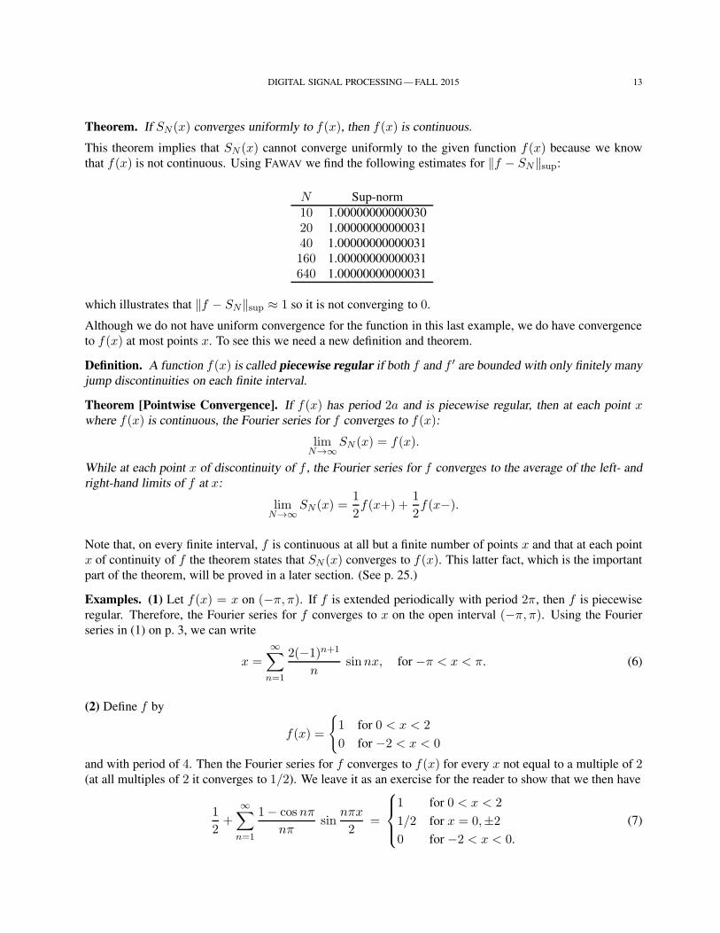
Theorem. If SN (x) converges uniformly to f(x), then f(x) is continuous.
This theorem implies that SN (x) cannot converge uniformly to the given function f(x) because we know
that f(x) is not continuous. Using FAWAV we find the following estimates for ‖f − SN‖sup:
N Sup-norm
10 1.00000000000030
20 1.00000000000031
40 1.00000000000031
160 1.00000000000031
640 1.00000000000031
which illustrates that ‖f − SN‖sup ≈ 1 so it is not converging to 0.
Although we do not have uniform convergence for the function in this last example, we do have convergence
to f(x) at most points x. To see this we need a new definition and theorem.
Definition. A function f(x) is called piecewise regular if both f and f ′ are bounded with only finitely many
jump discontinuities on each finite interval.
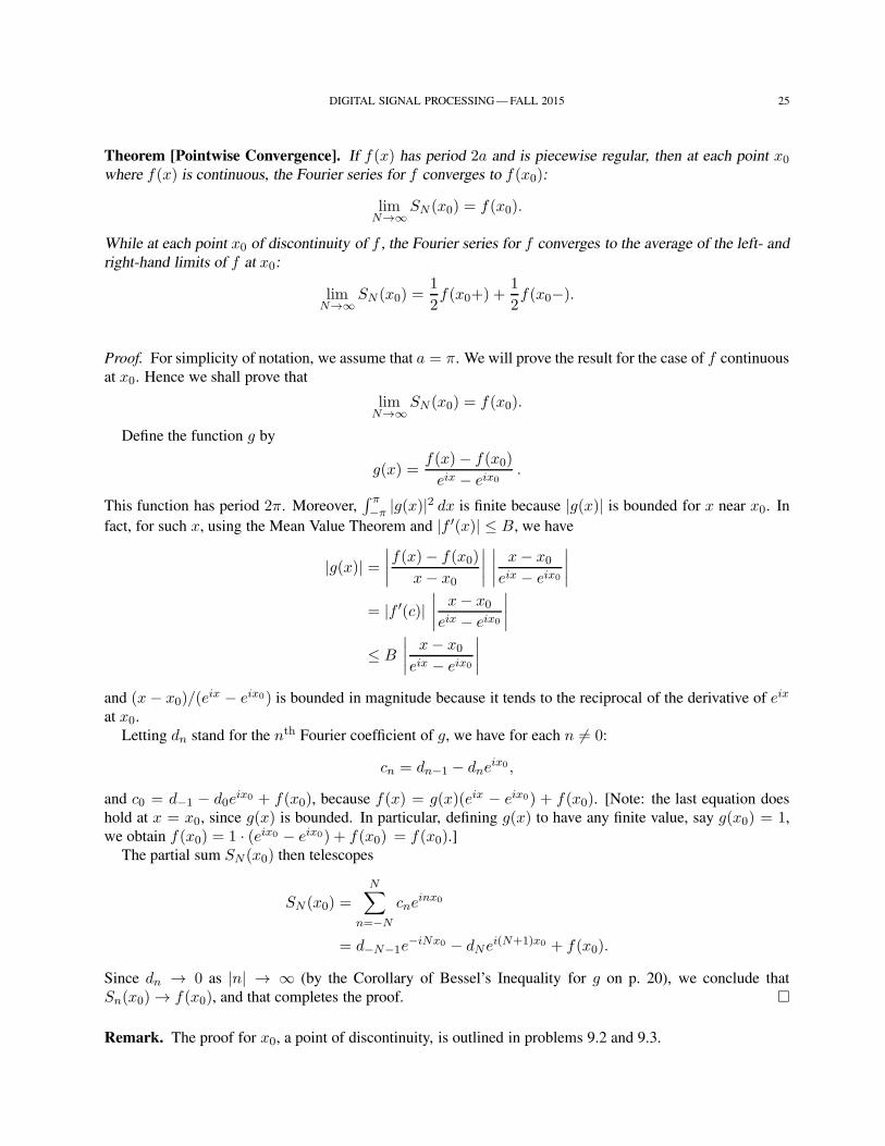
Theorem [Pointwise Convergence]. If f(x) has period 2a and is piecewise regular, then at each point xwhere f(x) is continuous, the Fourier series for f converges to f(x):
limN→∞
SN (x) = f(x).
While at each point x of discontinuity of f , the Fourier series for f converges to the average of the left- and
right-hand limits of f at x:
limN→∞
SN (x) =1
2f(x+) +
1
2f(x−).
Note that, on every finite interval, f is continuous at all but a finite number of points x and that at each point
x of continuity of f the theorem states that SN (x) converges to f(x). This latter fact, which is the important
part of the theorem, will be proved in a later section. (See p. 25.)
Examples. (1) Let f(x) = x on (−π, π). If f is extended periodically with period 2π, then f is piecewise
regular. Therefore, the Fourier series for f converges to x on the open interval (−π, π). Using the Fourier
series in (1) on p. 3, we can write
x =∞∑
n=1
2(−1)n+1
nsinnx, for −π < x < π. (6)
(2) Define f by
f(x) =
1 for 0 < x < 2
0 for −2 < x < 0
and with period of 4. Then the Fourier series for f converges to f(x) for every x not equal to a multiple of 2(at all multiples of 2 it converges to 1/2). We leave it as an exercise for the reader to show that we then have
1
2+
∞∑
n=1
1− cosnπ
nπsin
nπx
2=
1 for 0 < x < 2
1/2 for x = 0,±2
0 for −2 < x < 0.
(7)
14 DIGITAL SIGNAL PROCESSING — FALL 2015
Homework.
4.1S . For the following functions, state which have uniformly convergent Fourier series and which do not.
Briefly explain why.
(a) f(x) = |x| on [−π, π), period 2π.
(b) f(x) = ex on [−2, 2], period 4.
(c) f(x) = e−x2on [−3, 3), period 6.
(d) f(x) = sinx on [−π/2, π/2), period π.
(e) f(x) = | sinx| on [−π, π), period 2π.
4.2. For the following functions, state which have uniformly convergent Fourier series and which do not.
Briefly explain why.
(a) f(x) = x2 on [−3, 3), period 6.
(b) f(x) = cos x on [−π/3, π/3], period 2π/3.
(c) f(x) = x3 on [−1, 1), period 2.
(d) f(x) = |x| − x on [−2, 2), period 4.
(e) f(x) = sin e|x| on [−1, 1), period 2.
4.3. For f(x) = x+1 on [−1, 1), period 2, graph the function f(x) to which the Fourier series converges.
4.4. For f(x) = 3− x on [−2, 2), period 4, graph the function f(x) to which the Fourier series converges.
4.5S . Using FAWAV, compute the Fourier series partial sums SN for N = 10, 40, 160 for
f(x) =
1 for 0 < x < 1
−1 for −1 < x < 0
over the interval [−1, 1] using 8192 points. Find the sup-norms ‖|f − SN‖|sup over the interval [0.1, 0.9] for
these same values of N . What do you conjecture is happening?
4.6. Verify that (7) holds.
4.7. Prove that
π
2+
∞∑
k=0
4
π(2k + 1)2cos (2k + 1)x = π − |x|
holds for all x in the interval [−π, π].
5. COMPLEX EXPONENTIALS
Nowadays it is much more common to express Fourier series in complex exponential form. To do this, we
must first discuss the theory of complex exponentials.
Recall the MacLaurin expansion of et:
et =∞∑
n=0
tn
n!.
DIGITAL SIGNAL PROCESSING — FALL 2015 15
Substituting ix in place of t (where i =√−1) and rearranging terms yields
eix =
∞∑
n=0
inxn
n!
=∞∑
n=0(n even)
inxn
n!+
∞∑
n=1(n odd)
inxn
n!
=
∞∑
k=0
i2kx2k
(2k)!+
∞∑
k=0
i2k+1x2k+1
(2k + 1)!
=
∞∑
k=0
(−1)kx2k
(2k)!+ i
∞∑
k=0
(−1)kx2k+1
(2k + 1)!
= cos x+ i sinx
where we have used the MacLaurin expansions of cos x and sinx in the last step.
Thus we write
eix = cos x+ i sin x. (8)
We then also have einx = cosnx+ i sinnx. Furthermore, we have the following important identity
|eiθ| = 1 (9)
for all real values of θ. To see that (9) holds, we calculate |eiθ|2:
|eiθ|2 = eiθeiθ
= (cos θ + i sin θ)(cos θ − i sin θ)
= cos2 θ + sin2 θ
= 1.
Thus, |eiθ|2 = 1 so (9) holds.
We also make frequent use of
einxeimx = ei(n+m)x. (10)
To prove (10) we make use of the cosine and sine addition formulas:
einxeimx = (cosnx+ i sinnx)(cosmx+ i sinmx)
= (cosnx cosmx− sinnx sinmx) + i(sin nx cosmx+ sinmx cosnx)
= cos(n+m)x+ i sin(n+m)x
= ei(n+m)x.
Hence (10) holds.
The complex exponentials einx for all integers n (positive, negative and zero) will be used in the next
section to express Fourier series in complex exponential form. These exponentials can be differentiated:
(einx)′ = (cos nx+ i sinnx)′
= (cos nx)′ + i(sinnx)′
= −n sinnx+ in cosnx
= in(cosnx+ i sinnx)
= ineinx.
16 DIGITAL SIGNAL PROCESSING — FALL 2015
Thus (einx)′ = ineinx which follows the pattern we learned in calculus for differentiating exponentials.
We can also integrate: ∫einx dx =
1
ineinx +C
which checks by differentiation.
Homework.
5.1S . Prove that einx has period 2π/n.
5.2. Prove that einxe−inx = 1.
5.3S . Prove that (cos x+ i sinx)n = cosnx+ i sinnx.
5.4H . Find
∫ π/2
0xeinx dx.
5.5S . Using FAWAV graph the real and imaginary parts of f(x) = ei4x over the interval [−π, π].
5.6. Using FAWAV graph the real and imaginary parts of f(x) = 3ei6x over the interval [0, 2π].
6. COMPLEX EXPONENTIAL FORM OF FOURIER SERIES
We will express SN , and the Fourier series for a periodic function, in complex exponential form. To
simplify notation, we use period 2π. The case of a more general period is left to the reader.
For a function f of period 2π, its Fourier series partial sum SN is
SN (x) = c0 +N∑
n=1
(An cosnx+Bn sinnx) (11)
with
c0 =1
2π
∫ π
−πf(x) dx, An =
1
π
∫ π
−πf(x) cosnx dx, Bn =
1
π
∫ π
−πf(x) sinnx dx.
We make use of the following identities:
cos t =1
2eit +
1
2e−it , sin t =
i
2e−it − i
2eit (12)
to rewrite An and Bn as
An =1
2π
∫ π
−πf(x)einx dx+
1
2π
∫ π
−πf(x)e−inx dx
Bn =i
2π
∫ π
−πf(x)e−inx dx− i
2π
∫ π
−πf(x)einx dx.
Define
cn =1
2π
∫ π
−πf(x)e−inx dx, for n = 1, 2, 3, . . .
c−n =1
2π
∫ π
−πf(x)einx dx, for −n = −1,−2,−3, . . .
and we have
An = cn + c−n, Bn = icn − ic−n, for n = 1, 2, 3, . . .
DIGITAL SIGNAL PROCESSING — FALL 2015 17
Using these last equations, along with (12), we rewrite (11):
SN (x) = c0 +
N∑
n=1
[(cn + c−n)
(1
2einx +
1
2e−inx
)+ (icn − ic−n)
(i
2e−inx − i
2einx
)]
= c0 +N∑
n=1
(cneinx + c−ne
−inx)
=
N∑
n=−N
cneinx.
Thus, the complex exponential form for SN (x) is
SN (x) =
N∑
n=−N
cneinx , with cn =
1
2π
∫ π
−πf(x)e−inx dx for each integer n.
Letting N → ∞, we get the Fourier series for f(x):
∞∑
n=−∞cne
inx = limN→∞
N∑
n=−N
cneinx
with Fourier coefficients
cn =1
2π
∫ π
−πf(x)e−inx dx
for each integer n.
Example. Suppose f(x) = x on [−π, π) and has period 2π. Then we find that
c0 =1
2π
∫ π
−πx dx = 0
and for n 6= 0
cn =1
2π
∫ π
−πxe−inx dx
=1
2π
∫ π
−πx cosnx dx− i
2π
∫ π
−πx sinnx dx
=−i
π
∫ π
0x sinnx dx
=−i
π
(x− cosnx
n− 1
− sinnx
n2
)∣∣∣∣π
0
=i cosnπ
n
=i(−1)n
n.
The complex exponential form of the Fourier series is then
∞∑
n=−∞n 6=0
i(−1)n
neinx. (13)
18 DIGITAL SIGNAL PROCESSING — FALL 2015
Previously, we found a Fourier series for f(x) = x involving sine functions. See Equation (6) on p. 13.
We now show that these two series are, in fact, identical. Grouping together the positive and negative terms,
we find that∞∑
n=−∞n 6=0
i(−1)n
neinx =
∞∑
n=1
( i(−1)n
neinx +
i(−1)−n
−ne−inx
)
=
∞∑
n=1
i(−1)n
n
(einx − e−inx
)
=∞∑
n=1
2(−1)n+1
nsinnx
which is the Fourier series calculated previously for f(x).
Some typical waveforms in exponential terms. The complex exponential form for Fourier series allows
for simple expressions for the coefficients of waveforms typically used in sound synthesis. These typical
waveforms are (1) sawtooth waves, (2) shark tooth waves, and (3) square waves. Here are the formulas for
their Fourier coefficients:
sawtooth wave: cn ∝ 1
nfor all n 6= 0,
shark tooth wave: cn ∝ 1
n2for n odd,
square wave: cn ∝ 1
nfor n odd.
These waves are used a lot in sound synthesis applications.
Homework.
6.1S . Derive the complex exponential form of Fourier series for a function of period P = 2a.
6.2. Find the complex exponential forms for the Fourier series of the following functions.
(a)S f(x) = x2 on [−π, π), period 2π.
(b)S f(x) = ex on [−2, 2), period 4.
(c) f(x) = x3 on [−5, 5), period 10.
(d) f(x) = | sinx| on [−π, π), period 2π.
6.3S . Show that, for a real-valued function f(x) of period P , its Fourier coefficients cn satisfy
c−n = cn , n = 1, 2, 3, . . .
and that |c−n|2 = |cn|2.
6.4. By converting to real-forms, graph the Fourier series partial sums using the following coefficients:
(a) cn =5
nfor n = ±1,±2, . . . ,±21
(b) cn =5
n2for n = ±1,±3,±5, . . . ,±21
(c) cn =5
nfor n = ±1,±3,±5 . . . ,±21
DIGITAL SIGNAL PROCESSING — FALL 2015 19
7. ROOT MEAN SQUARE CONVERGENCE, PARSEVAL EQUATION
Let’s consider an example first. Let f(x) be defined by
f(x) =
1, if 0 < x < π
−1, if −π < x < 0.
As we saw previously, ‖f −SN‖sup does not converge to 0 as N → ∞. We want to define a single numerical
measure of the magnitude of difference between f and SN which does converge to 0. The required measure
is the root mean square of the difference, defined by
‖f − SN‖2 =√
1
2π
∫ π
−π|f(x)− SN (x)|2 dx .
(Note: mathematicians call this the 2-norm of the difference.) For the given function we use FAWAV to obtain
the following estimates (using 32768 points):3
N ‖f − SN‖210 0.20140 0.100160 0.050640 0.0242560 0.010
These results suggest that ‖f − SN‖2 → 0 as N → ∞.
Definition. We say that SN converges to f in root mean square (or in 2-norm) when
limN→∞
‖f − SN‖2 = 0.
Note: For period 2a,
‖f − SN‖2 =√
1
2a
∫ a
−a|f(x)− SN (x)|2 dx .
The following theorem shows that this notion of convergence applies to a wide variety of functions.
Theorem [Root Mean Square Convergence]. Suppose that∫ a−a |f(x)|2 dx is finite. Then the Fourier series
for f converges to f in root mean square.
Remark. The Root Mean Square Convergence Theorem applies to many more functions than either the
Uniform Convergence or Pointwise Convergence Theorems. For example, there are continuous functions for
which
|f(x0)− SN (x0)| → ∞for infinitely many points x0 (see Appendix A of Fourier Analysis). For these continuous functions, we have
failure of pointwise convergence at infinitely many points, and therefore also failure of uniform convergence,
but we still have root mean square convergence.
3To compute the root mean square, or 2-norm, difference ‖f − SN‖2 in FAWAV, you plot f and SN . Then select Analysis/Norm
difference from FAWAV’s menu, and select the option Power norm.
20 DIGITAL SIGNAL PROCESSING — FALL 2015
Theorem [Bessel’s Inequality]. For each N = 1, 2, 3, . . . , the Fourier coefficients of a function f satisfy
N∑
n=−N
|cn|2 ≤1
2a
∫ a
−a|f(x)|2 dx.
Proof. For simplicity of notation, assume that a = π. If the right side of the proposed inequality were ∞then the inequality would certainly hold. Therefore we assume that
∫ π−π |f(x)|2 dx is finite. We then have
0 ≤ 1
2π
∫ π
−π|f(x)− SN (x)|2 dx
=1
2π
∫ π
−π
(f(x)−
N∑
n=−N
cneinx) (
f(x)−N∑
m=−N
cme−imx)dx
=1
2π
∫ π
−π|f(x)|2 dx−
N∑
n=−N
cn1
2π
∫ π
−πf(x)e−inx dx
−N∑
m=−N
cm1
2π
∫ π
−πf(x)e−imx dx+
N∑
m=−N
N∑
n=−N
cncm1
2π
∫ π
−πeinxe−imx dx
=1
2π
∫ π
−π|f(x)|2 dx−
N∑
n=−N
|cn|2 −N∑
m=−N
|cm|2 +N∑
m=−N
|cm|2
=1
2π
∫ π
−π|f(x)|2 dx−
N∑
n=−N
|cn|2.
Thus,
N∑
n=−N
|cn|2 ≤1
2π
∫ π
−π|f(x)|2 dx
and the proof is complete.
Bessel’s Inequality can also be phrased as
N∑
n=−N
|cn|2 ≤ ‖f‖22.
Corollary. If∫ a−a |f(x)|2 dx is finite, then the Fourier coefficients cn for f satisfy
lim|n|→∞
cn = 0.
Proof. Letting N → ∞ in Bessel’s Inequality we see that
∞∑
n=−∞|cn|2 converges to a number less than or
equal to 12a
∫ a−a |f(x)|2 dx. Therefore, |cn|2 → 0 as |n| → ∞, hence cn → 0 as well.
DIGITAL SIGNAL PROCESSING — FALL 2015 21
Notice that we also showed in the proof of Bessel’s Inequality that
‖f − SN‖22 = ‖f‖22 −N∑
n=−N
|cn|2.
Combining this identity with the Root Mean Square Convergence Theorem we obtain the following theorem.
Theorem [Parseval’s Equality]. Given that∫ a−a |f(x)|2 dx is finite, we have
∞∑
n=−∞|cn|2 =
1
2a
∫ a
−a|f(x)|2 dx.
Homework.
7.1. For the following functions use FAWAV and 16384 points to compute ‖f − SN‖2 for N = 20, 80, 320,
and 1280.
(a) f(x) = x on [−2, 2).
(b) f(x) = ex on [−1, 1].
(c) f(x) = x2 on [−4, 4].
7.2S . Given the real form of Fourier series
c0 +
∞∑
n=1
(An cosnx+Bn sinnx
),
prove this version of Parseval’s Equality:
2c20 +
∞∑
n=1
(A2
n +B2n
)=
1
π
∫ π
−π|f(x)|2 dx.
[Hint: Use Parseval’s Equality as stated in the Theorem.]
7.3S . Prove that ‖f − SN‖2 is a decreasing sequence as N increases.
7.4S . Given that the Fourier series for f(x) = x on [−π, π) is
∞∑
n=−∞n 6=0
i(−1)n+1
neinx
use Parseval’s Equality to prove that∞∑
n=1
1
n2=
π2
6.
7.5S . Use the inequalityN∑
n=1
N∑
m=1
∣∣ anbm − ambn∣∣2 ≥ 0
to prove Cauchy’s inequality ∣∣∣∣∣N∑
n=1
anbn
∣∣∣∣∣
2
≤N∑
n=1
|an|2N∑
n=1
|bn|2.
22 DIGITAL SIGNAL PROCESSING — FALL 2015
0 660 1320 1980 2640−100
0
100
200
300
Frequency (Hz) Frequency (Hz)
Amp. Amp.
0 660 1320 1980 2640−50
0
50
100
150
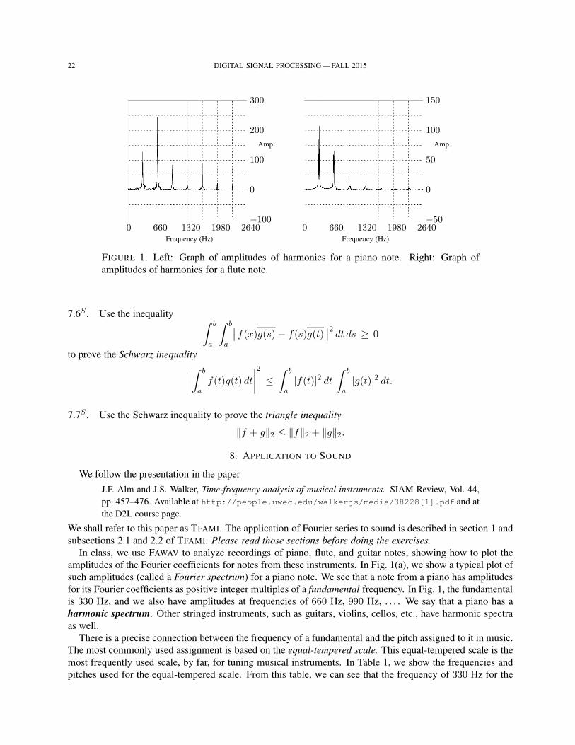
FIGURE 1. Left: Graph of amplitudes of harmonics for a piano note. Right: Graph of
amplitudes of harmonics for a flute note.
7.6S . Use the inequality ∫ b
a
∫ b
a
∣∣ f(x)g(s)− f(s)g(t)∣∣2 dt ds ≥ 0
to prove the Schwarz inequality
∣∣∣∣∫ b
af(t)g(t) dt
∣∣∣∣2
≤∫ b
a|f(t)|2 dt
∫ b
a|g(t)|2 dt.
7.7S . Use the Schwarz inequality to prove the triangle inequality
‖f + g‖2 ≤ ‖f‖2 + ‖g‖2.
8. APPLICATION TO SOUND
We follow the presentation in the paper
J.F. Alm and J.S. Walker, Time-frequency analysis of musical instruments. SIAM Review, Vol. 44,
pp. 457–476. Available at http://people.uwec.edu/walkerjs/media/38228[1].pdf and at
the D2L course page.
We shall refer to this paper as TFAMI. The application of Fourier series to sound is described in section 1 and
subsections 2.1 and 2.2 of TFAMI. Please read those sections before doing the exercises.
In class, we use FAWAV to analyze recordings of piano, flute, and guitar notes, showing how to plot the
amplitudes of the Fourier coefficients for notes from these instruments. In Fig. 1(a), we show a typical plot of
such amplitudes (called a Fourier spectrum) for a piano note. We see that a note from a piano has amplitudes
for its Fourier coefficients as positive integer multiples of a fundamental frequency. In Fig. 1, the fundamental
is 330 Hz, and we also have amplitudes at frequencies of 660 Hz, 990 Hz, . . . . We say that a piano has a
harmonic spectrum. Other stringed instruments, such as guitars, violins, cellos, etc., have harmonic spectra
as well.
There is a precise connection between the frequency of a fundamental and the pitch assigned to it in music.
The most commonly used assignment is based on the equal-tempered scale. This equal-tempered scale is the
most frequently used scale, by far, for tuning musical instruments. In Table 1, we show the frequencies and
pitches used for the equal-tempered scale. From this table, we can see that the frequency of 330 Hz for the
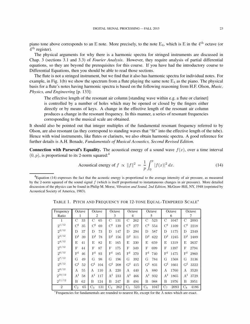
DIGITAL SIGNAL PROCESSING — FALL 2015 23
piano tone above corresponds to an E note. More precisely, to the note E4, which is E in the 4th octave (or
4th register).
The physical arguments for why there is a harmonic spectra for stringed instruments are discussed in
Chap. 3 (sections 3.1 and 3.3) of Fourier Analysis. However, they require analysis of partial differential
equations, so they are beyond the prerequisites for this course. If you have had the introductory course to
Differential Equations, then you should be able to read those sections.
The flute is not a stringed instrument, but we find that it also has harmonic spectra for individual notes. For
example, in Fig. 1(b) we show the spectrum from a flute playing the same note E4 as the piano. The physical
basis for a flute’s notes having harmonic spectra is based on the following reasoning from H.F. Olson, Music,
Physics, and Engineering [p. 133]:
The effective length of the resonant air column [standing wave within e.g. a flute or clarinet]
is controlled by a number of holes which may be opened or closed by the fingers either
directly or by means of keys. A change in the effective length of the resonant air column
produces a change in the resonant frequency. In this manner, a series of resonant frequencies
corresponding to the musical scale are obtained.
It should also be pointed out that integer multiples of the fundamental resonant frequency referred to by
Olson, are also resonant (as they correspond to standing waves that “fit” into the effective length of the tube).
Hence with wind instruments, like flutes or clarinets, we also obtain harmonic spectra. A good reference for
further details is A.H. Benade, Fundamentals of Musical Acoustics, Second Revised Edition.
Connection with Parseval’s Equality. The acoustical energy of a sound wave f(x), over a time interval
(0, p), is proportional to its 2-norm squared:4
Acoustical energy of f ∝ ‖f‖2 =1
p
∫ p
0|f(x)|2 dx. (14)
4Equation (14) expresses the fact that the acoustic energy is proportional to the average intensity of air pressure, as measured
by the 2-norm squared of the sound signal f (which is itself proportional to instantaneous changes in air pressure). More detailed
discussion of the physics can be found in Philip M. Morse, Vibration and Sound, 2nd Edition, McGraw-Hill, NY, 1948 (reprinted by
Acoustical Society of America, 1983).
TABLE 1. PITCH AND FREQUENCY FOR 12-TONE EQUAL-TEMPERED SCALE∗
Frequency Octave Octave Octave Octave Octave Octave Octave
Ratio 1 2 3 4 5 6 7
1 C 33 C 65 C 131 C 262 C 523 C 1047 C 2093
21/12 C♯ 35 C♯ 69 C♯ 139 C♯ 277 C♯ 554 C♯ 1109 C♯ 2218
22/12 D 37 D 73 D 147 D 294 D 587 D 1175 D 2349
23/12 D♯ 39 D♯ 78 D♯ 156 D♯ 311 D♯ 622 D♯ 1245 D♯ 2489
24/12 E 41 E 82 E 165 E 330 E 659 E 1319 E 2637
25/12 F 44 F 87 F 175 F 349 F 699 F 1397 F 2794
26/12 F♯ 46 F♯ 93 F♯ 185 F♯ 370 F♯ 740 F♯ 1475 F♯ 2960
27/12 G 49 G 98 G 196 G 392 G 784 G 1568 G 3136
28/12 G♯ 52 G♯ 104 G♯ 208 G♯ 415 G♯ 831 G♯ 1661 G♯ 3322
29/12 A 55 A 110 A 220 A 440 A 880 A 1760 A 3520
210/12 A♯ 58 A♯ 117 A♯ 233 A♯ 466 A♯ 932 A♯ 1865 A♯ 3729
211/12 B 62 B 124 B 247 B 494 B 988 B 1976 B 3951
2 C2 65 C3 131 C4 262 C5 523 C6 1047 C7 2093 C8 4186∗Frequencies for fundamentals are rounded to nearest Hz, except for the A notes which are exact.
24 DIGITAL SIGNAL PROCESSING — FALL 2015
Using this fact, we have that the acoustical energy of each Fourier series term, cnei2πnx/p, is proportional to
‖cnei2πnx/p‖2 =1
p
∫ p
0|cnei2πnx/p|2 dx
=1
p
∫ p
0|cn|2dx
= |cn|2.Therefore, Parseval’s Equality
∞∑
n=−∞|cn|2 = ‖f‖2
tells us that the acoustical energy of f(x) is equal to the sum of the acoustical energies of the individual terms
in its Fourier series. This illustrates the importance of Parseval’s Equality for acoustics. We shall see later
that it also plays a key role in the removing of random noise from sound signals.
Homework.
8.1. Show that formula (2.1) in TFAMI can be rewritten as (2.3).
8.2S . Using FAWAV, compute the spectrum of the recording Call (Jim).wav. Estimate the fundamen-
tal frequency ν0 and display the spectrum over the interval [0, 8ν0].
8.3. For the audio file Call back 2.wav, clip the sound “call”, estimate its fundamental frequency
ν0, and display its spectrum over the interval [0, 8ν0]. How does this spectrum compare with the one in Exer-
cise 8.2?
8.4S . For the audio file Chong’s ‘Bait’.wav, estimate the fundamental frequency ν0, and display its
spectrum over the interval [0, 8ν0].
8.5. For the audio file Sara’s ‘Bait’.wav, estimate the fundamental frequency ν0, and display its
spectrum over the interval [0, 8ν0]. How does this analysis compare with the previous exercise?
8.6S . Using FAWAV, plot the function
20000cos(2pi vx) \v = 440
over the interval [0, 1], using 8192 points, and plot its spectrum. Play the sound at a sampling rate of 8192
samples per second and a bit rate of 16 bits. Repeat this work for the second function
20000bell[2(x-1/2)]cos(2pi vx) \v = 440
What is the difference between the sounds for the two functions? Can you explain why there is a difference?
8.7. Using FAWAV, plot the function
5000bell(2(x-1/2))[4cos(2pi ax)+2cos(2pi bx)+cos(2pi cx)]
\a=440\b=880\c=1340
over the interval [0, 1] using 8192 points, and plot its spectrum (within a suitably chosen window). Play the
sound for this signal at a sampling rate of 8192 samples/sec and bit rate of 16 bits. What does it sound like?
9. PROOFS OF CONVERGENCE THEOREMS (OPTIONAL)
In this optional section we prove the Pointwise Convergence Theorem, the Uniform Convergence Theorem,
and the Root Mean Square Convergence Theorem.
DIGITAL SIGNAL PROCESSING — FALL 2015 25
Theorem [Pointwise Convergence]. If f(x) has period 2a and is piecewise regular, then at each point x0where f(x) is continuous, the Fourier series for f converges to f(x0):
limN→∞
SN (x0) = f(x0).
While at each point x0 of discontinuity of f , the Fourier series for f converges to the average of the left- and
right-hand limits of f at x0:
limN→∞
SN (x0) =1
2f(x0+) +
1
2f(x0−).
Proof. For simplicity of notation, we assume that a = π. We will prove the result for the case of f continuous
at x0. Hence we shall prove that
limN→∞
SN (x0) = f(x0).
Define the function g by
g(x) =f(x)− f(x0)
eix − eix0.
This function has period 2π. Moreover,∫ π−π |g(x)|2 dx is finite because |g(x)| is bounded for x near x0. In
fact, for such x, using the Mean Value Theorem and |f ′(x)| ≤ B, we have
|g(x)| =∣∣∣∣f(x)− f(x0)
x− x0
∣∣∣∣∣∣∣∣
x− x0eix − eix0
∣∣∣∣
= |f ′(c)|∣∣∣∣
x− x0eix − eix0
∣∣∣∣
≤ B
∣∣∣∣x− x0
eix − eix0
∣∣∣∣
and (x− x0)/(eix − eix0) is bounded in magnitude because it tends to the reciprocal of the derivative of eix
at x0.
Letting dn stand for the nth Fourier coefficient of g, we have for each n 6= 0:
cn = dn−1 − dneix0 ,
and c0 = d−1 − d0eix0 + f(x0), because f(x) = g(x)(eix − eix0) + f(x0). [Note: the last equation does
hold at x = x0, since g(x) is bounded. In particular, defining g(x) to have any finite value, say g(x0) = 1,
we obtain f(x0) = 1 · (eix0 − eix0) + f(x0) = f(x0).]The partial sum SN (x0) then telescopes
SN (x0) =
N∑
n=−N
cneinx0
= d−N−1e−iNx0 − dNei(N+1)x0 + f(x0).
Since dn → 0 as |n| → ∞ (by the Corollary of Bessel’s Inequality for g on p. 20), we conclude that
Sn(x0) → f(x0), and that completes the proof.
Remark. The proof for x0, a point of discontinuity, is outlined in problems 9.2 and 9.3.
26 DIGITAL SIGNAL PROCESSING — FALL 2015
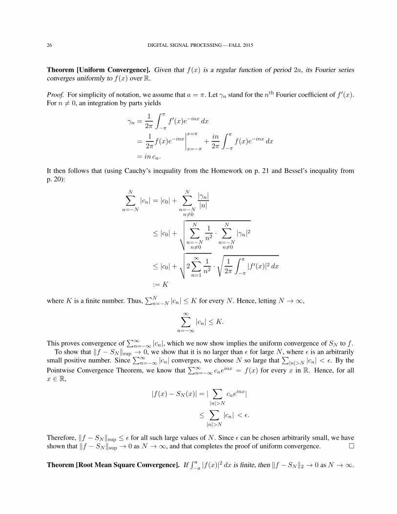
Theorem [Uniform Convergence]. Given that f(x) is a regular function of period 2a, its Fourier series
converges uniformly to f(x) over R.
Proof. For simplicity of notation, we assume that a = π. Let γn stand for the nth Fourier coefficient of f ′(x).For n 6= 0, an integration by parts yields
γn =1
2π
∫ π
−πf ′(x)e−inx dx
=1
2πf(x)e−inx
∣∣∣∣x=π
x=−π
+in
2π
∫ π
−πf(x)e−inx dx
= in cn.
It then follows that (using Cauchy’s inequality from the Homework on p. 21 and Bessel’s inequality from
p. 20):
N∑
n=−N
|cn| = |c0|+N∑
n=−Nn 6=0
|γn||n|
≤ |c0|+
√√√√√N∑
n=−Nn 6=0
1
n2·
N∑
n=−Nn 6=0
|γn|2
≤ |c0|+
√√√√2∞∑
n=1
1
n2·√
1
2π
∫ π
−π|f ′(x)|2 dx
:= K
where K is a finite number. Thus,∑N
n=−N |cn| ≤ K for every N . Hence, letting N → ∞,
∞∑
n=−∞|cn| ≤ K.
This proves convergence of∑∞
n=−∞ |cn|, which we now show implies the uniform convergence of SN to f .
To show that ‖f − SN‖sup → 0, we show that it is no larger than ǫ for large N , where ǫ is an arbitrarily
small positive number. Since∑∞
n=−∞ |cn| converges, we choose N so large that∑
|n|>N |cn| < ǫ. By the
Pointwise Convergence Theorem, we know that∑∞
n=−∞ cneinx = f(x) for every x in R. Hence, for all
x ∈ R,
|f(x)− SN (x)| = |∑
|n|>N
cneinx|
≤∑
|n|>N
|cn| < ǫ.
Therefore, ‖f − SN‖sup ≤ ǫ for all such large values of N . Since ǫ can be chosen arbitrarily small, we have
shown that ‖f − SN‖sup → 0 as N → ∞, and that completes the proof of uniform convergence.
Theorem [Root Mean Square Convergence]. If∫ a−a |f(x)|2 dx is finite, then ‖f − SN‖2 → 0 as N → ∞.
DIGITAL SIGNAL PROCESSING — FALL 2015 27
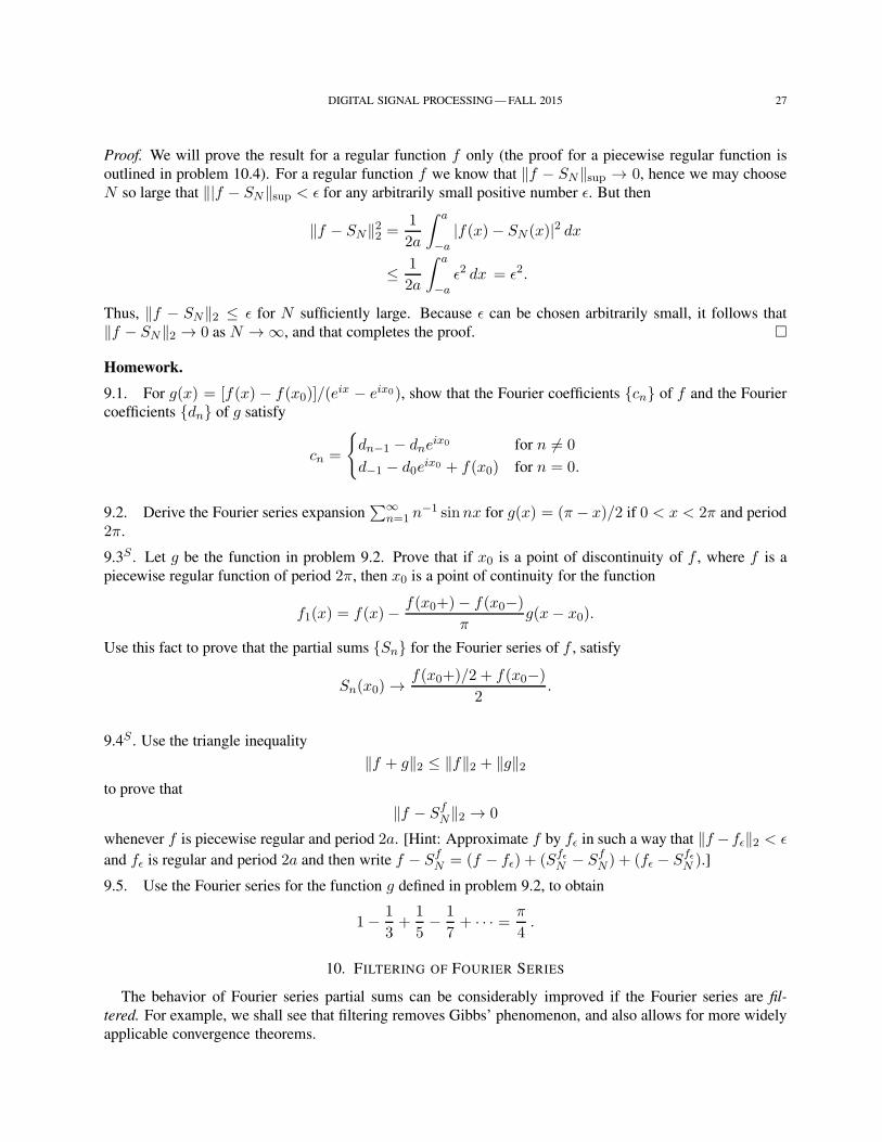
Proof. We will prove the result for a regular function f only (the proof for a piecewise regular function is
outlined in problem 10.4). For a regular function f we know that ‖f − SN‖sup → 0, hence we may choose
N so large that ‖|f − SN‖sup < ǫ for any arbitrarily small positive number ǫ. But then
‖f − SN‖22 =1
2a
∫ a
−a|f(x)− SN (x)|2 dx
≤ 1
2a
∫ a
−aǫ2 dx = ǫ2.
Thus, ‖f − SN‖2 ≤ ǫ for N sufficiently large. Because ǫ can be chosen arbitrarily small, it follows that
‖f − SN‖2 → 0 as N → ∞, and that completes the proof.
Homework.
9.1. For g(x) = [f(x) − f(x0)]/(eix − eix0), show that the Fourier coefficients cn of f and the Fourier
coefficients dn of g satisfy
cn =
dn−1 − dne
ix0 for n 6= 0
d−1 − d0eix0 + f(x0) for n = 0.
9.2. Derive the Fourier series expansion∑∞
n=1 n−1 sinnx for g(x) = (π − x)/2 if 0 < x < 2π and period
2π.
9.3S . Let g be the function in problem 9.2. Prove that if x0 is a point of discontinuity of f , where f is a
piecewise regular function of period 2π, then x0 is a point of continuity for the function
f1(x) = f(x)− f(x0+)− f(x0−)
πg(x− x0).
Use this fact to prove that the partial sums Sn for the Fourier series of f , satisfy
Sn(x0) →f(x0+)/2 + f(x0−)
2.
9.4S . Use the triangle inequality
‖f + g‖2 ≤ ‖f‖2 + ‖g‖2to prove that
‖f − SfN‖2 → 0
whenever f is piecewise regular and period 2a. [Hint: Approximate f by fǫ in such a way that ‖f − fǫ‖2 < ǫ
and fǫ is regular and period 2a and then write f − SfN = (f − fǫ) + (Sfǫ
N − SfN ) + (fǫ − Sfǫ
N ).]
9.5. Use the Fourier series for the function g defined in problem 9.2, to obtain
1− 1
3+
1
5− 1
7+ · · · = π
4.
10. FILTERING OF FOURIER SERIES
The behavior of Fourier series partial sums can be considerably improved if the Fourier series are fil-
tered. For example, we shall see that filtering removes Gibbs’ phenomenon, and also allows for more widely
applicable convergence theorems.
28 DIGITAL SIGNAL PROCESSING — FALL 2015
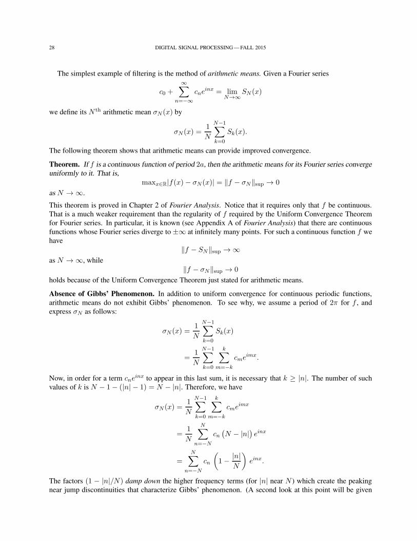
The simplest example of filtering is the method of arithmetic means. Given a Fourier series
c0 +
∞∑
n=−∞cne
inx = limN→∞
SN (x)
we define its N th arithmetic mean σN (x) by
σN (x) =1
N
N−1∑
k=0
Sk(x).
The following theorem shows that arithmetic means can provide improved convergence.
Theorem. If f is a continuous function of period 2a, then the arithmetic means for its Fourier series converge
uniformly to it. That is,
maxx∈R|f(x)− σN (x)| = ‖f − σN‖sup → 0
as N → ∞.
This theorem is proved in Chapter 2 of Fourier Analysis. Notice that it requires only that f be continuous.
That is a much weaker requirement than the regularity of f required by the Uniform Convergence Theorem
for Fourier series. In particular, it is known (see Appendix A of Fourier Analysis) that there are continuous
functions whose Fourier series diverge to ±∞ at infinitely many points. For such a continuous function f we
have
‖f − SN‖sup → ∞as N → ∞, while
‖f − σN‖sup → 0
holds because of the Uniform Convergence Theorem just stated for arithmetic means.
Absence of Gibbs’ Phenomenon. In addition to uniform convergence for continuous periodic functions,
arithmetic means do not exhibit Gibbs’ phenomenon. To see why, we assume a period of 2π for f , and
express σN as follows:
σN (x) =1
N
N−1∑
k=0
Sk(x)
=1
N
N−1∑
k=0
k∑
m=−k
cmeimx.
Now, in order for a term cneinx to appear in this last sum, it is necessary that k ≥ |n|. The number of such
values of k is N − 1− (|n| − 1) = N − |n|. Therefore, we have
σN (x) =1
N
N−1∑
k=0
k∑
m=−k
cmeimx
=1
N
N∑
n=−N
cn(N − |n|
)einx
=N∑
n=−N
cn
(1− |n|
N
)einx.
The factors (1 − |n|/N) damp down the higher frequency terms (for |n| near N ) which create the peaking
near jump discontinuities that characterize Gibbs’ phenomenon. (A second look at this point will be given
DIGITAL SIGNAL PROCESSING — FALL 2015 29
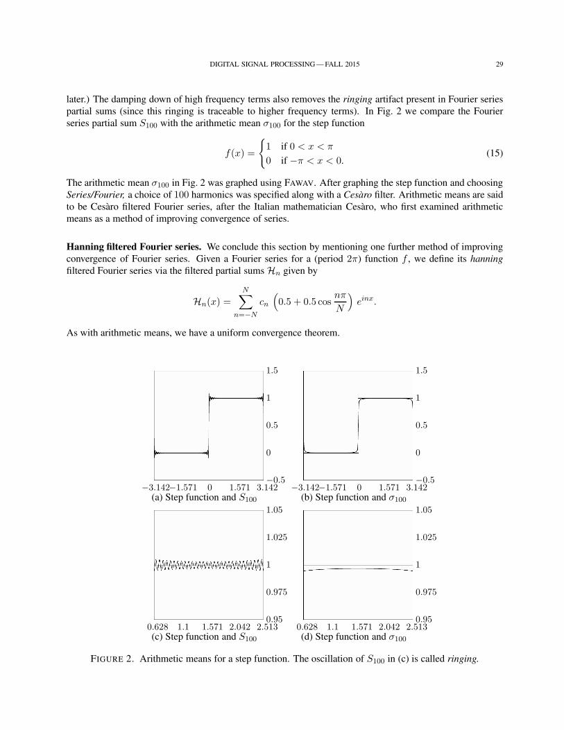
later.) The damping down of high frequency terms also removes the ringing artifact present in Fourier series
partial sums (since this ringing is traceable to higher frequency terms). In Fig. 2 we compare the Fourier
series partial sum S100 with the arithmetic mean σ100 for the step function
f(x) =
1 if 0 < x < π
0 if −π < x < 0.(15)
The arithmetic mean σ100 in Fig. 2 was graphed using FAWAV. After graphing the step function and choosing
Series/Fourier, a choice of 100 harmonics was specified along with a Cesaro filter. Arithmetic means are said
to be Cesaro filtered Fourier series, after the Italian mathematician Cesaro, who first examined arithmetic
means as a method of improving convergence of series.
Hanning filtered Fourier series. We conclude this section by mentioning one further method of improving
convergence of Fourier series. Given a Fourier series for a (period 2π) function f , we define its hanning
filtered Fourier series via the filtered partial sums Hn given by
Hn(x) =
N∑
n=−N
cn
(0.5 + 0.5 cos
nπ
N
)einx.
As with arithmetic means, we have a uniform convergence theorem.
−3.142−1.571 0 1.571 3.142−0.5
0
0.5
1
1.5
(a) Step function and S100
−3.142−1.571 0 1.571 3.142−0.5
0
0.5
1
1.5
(b) Step function and σ100
0.628 1.1 1.571 2.042 2.5130.95
0.975
1
1.025
1.05
(c) Step function and S100
0.628 1.1 1.571 2.042 2.5130.95
0.975
1
1.025
1.05
(d) Step function and σ100
FIGURE 2. Arithmetic means for a step function. The oscillation of S100 in (c) is called ringing.
30 DIGITAL SIGNAL PROCESSING — FALL 2015
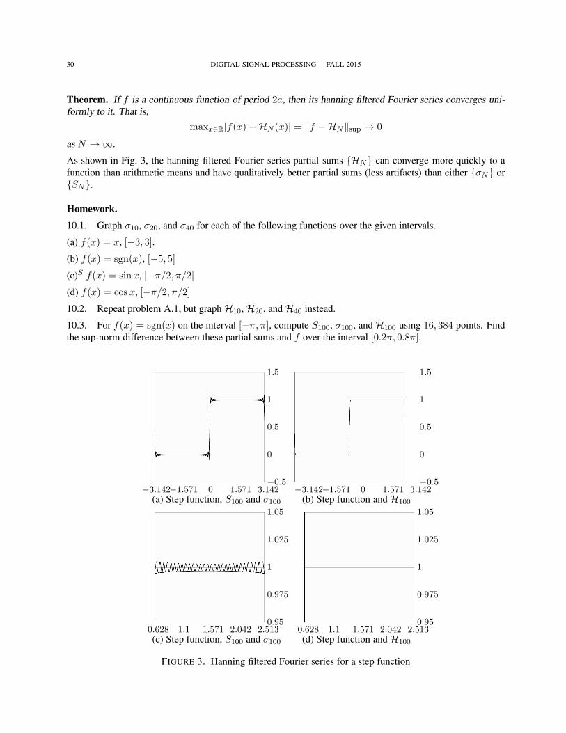
Theorem. If f is a continuous function of period 2a, then its hanning filtered Fourier series converges uni-
formly to it. That is,
maxx∈R|f(x)−HN (x)| = ‖f −HN‖sup → 0
as N → ∞.
As shown in Fig. 3, the hanning filtered Fourier series partial sums HN can converge more quickly to a
function than arithmetic means and have qualitatively better partial sums (less artifacts) than either σN or
SN.
Homework.
10.1. Graph σ10, σ20, and σ40 for each of the following functions over the given intervals.
(a) f(x) = x, [−3, 3].
(b) f(x) = sgn(x), [−5, 5]
(c)S f(x) = sinx, [−π/2, π/2]
(d) f(x) = cos x, [−π/2, π/2]
10.2. Repeat problem A.1, but graph H10, H20, and H40 instead.
10.3. For f(x) = sgn(x) on the interval [−π, π], compute S100, σ100, and H100 using 16, 384 points. Find
the sup-norm difference between these partial sums and f over the interval [0.2π, 0.8π].
−3.142−1.571 0 1.571 3.142−0.5
0
0.5
1
1.5
(a) Step function, S100 and σ100−3.142−1.571 0 1.571 3.142
−0.5
0
0.5
1
1.5
(b) Step function and H100
0.628 1.1 1.571 2.042 2.5130.95
0.975
1
1.025
1.05
(c) Step function, S100 and σ1000.628 1.1 1.571 2.042 2.513
0.95
0.975
1
1.025
1.05
(d) Step function and H100
FIGURE 3. Hanning filtered Fourier series for a step function
DIGITAL SIGNAL PROCESSING — FALL 2015 31
11. CONVOLUTION AND KERNELS
The behavior of partial sums, filtered and unfiltered, can be analyzed by expressing them as periodic
convolutions.
Definition. Given two functions of period 2a, their periodic convolution is defined by
(f ∗ g)(x) = 1
2a
∫ a
−af(t)g(x− t) dt.
As an example of where periodic convolution occurs, consider the partial sum SN for a function f :
SN (x) =
N∑
n=−N
cneinx, cn =
1
2π
∫ π
−πf(t)e−int dt.
Replacing each cn by its integral formula and performing algebra with integrals we obtain
SN (x) =N∑
n=−N
1
2π
∫ π
−πf(t)e−int dt einx
=1
2π
∫ π
−π
N∑
n=−N
ein(x−t) f(t) dt.
Defining the Dirichlet kernel DN by
DN (x) =
N∑
n=−N
einx (16)
we obtain the convolution form for SN :
SN (x) =1
2π
∫ π
−πf(t)DN (x− t) dt = (f ∗DN )(x).
We leave it as an exercise for the reader to check that Dirichlet’s kernel satisfies the following identity
1
2π
∫ π
−πDN (x) dx = 1 (17)
for each N .
To see how the convolution form SN = f ∗DN helps us to understand the behavior of the Fourier series
partial sums, we need the following identity
DN (x) =sin (N + 1/2)x
sin(x/2)(18)
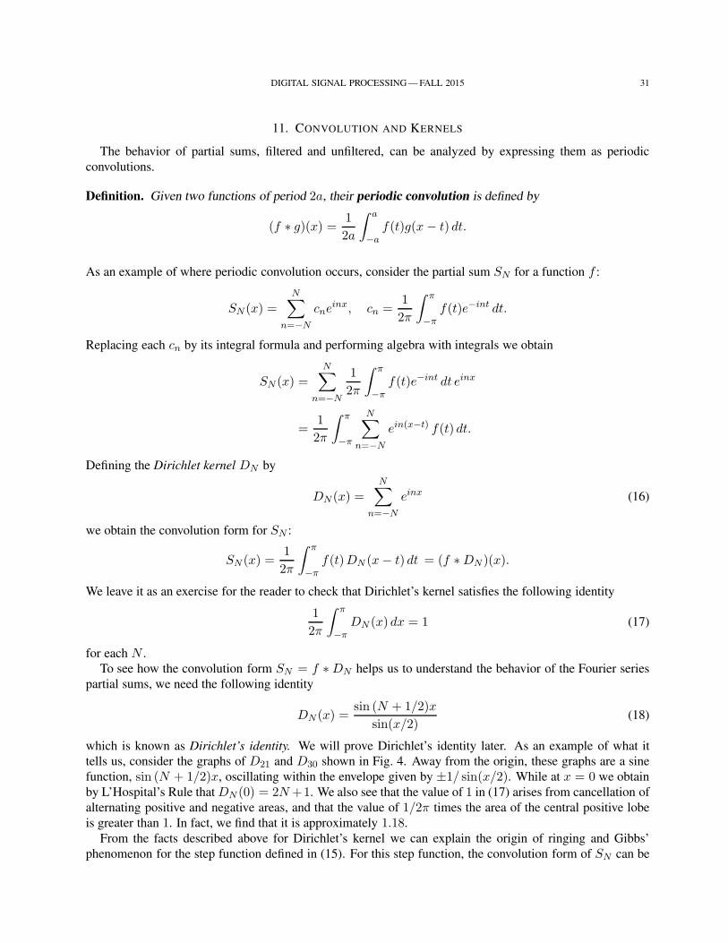
which is known as Dirichlet’s identity. We will prove Dirichlet’s identity later. As an example of what it
tells us, consider the graphs of D21 and D30 shown in Fig. 4. Away from the origin, these graphs are a sine
function, sin (N + 1/2)x, oscillating within the envelope given by ±1/ sin(x/2). While at x = 0 we obtain
by L’Hospital’s Rule that DN (0) = 2N+1. We also see that the value of 1 in (17) arises from cancellation of
alternating positive and negative areas, and that the value of 1/2π times the area of the central positive lobe
is greater than 1. In fact, we find that it is approximately 1.18.
From the facts described above for Dirichlet’s kernel we can explain the origin of ringing and Gibbs’
phenomenon for the step function defined in (15). For this step function, the convolution form of SN can be
32 DIGITAL SIGNAL PROCESSING — FALL 2015
−3.142−1.571 0 1.571 3.142−20
0
20
40
60
Graph of D21
−3.142−1.571 0 1.571 3.142−25
0
25
50
75
Graph of D30
FIGURE 4. Instances of Dirichlet’s kernel.
rewritten (using the evenness of DN ) as
SN (x) =1
2π
∫ π
0DN (t− x) dt.
As x ranges from −π to π, this formula shows that SN (x) is proportional to the signed area from 0 to π of
DN shifted so that its peak is above x. By examining Fig. 4 which show typical graphs for DN , it is easy
to see why there is ringing in the partial sums SN for the square wave—the very prominent oscillations of
DN induce the ringing oscillations in SN . Gibbs’ phenomenon is a bit more subtle, but also results from this
last expression for SN . For example, when x is slightly to the right of 0, the cental lobe in DN (t− x) is the
dominant contributor to this integral for SN , resulting in a spike which overshoots the value of 1 by about
9%.
There is a similar convolution form for arithmetic means. In fact, using the definition of σN and linearity
of integration we obtain
σN (x) =1
N
N−1∑
k=0
1
2π
∫ π
−πf(t)Dk(x− t) dt
=1
2π
∫ π
−πf(t)
1
N
N−1∑
k=0
Dk(x− t) dt.
Defining the Fejer kernel FN by
FN (x) =1
N
N−1∑
k=0
Dk(x)
we have the convolution form for σN (x):
σN (x) =1
2π
∫ π
−πf(t)FN (x− t) dt.
We will show a bit later that FN satisfies the following identity:
FN (x) =1
N
(sin Nx/2
sinx/2
)2
. (19)
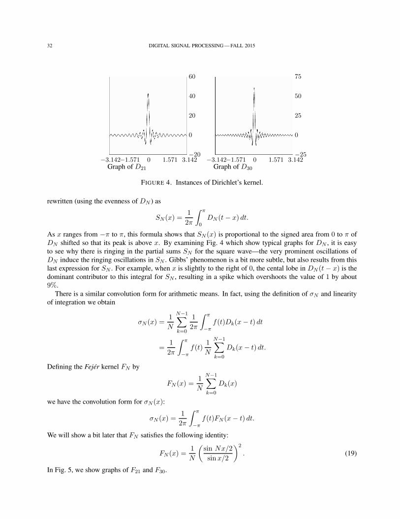
In Fig. 5, we show graphs of F21 and F30.
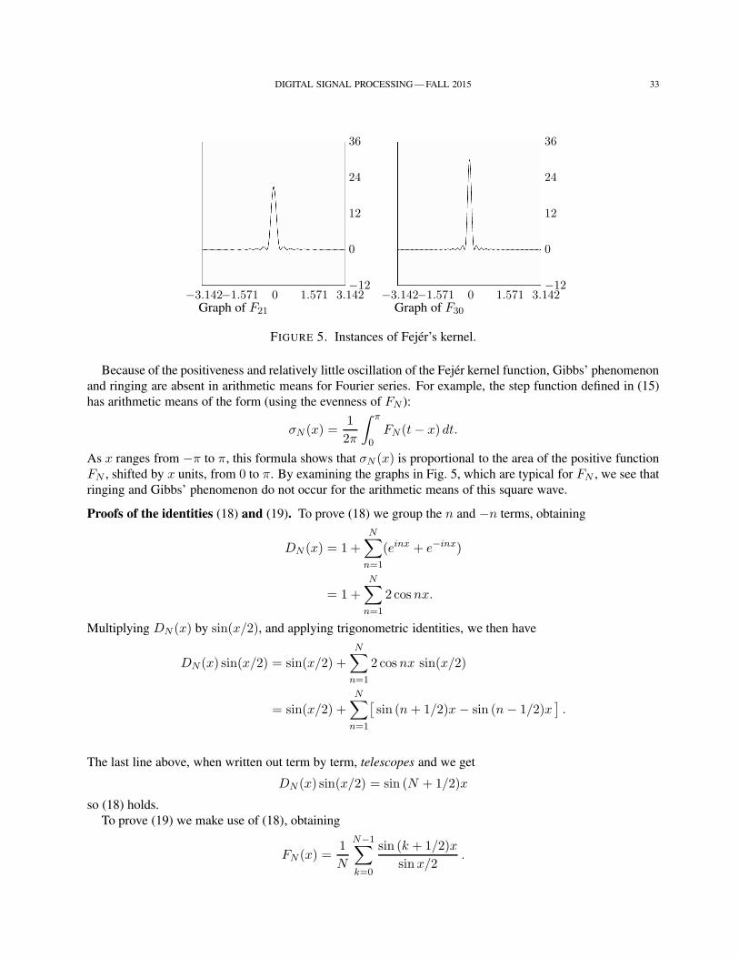
DIGITAL SIGNAL PROCESSING — FALL 2015 33
−3.142−1.571 0 1.571 3.142−12
0
12
24
36
Graph of F21
−3.142−1.571 0 1.571 3.142−12
0
12
24
36
Graph of F30
FIGURE 5. Instances of Fejer’s kernel.
Because of the positiveness and relatively little oscillation of the Fejer kernel function, Gibbs’ phenomenon
and ringing are absent in arithmetic means for Fourier series. For example, the step function defined in (15)
has arithmetic means of the form (using the evenness of FN ):
σN (x) =1
2π
∫ π
0FN (t− x) dt.
As x ranges from −π to π, this formula shows that σN (x) is proportional to the area of the positive function
FN , shifted by x units, from 0 to π. By examining the graphs in Fig. 5, which are typical for FN , we see that
ringing and Gibbs’ phenomenon do not occur for the arithmetic means of this square wave.
Proofs of the identities (18) and (19). To prove (18) we group the n and −n terms, obtaining
DN (x) = 1 +
N∑
n=1
(einx + e−inx)
= 1 +N∑
n=1
2 cosnx.
Multiplying DN (x) by sin(x/2), and applying trigonometric identities, we then have
DN (x) sin(x/2) = sin(x/2) +
N∑
n=1
2 cosnx sin(x/2)
= sin(x/2) +
N∑
n=1
[sin (n+ 1/2)x − sin (n− 1/2)x
].
The last line above, when written out term by term, telescopes and we get
DN (x) sin(x/2) = sin (N + 1/2)x
so (18) holds.
To prove (19) we make use of (18), obtaining
FN (x) =1
N
N−1∑
k=0
sin (k + 1/2)x
sinx/2.
34 DIGITAL SIGNAL PROCESSING — FALL 2015
Multiplying the equation above by sin2(x/2) we have (by trigonometric identities and telescoping):
FN (x) sin2(x/2) =1
N
N−1∑
k=0
sin (k + 1/2)x sin(x/2)
=1
2N
N−1∑
k=0
[cos kx− cos(k + 1)x]
=1
2N(1− cos Nx)
By the trigonometric identity 1− cos θ = 2 sin2(θ/2), we then have
FN (x) sin2(x/2) =1
Nsin2(Nx/2)
so (19) holds.
Homework.
11.1S . Prove (17). [Note: Use the definition of DN (x) as
N∑
n=−N
einx.]
11.2. By summing
N∑
n=0
einx and
N∑
n=1
e−inx as finite geometric series, provide a second proof of (18).
11.3. Using DN (x) = 1 +
N∑
n=1
2 cosnx and trigonometric identities, show that HN (x) = (f ∗ HN )(x)
where the hanning kernel HN satisfies
HN(x) = 0.5DN (x) + 0.25DN
(x− π
N
)+ 0.25DN
(x+
π
N
).
11.4H . Use FAWAV, along with the formula from problem 11.3 and the fact that DN (x) = 1+∑N
n=1 2 cosnxto graph H21 and H30. From the form of these graphs, do you expect ringing or Gibbs’ phenomenon for the
hanning filtered partial sums HN of the step function defined in (15)?
PART 2. DISCRETE FOURIER ANALYSIS
12. DISCRETE FOURIER TRANSFORMS (DFTS)
The discrete form of Fourier analysis is based on DFTs that are obtained by discretizing Fourier series.
Given a complex exponential Fourier series for a signal f(t)
∞∑
n=−∞cn e
i2πnt/Ω, cn =1
Ω
∫ Ω
0f(t)e−i2πnt/Ω dt
DIGITAL SIGNAL PROCESSING — FALL 2015 35
we approximate cn by a Riemann sum with N equally spaced subintervals of [0,Ω]. That is, we use tk =kΩ/N and ∆t = Ω/N and get
cn ≈ 1
Ω
N−1∑
k=0
f(tk)e−i2πntk/Ω
Ω
N
=1
N
N−1∑
k=0
f(tk)e−i2πnk/N .
Definition. Given a sequence of N numbers (fk)N−1k=0 = (f0, f1, . . . , fN−1), we define its N -point DFT
Fn by
Fn =N−1∑
k=0
fke−i2πnk/N .
Thus, we have
cn ≈ 1
NFn.
Note: The sound spectra computed previously were obtained using the approximation |cn| ≈ |Fn|/N . In
other words, a DFT Fn was computed for fk = f(tk) and then |Fn|/N was plotted as an approxi-
mation to the spectrum |cn|.
Examples. (1) We compute the 8-point DFT of (fk) = (1, 1, 1, 0, 0, 0, 1, 1). We have
Fn = 1 e0 + 1 e−i2nπ/8 + 1 e−i4nπ/8 + 1 e−i12nπ/8 + 1 e−i14nπ/8
= 1 + (e−i2nπ/8 + e−i16nπ/8+i2nπ/8) + (e−i4nπ/8 + e−i16nπ/8+i4nπ/8)
= 1 + (e−i2nπ/8 + e+i2nπ/8) + (e−i4nπ/8 + e+i4nπ/8)
= 1 + 2 cos(nπ/4) + 2 cos(nπ/2).
(2) We compute the N -point DFT of (ekc)N−1k=0 . We have
Fn =
N−1∑
k=0
ekc e−i2πkn/N
=
N−1∑
k=0
ek(c−i2πn/N)
= 1 + ec−i2πn/N + (ec−i2πn/N )2 + · · ·+ (ec−i2πn/N )N−1
=1− (ec−i2πn/N )N
1− ec−i2πn/N
where we used the well-known formula for the sum of a finite geometric series:
a+ ar + ar2 + · · ·+ arN−1 =a− arN
1− r.
Since (ec−i2πn/N )N = eNce−i2πn = eNc, we obtain
Fn =1− eNc
1− ec−i2πn/N.
36 DIGITAL SIGNAL PROCESSING — FALL 2015
Properties of DFTs. There are four important properties of the DFT. We use the notation fkDFT−→ Fn to
denote the operation of an N -point DFT.
1. Linearity: For constants α and β,
αfk + βgkDFT−→ αFn + βGn.
2. Periodicity: Fn+N = Fn for all n.
3. Inversion: For each k = 0, 1, . . . , N − 1, we have
fk =1
N
N−1∑
n=0
Fn e+i2πkn/N .
4. Parseval’s Equality:
N−1∑
k=0
|fk|2 =1
N
N−1∑
n=0
|Fn|2.
Proofs. 1. The DFT of αfk + βgk is
N−1∑
k=0
(αfk + βgk)e−i2πkn/N = α
N−1∑
k=0
fke−i2πkn/N + β
N−1∑
k=0
gke−i2πkn/N
= αFn + βGn.
2. We have
Fn+N =N−1∑
k=0
fke−i2πk(n+N)/N
=
N−1∑
k=0
fke−i2πnk/Ne−i2πk
=
N−1∑
k=0
fke−i2πnk/N · 1
= Fn.
3. Fix a value of k from 0 to N − 1. We then have
1
N
N−1∑
n=0
Fne+i2πkn/N =
N−1∑
n=0
1
N
N−1∑
ℓ=0
fℓ e−i2πℓn/N e+i2πkn/N
=
N−1∑
ℓ=0
fℓ
(1
N
N−1∑
n=0
e−i2πℓn/N e+i2πkn/N
)
=
N−1∑
ℓ=0
fℓ
(1
N
N−1∑
n=0
ei2π(k−ℓ)n/N
).
We now simplify the innermost sum in the last line above. If ℓ = k, then we have
N−1∑
n=0
ei2π(k−ℓ)n/N =N−1∑
n=0
e0 = N.
DIGITAL SIGNAL PROCESSING — FALL 2015 37
If ℓ 6= k, then we have (using a geometric series sum):
N−1∑
n=0
ei2π(k−ℓ)n/N =
N−1∑
n=0
(ei2π(k−ℓ)/N )n
=1− (ei2π(k−ℓ)/N )N
1− ei2π(k−ℓ)/N
=1− ei2π(k−ℓ)
1− ei2π(k−ℓ)/N
=1− 1
1− ei2π(k−ℓ)/N
= 0.
Therefore, we have
1
N
N−1∑
n=0
Fne+i2πkn/N =
N−1∑
ℓ=0
fℓ
(1
N
N−1∑
n=0
ei2π(k−ℓ)n/N
)
=∑
ℓ 6=k
fℓ
(1
N
N−1∑
n=0
ei2π(k−ℓ)n/N
)+ fk
(1
N
N−1∑
k=0
e0
)
=∑
ℓ 6=k
fℓ · 0 + fk · 1
= fk
and inversion is proved. We leave the proof of property 4 as an exercise.
Homework.
12.1. Compute the 8-point DFT of (fk) = (1 1 1 1 0 1 1 1).
12.2S . Compute the 16-point DFT of (fk) = (1 1 1 1 1 0 0 0 0 0 0 0 1 1 1 1).
12.3S . Prove property 4 (Parseval’s equality for DFTs).
12.4S . Suppose (fk)N−1k=0 = (f0, f1, . . . , fN−1) is modified as follows
(fk)2N−1k=0 = (f0, 0, f1, 0, f2, 0, . . . , 0, fN−1, 0).
What is the relationship between the 2N -point DFT of (fk) and the N -point DFT of (fk) ?
13. DFTS AND FOURIER SERIES
First, we briefly review the connection between Fourier series coefficients and DFTs. Then we show how
Fourier series partial sums are approximated with DFTs.
Example. For the function e−x on the interval [0, 5], examine the approximation
cn ≈ 1
NFn
of Fourier series coefficients by 1/N times DFT values.
38 DIGITAL SIGNAL PROCESSING — FALL 2015
Solution. Using fk = e−5k/N and the result of Example (2) in the preceding section (with c = −5/N ):
1
NFn =
1
N
1− eNc
1− ec−i2πn/N
=1
N
1− e−5
1− e(−5−i2πn)/N.
For the Fourier coefficient cn we have
cn =1
5
∫ 5
0e−x e−i2πx/5 dx
=1
5
∫ 5
0e−(1+i2π/5)x dx
=1
5
(e−(1+i2π/5)x
−(1 + i2π/5)
)∣∣∣∣∣
5
0
=1− e−5
5 + i2πn.
Using the approximation 1−e−x ≈ x for x near 0 (tangent line approximation), and assuming that |n| ≤ N/8yields (−5− i2πn)/N close enough to 0 to use this last approximation, we find for Fn/N that
1
NFn =
1
N
1− e−5
1− e(−5−i2πn)/N
≈ 1
N
1− e−5
(5 + i2πn)/N
=1− e−5
5 + i2πn= cn.
Thus we have found that cn ≈ Fn/N for |n| ≤ N/8.
Remark. We shall usually assume that |n| ≤ N/8 when we use the approximation cn ≈ Fn/N .
We now turn to the approximation of Fourier series partial sums. For a function f we have that its Fourier
series partial sum is
SM(x) =M∑
n=−M
cnei2πnx/Ω.
We assume that M ≤ N/8 and that we then have cn ≈ Fn/N . In which case
SM (x) ≈ 1
N
M∑
n=−M
Fnei2πnx/Ω.
Substituting xk = kΩ/N (the same points used to generate the DFT Fn) we obtain
SM (xk) ≈1
N
M∑
n=−M
Fnei2πnk/N .
DIGITAL SIGNAL PROCESSING — FALL 2015 39
The sum on the right of the approximation can be expressed as an inverse DFT in the following way. First,
use the periodicity of Fn to express F−n as FN−n, thereby obtaining
SM (xk) ≈1
N
(M∑
n=0
Fn ei2πnk/N +
N−1∑
n=N−M
Fn ei2π(n−N)k/N
)
=1
N
(M∑
n=0
Fn ei2πnk/N +
N−1∑
n=N−M
Fn ei2πnk/N
).
Now, define Gn as
Gn =
Fn for n = 0, 1, . . . ,M
0 for n = M + 1, . . . , N −M − 1
Fn for n = N −M, . . . ,N − 1.
We then have
SM (xk) ≈1
N
N−1∑
n=0
Gnei2πnk/N . (20)
Thus, SM (xk) is approximated by an inverse DFT.
Remark. To approximate filtered partial sums, we observe that they have the form
SM (x) =M∑
n=−M
cnanei2πnx/Ω
where an are the filter coefficients. For example, arithmetic means have an = (1 − |n|/M) and hanning
filtered sums have an = 0.5 + 0.5 cos(πn/M). Thus, for filtered partial sums we have the inverse DFT
approximation
SM (xk) ≈1
N
N−1∑
n=0
GnAnei2πnk/N (21)
where the filtering coefficients An are defined by
An =
an for n = 0, 1, . . . ,M
0 for n = M + 1, . . . , N −M − 1
an−N for n = N −M, . . . ,N − 1.
Homework.
13.1. Discuss the validity of the approximation cn = Fn/N for the function
f(x) =
1 for 0 ≤ x ≤ π/2
0 π/2 < x ≤ 2π
when Fourier coefficients are computed over the interval [0, 2π].
13.2S . Given that f(x) = x2 on [−π, π] has Fourier series
π2
3+
∞∑
n=1
4(−1)n
n2cosnx
compare the exact value of SM (xk) with the DFT approximation (using the Fourier series procedure of
FAWAV) for M = 10, 20, 30. (By compare we mean find the sup-norm difference between the two Fourier
series calculations, not between f(x) and a Fourier series.)
40 DIGITAL SIGNAL PROCESSING — FALL 2015
13.3. Repeat problem 13.2 but use 4096 points instead of 1024.
13.4. Calculate the Fourier series for e−|x| over [−π, π], and then compare the exact partial sum SM with
the DFT approximated sum for M = 10, 20, 30 harmonics. (Use 1024 points and sup-norm differences for
comparison.)
14. FAST FOURIER TRANSFORMS (FFTS)
The ability of computers to perform Fourier analysis is only possible because of clever algorithms for
computing DFTs, all of which are called Fast Fourier Transforms. In this course, we shall discuss just one
FFT algorithm. Understanding how this one algorithm works enables us to see how FFTs make Fourier
analysis into a practical tool.
We shall use the notation W = e−i2π/N . With this notation, the DFT is Fn =
N−1∑
k=0
fke−i2πkn =
N−1∑
k=0
fkWkn, and it is then expressed as follows:
F0 = f0 + f1 + f2 + · · ·+ fk + · · · + fN−1
F1 = f0 + f1W1 + f2W
2 + · · ·+ fkWk + · · · + fN−1W
N−1
F2 = f0 + f1W2 + f2W
4 + · · ·+ fkW2k + · · ·+ fN−1W
2(N−1)
F3 = f0 + f1W3 + f2W
6 + · · ·+ fkW3k + · · ·+ fN−1W
3(N−1)
...
Fn = f0 + f1Wn + f2W
2n + · · ·+ fkWkn + · · ·+ fN−1W
(N−1)n
...
FN−1 = f0 + f1WN−1 + f2W
2(N−1) + · · ·+ fkWk(N−1) + · · ·+ fN−1W
(N−1)(N−1).
If the calculations for these equations were performed, they would require N(N − 1) additions, (N − 1)2
multiplications, and (N−1)2 “exponentiations” [actually these exponentiations are trigonometric evaluations,
since W nk = cos(2πnk/N)− i sin(2πnk/N)]. For large N , say N ≥ 1024, that many computations would
take far too long even with a digital computer. For example, if an addition or multiplication takes 10−6 sec,
and a trigonometric evaluation takes 10−4 sec, then a 1024-point DFT would take
(1024)(1023) 10−6 + (1023)2 10−6 + (1023)2 10−4 ≈ 107 sec.
We would have to wait close to 2 minutes for a DFT to be performed, obviously that is far too long.
To organize a DFT calculation in a more efficient way, we discuss the case of N being a power of 2.
The general case of arbitrary N is treated later (see p. 75). When N is a power of two the powers W kn =cos(2πkn/N) − i sin(2πkn/N) for integers kn correspond to points on the unit circle x2 + y2 = 1 which
display a high degree of symmetry. (Exercise: plot these points on the unit circle for k, n = 1, 2, . . . , 7 when
N = 8.) For example, they are periodic:
W kN = 1, for every k. (22)
That equation implies that the trigonometric evaluations W kn needed to perform the DFT are reduced
to members of the set WmN−1m=1. Thus, by exploiting the symmetry of the powers W kn we reduce the
number of trigonometric evaluations from (N − 1)2 to N − 1. That is already a very significant reduction of
DIGITAL SIGNAL PROCESSING — FALL 2015 41
computation time. For example, by redoing the time calculation for N = 1024, we would now find that our
computer would take no more than
(1024)(1023) 10−6 + (1023)2 10−6 + (1023) 10−4 ≈ 2 sec.
to perform a DFT. A tremendous improvement in speed!
We will now discuss precisely how symmetry is employed5, and how the number of additions and mul-
tiplications are both reduced (in total) to N log2N operations, which would further reduce the time for
N = 1024 = 210 on our computer to approximately 0.1 sec. Altogether the FFT for N = 1024 achieves
a thousand-fold reduction in computing time for the DFT (and that is true no matter how long it takes for a
particular computer to perform additions, multiplications, and trigonometric evaluations). The reduction of
the time taken for additions and multiplications is not as dramatic as for the trigonometric evaluations, but it
is substantial and (even more importantly) it turns out to be the basis by which the time taken for multipli-
cation on computers has been reduced to essentially that taken for addition (i.e. the multiplication algorithm
for floating point numbers within a modern, digital computer uses FFTs plus lookup tables to reduce the
computation time of multiplications to about the same as additions).
To see how symmetry is employed, we assume that N = 2R for a positive integer R. In that case, we also
have in addition to (22) the following identity
WN/2 = −1. (23)
(The important point is that the power N/2 in this equation is a positive integer.) Now, the DFT can be
decomposed as
Fn =
N−1∑
k=0
fkWkn
=
N/2−1∑
k=0
fkWkn +
N/2−1∑
k=0
fk+N/2W(k+N/2)n
=
N/2−1∑
k=0
fkWkn +
N/2−1∑
k=0
fk+N/2(−1)nW kn
=
N/2−1∑
k=0
[fk + (−1)nfk+N/2]Wkn.
Hence, by considering n as either even (replacing n by 2n above) or odd (replacing n by 2n + 1) we obtain
the following expressions for F2n and F2n+1:
F2n =
N/2−1∑
k=0
[fk + fk+N/2](W2)kn
F2n+1 =
N/2−1∑
k=0
[(fk − fk+N/2)Wk](W 2)kn
(24)
for n = 0, 1, . . . , N/2 − 1. Thus we can calculate the N -point DFT Fn by performing an N/2-point DFT
of the data
(f0 + fN/2, f1 + fN/2+1, . . . , fk + fk+N/2, . . . , fN/2−1 + fN−1),
5It is by using this symmetry that a practical means is found for reducing the powers W kn to members of Wm in the DFT
computations.
42 DIGITAL SIGNAL PROCESSING — FALL 2015
and another N/2-point DFT of
(f0 − fN/2, (f1 − fN/2+1)W, . . . , (fk − fk+N/2)W2, . . . , (fN/2−1 − fN−1)W
N/2−1)
to obtain F2n and F2n+1, respectively. That describes the first stage of our FFT.
Let’s pause for a moment and consider what efficiency we gain by doing just this first stage of an FFT.
The two N/2 point DFTs would each require (N/2)(N/2 − 1) additions, and (N/2 − 1)2 multiplications.
That requires, in total, N(N/2 − 1) < N2/2 additions and 2(N/2 − 1)2 < N2/2 multiplications. The
powers of W 2 that are needed, however, reduces the number of trigonometric evaluations to (N/2 − 1)2 <N2/4. [Note: we are using the same trigonometric evaluations for each DFT.] The forming of the two
sequences fk + fk+N/2 and (fk − fk+N/2)Wk require an additional N additions and N/2 − 1 < N/2
multiplications. For instance, when N = 1024, our example computer would now require no more than
10242 10−6 + (1024 + 512) 10−6 + (10242/4) 10−4 ≈ 27 sec.
So, with just this first stage being performed, our computation time drops from about 2 minutes to about 1/2minute. And that is just by doing the first stage!
Because N = 2R we can iterate this first stage R times. For instance, for the N/2-point DFTs in (24), we
can break each of them up into two N/4-point DFTs. For a total of 4 DFTs using N/4 points. In fact, writing
gk for fk + fk+N/2 and hk for (fk − fk+N/2)Wk, we obtain these four N/4 point DFTs [substituting N/2
for N , and W 2 for W , in (24)]:
G2n =
N/4−1∑
k=0
[gk + gk+(N/2)/2][(W2)2]kn =
N/4−1∑
k=0
[gk + gk+N/4](W4)kn
G2n+1 =
N/4−1∑
k=0
[(gk − gk+(N/2)/2)(W2)k][(W 2)2]kn =
N/4−1∑
k=0
[(gk − gk+N/4)W2k](W 4)kn
H2n =
N/4−1∑
k=0
[hk + hk+(N/2)/2][(W2)2]kn =
N/4−1∑
k=0
[hk + hk+N/4](W4)kn
H2n+1 =
N/4−1∑
k=0
[(hk − hk+(N/2)/2)(W2)k][(W 2)2]kn =
N/4−1∑
k=0
[(hk − hk+N/4)W2k](W 4)kn
(25)
for n = 0, 1, . . . , N/4 − 1. This further reduces the numbers of operations (additions, multiplications,
trigonometric evaluations) that are needed. We leave precise details to the reader as an exercise.
It should be noted that G2n are the even-indexed numbers of Gn which are, in fact, the even-indexed
numbers F2n of the DFT Fn. Therefore, the first equation in (25) is actually computing F4n. That is,
G2n = F4n. The reader should verify that we also have G2n+1 = F4n+2, H2n = F4n+1, and
H2n+1 = F4n+3.
We have now described the gist of the FFT algorithm. In class we will go through the complete algorithm
for the simple case of N = 8, following the presentation in section 7.13 of Fourier Analysis.
Homework.
14.1. Make diagrams, similar to Fig. 7.31 of Fourier Analysis, for a 16-point FFT.
14.2. Plot the points W kn for k, n = 1, 2, . . . , 7 on the unit-circle for N = 8. What symmetries do you
observe?
14.3. Derive simplified upper bounds for the number of computations (additions, multiplications, trigono-
metric evaluations) for a DFT when the first two stages of an FFT are performed. Use those upper bounds to

DIGITAL SIGNAL PROCESSING — FALL 2015 43
estimate the time needed for a 1024-point DFT.
14.4. Show that, as stated above, G2n = F4n, G2n+1 = F4n+2, H2n = F4n+1, H2n+1 =F4n+3.
15. DYNAMIC SPECTRAL ANALYSIS: GABOR TRANSFORMS AND SPECTROGRAMS
We follow the discussion in the introduction to section 3 of TFAMI and subsection 3.1 of TFAMI. In class,
we use FAWAV to examine piano and flute note spectrograms. It is worth noting that for a spectrogram of a
sound file like warbler.wavwe need to compute approximately one thousand 1024-point DFTs. Because
of the speed of FFTs this takes less than a second on a modern computer. FFTs have made practical some
complex techniques such as Gabor transforms and spectrograms.
Definition of Gabor transforms and spectrograms. Gabor transforms are widely employed in the fields of
speech processing, communications theory, audio design, and music (where they are also referred to as either
Short Time Fourier Transforms or sonograms). In this section we provide the basic mathematical description
of Gabor transforms, while in subsequent sections we illustrate their application to musical analysis, musical
synthesis, and denoising.Gabor transforms are particularly useful in analyzing musical signals. To motivate their definition we
cannot do better than to quote from one of the founders of the theory, Jean Ville (reference for quote given inTFAMI, p. 462):
If we consider a passage [of music] containing several measures (which is the least that is needed)
and if a note, la for example, appears once in the passage, harmonic [Fourier] analysis will give us
the corresponding frequency with a certain amplitude and a certain phase, without localizing the la in
time. But it is obvious that there are moments during the passage when one does not hear the la. The
[Fourier] representation is nevertheless mathematically correct because the phases of the notes near
the la are arranged so as to destroy this note through interference when it is not heard and to reinforce
it, also through interference, when it is heard; but if there is in this idea a cleverness that speaks well
for mathematical analysis, one must not ignore the fact that it is also a distortion of reality; indeed
when the la is not heard, the true reason is that la is not emitted.
Thus it is desirable to look for a mixed definition of a signal of the sort advocated by Gabor: at each
instance, a certain number of frequencies are present, giving volume and timbre to the sound as it is
heard; each frequency is associated with a certain partition of time that defines the intervals during
which the corresponding note is emitted.
As an example of what Ville means, consider the signal defined by taking 8192 uniformly spaced values of
the following function:
g(t) = e−400(t−0.2)2 sin 1024πt + e−400(t−0.5)2 cos 2048πt
+ e−400(t−0.7)2(sin 512πt − cos 3072πt)
over the time interval [0, 1). When played over a computer sound system, this signal sounds like three flute-
like tones. We have graphed this signal in Fig. 6(a). The exponentials produce the “bump” shaped portions
of this graph as they decrease rapidly to 0 when t moves away from 0.2, 0.5, or 0.7. The sines and cosines
that multiply each exponential produce oscillations of frequency 512, 1024, 256, and 1536. In Fig. 6(b) we
show the DFT of this signal. Notice that these frequencies are identified by the positions of the spikes in the
DFT. As Ville points out, however, it is quite difficult to infer any information about the time locations of the
emitted tones from the DFT. In contrast, consider Fig. 6(c). In that figure, we have graphed a spectrogram
(the magnitudes-squared of a Gabor transform) as advocated by Ville. The dark horizontal bars lie above the
tones in the signal and at heights corresponding exactly to the frequencies of those tones. This spectrogram
provides a dynamic, time-frequency portrait, of this musical signal.
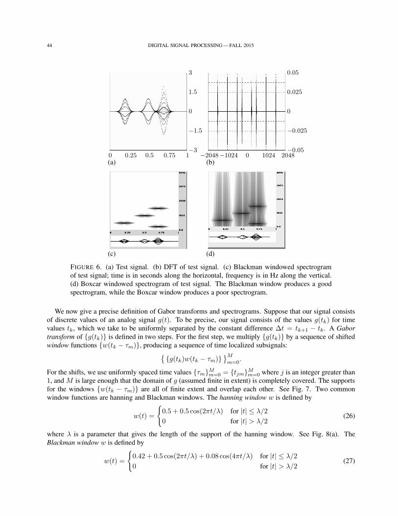
44 DIGITAL SIGNAL PROCESSING — FALL 2015
0 0.25 0.5 0.75 1−3
−1.5
0
1.5
3
(a)−2048−1024 0 1024 2048
−0.05
−0.025
0
0.025
0.05
(b)
(c) (d)
FIGURE 6. (a) Test signal. (b) DFT of test signal. (c) Blackman windowed spectrogram
of test signal; time is in seconds along the horizontal, frequency is in Hz along the vertical.
(d) Boxcar windowed spectrogram of test signal. The Blackman window produces a good
spectrogram, while the Boxcar window produces a poor spectrogram.
We now give a precise definition of Gabor transforms and spectrograms. Suppose that our signal consists
of discrete values of an analog signal g(t). To be precise, our signal consists of the values g(tk) for time
values tk, which we take to be uniformly separated by the constant difference ∆t = tk+1 − tk. A Gabor
transform of g(tk) is defined in two steps. For the first step, we multiply g(tk) by a sequence of shifted
window functions w(tk − τm), producing a sequence of time localized subsignals:g(tk)w(tk − τm)
Mm=0
.
For the shifts, we use uniformly spaced time values τmMm=0 = tjmMm=0 where j is an integer greater than
1, and M is large enough that the domain of g (assumed finite in extent) is completely covered. The supports
for the windows w(tk − τm) are all of finite extent and overlap each other. See Fig. 7. Two common
window functions are hanning and Blackman windows. The hanning window w is defined by
w(t) =
0.5 + 0.5 cos(2πt/λ) for |t| ≤ λ/2
0 for |t| > λ/2(26)
where λ is a parameter that gives the length of the support of the hanning window. See Fig. 8(a). The
Blackman window w is defined by
w(t) =
0.42 + 0.5 cos(2πt/λ) + 0.08 cos(4πt/λ) for |t| ≤ λ/2
0 for |t| > λ/2(27)
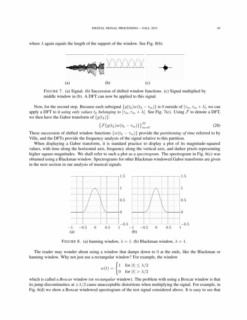
DIGITAL SIGNAL PROCESSING — FALL 2015 45
where λ again equals the length of the support of the window. See Fig. 8(b).
(a) (b) (c)
FIGURE 7. (a) Signal. (b) Succession of shifted window functions. (c) Signal multiplied by
middle window in (b). A DFT can now be applied to this signal.
Now, for the second step. Because each subsignal g(tk)w(tk − τm) is 0 outside of [τm, τm + λ], we can
apply a DFT to it using only values tk belonging to [τm, τm + λ]. See Fig. 7(c). Using F to denote a DFT,
we then have the Gabor transform of g(tk):Fg(tk)w(tk − τm)
Mm=0
. (28)
These succession of shifted window functions w(tk − τm) provide the partitioning of time referred to by
Ville, and the DFTs provide the frequency analysis of the signal relative to this partition.
When displaying a Gabor transform, it is standard practice to display a plot of its magnitude-squared
values, with time along the horizontal axis, frequency along the vertical axis, and darker pixels representing
higher square-magnitudes. We shall refer to such a plot as a spectrogram. The spectrogram in Fig. 6(c) was
obtained using a Blackman window. Spectrograms for other Blackman windowed Gabor transforms are given
in the next section in our analysis of musical signals.
−1 −0.5 0 0.5 1−0.5
0
0.5
1
1.5
(a)−1 −0.5 0 0.5 1
−0.5
0
0.5
1
1.5
(b)
FIGURE 8. (a) hanning window, λ = 1. (b) Blackman window, λ = 1.
The reader may wonder about using a window that damps down to 0 at the ends, like the Blackman or
hanning window. Why not just use a rectangular window? For example, the window
w(t) =
1 for |t| ≤ λ/2
0 for |t| > λ/2
which is called a Boxcar window (or rectangular window). The problem with using a Boxcar window is that
its jump discontinuities at ±λ/2 cause unacceptable distortions when multiplying the signal. For example, in
Fig. 6(d) we show a Boxcar windowed spectrogram of the test signal considered above. It is easy to see that
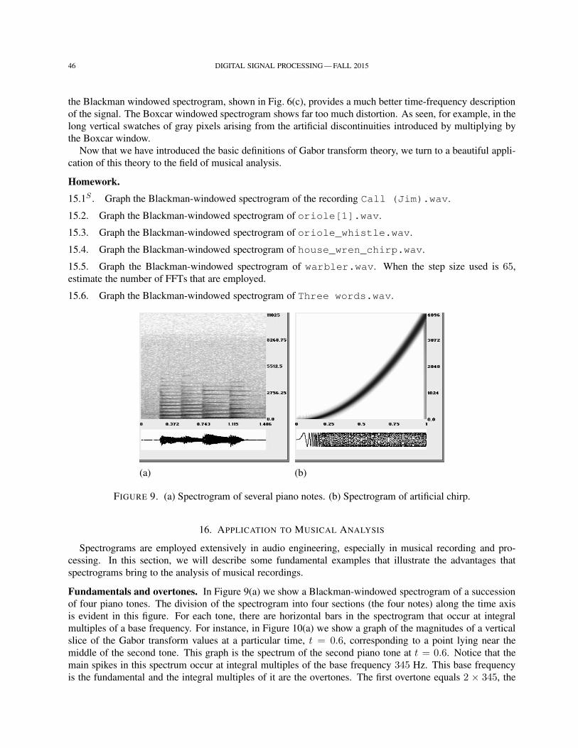
46 DIGITAL SIGNAL PROCESSING — FALL 2015
the Blackman windowed spectrogram, shown in Fig. 6(c), provides a much better time-frequency description
of the signal. The Boxcar windowed spectrogram shows far too much distortion. As seen, for example, in the
long vertical swatches of gray pixels arising from the artificial discontinuities introduced by multiplying by
the Boxcar window.
Now that we have introduced the basic definitions of Gabor transform theory, we turn to a beautiful appli-
cation of this theory to the field of musical analysis.
Homework.
15.1S . Graph the Blackman-windowed spectrogram of the recording Call (Jim).wav.
15.2. Graph the Blackman-windowed spectrogram of oriole[1].wav.
15.3. Graph the Blackman-windowed spectrogram of oriole_whistle.wav.
15.4. Graph the Blackman-windowed spectrogram of house_wren_chirp.wav.
15.5. Graph the Blackman-windowed spectrogram of warbler.wav. When the step size used is 65,
estimate the number of FFTs that are employed.
15.6. Graph the Blackman-windowed spectrogram of Three words.wav.
(a) (b)
FIGURE 9. (a) Spectrogram of several piano notes. (b) Spectrogram of artificial chirp.
16. APPLICATION TO MUSICAL ANALYSIS
Spectrograms are employed extensively in audio engineering, especially in musical recording and pro-
cessing. In this section, we will describe some fundamental examples that illustrate the advantages that
spectrograms bring to the analysis of musical recordings.
Fundamentals and overtones. In Figure 9(a) we show a Blackman-windowed spectrogram of a succession
of four piano tones. The division of the spectrogram into four sections (the four notes) along the time axis
is evident in this figure. For each tone, there are horizontal bars in the spectrogram that occur at integral
multiples of a base frequency. For instance, in Figure 10(a) we show a graph of the magnitudes of a vertical
slice of the Gabor transform values at a particular time, t = 0.6, corresponding to a point lying near the
middle of the second tone. This graph is the spectrum of the second piano tone at t = 0.6. Notice that the
main spikes in this spectrum occur at integral multiples of the base frequency 345 Hz. This base frequency
is the fundamental and the integral multiples of it are the overtones. The first overtone equals 2 × 345, the
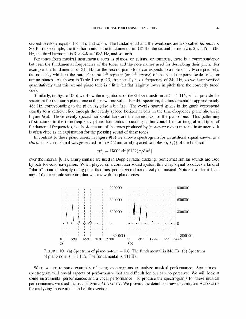
DIGITAL SIGNAL PROCESSING — FALL 2015 47
second overtone equals 3 × 345, and so on. The fundamental and the overtones are also called harmonics.
So, for this example, the first harmonic is the fundamental of 345 Hz, the second harmonic is 2× 345 = 690Hz, the third harmonic is 3× 345 = 1035 Hz, and so forth.
For tones from musical instruments, such as pianos, or guitars, or trumpets, there is a correspondence
between the fundamental frequencies of the tones and the note names used for describing their pitch. For
example, the fundamental of 345 Hz for the second piano tone corresponds to a note of F. More precisely,
the note F4, which is the note F in the 4th register (or 4th octave) of the equal-tempered scale used for
tuning pianos. As shown in Table 1 on p. 23, the note F4 has a frequency of 349 Hz, so we have verified
quantitatively that this second piano tone is a little bit flat (slightly lower in pitch than the correctly tuned
one).
Similarly, in Figure 10(b) we show the magnitudes of the Gabor transform at t = 1.115, which provide the
spectrum for the fourth piano tone at this new time value. For this spectrum, the fundamental is approximately
435 Hz, corresponding to the pitch A4 (also a bit flat). The evenly spaced spikes in the graph correspond
exactly to a vertical slice through the evenly spaced horizontal bars in the time-frequency plane shown in
Figure 9(a). Those evenly spaced horizontal bars are the harmonics for the piano tone. This patterning
of structures in the time-frequency plane, harmonics appearing as horizontal bars at integral multiples of
fundamental frequencies, is a basic feature of the tones produced by (non-percussive) musical instruments. It
is often cited as an explanation for the pleasing sound of these tones.
In contrast to these piano tones, in Figure 9(b) we show a spectrogram for an artificial signal known as a
chirp. This chirp signal was generated from 8192 uniformly spaced samples g(tk) of the function
g(t) = 15000 sin[8192(π/3)t3 ]
over the interval [0, 1). Chirp signals are used in Doppler radar tracking. Somewhat similar sounds are used
by bats for echo navigation. When played on a computer sound system this chirp signal produces a kind of
“alarm” sound of sharply rising pitch that most people would not classify as musical. Notice also that it lacks
any of the harmonic structure that we saw with the piano tones.
0 690 1380 2070 2760−300000
0
300000
600000
900000
(a)0 862 1724 2586 3448
−300000
0
300000
600000
900000
(b)
FIGURE 10. (a) Spectrum of piano note, t = 0.6. The fundamental is 345 Hz. (b) Spectrum
of piano note, t = 1.115. The fundamental is 431 Hz.
We now turn to some examples of using spectrograms to analyze musical performance. Sometimes a
spectrogram will reveal aspects of performance that are difficult for our ears to perceive. We will look at
some instrumental performances and a vocal performance. To produce the spectrograms for these musical
performances, we used the free software AUDACITY. We provide the details on how to configure AUDACITY
for analyzing music at the end of this section.
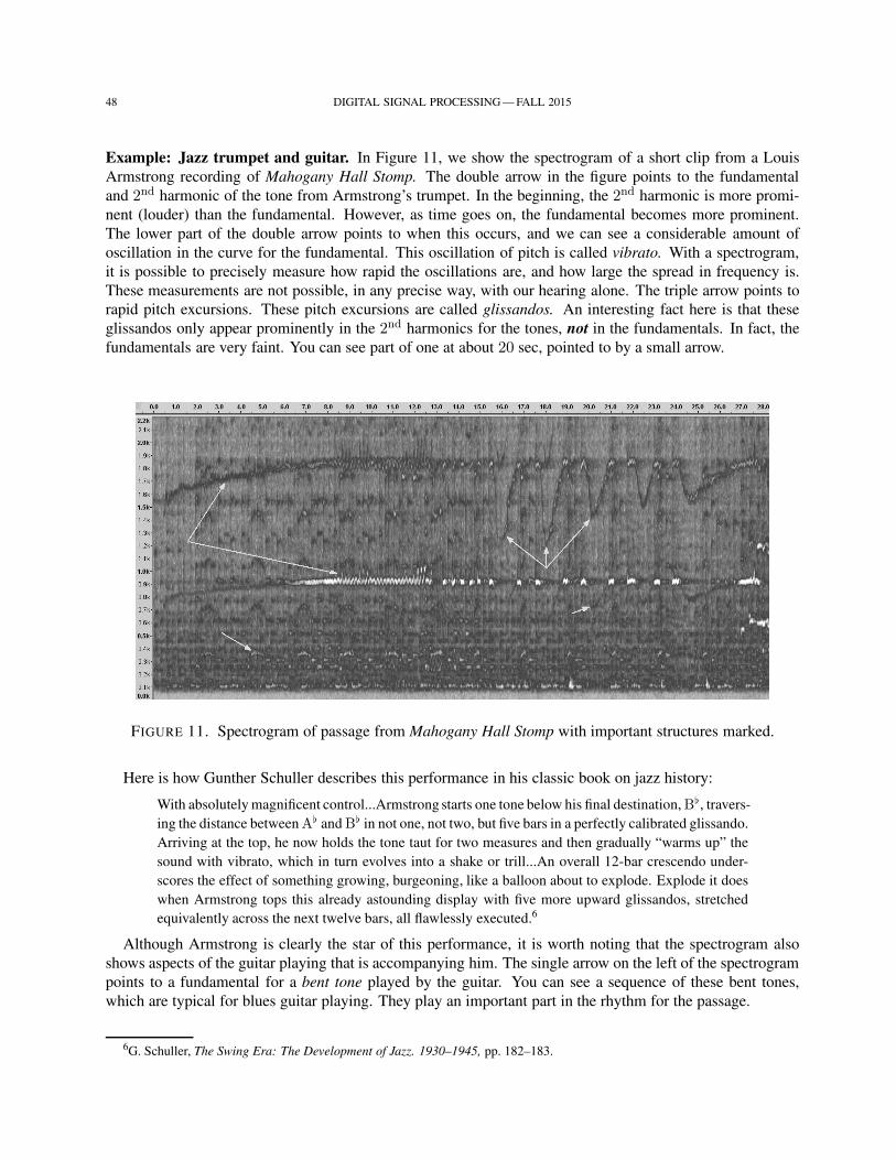
48 DIGITAL SIGNAL PROCESSING — FALL 2015
Example: Jazz trumpet and guitar. In Figure 11, we show the spectrogram of a short clip from a Louis
Armstrong recording of Mahogany Hall Stomp. The double arrow in the figure points to the fundamental
and 2nd harmonic of the tone from Armstrong’s trumpet. In the beginning, the 2nd harmonic is more promi-
nent (louder) than the fundamental. However, as time goes on, the fundamental becomes more prominent.
The lower part of the double arrow points to when this occurs, and we can see a considerable amount of
oscillation in the curve for the fundamental. This oscillation of pitch is called vibrato. With a spectrogram,
it is possible to precisely measure how rapid the oscillations are, and how large the spread in frequency is.
These measurements are not possible, in any precise way, with our hearing alone. The triple arrow points to
rapid pitch excursions. These pitch excursions are called glissandos. An interesting fact here is that these
glissandos only appear prominently in the 2nd harmonics for the tones, not in the fundamentals. In fact, the
fundamentals are very faint. You can see part of one at about 20 sec, pointed to by a small arrow.
FIGURE 11. Spectrogram of passage from Mahogany Hall Stomp with important structures marked.
Here is how Gunther Schuller describes this performance in his classic book on jazz history:
With absolutely magnificent control...Armstrong starts one tone below his final destination,B, travers-
ing the distance betweenA and B in not one, not two, but five bars in a perfectly calibrated glissando.
Arriving at the top, he now holds the tone taut for two measures and then gradually “warms up” the
sound with vibrato, which in turn evolves into a shake or trill...An overall 12-bar crescendo under-
scores the effect of something growing, burgeoning, like a balloon about to explode. Explode it does
when Armstrong tops this already astounding display with five more upward glissandos, stretched
equivalently across the next twelve bars, all flawlessly executed.6
Although Armstrong is clearly the star of this performance, it is worth noting that the spectrogram also
shows aspects of the guitar playing that is accompanying him. The single arrow on the left of the spectrogram
points to a fundamental for a bent tone played by the guitar. You can see a sequence of these bent tones,
which are typical for blues guitar playing. They play an important part in the rhythm for the passage.
6G. Schuller, The Swing Era: The Development of Jazz. 1930–1945, pp. 182–183.
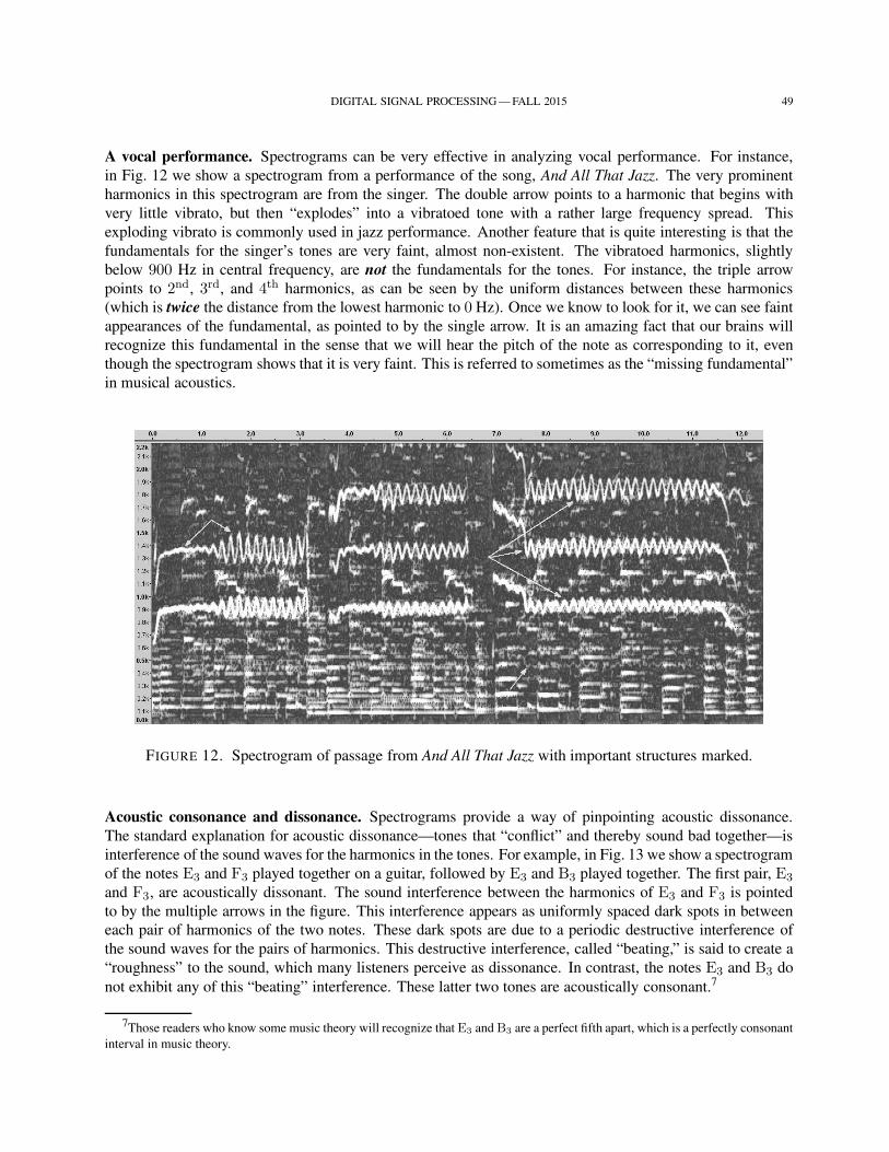
DIGITAL SIGNAL PROCESSING — FALL 2015 49
A vocal performance. Spectrograms can be very effective in analyzing vocal performance. For instance,
in Fig. 12 we show a spectrogram from a performance of the song, And All That Jazz. The very prominent
harmonics in this spectrogram are from the singer. The double arrow points to a harmonic that begins with
very little vibrato, but then “explodes” into a vibratoed tone with a rather large frequency spread. This
exploding vibrato is commonly used in jazz performance. Another feature that is quite interesting is that the
fundamentals for the singer’s tones are very faint, almost non-existent. The vibratoed harmonics, slightly
below 900 Hz in central frequency, are not the fundamentals for the tones. For instance, the triple arrow
points to 2nd, 3rd, and 4th harmonics, as can be seen by the uniform distances between these harmonics
(which is twice the distance from the lowest harmonic to 0 Hz). Once we know to look for it, we can see faint
appearances of the fundamental, as pointed to by the single arrow. It is an amazing fact that our brains will
recognize this fundamental in the sense that we will hear the pitch of the note as corresponding to it, even
though the spectrogram shows that it is very faint. This is referred to sometimes as the “missing fundamental”
in musical acoustics.
FIGURE 12. Spectrogram of passage from And All That Jazz with important structures marked.
Acoustic consonance and dissonance. Spectrograms provide a way of pinpointing acoustic dissonance.
The standard explanation for acoustic dissonance—tones that “conflict” and thereby sound bad together—is
interference of the sound waves for the harmonics in the tones. For example, in Fig. 13 we show a spectrogram
of the notes E3 and F3 played together on a guitar, followed by E3 and B3 played together. The first pair, E3
and F3, are acoustically dissonant. The sound interference between the harmonics of E3 and F3 is pointed
to by the multiple arrows in the figure. This interference appears as uniformly spaced dark spots in between
each pair of harmonics of the two notes. These dark spots are due to a periodic destructive interference of
the sound waves for the pairs of harmonics. This destructive interference, called “beating,” is said to create a
“roughness” to the sound, which many listeners perceive as dissonance. In contrast, the notes E3 and B3 do
not exhibit any of this “beating” interference. These latter two tones are acoustically consonant.7
7Those readers who know some music theory will recognize that E3 and B3 are a perfect fifth apart, which is a perfectly consonant
interval in music theory.
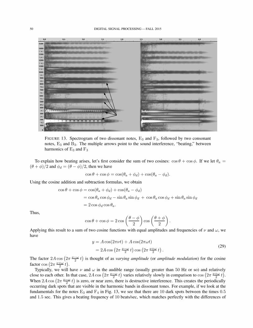
50 DIGITAL SIGNAL PROCESSING — FALL 2015
FIGURE 13. Spectrogram of two dissonant notes, E3 and F3, followed by two consonant
notes, E3 and B3. The multiple arrows point to the sound interference, “beating,” between
harmonics of E3 and F3
To explain how beating arises, let’s first consider the sum of two cosines: cos θ + cosφ. If we let θa =(θ + φ)/2 and φd = (θ − φ)/2, then we have
cos θ + cosφ = cos(θa + φd) + cos(θa − φd).
Using the cosine addition and subtraction formulas, we obtain
cos θ + cosφ = cos(θa + φd) + cos(θa − φd)
= cos θa cosφd − sin θa sinφd + cos θa cosφd + sin θa sinφd
= 2cos φd cos θa.
Thus,
cos θ + cosφ = 2cos
(θ − φ
2
)cos
(θ + φ
2
).
Applying this result to a sum of two cosine functions with equal amplitudes and frequencies of ν and ω, we
have
y = A cos(2πνt) +A cos(2πωt)
= 2A cos(2π ν−ω
2 t)cos(2π ν+ω
2 t).
(29)
The factor 2A cos(2π ν−ω
2 t)
is thought of as varying amplitude (or amplitude modulation) for the cosine
factor cos(2π ν+ω
2 t).
Typically, we will have ν and ω in the audible range (usually greater than 50 Hz or so) and relatively
close to each other. In that case, 2A cos(2π ν−ω
2 t)
varies relatively slowly in comparison to cos(2π ν+ω
2 t).
When 2A cos(2π ν−ω
2 t)
is zero, or near zero, there is destructive interference. This creates the periodically
occurring dark spots that are visible in the harmonic bands in dissonant tones. For example, if we look at the
fundamentals for the notes E3 and F4 in Fig. 13, we see that there are 10 dark spots between the times 0.5and 1.5 sec. This gives a beating frequency of 10 beats/sec, which matches perfectly with the differences of
DIGITAL SIGNAL PROCESSING — FALL 2015 51
the fundamental frequencies: 175 − 165 = 10. We leave at as an exercise for the reader to check that the
beating frequencies for the second and third harmonics of E3 and F4 also match the difference in frequencies
between these harmonics for the two notes.
Acoustic dissonance occurs frequently in music. As an example, we show in Fig. 15, a spectrogram from
the beginning of a recording of Layla. There is acoustic dissonance in a number of places between different
guitar harmonics.
Additional Musical Analyses. We have only scratched the surface of how spectrograms aid in the analysis
of musical performance. Many more examples are described in the book:
J.S. Walker and G.W. Don, Mathematics and Music: Composition, Perception, and Performance, CRC Press, 2013.
That book is used a reference for the course
MATH 307: Mathematics and Music, http://people.uwec.edu/walkerjs/MandM/
which is offered online in the summer.
Using AUDACITY for music files. The installation program for AUDACITY can be found here:
http://audacity.sourceforge.net/download/
The software is free to download, and runs on most computers.
To configure AUDACITY for analyzing music, select the Edit menu and choose Preferences. (On a MAC,
you select Preferences from the Audacity menu.) From the list of choices shown on the left of the preferences
window, select Spectrograms. Then make the following three changes:
(1) Change the FFT size, which is listed as 256, to 4096.
(2) Change the Window type, which is listed as Hanning, to Blackman.
(3) Change the Maximum frequency, which is listed as 8000, to 3000.
After making these changes, click the OK button. AUDACITY is now configured for analyzing music. It will
remember these settings in the future, so you won’t have to change them again. The only exception is the
setting for the Maximum frequency value, which you might want to change for different types of music.
To load a music file, select the File menu and choose Open. (Or, you can also choose Import and then
Audio.) AUDACITY recognizes most common formats for music files, such as .wav and .mp3 files. When
you load a music file, you will see a blue-colored graph displayed on the screen. It is a graph of the electrical
current oscillations in the recording of the music, the music’s waveform. To display a spectrogram, you do
the following. Click on a small box on the left of the screen, adjacent to the graph displayed, containing the
name of the music file. (See Figure 14.) A menu will appear, and you select Spectrogram from this menu.
(Do not select Spectrogram log(f), we will not be using that option.) After you have selected Spectrogram,
AUDACITY will display a spectrogram of the music.
To get a good view of the spectrogram, it is best to grab the lower border of its graph and pull it down to
expand the view. Also, if the music you selected is a stereo recording, then two spectrograms are displayed.
Often it is best to just have one spectrogram. To plot just one spectrogram for stereo music, select the Tracks
menu and choose Stereo to mono.
Homework.
16.1. In the quotation from Gunther Schuller, he says that Armstrong’s long glissando goes from A to B.
Are those notes correct, based on Table 1 on p. 23 and the spectrogram in Fig. 11?
16.2S . In our description of Mahogany Hall Stomp, we referred to some bent guitar tones. What note are
those tones approximate to?
16.3. In the spectrogram for And All That Jazz, in Fig. 12, the singer is singing the same note on all three
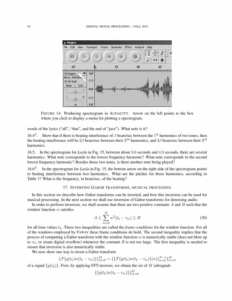
52 DIGITAL SIGNAL PROCESSING — FALL 2015
FIGURE 14. Producing spectrogram in AUDACITY. Arrow on the left points to the box
where you click to display a menu for plotting a spectrogram.
words of the lyrics (“all”, “that”, and the end of “jazz”). What note is it?
16.4S . Show that if there is beating interference of β beats/sec between the 1st harmonics of two tones, then
the beating interference will be 2β beats/sec between their 2nd harmonics, and 3β beats/sec between their 3rd
harmonics.
16.5. In the spectrogram for Layla in Fig. 15, between about 3.6 seconds and 4.0 seconds, there are several
harmonics. What note corresponds to the lowest frequency harmonic? What note corresponds to the second
lowest frequency harmonic? Besides those two notes, is there another note being played?
16.6S . In the spectrogram for Layla in Fig. 15, the bottom arrow on the right side of the spectrogram points
to beating interference between two harmonics. What are the pitches for those harmonics, according to
Table 1? What is the frequency, in beats/sec, of the beating?
17. INVERTING GABOR TRANSFORMS, MUSICAL PROCESSING
In this section we describe how Gabor transforms can be inverted, and how this inversion can be used for
musical processing. In the next section we shall use inversion of Gabor transforms for denoising audio.
In order to perform inversion, we shall assume that there are two positive constants A and B such that the
window function w satisfies
A ≤M∑
m=0
w2(tk − τm) ≤ B (30)
for all time values tk. These two inequalities are called the frame conditions for the window function. For all
of the windows employed by FAWAV these frame conditions do hold. The second inequality implies that the
process of computing a Gabor transform with the window function w is numerically stable (does not blow up
to ∞, or create digital overflow) whenever the constant B is not too large. The first inequality is needed to
ensure that inversion is also numerically stable.
We now show one way to invert a Gabor transform
Fg(tk)w(tk − τm)Mm=0 = Fg(tk)w(tk − τm)(n)N−1n=0 Mm=0
of a signal g(tk). First, by applying FFT-inverses, we obtain the set of M subsignals
g(tk)w(tk − τm)Mm=0.
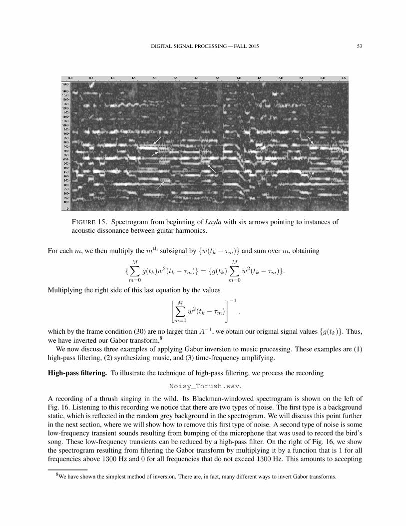
DIGITAL SIGNAL PROCESSING — FALL 2015 53
FIGURE 15. Spectrogram from beginning of Layla with six arrows pointing to instances of
acoustic dissonance between guitar harmonics.
For each m, we then multiply the mth subsignal by w(tk − τm) and sum over m, obtaining
M∑
m=0
g(tk)w2(tk − τm) = g(tk)
M∑
m=0
w2(tk − τm).
Multiplying the right side of this last equation by the values
[M∑
m=0
w2(tk − τm)
]−1
,
which by the frame condition (30) are no larger than A−1, we obtain our original signal values g(tk). Thus,
we have inverted our Gabor transform.8
We now discuss three examples of applying Gabor inversion to music processing. These examples are (1)
high-pass filtering, (2) synthesizing music, and (3) time-frequency amplifying.
High-pass filtering. To illustrate the technique of high-pass filtering, we process the recording
Noisy_Thrush.wav.
A recording of a thrush singing in the wild. Its Blackman-windowed spectrogram is shown on the left of
Fig. 16. Listening to this recording we notice that there are two types of noise. The first type is a background
static, which is reflected in the random grey background in the spectrogram. We will discuss this point further
in the next section, where we will show how to remove this first type of noise. A second type of noise is some
low-frequency transient sounds resulting from bumping of the microphone that was used to record the bird’s
song. These low-frequency transients can be reduced by a high-pass filter. On the right of Fig. 16, we show
the spectrogram resulting from filtering the Gabor transform by multiplying it by a function that is 1 for all
frequencies above 1300 Hz and 0 for all frequencies that do not exceed 1300 Hz. This amounts to accepting
8We have shown the simplest method of inversion. There are, in fact, many different ways to invert Gabor transforms.
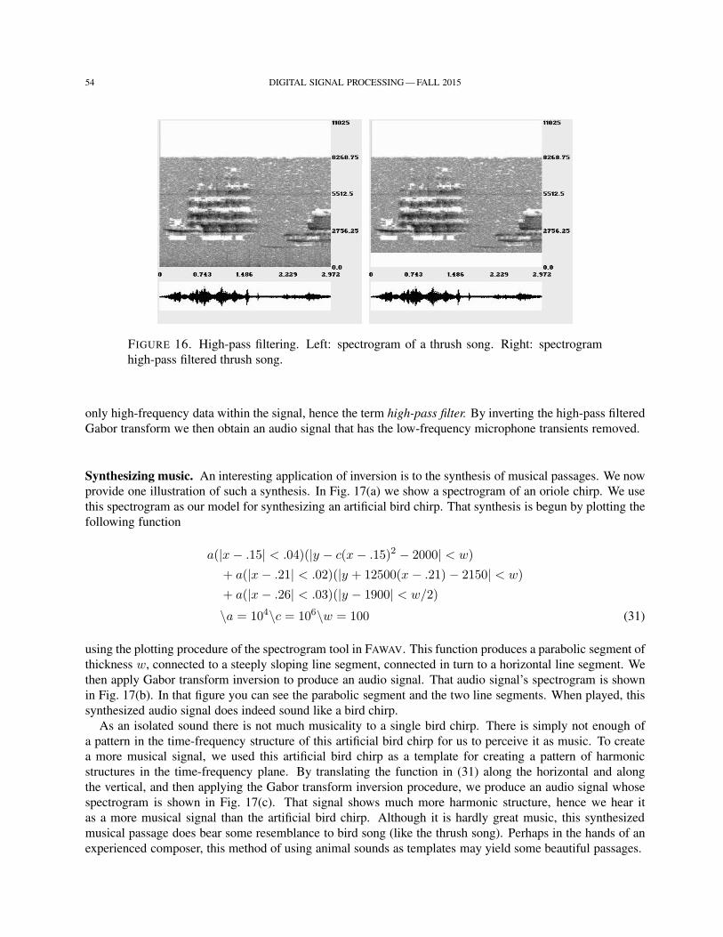
54 DIGITAL SIGNAL PROCESSING — FALL 2015
FIGURE 16. High-pass filtering. Left: spectrogram of a thrush song. Right: spectrogram
high-pass filtered thrush song.
only high-frequency data within the signal, hence the term high-pass filter. By inverting the high-pass filtered
Gabor transform we then obtain an audio signal that has the low-frequency microphone transients removed.
Synthesizing music. An interesting application of inversion is to the synthesis of musical passages. We now
provide one illustration of such a synthesis. In Fig. 17(a) we show a spectrogram of an oriole chirp. We use
this spectrogram as our model for synthesizing an artificial bird chirp. That synthesis is begun by plotting the
following function
a(|x− .15| < .04)(|y − c(x− .15)2 − 2000| < w)
+ a(|x− .21| < .02)(|y + 12500(x − .21) − 2150| < w)
+ a(|x− .26| < .03)(|y − 1900| < w/2)
\a = 104\c = 106\w = 100 (31)
using the plotting procedure of the spectrogram tool in FAWAV. This function produces a parabolic segment of
thickness w, connected to a steeply sloping line segment, connected in turn to a horizontal line segment. We
then apply Gabor transform inversion to produce an audio signal. That audio signal’s spectrogram is shown
in Fig. 17(b). In that figure you can see the parabolic segment and the two line segments. When played, this
synthesized audio signal does indeed sound like a bird chirp.
As an isolated sound there is not much musicality to a single bird chirp. There is simply not enough of
a pattern in the time-frequency structure of this artificial bird chirp for us to perceive it as music. To create
a more musical signal, we used this artificial bird chirp as a template for creating a pattern of harmonic
structures in the time-frequency plane. By translating the function in (31) along the horizontal and along
the vertical, and then applying the Gabor transform inversion procedure, we produce an audio signal whose
spectrogram is shown in Fig. 17(c). That signal shows much more harmonic structure, hence we hear it
as a more musical signal than the artificial bird chirp. Although it is hardly great music, this synthesized
musical passage does bear some resemblance to bird song (like the thrush song). Perhaps in the hands of an
experienced composer, this method of using animal sounds as templates may yield some beautiful passages.
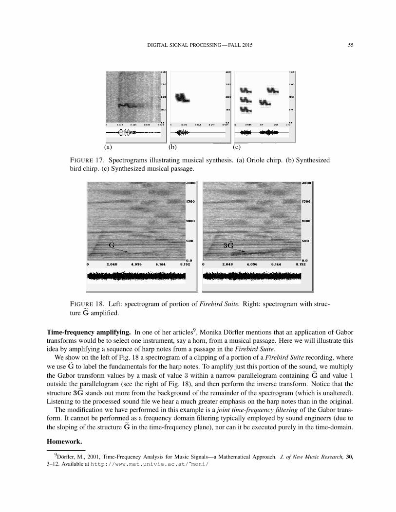
DIGITAL SIGNAL PROCESSING — FALL 2015 55
(a) (b) (c)
FIGURE 17. Spectrograms illustrating musical synthesis. (a) Oriole chirp. (b) Synthesized
bird chirp. (c) Synthesized musical passage.
GXXXz
3GXXXz
FIGURE 18. Left: spectrogram of portion of Firebird Suite. Right: spectrogram with struc-
ture G amplified.
Time-frequency amplifying. In one of her articles9, Monika Dorfler mentions that an application of Gabor
transforms would be to select one instrument, say a horn, from a musical passage. Here we will illustrate this
idea by amplifying a sequence of harp notes from a passage in the Firebird Suite.
We show on the left of Fig. 18 a spectrogram of a clipping of a portion of a Firebird Suite recording, where
we use G to label the fundamentals for the harp notes. To amplify just this portion of the sound, we multiply
the Gabor transform values by a mask of value 3 within a narrow parallelogram containing G and value 1outside the parallelogram (see the right of Fig. 18), and then perform the inverse transform. Notice that the
structure 3G stands out more from the background of the remainder of the spectrogram (which is unaltered).
Listening to the processed sound file we hear a much greater emphasis on the harp notes than in the original.
The modification we have performed in this example is a joint time-frequency filtering of the Gabor trans-
form. It cannot be performed as a frequency domain filtering typically employed by sound engineers (due to
the sloping of the structure G in the time-frequency plane), nor can it be executed purely in the time-domain.
Homework.
9Dorfler, M., 2001, Time-Frequency Analysis for Music Signals—a Mathematical Approach. J. of New Music Research, 30,
3–12. Available at http://www.mat.univie.ac.at/~moni/
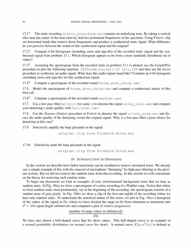
56 DIGITAL SIGNAL PROCESSING — FALL 2015
17.1S . The static recording static_recording.wav contains an underlying tone. By taking a vertical
slice near the center of the time interval, find two prominent frequencies in the spectrum. Using FAWAV, clip
out horizontal bands that remove those frequencies and produce a synthesized static signal. What difference
do you perceive between the sound of this synthesized signal and the original?
17.2S . Compute 8-bit histograms (including zeros and sign-bit) of the recorded static signal and the syn-
thesized signal from problem 17.1. Which histogram appears to be from a more randomly distributed set of
values?
17.3S . Assuming the spectrogram from the recorded static in problem 17.1 is plotted, use the Graph/Plot
procedure to plot the following function: 2000sumk(ran(x))/10 \k=1,100 and then use the Invert
procedure to synthesize an audio signal. What does this audio signal sound like? Compute an 8-bit histogram
(including zeros and sign-bit) for this synthesized signal.
17.4S . Compute a spectrogram of the recorded sound house_wren_chirp.wav.
17.5. Model the spectrogram of house_wren_chirp.wav and compute a synthesized mimic of this
bird call.
17.6S . Compute a spectrogram of the recorded sound warbler.wav.
17.7. Use a low-pass filter (g1(y<c) for some c) to denoise the signal noisy_call.wav and compare
your denoising’s audio quality with Call(Jim).wav.
17.8. Use the Denoise (Gabor) procedure in FAWAV to denoise the signal oriole_song.wav and dis-
cuss the audio quality of the denoising versus the original signal. Why is a low-pass filter a poor choice for
denoising in this case?
17.9. Selectively amplify the harp glissando in the signal:
original clip from Firebird Suite.wav.
17.10. Selectively mute the harp glissando in the signal:
original clip from Firebird Suite.wav.
18. INTRODUCTION TO DENOISING
In this section we describe how Gabor transforms can be modified to remove unwanted noise. We already
saw a simple example of this with the removal of microphone “thumping” by high-pass filtering in the previ-
ous section. But we did not remove the random static from that recording. In this section we will concentrate
on the theory for removing such random static.
To begin our discussion we look at examples of real, environmental background noise that we hear as
random static. In Fig. 19(a) we show a spectrogram of a noisy recording of a Warbler song. Notice that where
we hear random static most prominently, say at the beginning of the recording, the spectrogram consists of a
random array of grey pixels. In Fig. 19(b) we show a clip of the first one-eighth of the recording where we
hear only random static. To understand the statistical nature of this noise, we plot in Fig. 19(c) a histogram
of the values of the signal in (b), where we have divided the range in (b) from minimum to maximum into
28 = 256 equal-length subintervals and computed a plot of relative frequencies:
(number of range values in subinterval)
256.
We have also drawn a bell-shaped curve that fits those values. This bell-shaped curve is an example of
a normal probability distribution (or normal curve for short). A normal curve N (µ, σ2)(x) is defined as
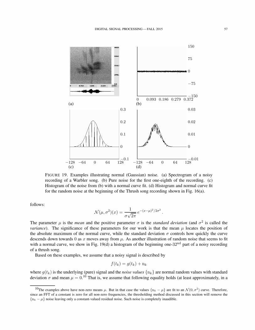
DIGITAL SIGNAL PROCESSING — FALL 2015 57
(a)0 0.093 0.186 0.279 0.372
−150
−75
0
75
150
(b)
−128 −64 0 64 128−0.1
0
0.1
0.2
0.3
(c)−128 −64 0 64 128
−0.01
0
0.01
0.02
0.03
(d)
FIGURE 19. Examples illustrating normal (Gaussian) noise. (a) Spectrogram of a noisy
recording of a Warbler song. (b) Pure noise for the first one-eighth of the recording. (c)
Histogram of the noise from (b) with a normal curve fit. (d) Histogram and normal curve fit
for the random noise at the beginning of the Thrush song recording shown in Fig. 16(a).
follows:
N (µ, σ2)(x) =1
σ√2π
e−(x−µ)2/2σ2.
The parameter µ is the mean and the positive parameter σ is the standard deviation (and σ2 is called the
variance). The significance of these parameters for our work is that the mean µ locates the position of
the absolute maximum of the normal curve, while the standard deviation σ controls how quickly the curve
descends down towards 0 as x moves away from µ. As another illustration of random noise that seems to fit
with a normal curve, we show in Fig. 19(d) a histogram of the beginning one-32nd part of a noisy recording
of a thrush song.
Based on these examples, we assume that a noisy signal is described by
f(tk) = g(tk) + nk
where g(tk) is the underlying (pure) signal and the noise values nk are normal random values with standard
deviation σ and mean µ = 0.10 That is, we assume that following equality holds (at least approximately, in a
10The examples above have non-zero means µ. But in that case the values nk − µ are fit to an N (0, σ2) curve. Therefore,
since an FFT of a constant is zero for all non-zero frequencies, the thresholding method discussed in this section will remove the
nk − µ noise leaving only a constant-valued residual noise. Such noise is completely inaudible.
58 DIGITAL SIGNAL PROCESSING — FALL 2015
statistical sense):
(Fraction of values nk lying between α and β) =
∫ β
α
1
σ√2π
e−x2/2σ2dx. (32)
where α < β are any two possible real numbers. Equality (32) follows from the law of large numbers
discussed in an introductory course in either Statistics or Mathematical Probability. Equality (32) uses the
standard deviation σ. One way to estimate σ is to isolate a portion of the signal consisting purely of noise11
and use a basic statistical formula to estimate σ. FAWAV does this using its Analysis/Statistics procedure.
We now prove the following theorem, which provides a universal threshold for Gaussian noise.
Theorem 1. For Gaussian normal noise of mean 0 and standard deviation σ, the probability that the magni-
tude of a value is larger than To = σ√2 logN is significantly less than 1/N for sufficiently large N (by a
factor that tends to 0 as N → ∞).
Proof. Because the noise values are Gaussian normal [i.e. of type N (0, σ2)], it follows that for any positive
a we have
Prob(|noise value| > aσ) = 1− Prob(|noise value| ≤ aσ)
=
∫ ∞
−∞
1
σ√2π
e−x2/2σ2dx−
∫ aσ
−aσ
1
σ√2π
e−x2/2σ2dx
=
∫ −aσ
−∞
1
σ√2π
e−x2/2σ2dx+
∫ ∞
aσ
1
σ√2π
e−x2/2σ2dx
=
∫ ∞
aσ
2
σ√2π
e−x2/2σ2dx.
The last integral is simplified by a change of variables (x = σt, dx = σ dt):∫ ∞
aσ
2
σ√2π
e−x2/2σ2dx =
∫ ∞
a
2√2π
e−t2/2 dt.
We bound this last integral as follows:∫ ∞
a
2√2π
e−t2/2 dt ≤∫ ∞
a
2√2π
t
ae−t2/2 dt (because 1 ≤ t
afor t ≥ a)
=−2
a√2π
e−t2/2
∣∣∣∣t→∞
t=a
=2
a√2π
e−a2/2.
Putting a =√2 logN in the last expression, we obtain
2
a√2π
e−a2/2 =1√
π logN
1
N.
Therefore, we have
Prob(|noise value| > σ√
2 logN) ≤ 1√π logN
1
N.
Since 1/√π logN → 0 as N → ∞, we can see that the factor multiplying 1/N does tend to 0. Furthermore,
for N ≥ 256 we get 1/√π logN ≤ 0.25. Hence, the bound on the right is significantly less than 1/N , for
N ≥ 256. Thus, our result is proved.
11Of course that can’t always be done; we discuss that issue later on.
DIGITAL SIGNAL PROCESSING — FALL 2015 59
From this theorem, we conclude that the fraction of magnitudes of nk lying within each window whose
magnitude is below To is (almost surely) 100%. Therefore, by thresholding the noisy signal: setting to 0 all
values that have magnitude less than To; we will be certain to remove isolated noise values. Unfortunately,
there is a big problem with such a naive approach. Because noise values are added to signal values, they are
generally not isolated and, therefore, will not be removed by this thresholding.
The way around the problem is to perform a Gabor transform of the noisy signal values. Because f = g+n,
a Gabor transform of f(tk) satisfies
Ff(tk)w(tk − τm)Mm=0 = Fg(tk)w(tk − τm)Mm=0 + Fnkw(tk − τm)Mm=0. (33)
This last equation can be rewritten as
Ff(tk)w(tk − τm)tk∈ImMm=0 = Fg(tk)w(tk − τm)tk∈ImMm=0 + Fnkw(tk − τm)tk∈ImMm=0
where Im is the set of values tk satisfying |tk − τm| ≤ λ/2. We shall now discuss why we may expect
that 100% of the values of the noise’s Gabor transform, Fnkw(tk − τm)tk∈ImMm=0, will be smaller in
magnitude than a constant multiple of σ√2 logN .
To begin our discussion, we briefly review the definition of expectation, and its relation to Gaussian random
noise. The expectation of the random variable y = h(x), where x is a random variable, is denoted E(h) and
defined as
E(h)= lim
K→∞1
K
K∑
k=1
yk (34)
where N measurements yk of y are taken. Here are some basic facts about expectation, and its relation to
Gaussian random noise:
(1) LINEARITY. For functions h1(x) and h2(x), and constants c1 and c2, we have
E(c1h1 + c2h2
)= c1E
(h1)+ c2E
(h2).
(2) For any constant c, we have E(c)= c.
(3) If xi and xj are independent random variables, then E(xixj
)= 0.
(4) When x is of type N (0, σ2), then the Law of Large Numbers implies that the expectation for h(x)satisfies
E(h)=
1√2π σ
∫ ∞
−∞h(x) e−x2/2σ2
dx.
In particular, we have E(c) =1√2π σ
∫ ∞
−∞c e−x2/2σ2
dx = c, which is consistent with property (2).
(5) For each noise value nk, we have
E(nk)= 0
=1√2π σ
∫ ∞
−∞x e−x2/2σ2
dx
and
E(n2k)= σ2
=1√2π σ
∫ ∞
−∞x2 e−x2/2σ2
dx.
In addition to these basic facts about expectation, we also need the following two linearity properties of
Gaussian normal random variables:
60 DIGITAL SIGNAL PROCESSING — FALL 2015
(A) If x is a random variable of type N (0, σ2) and a is a real constant, then ax is a random variable of
type N (0, a2σ2). [Note: if a = 0, then ax = 0 and that is consistent with type N (0, 0).]
(B) If x1 and x2 are independent random variables of type N (0, σ21) and N (0, σ2
2), respectively, then
x1+x2 is a random variable of type N (0, σ21 +σ2
2). [Notice that this says that the variance of x1+x2is the sum of the variances of x1 and x2.]
We will not prove these elementary properties, which are discussed in pretty much every introductory statistics
book, e.g., the text A Modern Introduction to Probability and Statistics: Understanding Why and How
by F.M. Dekking, et. al., has a nice treatment. It is important to note that properties (A) and (B) can be
combined repeatedly to prove the following theorem.
Theorem 2. If xkKk=0 is a finite set of mutually independent random variables, each xk of type N (0, σ2k),
then every linear combination,
K∑
k=0
akxk, for real constants ak, is type N (0, σ2). Moreover, σ2 =K∑
k=0
a2kσ2k.
We have now discussed all of the ideas that we need to prove a bound on the values of the Gabor transform
of the noise. To be precise, we have the following theorem.
Theorem 3. Almost surely 100% of the Gabor noise transform values, Fnkw(tk − τm)tk∈ImMm=0, are
smaller in magnitude than c σ√2 logN , where c
.= 0.552
√N .
Proof. For each windowing, we are dealing with noise values nkN−1k=0 arising from specific values taken
from a collection of real-valued random variables xkN−1k=0 . We assume that these random variables xkN−1
k=0
are mutually independent, and that each one is type N (0, σ2). Now, fix a value of m. We will show that the
required bound holds for the values Fxkw(tk − τm)tk∈Im. Since m is an arbitrary choice from the set
0, 1, . . . ,M, this will be sufficient for proving the theorem.
To simplify notation, let bk = w(tk − τm) for each k. Then, we need to bound Fbkxktk∈Im. By the
definition of F we have Xn = Fbkxk, i.e., for each n,
Xn =
N−1∑
k=0
bkxke−i2πkn/N .
where, as a further notational simplification, we are assuming that the index k begins at 0 for tk ∈ Im.
DIGITAL SIGNAL PROCESSING — FALL 2015 61
Computing E(|Xn|2
)is done as follows:
E(|Xn|2
)= E
(
N−1∑
k=0
bkxke−i2πkn/N
)
N−1∑
j=0
bjxje−i2πjn/N
= E
(
N−1∑
k=0
bkxke−i2πkn/N
)
N−1∑
j=0
bjxje+i2πjn/N
= E
N−1∑
k=0
N−1∑
j=0
bkbjei2π(j−k)n/Nxjxk
=
N−1∑
k=0
N−1∑
j=0
bkbjei2π(j−k)n/N
E(xjxk
)
=N−1∑
k=0
N−1∑
j=0
bkbjei2π(j−k)n/Nδj,k σ
2
where δj,k = 0 if k 6= j and δj,k = 1 if k = j. Using this definition of δj,k the last line above simplifies, and
we obtain
E(|Xn|2
)=
N−1∑
k=0
b2k σ2
= c2σ2
(35)
where the constant c is defined by
c =
√√√√N−1∑
k=0
b2k . (36)
Later in the proof, we will show that c.= 0.552
√N . But, before we do that, we will show how (35) leads
to the desired bound for the values of the Gabor transform of the noise. We define the transforms Cn and
Sn as follows:
Cn =
N−1∑
k=0
bkxk cos(2πkn/N) and Sn =
N−1∑
k=0
bkxk sin(2πkn/N).
Because of Euler’s identity, e−iθ = cos θ − i sin θ, we have
Xn = Cn − iSn.
Moreover, by Theorem 2, each Cn and Sn is a normal random variable. We denote the variance of Cn by σ2n
and the variance of Sn by σ2n. Because Xn = Cn − iSn, we have
|Xn|2 = C2n + S2
n
and, because E(C2n
)= σ2
n and E(S2n
)= σ2
n, we then have
E(|Xn|2
)= E
(C2n + S2
n
)
= E(C2n
)+E(S2n
)
= σ2n + σ2
n.
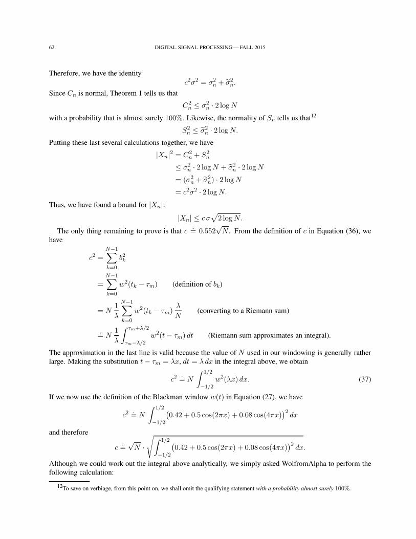
62 DIGITAL SIGNAL PROCESSING — FALL 2015
Therefore, we have the identity
c2σ2 = σ2n + σ2
n.
Since Cn is normal, Theorem 1 tells us that
C2n ≤ σ2
n · 2 logNwith a probability that is almost surely 100%. Likewise, the normality of Sn tells us that12
S2n ≤ σ2
n · 2 logN.
Putting these last several calculations together, we have
|Xn|2 = C2n + S2
n
≤ σ2n · 2 logN + σ2
n · 2 logN= (σ2
n + σ2n) · 2 logN
= c2σ2 · 2 logN.
Thus, we have found a bound for |Xn|:|Xn| ≤ c σ
√2 logN.
The only thing remaining to prove is that c.= 0.552
√N . From the definition of c in Equation (36), we
have
c2 =N−1∑
k=0
b2k
=N−1∑
k=0
w2(tk − τm) (definition of bk)
= N1
λ
N−1∑
k=0
w2(tk − τm)λ
N(converting to a Riemann sum)
.= N
1
λ
∫ τm+λ/2
τm−λ/2w2(t− τm) dt (Riemann sum approximates an integral).
The approximation in the last line is valid because the value of N used in our windowing is generally rather
large. Making the substitution t− τm = λx, dt = λdx in the integral above, we obtain
c2.= N
∫ 1/2
−1/2w2(λx) dx. (37)
If we now use the definition of the Blackman window w(t) in Equation (27), we have
c2.= N
∫ 1/2
−1/2
(0.42 + 0.5 cos(2πx) + 0.08 cos(4πx)
)2dx
and therefore
c.=
√N ·
√∫ 1/2
−1/2
(0.42 + 0.5 cos(2πx) + 0.08 cos(4πx)
)2dx.
Although we could work out the integral above analytically, we simply asked WolfromAlpha to perform the
following calculation:
12To save on verbiage, from this point on, we shall omit the qualifying statement with a probability almost surely 100%.
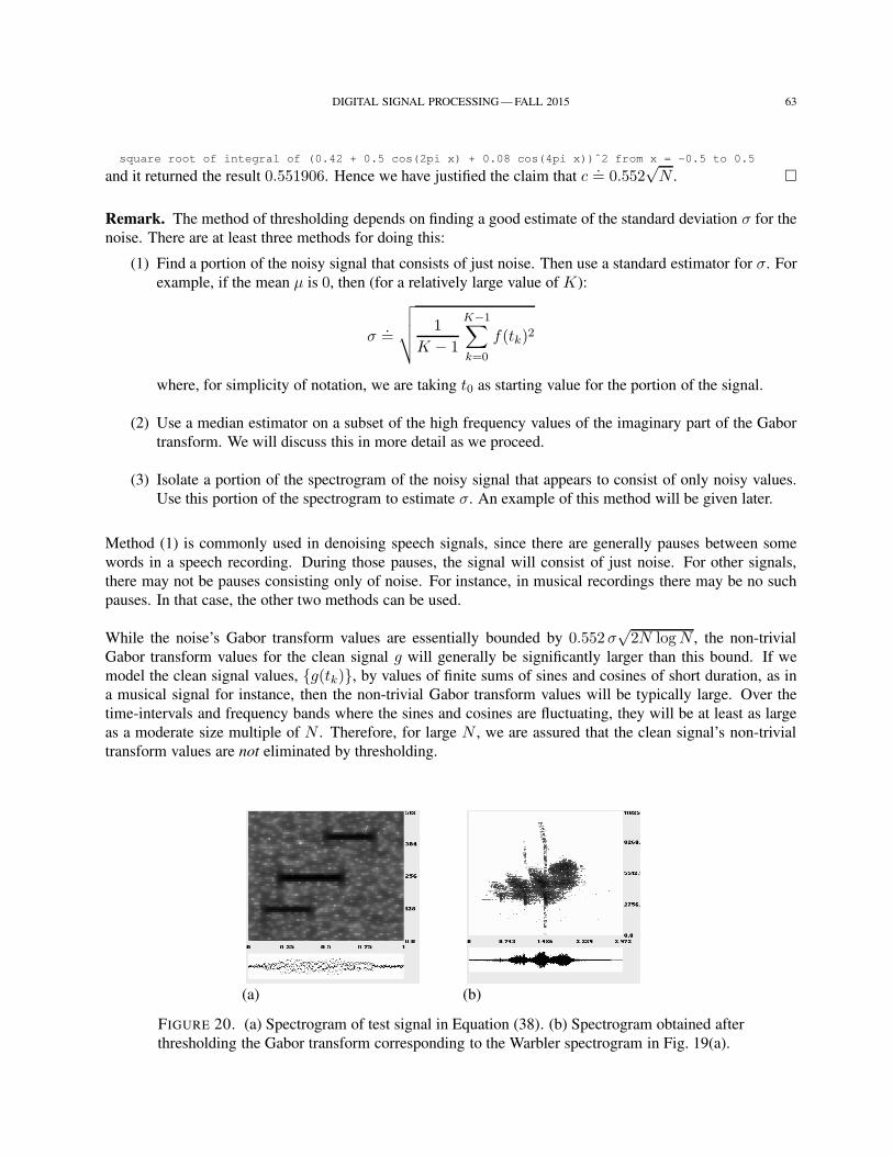
DIGITAL SIGNAL PROCESSING — FALL 2015 63
square root of integral of (0.42 + 0.5 cos(2pi x) + 0.08 cos(4pi x))ˆ2 from x = -0.5 to 0.5
and it returned the result 0.551906. Hence we have justified the claim that c.= 0.552
√N .
Remark. The method of thresholding depends on finding a good estimate of the standard deviation σ for the
noise. There are at least three methods for doing this:
(1) Find a portion of the noisy signal that consists of just noise. Then use a standard estimator for σ. For
example, if the mean µ is 0, then (for a relatively large value of K):
σ.=
√√√√ 1
K − 1
K−1∑
k=0
f(tk)2
where, for simplicity of notation, we are taking t0 as starting value for the portion of the signal.
(2) Use a median estimator on a subset of the high frequency values of the imaginary part of the Gabor
transform. We will discuss this in more detail as we proceed.
(3) Isolate a portion of the spectrogram of the noisy signal that appears to consist of only noisy values.
Use this portion of the spectrogram to estimate σ. An example of this method will be given later.
Method (1) is commonly used in denoising speech signals, since there are generally pauses between some
words in a speech recording. During those pauses, the signal will consist of just noise. For other signals,
there may not be pauses consisting only of noise. For instance, in musical recordings there may be no such
pauses. In that case, the other two methods can be used.
While the noise’s Gabor transform values are essentially bounded by 0.552σ√2N logN , the non-trivial
Gabor transform values for the clean signal g will generally be significantly larger than this bound. If we
model the clean signal values, g(tk), by values of finite sums of sines and cosines of short duration, as in
a musical signal for instance, then the non-trivial Gabor transform values will be typically large. Over the
time-intervals and frequency bands where the sines and cosines are fluctuating, they will be at least as large
as a moderate size multiple of N . Therefore, for large N , we are assured that the clean signal’s non-trivial
transform values are not eliminated by thresholding.
(a) (b)
FIGURE 20. (a) Spectrogram of test signal in Equation (38). (b) Spectrogram obtained after
thresholding the Gabor transform corresponding to the Warbler spectrogram in Fig. 19(a).
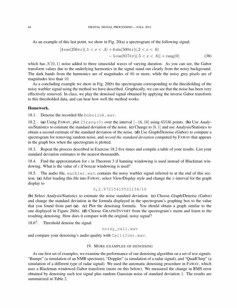
64 DIGITAL SIGNAL PROCESSING — FALL 2015
As an example of this last point, we show in Fig. 20(a) a spectrogram of the following signal:
[4 cos(256πx)(.1 < x < .4) + 6 sin(500πx)(.2 < x < .6)
− 5 cos(817πx)(.5 < x < .8)] + rang(0) (38)
which has N (0, 1) noise added to three sinusoidal waves of varying duration. As you can see, the Gabor
transform values due to the underlying harmonics in the signal stand out clearly from the noisy background.
The dark bands from the harmonics are of magnitudes of 80 or more, while the noisy grey pixels are of
magnitudes less than 10.
As a concluding example we show in Fig. 20(b) the spectrogram corresponding to the thresholding of the
noisy warbler signal using the method we have described. Graphically, we can see that the noise has been very
effectively removed. In class, we play the denoised signal obtained by applying the inverse Gabor transform
to this thresholded data, and can hear how well the method works.
Homework.
18.1. Denoise the recorded file bobolink.wav.
18.2. (a) Using FAWAV, plot 25rang(0) over the interval [−16, 16] using 65536 points. (b) Use Analy-
sis/Statistics to estimate the standard deviation of the noise. (c) Change to [0, 1] and use Analysis/Statistics to
obtain a second estimate of the standard deviation of the noise. (d) Use Graph/Denoise (Gabor) to compute a
spectrogram for removing random noise, and record the standard deviation computed by FAWAV that appears
in the graph box when the spectrogram is plotted.
18.3. Repeat the process described in Exercise 18.2 five times and compile a table of your results. List your
standard deviation estimates to the nearest thousandth.
18.4. Find the approximation for c in Theorem 3 if hanning windowing is used instead of Blackman win-
dowing. What is the value of c if boxcar windowing is used?
18.5. The audio file, warbler.wav, contains the noisy warbler signal referred to at the end of this sec-
tion. (a) After loading this file into FAWAV, select View/Display style and change the x-interval for the graph
display to
0,2.97215419501134/16
(b) Select Analysis/Statistics to estimate the noise standard deviation. (c) Choose Graph/Denoise (Gabor)
and change the standard deviation in the formula displayed in the spectrogram’s graphing box to the value
that you found from part (a). (c) Plot the denoising formula. You should obtain a graph similar to the
one displayed in Figure 20(b). (d) Choose GRAPH/INVERT from the spectrogram’s menu and listen to the
resulting denoising. How does it compare with the original, noisy signal?
18.6S . Threshold denoise the signal
noisy_call.wav
and compare your denoising’s audio quality with Call(Jim).wav.
19. MORE EXAMPLES OF DENOISING
As our first set of examples, we examine the performance of our denoising algorithm on a set of test signals:
“Bumps” (a simulation of an NMR spectrum), “Doppler” (a simulation of a radar signal), and “QuadChirp” (a
simulation of a different type of radar signal). We used the automatic denoising procedure in FAWAV, which
uses a Blackman windowed Gabor transform (more on this below). We measured the change in RMS error
obtained by denoising each test signal plus random Gaussian noise of standard deviation 1. The results are
summarized in Table 2.
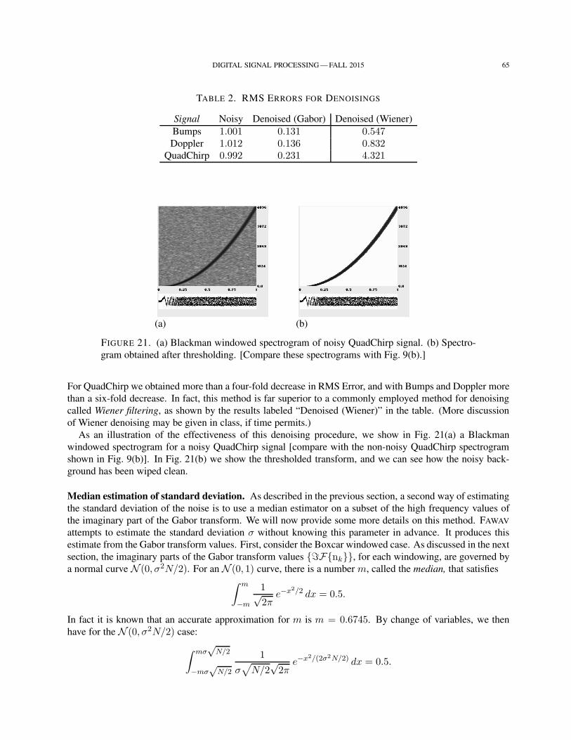
DIGITAL SIGNAL PROCESSING — FALL 2015 65
TABLE 2. RMS ERRORS FOR DENOISINGS
Signal Noisy Denoised (Gabor) Denoised (Wiener)
Bumps 1.001 0.131 0.547Doppler 1.012 0.136 0.832
QuadChirp 0.992 0.231 4.321
(a) (b)
FIGURE 21. (a) Blackman windowed spectrogram of noisy QuadChirp signal. (b) Spectro-
gram obtained after thresholding. [Compare these spectrograms with Fig. 9(b).]
For QuadChirp we obtained more than a four-fold decrease in RMS Error, and with Bumps and Doppler more
than a six-fold decrease. In fact, this method is far superior to a commonly employed method for denoising
called Wiener filtering, as shown by the results labeled “Denoised (Wiener)” in the table. (More discussion
of Wiener denoising may be given in class, if time permits.)
As an illustration of the effectiveness of this denoising procedure, we show in Fig. 21(a) a Blackman
windowed spectrogram for a noisy QuadChirp signal [compare with the non-noisy QuadChirp spectrogram
shown in Fig. 9(b)]. In Fig. 21(b) we show the thresholded transform, and we can see how the noisy back-
ground has been wiped clean.
Median estimation of standard deviation. As described in the previous section, a second way of estimating
the standard deviation of the noise is to use a median estimator on a subset of the high frequency values of
the imaginary part of the Gabor transform. We will now provide some more details on this method. FAWAV
attempts to estimate the standard deviation σ without knowing this parameter in advance. It produces this
estimate from the Gabor transform values. First, consider the Boxcar windowed case. As discussed in the next
section, the imaginary parts of the Gabor transform values ℑFnk, for each windowing, are governed by
a normal curve N (0, σ2N/2). For an N (0, 1) curve, there is a number m, called the median, that satisfies∫ m
−m
1√2π
e−x2/2 dx = 0.5.
In fact it is known that an accurate approximation for m is m = 0.6745. By change of variables, we then
have for the N (0, σ2N/2) case:
∫ mσ√
N/2
−mσ√
N/2
1
σ√
N/2√2π
e−x2/(2σ2N/2) dx = 0.5.
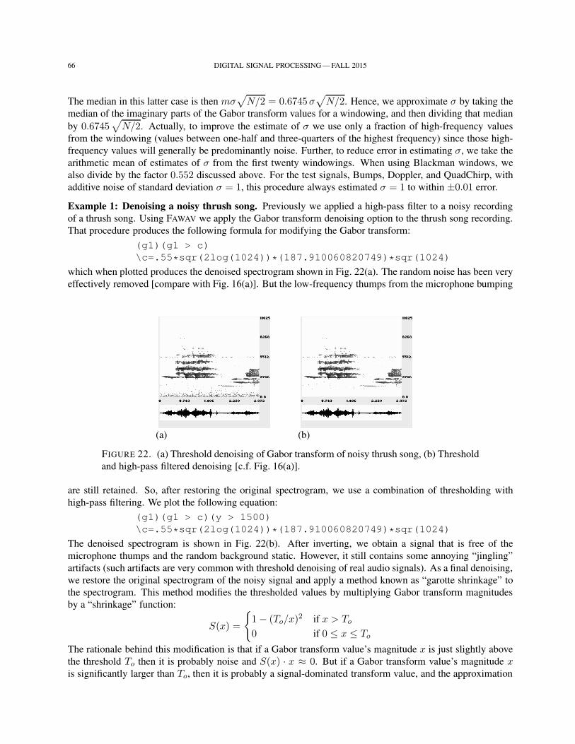
66 DIGITAL SIGNAL PROCESSING — FALL 2015
The median in this latter case is then mσ√
N/2 = 0.6745σ√
N/2. Hence, we approximate σ by taking the
median of the imaginary parts of the Gabor transform values for a windowing, and then dividing that median
by 0.6745√
N/2. Actually, to improve the estimate of σ we use only a fraction of high-frequency values
from the windowing (values between one-half and three-quarters of the highest frequency) since those high-
frequency values will generally be predominantly noise. Further, to reduce error in estimating σ, we take the
arithmetic mean of estimates of σ from the first twenty windowings. When using Blackman windows, we
also divide by the factor 0.552 discussed above. For the test signals, Bumps, Doppler, and QuadChirp, with
additive noise of standard deviation σ = 1, this procedure always estimated σ = 1 to within ±0.01 error.
Example 1: Denoising a noisy thrush song. Previously we applied a high-pass filter to a noisy recording
of a thrush song. Using FAWAV we apply the Gabor transform denoising option to the thrush song recording.
That procedure produces the following formula for modifying the Gabor transform:
(g1)(g1 > c)
\c=.55*sqr(2log(1024))*(187.910060820749)*sqr(1024)
which when plotted produces the denoised spectrogram shown in Fig. 22(a). The random noise has been very
effectively removed [compare with Fig. 16(a)]. But the low-frequency thumps from the microphone bumping
(a) (b)
FIGURE 22. (a) Threshold denoising of Gabor transform of noisy thrush song, (b) Threshold
and high-pass filtered denoising [c.f. Fig. 16(a)].
are still retained. So, after restoring the original spectrogram, we use a combination of thresholding with
high-pass filtering. We plot the following equation:
(g1)(g1 > c)(y > 1500)
\c=.55*sqr(2log(1024))*(187.910060820749)*sqr(1024)
The denoised spectrogram is shown in Fig. 22(b). After inverting, we obtain a signal that is free of the
microphone thumps and the random background static. However, it still contains some annoying “jingling”
artifacts (such artifacts are very common with threshold denoising of real audio signals). As a final denoising,
we restore the original spectrogram of the noisy signal and apply a method known as “garotte shrinkage” to
the spectrogram. This method modifies the thresholded values by multiplying Gabor transform magnitudes
by a “shrinkage” function:
S(x) =
1− (To/x)
2 if x > To
0 if 0 ≤ x ≤ To
The rationale behind this modification is that if a Gabor transform value’s magnitude x is just slightly above
the threshold To then it is probably noise and S(x) · x ≈ 0. But if a Gabor transform value’s magnitude xis significantly larger than To, then it is probably a signal-dominated transform value, and the approximation
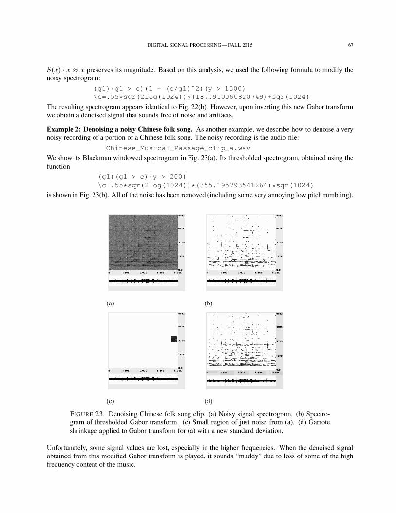
DIGITAL SIGNAL PROCESSING — FALL 2015 67
S(x) · x ≈ x preserves its magnitude. Based on this analysis, we used the following formula to modify the
noisy spectrogram:
(g1)(g1 > c)(1 - (c/g1)ˆ2)(y > 1500)
\c=.55*sqr(2log(1024))*(187.910060820749)*sqr(1024)
The resulting spectrogram appears identical to Fig. 22(b). However, upon inverting this new Gabor transform
we obtain a denoised signal that sounds free of noise and artifacts.
Example 2: Denoising a noisy Chinese folk song. As another example, we describe how to denoise a very
noisy recording of a portion of a Chinese folk song. The noisy recording is the audio file:
Chinese_Musical_Passage_clip_a.wav
We show its Blackman windowed spectrogram in Fig. 23(a). Its thresholded spectrogram, obtained using the
function
(g1)(g1 > c)(y > 200)
\c=.55*sqr(2log(1024))*(355.195793541264)*sqr(1024)
is shown in Fig. 23(b). All of the noise has been removed (including some very annoying low pitch rumbling).
(a) (b)
(c) (d)
FIGURE 23. Denoising Chinese folk song clip. (a) Noisy signal spectrogram. (b) Spectro-
gram of thresholded Gabor transform. (c) Small region of just noise from (a). (d) Garrote
shrinkage applied to Gabor transform for (a) with a new standard deviation.
Unfortunately, some signal values are lost, especially in the higher frequencies. When the denoised signal
obtained from this modified Gabor transform is played, it sounds “muddy” due to loss of some of the high
frequency content of the music.
68 DIGITAL SIGNAL PROCESSING — FALL 2015
To fix this problem, which is due to the rather high estimate of the standard deviation (σ ≈ 355), we need
a different estimate of the standard deviation. We find this new estimate using Method (3) in the Remark on
page 63. By examining the spectrogram in Fig. 23(a) we see that there is a region of the time-frequency plane,
shown in Fig. 23(c), that is mostly noise. To obtain the plot in Fig. 23(c) we used the following function:
g1(5.302<x<5.746)(2680<y<3263)
After performing an inverse Gabor transform, we then changed the x-range to 5.302, 5.746 and calculated the
standard deviation of the noisy signal. We got a new estimate of the variance: σ2 ≈ 8716. Since the signal
values were obtained using only a fraction of the possible frequencies, we adjust this variance estimate as
follows:
8716 · 5512.5
3263 − 2680≈ 82413
which is our new estimate of the noise variance. (More details on the theory behind this adjustment are given
in the optional section that begins on page 69; see especially page 71.) Our new estimate of the noise standard
deviation is the square root of this variance estimate, hence
σ ≈ 287.
Returning to the spectrogram window and restoring the noisy spectrogram of the full signal, we then plotted
the following garotte shrinkage
(g1)(g1 > c)(y > 200)(1 - (c/g1)ˆ2)
\c=.55*sqr(2log(1024))*(287)*sqr(1024)
which makes use of this new standard deviation estimate. The resulting plot is shown in Fig. 23(d). Com-
paring this denoised spectrogram with the one shown in Fig. 23(b), we see at first very little difference. That
indicates we now have an improved estimate of the noise standard deviation. Looking carefully, however,
there are some subtle differences. The spectrogram in (d) includes some additional details in harmonics. For
example, there is more structure to the harmonic that appears slightly below 4134 on the frequency axis and
just after 2.972 on the time axis. Listening to both denoisings, the second one is slightly more sharply defined,
due to better preservation of the high-frequency content of the music.
Homework.
The following three exercises explore method (3), described in the Remark on page 63, for estimating the
standard deviation of the noise. When using ANALYSIS/STATISTICS to estimate standard deviations, make
sure you also record the Number of samples reported, as this has a bearing on your answer to prob-
lem 19.3.
19.1. Plot the function 25rang(0) over the interval [−16, 16] using 65536 points. Use method (3) to
estimate the standard deviation of the noise from the Blackman windowed spectrogram using the following
rectangular regions:
(a)S 0 < x < 1 and 768 < y < 960,
(b) 0 < x < 1 and 768 < y < 864,
(c) 0 < x < 1 and 768 < y < 816,
(d) 0 < x < 1 and 768 < y < 1152.
19.2. Plot the function 25rang(0) over the interval [−16, 16] using 65536 points. Use method (3) to
estimate the standard deviation of the noise from the Blackman windowed spectrogram using the following
rectangular regions:
(a) 0 < x < 2 and 768 < y < 960,
(b) 0 < x < 0.5 and 768 < y < 960,
DIGITAL SIGNAL PROCESSING — FALL 2015 69
(c) 0 < x < 4 and 768 < y < 864,
(d) 0 < x < 2 and 768 < y < 864.
19.3S . Use your results from problems 19.1 and 19.2 to evaluate the accuracy of Method (3).
19.4. Denoise the noisy recording Chinese_Folk_Song_Clip_b.wav. Provide enough details about
your denoising method, including any formulas applied, so that someone else could duplicate your work.
19.5. Denoise the noisy recording Dan’s ’Bait’.wav. Provide enough details about your denoising
method, including any formulas applied, so that someone else could duplicate your work.
19.6. Denoise the noisy recording bobolink.wav. Note: If you use (g1>c)(1-(c/g1)ˆ2) to per-
form garotte shrinkage, you will get a Run error due to division by 0. Use the modified expression
(g1>c)(1-(c/u)ˆ2) \u=g1+(g1<c/2)
to avoid division by 0. Provide enough details about your denoising method, including any formulas applied,
so that someone else could duplicate your work.
MORE DETAILS ON ESTIMATING NOISE STANDARD DEVIATION [OPTIONAL]
In this section, we provide further discussion of Methods (2) and (3) in the Remark on page 63. Some of
the arguments here are more advanced, requiring more familiarity with probability theory and linear algebra,
so this section is optional.
Method (2). We begin with the following theorem, which says that an orthogonal transformation preserves
independent Gaussian random variables.
Theorem 4. Let x1, x2, . . . , xn be n mutually independent random variables, all of type N (0, σ2). Define
the random variables y1, y2, . . . , yn by
(x1, x2, . . . , xn)O−→ (y1, y2, . . . , yn)
where O is an n by n orthogonal matrix. Then y1, y2, . . . , yn are mutually independent and all of type
N (0, σ2).
Proof. The joint probability density function for (x1, x2, . . . , xn) is
p(x1, x2, . . . , xn) =1√2πσ
e−πx21/2σ
2 1√2πσ
e−πx22/2σ
2. . .
1√2πσ
e−πx2n/2σ
2.
The probability density can then be written in vector form, for x = (x1, x2, . . . , xn), as
p(x) dx =1
(2πσ2)n/2e−i2πx · x/2σ2
dx
where dx = dx1 dx2 . . . dxn. In vector form, we have xO−→ y. Since O−1 is also orthogonal—and therefore
preserves Euclidean distance and has a determinant of absolute value 1—we have
p(x) dx =1
(2πσ2)n/2e−i2πO−1y · O−1y/2σ2 |det(O−1)| dy
=1
(2πσ2)n/2e−i2πy · y/2σ2
dy
=1√2πσ
e−πy21/2σ2 1√
2πσe−πy22/2σ
2. . .
1√2πσ
e−πy2n/2σ2dy1 dy2 . . . dyn
70 DIGITAL SIGNAL PROCESSING — FALL 2015
Consequently, the joint p.d.f. for y = (y1, y2, . . . , yn) is
p(y1, y2, . . . , yn) =1√2πσ
e−πy21/2σ2 1√
2πσe−πy22/2σ
2. . .
1√2πσ
e−πy2n/2σ2.
Therefore, y1, y2, . . . , yn are mutually independent and all of type N (0, σ2), which completes the proof.
Now, in order to discuss method (2), we need the following Lemma.
Lemma 1. The matrix S =(
2√N
sin πkmN/2
)N/2−1, N/2−1
k=1,m=1is an orthogonal matrix.
Proof. If we take the dot product of the mth column with the jth column (for any choice of m and j), then
we get the following sum:
4
N
N/2−1∑
k=1
sinπkm
N/2sin
πkj
N/2.
Moreover, we have
sinπ(N − k)m
N/2sin
π(N − k)j
N/2= sin
πkm
N/2sin
πkj
N/2,
and sinπkm
N/2sin
πkj
N/2= 0 for k = 0 and k = N/2. Therefore,
N/2−1∑
k=1
sinπkm
N/2sin
πkj
N/2=
1
2
N−1∑
k=0
sinπkm
N/2sin
πkj
N/2
We then obtain
N/2−1∑
k=1
sinπkm
N/2sin
πkj
N/2=
1
2
N−1∑
k=0
sinπkm
N/2sin
πkj
N/2
=1
2
N−1∑
k=0
sin2πkm
Nsin
2πkj
N
=1
4
N−1∑
k=0
cos2πk(m− j)
N+
1
4
N−1∑
k=0
cos2πk(m+ j)
N.
But, we also have
1
4
N−1∑
k=0
cos2πk(m − j)
N=
1
4R
(N−1∑
k=0
ei2π(m−j)k/N
)
=
0 for m 6= j
N/4 for m = j
where the last equality follows from the proof of inversion for FFTs. Similarly, we have
1
4
N−1∑
k=0
cos2πk(m+ j)
N= 0.
DIGITAL SIGNAL PROCESSING — FALL 2015 71
Combining these results we obtain
4
N
N/2−1∑
k=1
sinπkm
N/2sin
πkj
N/2=
0 for m 6= j
1 for m = j
which proves that the columns of the matrix S are an orthonormal set. That proves that S is an orthogonal
matrix.
We now use Lemma 1 to prove that the imaginary part of the Fourier transform of the Gaussian noise
consists of two collections of independent Gaussian noise values.
ℑ(Xn) =
N−1∑
k=0
(−xk) sin2πkn
N
=
N/2−1∑
k=1
(−xk) sinπkn
N/2+
N−1∑
k=N/2+1
(−xk) sinπkn
N/2
=
N/2−1∑
k=1
(−xk) sinπkn
N/2+ (−1)n
N/2−1∑
k=1
(−xk+N/2) sinπkn
N/2
where the last line follows by change of index and sine addition identity. We therefore have
ℑ(Xn) =2√N
N/2−1∑
k=1
(−√N
2xk) sin
πkn
N/2+ (−1)n
2√N
N/2−1∑
k=1
(−√N
2xk+N/2) sin
πkn
N/2.
Thus, ℑ(Xn) = Yn + (−1)n Yn where Yn and Yn are the two random variables defined by
Yn =2√N
N/2−1∑
k=1
(−√N
2xk) sin
πkn
N/2, Yn =
2√N
N/2−1∑
k=1
(−√N
2xk+N/2) sin
πkn
N/2.
Thus, for n = 1, 2, . . . , N/2 − 1, Yn are N/2 − 1 random variables obtained by applying the matrix Sto the N/2 − 1 random variables −0.5
√N xk, k = 1, 2, . . . , N/2 − 1. It follows that Yn are mutu-
ally independent random variables of type N (0, Nσ2/4). Similarly, Yn are mutually independent random
variables of type N (0, Nσ2/4). Since Yn and Yn are transformations of disjoint sets of mutually inde-
pendent random variables, it follows that ℑ(Xn)N/2−1n=1 are all mutually independent random variables. By
Theorem 2 (or more specifically, property (B) on page 60), they all are type N (0, Nσ2/2). Moreover, since
ℑ(XN−n) = −ℑ(Xn), it follows that ℑ(Xn)N−1n=N/2+1 are also mutually independent random variables of
type N (0, Nσ2/2). Consequently, the median method of estimating σ/√2 can be applied to ℑ(Xn), as
described on page 65.
Method (3). We now turn to method (3). We will just sketch the main ideas. First, we recall Parseval’s
Equality:N−1∑
k=0
x2k =1
N
N−1∑
n=0
|Xn|2 (39)
where
Xn =
N−1∑
k=0
xke−i2πkn/N .
72 DIGITAL SIGNAL PROCESSING — FALL 2015
Here we are assuming that the window satisfies w(t) = 1, since the Gabor transform synthesis process will
remove the Blackman windowing when recovering the signal xk from the Gabor transform. From our
previous work, we have
E(|Xn|2
)= c2σ2 (40)
for each n. Because we are assuming boxcar windowing, due to removal of the window multiplication during
signal reconstruction, we will use c =√N in Equation (40). Thus, for each n, we have
E(|Xn|2
)= Nσ2.
This shows that in the reconstruction of xk:
xk =1
N
N∑
k=0
Xnei2πkn/N
each of the Xn values contributes equally to the standard deviation σ2 for xk.
Now, when we apply method (3), we only restrict to a subset of the transform values Xn. Consequently,
when estimating the standard deviation from a formula such as
σ ≈
√√√√ 1
K − 1
K−1∑
k=0
x2k
only a subset of the values Xn are contributing (equally) to the values x2k. Hence we obtain√√√√ 1
K − 1
K−1∑
k=0
x2k = rσ2
where r represents the percentage of values from Xn used in the Gabor synthesis of the values xk.
20. CORRELATION
In this section we describe the fundamental technique of correlation, with some basic applications to signal
detection and computing FFTs of arbitrary length. In the next section, we shall describe how correlations can
be used to zoom-in on portions of spectrograms, with improved resolution that avoids the blurring effects that
a simple zoom would create.
Definition [Correlation]. If hkN−1k=0 and gkN−1
k=0 are two sequences of N numbers, and gkN−1k=0 has
period N , then the correlation of h with g, denoted by (h : g), is the sequence of numbers (h : g)nN−1n=0
defined by
(h : g)n =
N−1∑
k=0
hkgk−n.
The normalized correlation of h with g is denoted by 〈h : g〉 and defined by
〈h : g〉n =(h : g)n∑N−1k=0 g2k
.
The normalized correlation is used for detecting the presence of translates of g as components of h, since
each signal gk−nN−1k=0 is a translate of g by the amount n. As a general rule, the normalized correlation
will have a maximum value of approximately 1 at index values n that mark locations where h contains a
component that is a translate of g. As an example, consider the test signal h generated by 1024 equally
spaced values, over the interval [−5, 5], of the piecewise defined function f(x):
2(-3<x<-2) + (1-abs(x))(abs(x)<1) -1(3<x<4)
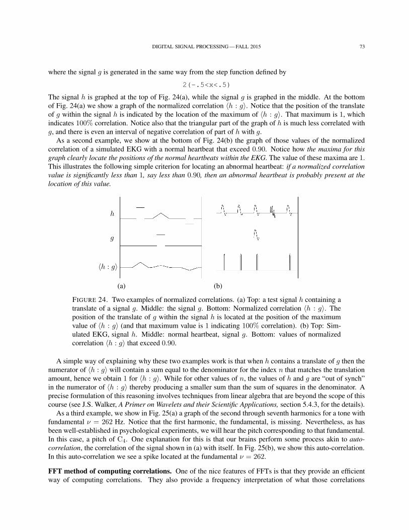
DIGITAL SIGNAL PROCESSING — FALL 2015 73
where the signal g is generated in the same way from the step function defined by
2(-.5<x<.5)
The signal h is graphed at the top of Fig. 24(a), while the signal g is graphed in the middle. At the bottom
of Fig. 24(a) we show a graph of the normalized correlation 〈h : g〉. Notice that the position of the translate
of g within the signal h is indicated by the location of the maximum of 〈h : g〉. That maximum is 1, which
indicates 100% correlation. Notice also that the triangular part of the graph of h is much less correlated with
g, and there is even an interval of negative correlation of part of h with g.
As a second example, we show at the bottom of Fig. 24(b) the graph of those values of the normalized
correlation of a simulated EKG with a normal heartbeat that exceed 0.90. Notice how the maxima for this
graph clearly locate the positions of the normal heartbeats within the EKG. The value of these maxima are 1.
This illustrates the following simple criterion for locating an abnormal heartbeat: if a normalized correlation
value is significantly less than 1, say less than 0.90, then an abnormal heartbeat is probably present at the
location of this value.
h
g
〈h : g〉
(a) (b)
FIGURE 24. Two examples of normalized correlations. (a) Top: a test signal h containing a
translate of a signal g. Middle: the signal g. Bottom: Normalized correlation 〈h : g〉. The
position of the translate of g within the signal h is located at the position of the maximum
value of 〈h : g〉 (and that maximum value is 1 indicating 100% correlation). (b) Top: Sim-
ulated EKG, signal h. Middle: normal heartbeat, signal g. Bottom: values of normalized
correlation 〈h : g〉 that exceed 0.90.
A simple way of explaining why these two examples work is that when h contains a translate of g then the
numerator of 〈h : g〉 will contain a sum equal to the denominator for the index n that matches the translation
amount, hence we obtain 1 for 〈h : g〉. While for other values of n, the values of h and g are “out of synch”
in the numerator of 〈h : g〉 thereby producing a smaller sum than the sum of squares in the denominator. A
precise formulation of this reasoning involves techniques from linear algebra that are beyond the scope of this
course (see J.S. Walker, A Primer on Wavelets and their Scientific Applications, section 5.4.3, for the details).
As a third example, we show in Fig. 25(a) a graph of the second through seventh harmonics for a tone with
fundamental ν = 262 Hz. Notice that the first harmonic, the fundamental, is missing. Nevertheless, as has
been well-established in psychological experiments, we will hear the pitch corresponding to that fundamental.
In this case, a pitch of C4. One explanation for this is that our brains perform some process akin to auto-
correlation, the correlation of the signal shown in (a) with itself. In Fig. 25(b), we show this auto-correlation.
In this auto-correlation we see a spike located at the fundamental ν = 262.
FFT method of computing correlations. One of the nice features of FFTs is that they provide an efficient
way of computing correlations. They also provide a frequency interpretation of what those correlations
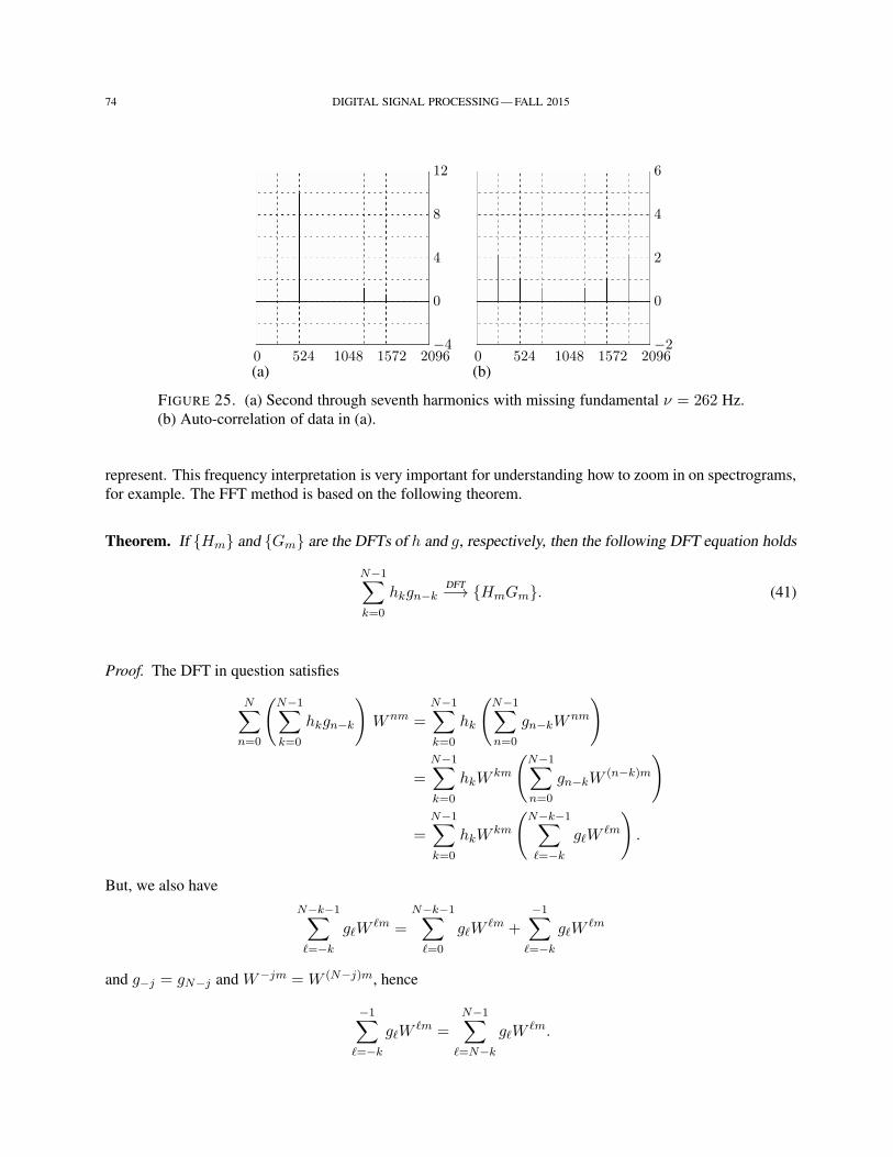
74 DIGITAL SIGNAL PROCESSING — FALL 2015
0 524 1048 1572 2096−4
0
4
8
12
(a)0 524 1048 1572 2096
−2
0
2
4
6
(b)
FIGURE 25. (a) Second through seventh harmonics with missing fundamental ν = 262 Hz.
(b) Auto-correlation of data in (a).
represent. This frequency interpretation is very important for understanding how to zoom in on spectrograms,
for example. The FFT method is based on the following theorem.
Theorem. If Hm and Gm are the DFTs of h and g, respectively, then the following DFT equation holds
N−1∑
k=0
hkgn−kDFT−→ HmGm. (41)
Proof. The DFT in question satisfies
N∑
n=0
(N−1∑
k=0
hkgn−k
)W nm =
N−1∑
k=0
hk
(N−1∑
n=0
gn−kWnm
)
=
N−1∑
k=0
hkWkm
(N−1∑
n=0
gn−kW(n−k)m
)
=N−1∑
k=0
hkWkm
(N−k−1∑
ℓ=−k
gℓWℓm
).
But, we also have
N−k−1∑
ℓ=−k
gℓWℓm =
N−k−1∑
ℓ=0
gℓWℓm +
−1∑
ℓ=−k
gℓWℓm
and g−j = gN−j and W−jm = W (N−j)m, hence
−1∑
ℓ=−k
gℓWℓm =
N−1∑
ℓ=N−k
gℓWℓm.
DIGITAL SIGNAL PROCESSING — FALL 2015 75
Therefore,
N−k−1∑
ℓ=−k
gℓWℓm =
N−k−1∑
ℓ=0
gℓWℓm +
N−1∑
ℓ=N−k
gℓWℓm
=
N−1∑
ℓ=0
gℓWℓm
and we then have
N∑
n=0
(N−1∑
k=0
hkgn−k
)W nm =
N−1∑
k=0
hkWkm
(N−1∑
ℓ=0
gℓWℓm
)
=
(N−1∑
k=0
hkWkm
)(N−1∑
ℓ=0
gℓWℓm
)
= HmGm
which completes the proof.
This theorem applies to correlations because the sum
N−1∑
k=0
hkgn−k
is the correlation (h : g) where g is the sequence defined by gk = g−k. We leave it as an exercise for the
reader to show that the DFT of g is Gn (when g is a real-valued signal). That is, we have the following
result:
(h : g)DFT−→ HmGm. (42)
This equation gives a simple three-step method for computing correlations: (1) FFT both sequences, (2)
multiply the values of one FFT by the complex conjugate of the other FFT, (3) apply an inverse FFT to the
product sequence from step (2). Because of the speed of FFTs, this method is significantly faster than directly
computing a correlation based on its original sum definition.
FFTs for arbitrary numbers of points. A nice application of the Theorem from this section is the calcu-
lation of FFTs for signals with any number N values (N need not be a power of 2). This method is called
Bluestein’s algorithm, or the chirp-z algorithm.
To derive Bluestein’s algorithm, we rewrite the DFT Fn as follows:
Fn =
N−1∑
k=0
fkWkn
=
N−1∑
k=0
fkWn2/2+k2/2−(n−k)2/2
= W n2/2N−1∑
k=0
fkWk2/2W−(n−k)2/2.
Now, define N to be the smallest power of 2 satisfying N ≥ 2N . Also define the sequence hkN−1k=0 by
hk =
fkW
k2/2 for k = 0, 1, 2, . . . , N − 1
0 for k = N, . . . , N − 1.
76 DIGITAL SIGNAL PROCESSING — FALL 2015
and the sequence gkN−1k=0 via
gn−k = W−(n−k)2/2
for k, n = 0, 1, . . . , N −1 and by periodic extension (period N ) for all other values of n and k. We then have
Fn = W n2/2N−1∑
k=0
hkgn−k
for n = 0, 1, . . . , N−1. By our theorem, the sum on the right of this equation can be computed by performing
two N -point FFTs, multiplying the values of those FFTs, and then performing an N -point inverse FFT.
Multiplying those final values by W n2/2 for n = 0, 1, . . . , N − 1, we obtain FnN−1k=0 , which is the required
DFT. Since Bluestein’s algorithm involves FFTs, it is a very fast algorithm for computing DFTs with arbitrary
numbers of points.
Homework.
20.1S . Verify that the DFT of g, for a real-valued sequence gk is Gm.
21. INTRODUCTION TO SCALOGRAMS
In this section we discuss a different method of describing the time-frequency content of a signal, one
that is analogous to a musical scale. This method, called a scalogram, is based on multiple correlations of
a signal with localized waves (with approximately constant frequencies arranged as divisions of octaves, as
in a musical scale). We begin by defining two types of scalograms that use damped cosine and damped sine
functions, and then define the best scalogram (the one we actually use) as a complex combination of these
two real-valued scalograms.
First, we define the Gabor cosine scalogram. This scalogram consists of correlations of a signal hk with
signals gk defined as follows:
gk = s−1C(tk/s)where s > 0 is a parameter value and C(t) is the function defined by
C(t) = w−1e−π(t/w)2 cos(2πηt/w)
for a width parameter w > 0 and frequency parameter η. Notice that the cosine factor in C has a frequency
of η/w. The width parameter controls the rate of damping to 0 of the bell-shaped graph of w−1e−π(t/w)2 .
The smaller the value of w, the faster it decays to 0. The correlations are done for discrete values sp of the
scale parameter s:
s = sp = 2−p/J , p = 0, 1, 2, . . . , I · J,where I is the number of octaves and J is the number of voices per octave.
As an example of how this works, consider the test signal hk obtained from 16 384 uniformly spaced
discrete values over the interval [−1, 1] of the following function:
(-.7 < x < -.4)sin(40pi x) + (-.3 < x < .3)cos(160 pi x)
+ (.6 < x < .9)sin(640 pi x)
In Fig. 26(a) we show a Blackman-windowed spectrogram of this signal. The dark bands corresponding to
the frequencies 20, 80, and 320 of the sinusoidals in the test signal are crowded together at the bottom of the
spectrogram. In Fig. 26(b) we show a Gabor cosine spectrogram (the whiter pixels represent larger positive
values, while the blacker pixels represent more negative values, the grey pixels represent values near 0). The
vertical axis represents multiples, by 1/sp, of the base frequency of 5. The frequencies of 20 = 5 · 22 and
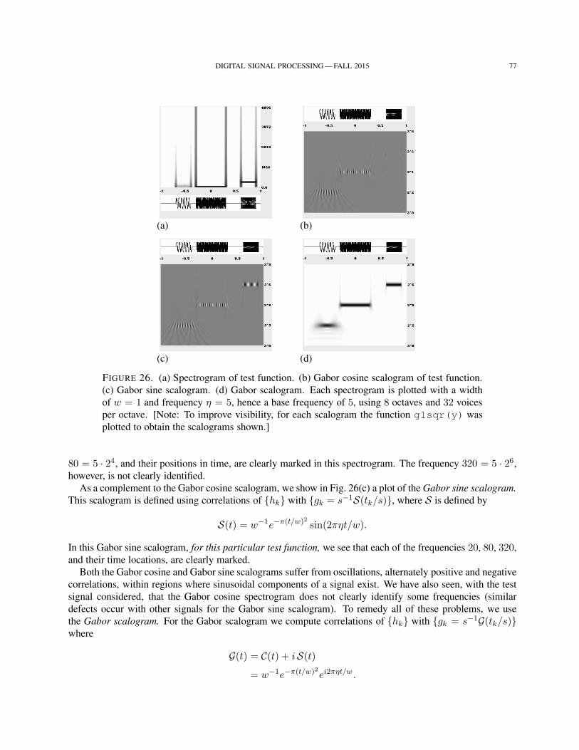
DIGITAL SIGNAL PROCESSING — FALL 2015 77
(a) (b)
(c) (d)
FIGURE 26. (a) Spectrogram of test function. (b) Gabor cosine scalogram of test function.
(c) Gabor sine scalogram. (d) Gabor scalogram. Each spectrogram is plotted with a width
of w = 1 and frequency η = 5, hence a base frequency of 5, using 8 octaves and 32 voices
per octave. [Note: To improve visibility, for each scalogram the function g1sqr(y) was
plotted to obtain the scalograms shown.]
80 = 5 · 24, and their positions in time, are clearly marked in this spectrogram. The frequency 320 = 5 · 26,
however, is not clearly identified.
As a complement to the Gabor cosine scalogram, we show in Fig. 26(c) a plot of the Gabor sine scalogram.
This scalogram is defined using correlations of hk with gk = s−1S(tk/s), where S is defined by
S(t) = w−1e−π(t/w)2 sin(2πηt/w).
In this Gabor sine scalogram, for this particular test function, we see that each of the frequencies 20, 80, 320,
and their time locations, are clearly marked.
Both the Gabor cosine and Gabor sine scalograms suffer from oscillations, alternately positive and negative
correlations, within regions where sinusoidal components of a signal exist. We have also seen, with the test
signal considered, that the Gabor cosine spectrogram does not clearly identify some frequencies (similar
defects occur with other signals for the Gabor sine scalogram). To remedy all of these problems, we use
the Gabor scalogram. For the Gabor scalogram we compute correlations of hk with gk = s−1G(tk/s)where
G(t) = C(t) + iS(t)= w−1e−π(t/w)2ei2πηt/w .
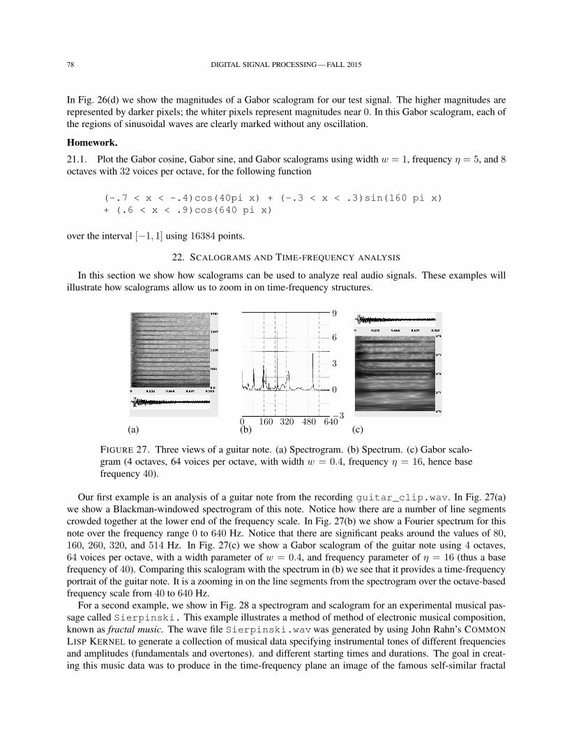
78 DIGITAL SIGNAL PROCESSING — FALL 2015
In Fig. 26(d) we show the magnitudes of a Gabor scalogram for our test signal. The higher magnitudes are
represented by darker pixels; the whiter pixels represent magnitudes near 0. In this Gabor scalogram, each of
the regions of sinusoidal waves are clearly marked without any oscillation.
Homework.
21.1. Plot the Gabor cosine, Gabor sine, and Gabor scalograms using width w = 1, frequency η = 5, and 8octaves with 32 voices per octave, for the following function
(-.7 < x < -.4)cos(40pi x) + (-.3 < x < .3)sin(160 pi x)
+ (.6 < x < .9)cos(640 pi x)
over the interval [−1, 1] using 16384 points.
22. SCALOGRAMS AND TIME-FREQUENCY ANALYSIS
In this section we show how scalograms can be used to analyze real audio signals. These examples will
illustrate how scalograms allow us to zoom in on time-frequency structures.
(a)0 160 320 480 640
−3
0
3
6
9
(b) (c)
FIGURE 27. Three views of a guitar note. (a) Spectrogram. (b) Spectrum. (c) Gabor scalo-
gram (4 octaves, 64 voices per octave, with width w = 0.4, frequency η = 16, hence base
frequency 40).
Our first example is an analysis of a guitar note from the recording guitar_clip.wav. In Fig. 27(a)
we show a Blackman-windowed spectrogram of this note. Notice how there are a number of line segments
crowded together at the lower end of the frequency scale. In Fig. 27(b) we show a Fourier spectrum for this
note over the frequency range 0 to 640 Hz. Notice that there are significant peaks around the values of 80,
160, 260, 320, and 514 Hz. In Fig. 27(c) we show a Gabor scalogram of the guitar note using 4 octaves,
64 voices per octave, with a width parameter of w = 0.4, and frequency parameter of η = 16 (thus a base
frequency of 40). Comparing this scalogram with the spectrum in (b) we see that it provides a time-frequency
portrait of the guitar note. It is a zooming in on the line segments from the spectrogram over the octave-based
frequency scale from 40 to 640 Hz.
For a second example, we show in Fig. 28 a spectrogram and scalogram for an experimental musical pas-
sage called Sierpinski. This example illustrates a method of method of electronic musical composition,
known as fractal music. The wave file Sierpinski.wavwas generated by using John Rahn’s COMMON
LISP KERNEL to generate a collection of musical data specifying instrumental tones of different frequencies
and amplitudes (fundamentals and overtones). and different starting times and durations. The goal in creat-
ing this music data was to produce in the time-frequency plane an image of the famous self-similar fractal
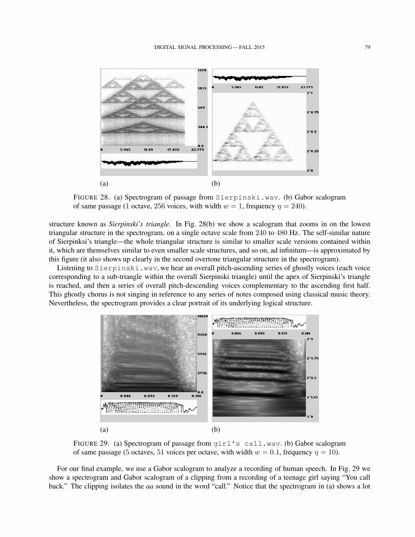
DIGITAL SIGNAL PROCESSING — FALL 2015 79
(a) (b)
FIGURE 28. (a) Spectrogram of passage from Sierpinski.wav. (b) Gabor scalogram
of same passage (1 octave, 256 voices, with width w = 1, frequency η = 240).
structure known as Sierpinski’s triangle. In Fig. 28(b) we show a scalogram that zooms in on the lowest
triangular structure in the spectrogram, on a single octave scale from 240 to 480 Hz. The self-similar nature
of Sierpinksi’s triangle—the whole triangular structure is similar to smaller scale versions contained within
it, which are themselves similar to even smaller scale structures, and so on, ad infinitum—is approximated by
this figure (it also shows up clearly in the second overtone triangular structure in the spectrogram).
Listening to Sierpinski.wav, we hear an overall pitch-ascending series of ghostly voices (each voice
corresponding to a sub-triangle within the overall Sierpinski triangle) until the apex of Sierpinski’s triangle
is reached, and then a series of overall pitch-descending voices complementary to the ascending first half.
This ghostly chorus is not singing in reference to any series of notes composed using classical music theory.
Nevertheless, the spectrogram provides a clear portrait of its underlying logical structure.
(a) (b)
FIGURE 29. (a) Spectrogram of passage from girl’s call.wav. (b) Gabor scalogram
of same passage (5 octaves, 51 voices per octave, with width w = 0.1, frequency η = 10).
For our final example, we use a Gabor scalogram to analyze a recording of human speech. In Fig. 29 we
show a spectrogram and Gabor scalogram of a clipping from a recording of a teenage girl saying “You call
back.” The clipping isolates the aa sound in the word “call.” Notice that the spectrogram in (a) shows a lot
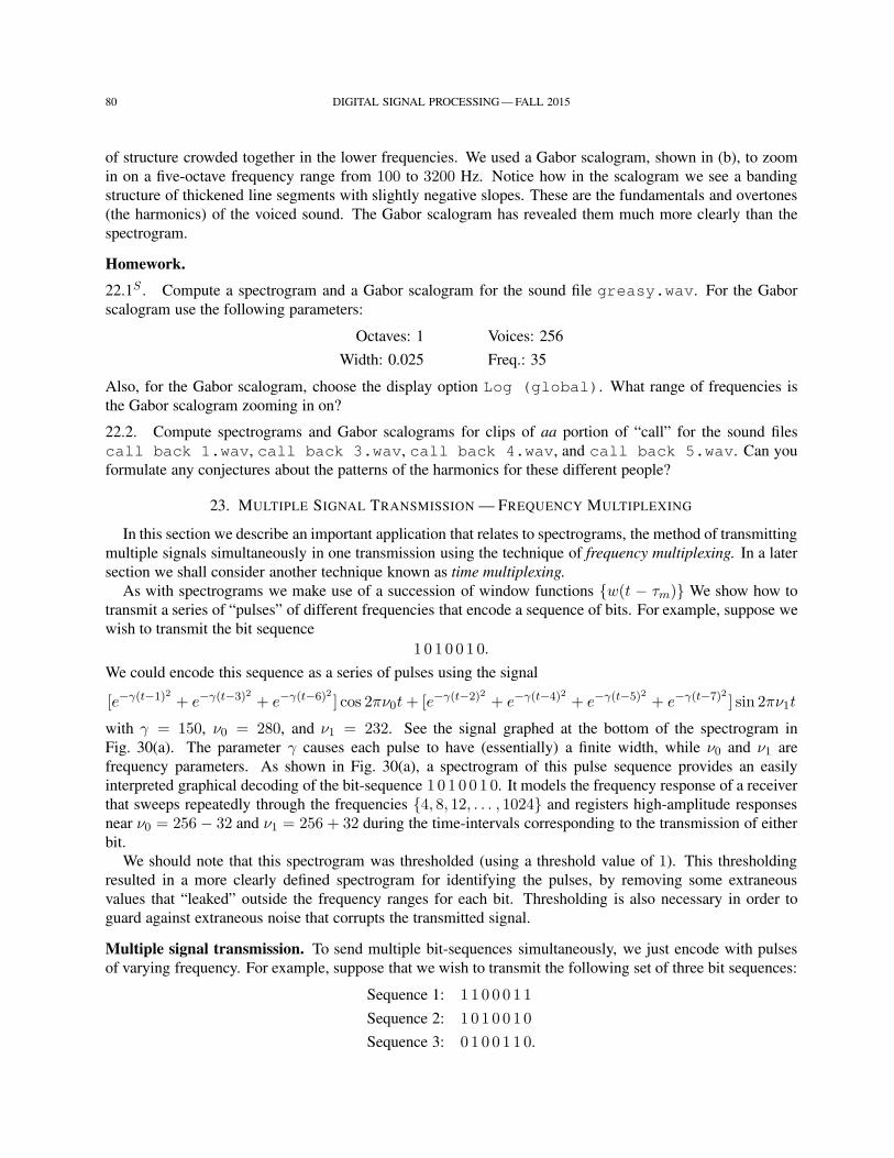
80 DIGITAL SIGNAL PROCESSING — FALL 2015
of structure crowded together in the lower frequencies. We used a Gabor scalogram, shown in (b), to zoom
in on a five-octave frequency range from 100 to 3200 Hz. Notice how in the scalogram we see a banding
structure of thickened line segments with slightly negative slopes. These are the fundamentals and overtones
(the harmonics) of the voiced sound. The Gabor scalogram has revealed them much more clearly than the
spectrogram.
Homework.
22.1S . Compute a spectrogram and a Gabor scalogram for the sound file greasy.wav. For the Gabor
scalogram use the following parameters:
Octaves: 1 Voices: 256
Width: 0.025 Freq.: 35
Also, for the Gabor scalogram, choose the display option Log (global). What range of frequencies is
the Gabor scalogram zooming in on?
22.2. Compute spectrograms and Gabor scalograms for clips of aa portion of “call” for the sound files
call back 1.wav, call back 3.wav, call back 4.wav, and call back 5.wav. Can you
formulate any conjectures about the patterns of the harmonics for these different people?
23. MULTIPLE SIGNAL TRANSMISSION — FREQUENCY MULTIPLEXING
In this section we describe an important application that relates to spectrograms, the method of transmitting
multiple signals simultaneously in one transmission using the technique of frequency multiplexing. In a later
section we shall consider another technique known as time multiplexing.
As with spectrograms we make use of a succession of window functions w(t − τm) We show how to
transmit a series of “pulses” of different frequencies that encode a sequence of bits. For example, suppose we
wish to transmit the bit sequence
1 0 1 0 0 1 0.
We could encode this sequence as a series of pulses using the signal
[e−γ(t−1)2 + e−γ(t−3)2 + e−γ(t−6)2 ] cos 2πν0t+ [e−γ(t−2)2 + e−γ(t−4)2 + e−γ(t−5)2 + e−γ(t−7)2 ] sin 2πν1t
with γ = 150, ν0 = 280, and ν1 = 232. See the signal graphed at the bottom of the spectrogram in
Fig. 30(a). The parameter γ causes each pulse to have (essentially) a finite width, while ν0 and ν1 are
frequency parameters. As shown in Fig. 30(a), a spectrogram of this pulse sequence provides an easily
interpreted graphical decoding of the bit-sequence 1 0 1 0 0 1 0. It models the frequency response of a receiver
that sweeps repeatedly through the frequencies 4, 8, 12, . . . , 1024 and registers high-amplitude responses
near ν0 = 256 − 32 and ν1 = 256 + 32 during the time-intervals corresponding to the transmission of either
bit.
We should note that this spectrogram was thresholded (using a threshold value of 1). This thresholding
resulted in a more clearly defined spectrogram for identifying the pulses, by removing some extraneous
values that “leaked” outside the frequency ranges for each bit. Thresholding is also necessary in order to
guard against extraneous noise that corrupts the transmitted signal.
Multiple signal transmission. To send multiple bit-sequences simultaneously, we just encode with pulses
of varying frequency. For example, suppose that we wish to transmit the following set of three bit sequences:
Sequence 1: 1 1 0 0 0 1 1
Sequence 2: 1 0 1 0 0 1 0
Sequence 3: 0 1 0 0 1 1 0.
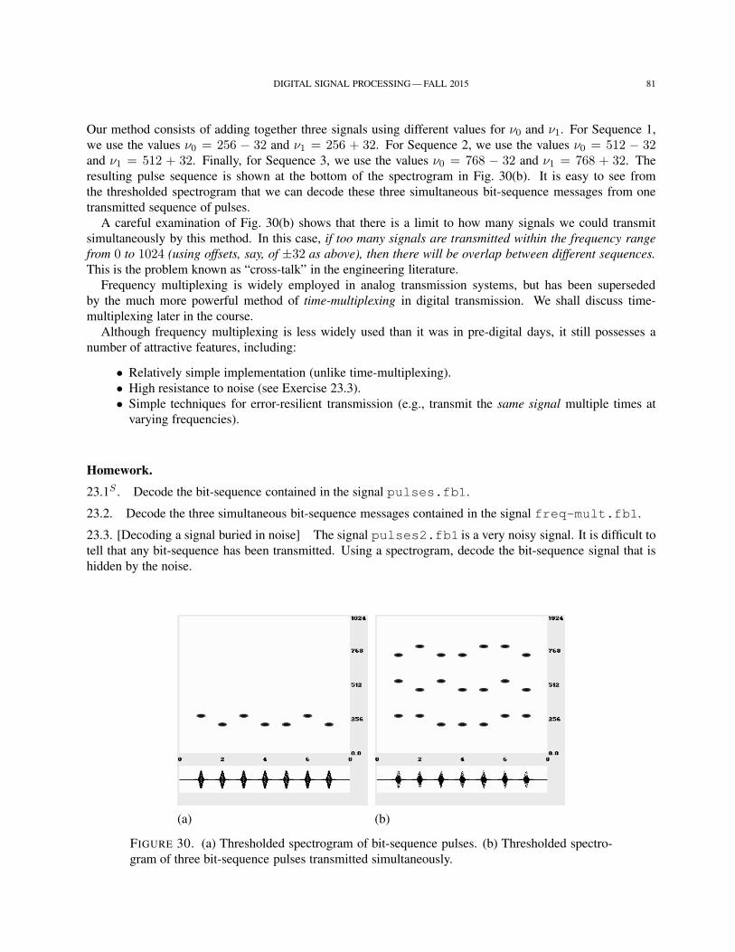
DIGITAL SIGNAL PROCESSING — FALL 2015 81
Our method consists of adding together three signals using different values for ν0 and ν1. For Sequence 1,
we use the values ν0 = 256 − 32 and ν1 = 256 + 32. For Sequence 2, we use the values ν0 = 512 − 32and ν1 = 512 + 32. Finally, for Sequence 3, we use the values ν0 = 768 − 32 and ν1 = 768 + 32. The
resulting pulse sequence is shown at the bottom of the spectrogram in Fig. 30(b). It is easy to see from
the thresholded spectrogram that we can decode these three simultaneous bit-sequence messages from one
transmitted sequence of pulses.
A careful examination of Fig. 30(b) shows that there is a limit to how many signals we could transmit
simultaneously by this method. In this case, if too many signals are transmitted within the frequency range
from 0 to 1024 (using offsets, say, of ±32 as above), then there will be overlap between different sequences.
This is the problem known as “cross-talk” in the engineering literature.
Frequency multiplexing is widely employed in analog transmission systems, but has been superseded
by the much more powerful method of time-multiplexing in digital transmission. We shall discuss time-
multiplexing later in the course.
Although frequency multiplexing is less widely used than it was in pre-digital days, it still possesses a
number of attractive features, including:
• Relatively simple implementation (unlike time-multiplexing).
• High resistance to noise (see Exercise 23.3).
• Simple techniques for error-resilient transmission (e.g., transmit the same signal multiple times at
varying frequencies).
Homework.
23.1S . Decode the bit-sequence contained in the signal pulses.fb1.
23.2. Decode the three simultaneous bit-sequence messages contained in the signal freq-mult.fb1.
23.3. [Decoding a signal buried in noise] The signal pulses2.fb1 is a very noisy signal. It is difficult to
tell that any bit-sequence has been transmitted. Using a spectrogram, decode the bit-sequence signal that is
hidden by the noise.
(a) (b)
FIGURE 30. (a) Thresholded spectrogram of bit-sequence pulses. (b) Thresholded spectro-
gram of three bit-sequence pulses transmitted simultaneously.
82 DIGITAL SIGNAL PROCESSING — FALL 2015
PART 3. FOURIER TRANSFORM
24. INTRODUCTION
Fourier transforms are used for frequency analysis of non-periodic functions. Suppose f is a non-periodic
function defined for all real values. We now derive the definition of the Fourier transform of f .
Our derivation will begin with the Fourier series for fL, the 2L-periodic function which equals f on the
interval [−L,L]. Notice that, for any fixed value of x, we have fL(x) → f(x) as L → ∞ [since for all values
of L > |x| we will have fL(x) = f(x)].Now, expand fL in a 2L-period Fourier series (assuming convergence):
fL(x) =
∞∑
n=−∞cne
i2πnx/2L
with
cn =1
2L
∫ L
−Lf(t)e−i2πnt/2L dt.
Substituting the formula for cn into the Fourier series, we obtain
fL(x) =
∞∑
n=−∞
(1
2L
∫ L
−Lf(t)e−i2πnt/2L dt
)ei2πnx/2L.
Defining un = n/2L, which are the frequencies for this Fourier series, and ∆u = un+1 − un = 1/2L, we
then have
fL(x) =
∞∑
n=−∞
(∫ L
−Lf(t)e−i2πunt dt
)ei2πunx∆u. (43)
If we now let L → ∞, then the left side of (43) tends to f(x). The integral∫ L−L on its right side tends to
∫∞−∞, and (by analogy with Riemann sum limits for definite integrals), we expect that the sum
∞∑
n=−∞with ∆u
as factor will tend to an integral∫∞−∞ with differential du as factor. Letting L → ∞, we are thus led to write
f(x) =
∫ ∞
−∞
(∫ ∞
−∞f(t)e−i2πut dt
)ei2πux du. (44)
Notice that ∆u → 0 as L → ∞, so the discrete frequencies un = n/2L are replaced by a continuous
frequency variable u. Thus u is the frequency of each complex exponential ei2πux in the outer integral on the
right side of (44).
Based on (44), we make the following definition of the Fourier transform. In this definition, we refer to a
function f for which∫∞−∞ |f(x)| dx is finite (converges) as absolutely integrable.
Definition. For an absolutely integrable function f , its Fourier transform f is a function of frequency udefined by
f(u) =
∫ ∞
−∞f(t)e−i2πut dt.
Requiring f to be absolutely integrable ensures that the integral∫∞−∞ f(t)e−i2πut dt converges, for each value
DIGITAL SIGNAL PROCESSING — FALL 2015 83
of u. In fact, by the comparison test for convergence of integrals, we have:
∣∣∣∣∫ ∞
−∞f(t)e−i2πut dt
∣∣∣∣ ≤∫ ∞
−∞
∣∣f(t)e−i2πut∣∣ dt
=
∫ ∞
−∞|f(t)| dt < ∞.
Thus,∫∞−∞ f(t)e−i2πut dt converges (absolutely) for each value of u. Notice that we have also shown that f
is bounded, with
|f(u)| ≤ ‖f‖1for all u (where ‖f‖1 is the constant
∫∞−∞ |f(t)| dt).
Based on our definition of Fourier transform, we can rewrite (44) as
f(x) =
∫ ∞
−∞f(u)ei2πux du. (45)
Formula (45) is known as the Fourier transform inversion formula.
Note: We do not regard (45) as mathematically proved at this point, since we derived it by making a loose
analogy between an infinite Riemann sum converging to an infinite integral with finite Riemann sums con-
verging to finite integrals. Later we shall discuss the mathematical justification of (45) for a wide variety of
functions.
Example. Let f be defined by
f(x) =
1 if |x| < 1/2
1/2 if x = ±1/2
0 if |x| > 1/2.
We shall call f by the name rec (for rectangle function). Its Fourier transform, rec, is calculated as follows.
First, suppose u 6= 0. Then
rec(u) =
∫ ∞
−∞rec(t)e−i2πut dt
=
∫ 1/2
−1/2cos(2πut) dt− i
∫ 1/2
−1/2sin(2πut) dt
= 2
∫ 1/2
0cos(2πut) dt
=2 sin(2πut)
2πu
∣∣∣∣t=1/2
t=0
=sinπu
πu.
Thus, for u 6= 0, we have
rec(u) =sinπu
πu.
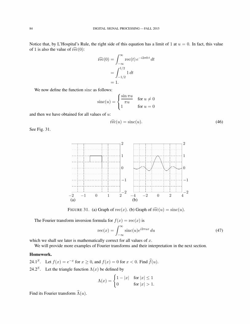
84 DIGITAL SIGNAL PROCESSING — FALL 2015
Notice that, by L’Hospital’s Rule, the right side of this equation has a limit of 1 at u = 0. In fact, this value
of 1 is also the value of rec(0):
rec(0) =
∫ ∞
−∞rec(t) e−i2π0 t dt
=
∫ 1/2
−1/21 dt
= 1.
We now define the function sinc as follows:
sinc(u) =
sinπu
πufor u 6= 0
1 for u = 0
and then we have obtained for all values of u:
rec(u) = sinc(u). (46)
See Fig. 31.
−2 −1 0 1 2−2
−1
0
1
2
(a)−4 −2 0 2 4
−2
−1
0
1
2
(b)
FIGURE 31. (a) Graph of rec(x). (b) Graph of rec(u) = sinc(u).
The Fourier transform inversion formula for f(x) = rec(x) is
rec(x) =
∫ ∞
−∞sinc(u)ei2πux du (47)
which we shall see later is mathematically correct for all values of x.
We will provide more examples of Fourier transforms and their interpretation in the next section.
Homework.
24.1S . Let f(x) = e−x for x ≥ 0, and f(x) = 0 for x < 0. Find f(u).
24.2S . Let the triangle function Λ(x) be defined by
Λ(x) =
1− |x| for |x| ≤ 1
0 for |x| > 1.
Find its Fourier transform Λ(u).
DIGITAL SIGNAL PROCESSING — FALL 2015 85
24.3. Use real-valued Fourier series to derive the following result:
f(x) = 2
∫ ∞
0
(∫ ∞
−∞f(t) cos 2πu(x− t) dt
)du
which is Fourier’s Integral Theorem.
24.4. Prove that if f is an even, absolutely integrable function, then
f(u) = 2
∫ ∞
0f(t) cos(2πut) dt.
24.5. For f(x) = e−|x|, find f(u).
25. INTERPRETATION OF FOURIER TRANSFORMS AND MORE EXAMPLES
We shall compute some more examples of Fourier transforms, but before doing so it may be of some help
to further discuss formulas (45) and (47) from the preceding section.
Formula (47) expresses rec(x) as an integral over all frequencies u of the functions sinc(u)ei2πux. For any
given value of u, sinc(u) is the amplitude of the wave sinc(u)ei2πux of frequency u. For example, suppose
u = 9/2. we then have sinc(u)ei2πux =2
9πei9πx, which is a wave of frequency 9/2 and amplitude
2
9π.
Formula (47) says that by superpositioning (via an integral) all waves of amplitude sinc(u) and frequency u,
we obtain rec(x).
Likewise, formula (45) says that to produce f(x) we superposition all waves of amplitude f(u) and fre-
quency u (i.e., form the integral∫∞−∞ f(u)ei2πux du). We shall see later that for an absolutely integrable,
regular function f(x) this statement is correct. Formula (45) does hold for such functions.
Finally, we mention an important analogy between Fourier transform inversion and summation of Fourier
series. When considering Fourier series, we view them as limits of partial sums SN (x). Each partial sum
(period 2a)
SN (x) =
N∑
n=−N
cnei2πnx/2a
is a sum of complex exponentials with frequencies n/2a ranging from −N/2a to N/2a and separated by
increments of 1/2a. We write, when convergence holds,
f(x) =
∞∑
n=−∞cne
i2πnx/2a
= limN→∞
SN (x)
and we note that the amplitude of each complex exponential is cn =1
2a
∫ a
−af(x)e−i2πnx/2a dx. In consider-
ing Fourier transforms we look at things in a similar way. Defining SL(x) by
SL(x) =
∫ L
−Lf(u)ei2πux du,
86 DIGITAL SIGNAL PROCESSING — FALL 2015
we shall see later that f(x) is (under certain conditions) a limit of SL(x) as L → ∞:
f(x) = limL→∞
SL(x)
=
∫ ∞
−∞f(u)ei2πux du. (48)
The function SL(x), called the partial sum integral, is a continuous sum (integral) of exponentials of all
frequencies u ranging from −L to L. Thus we see that there is an analogy between the partial sums in
Fourier series and the partial sum integrals in Fourier transform inversion.
We now compute a couple more examples of Fourier transforms.
Example 1. We find the Fourier transform of f(x) = e−2π|x|. We have
f(u) =
∫ ∞
−∞e−2π|x|e−i2πux dx
=
∫ ∞
−∞e−2π|x| cos(2πux) dx− i
∫ ∞
−∞e−2π|x| sin(2πux) dx
= 2
∫ ∞
0e−2πx cos(2πux) dx.
We now perform two integration by parts, obtaining
f(u) = 2
∫ ∞
0e−2πx cos(2πux) dx
= e−2πx 2 sin 2πux
2πu
∣∣∣∣x→∞
x=0
− 1
πe−2πx cos 2πux
u2
∣∣∣∣x→∞
x=0
− 2
∫ ∞
0
e−2πx cos 2πux
u2dx
=1
π
1
u2− 2
u2
∫ ∞
0e−2πx cos 2πux dx
=1
π
1
u2− 1
u2f(u).
Therefore,(1 +
1
u2
)f(u) =
1
π
1
u2.
Hence
f(u) =1
π
1
u2u2
u2 + 1
and that yields
f(u) =1
π
1
u2 + 1.
Introducing the notation f(x)F−→ f(u) to indicate the Fourier transform operation, we have found that
e−2π|x| F−→ 1
π
1
u2 + 1.
DIGITAL SIGNAL PROCESSING — FALL 2015 87
Example 2. In this example, we compute the Fourier transform of the Gaussian function e−πx2. This function
describes a normal probability curve of mean 0 and standard deviation 1/√2π. In fact, we have
∫ ∞
−∞e−πx2
dx = 1.
To see this, we let I be the value of the integral on the left, and then compute (using a change to polar
coordinates):
I2 =
∫ ∞
−∞e−πx2
dx ·∫ ∞
−∞e−πy2 dy
=
∫ ∞
−∞
∫ ∞
−∞e−π(x2+y2) dx dy
=
∫ 2π
0
∫ ∞
0e−πr2r dr dθ
=
∫ 2π
0
[−1
2πe−πr2
∣∣∣∣r→∞
r=0
]dθ
=
∫ 2π
0
1
2πdθ
= 1.
Thus, I2 = 1. Since we clearly have I > 0, we conclude that I = 1.
Now, we will show that e−πx2 F−→ e−πu2. In other words, the Fourier transform of this normal probability
curve is exactly the same normal probability curve, as a function of u, with mean 0 and standard deviation
1/√2π. Using the fact that e−πx2
is an even function, we obtain
f(u) = 2
∫ ∞
0e−πx2
cos 2πux dx.
Now, calculate the derivative of both sides
df
du=
d
du
∫ ∞
02e−πx2
cos 2πux dx
=
∫ ∞
02e−πx2
(−2πx) sin 2πux dx
where we have differentiated under the integral sign (treating x like a constant when differentiating by u).
[This differentiation under the integral sign is justified in Fourier Analysis, Section 6.2.]
We can now do the last integral above by integrating by parts:∫ ∞
02e−πx2
(−2πx) sin 2πux dx = 2e−πx2sin 2πux
∣∣∣x→∞
x=0−∫ ∞
04πu cos 2πux e−πx2
dx
= −2πu
(2
∫ ∞
0cos 2πux e−πx2
dx
)
= −2πuf(u).
Thus, we have the differential equation
df
du= −2πuf(u).
88 DIGITAL SIGNAL PROCESSING — FALL 2015
To solve this differential equation, we divide both sides by f(u) and integrate, obtaining
∫df/du
f(u)du =
∫−2πu du.
Hence
ln |f(u)| = −πu2 + C.
Therefore,
|f(u)| = eC e−πu2
so f(u) = ±eC e−πu2which we express as f(u) = Ae−πu2
for some constant A. But, by substituting u = 0,
we get f(0) = A and we also know that
f(0) =
∫ ∞
−∞e−πx2
e−i2π0x dx
=
∫ ∞
−∞e−πx2
dx
= 1.
Thus, A = 1 and we conclude that f(u) = e−πu2.
We summarize all of the examples of Fourier transforms that we have found so far:
rec(x)F−→ sinc(u)
Λ(x)F−→ sinc2(u)
e−2π|x| F−→ 1
π
1
u2 + 1
e−πx2 F−→ e−πu2
Computer algebra calculation of Fourier transforms. We can use WolframAlpha to calculate some Fourier
transforms. For example, we will show how WolframAlpha can be used to compute the transforms found in
Examples 1 and 2 above. First, for Example 1, the WolframAlpha calculations are as follows:
Text box: integrate eˆ(-2pi|x|)eˆ(-i2pi ux) from x=-infinity to infinity
Definite integral:
∫ ∞
−∞
1
e2π|x| ei2πuxdx =
1
πu2 + π
and that confirms the result we found for the transform in Example 1. Second, for Example 2, we tried a
similar approach as Example 1, as follows:
Text box: integrate eˆ(-pi xˆ2)eˆ(-i2pi ux) from x=-infinity to infinity
Definite integral:
∫ ∞
−∞
1
eπx2 ei2πuxdx
Standard computation time exceeded. . . Try again with additional computation time ≫
Clicking on the icon ≫ brought up a pop-up window that said that WolframAlpha Pro would provide three
times more computation time. Not being sure whether that would be enough time, and wishing to stay with
only the free version, this invitation to subscribe to WolframAlpha Pro was declined. Nevertheless, there is a
DIGITAL SIGNAL PROCESSING — FALL 2015 89
way to compute the transform f(u) more efficiently with WolframAlpha. In Example 2 above, we found that
f(u) = 2∫∞0 e−πx2
cos 2πux dx. Using that fact, WolframAlpha gave us
Text box: integrate 2eˆ(-pi xˆ2) cos(2pi ux) from x=0 to infinity
Definite integral:
∫ ∞
−∞
2 cos(2π(ux))
eπx2dx = e−πu
2
which matches the result we found above.
Homework.
25.1S . Given f(x) = e−|x|, find f(u).
25.2. Given f(x) = e−x2, find f(u).
25.3. Given
f(x) =
1− |x|/2 for |x| ≤ 2
0 for |x| > 2
find f(u).
25.4. Given
f(x) =
1 for 0 < x < 1
0 for x < 0 or x > 1
find f(u).
26. BASIC PROPERTIES OF FOURIER TRANSFORMS
There are four essential properties of Fourier transforms which are described by the following theorem.
Theorem. Given f(x)F−→ f(u) and g(x)
F−→ g(u), the following properties hold:
Linearity: For all constants α and β,
αf(x) + βg(x)F−→ αf(u) + βg(u).
Shifting: For each real constant c,
f(x− c)F−→ f(u)e−i2πcu.
Scaling: For every positive constant ρ,
f(ρx)F−→ 1
ρf
(u
ρ
), and f
(x
ρ
)F−→ ρf(ρu).
Modulation: For each real constant c,
f(x)ei2πcxF−→ f(u− c)
f(x) cos 2πcxF−→ 1
2f(u− c) +
1
2f(u+ c)
f(x) sin 2πcxF−→ 1
2if(u− c)− 1
2if(u+ c).
90 DIGITAL SIGNAL PROCESSING — FALL 2015
Proof. Linearity follows from the linearity of integrals:
αf(x) + βg(x)F−→∫ ∞
−∞[αf(x) + βg(x)]e−i2πux dx
= α
∫ ∞
−∞f(x)e−i2πux dx+ β
∫ ∞
−∞g(x)e−i2πux dx
= αf(u) + βg(u).
To prove the shifting property, we make a simple change of variable (t = x− c, dt = dx):
f(x− c)F−→∫ ∞
−∞f(x− c)e−i2πux dx
=
∫ ∞
−∞f(t)e−i2πu(t+c) dt
=
∫ ∞
−∞f(t)e−i2πut e−i2πuc dt
=
∫ ∞
−∞f(t)e−i2πut dt e−i2πuc
= f(u)e−i2πcu.
To prove the scaling property, we make another simple change of variable (t = ρx, dt = ρdx):
f(ρx)F−→∫ ∞
−∞f(ρx)e−i2πux dx
=
∫ ∞
−∞f(t)e−i2πu(t/ρ) 1
ρdt
=1
ρ
∫ ∞
−∞f(t)e−i2π(u/ρ)t dt
=1
ρf
(u
ρ
).
Finally, we prove the first modulation property as follows:
f(x)ei2πcxF−→∫ ∞
−∞f(x)ei2πcx e−i2πux dx
=
∫ ∞
−∞f(x)e−i2π(u−c)x dx
= f(u− c).
Proving the remaining two modulation properties is left to the reader as an exercise.
Example 1. We find the Fourier transform of
f(x) =
1 for 3 < x < 7
0 for x < 3 or x > 7.
By examining the graph of f we conclude that
f(x) = rec
(x− 5
4
).
DIGITAL SIGNAL PROCESSING — FALL 2015 91
By the shifting property we have
rec
(x− 5
4
)F−→ rec(x/4)(u) e−i2π5u
and by the scaling property
rec(x/4)(u) = 4 sinc(4u).
Thus,
f(u) = 4 sinc(4u) e−i10πu.
Example 2. We find the Fourier transform of
f(x) =
sin 12πx when |x| < 4
0 when |x| ≥ 4.
First, we observe that
f(x) =
1 when |x| < 4
0 when |x| ≥ 4
sin 12πx
= rec(x8
)sin 12πx.
Second, by the scaling property,
rec(x8
) F−→ 8 sinc(8u)
and by the modulation and linearity properties
f(x) =1
2irec(x8
)ei2π 6u − 1
2irec(x8
)e−i2π 6u
F−→ 1
2i8 sinc(8(u − 6)) − 1
2i8 sinc(8(u + 6)).
Thus, f(u) = 4i sinc(8u + 48) − 4i sinc(8u− 48).
Example 3. For each ρ > 0, we find the Fourier transform of fρ(x) = πρ−1 e−2π|x|/ρ. By the scaling and
linearity properties, we have
fρ(x) =π
ρe−2π|x/ρ| F−→ π
ρρ1
π
1
(ρu)2 + 1.
Thus,
fρ(u) =1
ρ2u2 + 1.
Remark. For this last example, we note that as ρ → 0+, we have fρ(u) → 1 for all u. But,
fρ(x) →∞ for x = 0
0 for x 6= 0
and, for every ρ > 0, ∫ ∞
−∞fρ(x) dx = 1.
Because of these last two facts, it is customary to write
limρ→0+
fρ(x) = δ(x)
92 DIGITAL SIGNAL PROCESSING — FALL 2015
where δ(x) is the Dirac delta function. By the limit fρ(u) → 1, it also makes sense to conclude that δ(u) = 1for all u.
Homework.
26.1S . Prove the following two modulation properties:
(a) f(x) cos 2πcxF−→ 1
2f(u− c) +
1
2f(u+ c)
(b) f(x) sin 2πcxF−→ 1
2if(u− c)− 1
2if(u+ c)
26.2. Use the properties of Fourier transforms to find the Fourier transforms of the following functions.
(a)S f(x) = e−x2
(b) f(x) =
cos 4πx for |x| ≤ 7π/2
0 for |x| > 7π/2
(c)S f(x) =
1− |x− 1| if 0 ≤ x ≤ 2
0 if x < 0 or x > 2
(d) f(x) = e−|x| cos 6πx
(e)S f(x) = e−|x−3| sin 12πx
(f) f(x) = e−|x−3| cos 16πx
(g) f(x) = e−|x−10| + e−|x+10|
27. MEASUREMENT OF SIGNALS AND CONVOLUTION
The calculation of correlation and convolution integrals occurs naturally when signals are measured by
certain instruments. For example, suppose starlight is measured by a photometer that scans across the sky.
We can represent this in a simplified one-dimensional way. We assume that the measured signal f(x), at
position x, is obtained by summing the total light intensity g(t) incident on the photometer aperture mx(t) at
position x. Letting w stand for the width of the aperture, the function mx(t) is described by
mx(t) =
1 if x− w/2 < t < x+ w/2
0 if t ≤ x− w/2 or t ≥ x+ w/2
=
1 if −w/2 < t− x < w/2
0 if t− x ≤ −w/2 or t− x ≥ w/2
= rec
(t− x
w
).
The measured signal f(x) at position x is then given by
f(x) =
∫ ∞
−∞g(t) rec
(t− x
w
)dt. (49)
Formula (49) is called the correlation of g(t) with m(t) = rec(t/w). We discussed correlation, in a
discrete form, previously. Here we focus on a closely related idea, one which is easier to relate to Fourier
transforms, the idea of convolution.
DIGITAL SIGNAL PROCESSING — FALL 2015 93
Notice that m(t) = rec(t/w) is an even function. Therefore,
rec
(t− x
w
)= rec
(x− t
w
)
and (49) becomes
f(x) =
∫ ∞
−∞g(t) rec
(x− t
w
)dt. (50)
Formula (50) is called the convolution of g(t) with rec(t/w). Here is the definition and notation that we use
for convolution.
Definition. For functions g(t) and m(t), their convolution is denoted by (g ∗m)(x) and is defined by
(g ∗m)(x) =
∫ ∞
−∞g(t)m(x− t) dt.
Thus (50) describes f(x) = (g∗m)(x) where m(t) = rec(t/w). The function m(t) is called the measurement
function or instrument function.
Convolution integrals can be subjected to frequency analysis using Fourier transforms because of the fol-
lowing theorem.
Theorem [Convolution Theorem]. The convolution g ∗m has Fourier transform gm. That is,
(g ∗m)(x)F−→ g(u)m(u).
Hence
g(u)m(u)F−1
−→ (g ∗m)(x).
Proof. We have
(g ∗m)(x)F−→∫ ∞
−∞(g ∗m)(x)e−i2πux dx
=
∫ ∞
−∞
(∫ ∞
−∞g(t)m(x − t) dt
)e−i2πux dx
=
∫ ∞
−∞g(t)
(∫ ∞
−∞m(x− t)e−i2πux dx
)dt
=
∫ ∞
−∞g(t)
(∫ ∞
−∞m(x− t)e−i2πu(x−t)e−i2πut dx
)dt
=
∫ ∞
−∞g(t)e−i2πut
(∫ ∞
−∞m(x− t)e−i2πu(x−t) dx
)dt
=
∫ ∞
−∞g(t)e−i2πut
(∫ ∞
−∞m(v)e−i2πuv dv
)dt
=
∫ ∞
−∞g(t)e−i2πut m(u) dt
=
∫ ∞
−∞g(t)e−i2πut dt m(u)
= g(u) m(u).
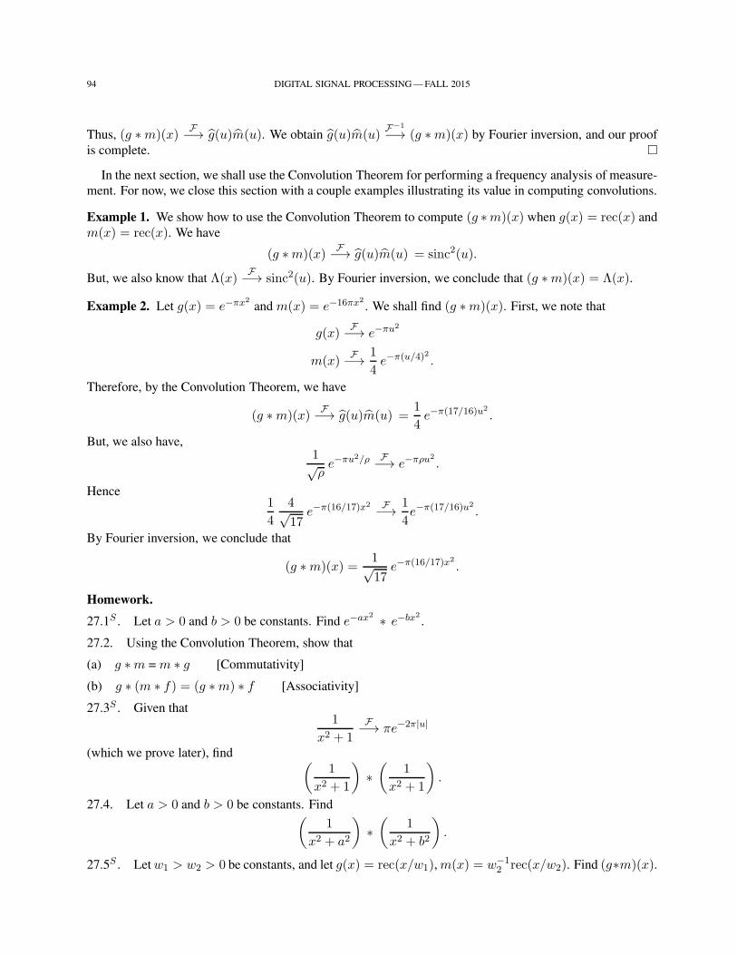
94 DIGITAL SIGNAL PROCESSING — FALL 2015
Thus, (g ∗m)(x)F−→ g(u)m(u). We obtain g(u)m(u)
F−1
−→ (g ∗m)(x) by Fourier inversion, and our proof
is complete.
In the next section, we shall use the Convolution Theorem for performing a frequency analysis of measure-
ment. For now, we close this section with a couple examples illustrating its value in computing convolutions.
Example 1. We show how to use the Convolution Theorem to compute (g ∗m)(x) when g(x) = rec(x) and
m(x) = rec(x). We have
(g ∗m)(x)F−→ g(u)m(u) = sinc2(u).
But, we also know that Λ(x)F−→ sinc2(u). By Fourier inversion, we conclude that (g ∗m)(x) = Λ(x).
Example 2. Let g(x) = e−πx2and m(x) = e−16πx2
. We shall find (g ∗m)(x). First, we note that
g(x)F−→ e−πu2
m(x)F−→ 1
4e−π(u/4)2 .
Therefore, by the Convolution Theorem, we have
(g ∗m)(x)F−→ g(u)m(u) =
1
4e−π(17/16)u2
.
But, we also have,1√ρe−πu2/ρ F−→ e−πρu2
.
Hence1
4
4√17
e−π(16/17)x2 F−→ 1
4e−π(17/16)u2
.
By Fourier inversion, we conclude that
(g ∗m)(x) =1√17
e−π(16/17)x2.
Homework.
27.1S . Let a > 0 and b > 0 be constants. Find e−ax2 ∗ e−bx2.
27.2. Using the Convolution Theorem, show that
(a) g ∗m = m ∗ g [Commutativity]
(b) g ∗ (m ∗ f) = (g ∗m) ∗ f [Associativity]
27.3S . Given that1
x2 + 1
F−→ πe−2π|u|
(which we prove later), find (1
x2 + 1
)∗(
1
x2 + 1
).
27.4. Let a > 0 and b > 0 be constants. Find(1
x2 + a2
)∗(
1
x2 + b2
).
27.5S . Let w1 > w2 > 0 be constants, and let g(x) = rec(x/w1), m(x) = w−12 rec(x/w2). Find (g∗m)(x).
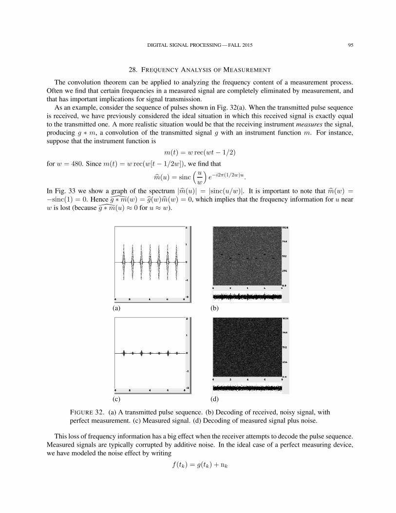
DIGITAL SIGNAL PROCESSING — FALL 2015 95
28. FREQUENCY ANALYSIS OF MEASUREMENT
The convolution theorem can be applied to analyzing the frequency content of a measurement process.
Often we find that certain frequencies in a measured signal are completely eliminated by measurement, and
that has important implications for signal transmission.
As an example, consider the sequence of pulses shown in Fig. 32(a). When the transmitted pulse sequence
is received, we have previously considered the ideal situation in which this received signal is exactly equal
to the transmitted one. A more realistic situation would be that the receiving instrument measures the signal,
producing g ∗ m, a convolution of the transmitted signal g with an instrument function m. For instance,
suppose that the instrument function is
m(t) = w rec(wt− 1/2)
for w = 480. Since m(t) = w rec(w[t− 1/2w]), we find that
m(u) = sinc( uw
)e−i2π(1/2w)u.
In Fig. 33 we show a graph of the spectrum |m(u)| = |sinc(u/w)|. It is important to note that m(w) =−sinc(1) = 0. Hence g ∗m(w) = g(w)m(w) = 0, which implies that the frequency information for u near
w is lost (because g ∗m(u) ≈ 0 for u ≈ w).
(a) (b)
(c) (d)
FIGURE 32. (a) A transmitted pulse sequence. (b) Decoding of received, noisy signal, with
perfect measurement. (c) Measured signal. (d) Decoding of measured signal plus noise.
This loss of frequency information has a big effect when the receiver attempts to decode the pulse sequence.
Measured signals are typically corrupted by additive noise. In the ideal case of a perfect measuring device,
we have modeled the noise effect by writing
f(tk) = g(tk) + nk
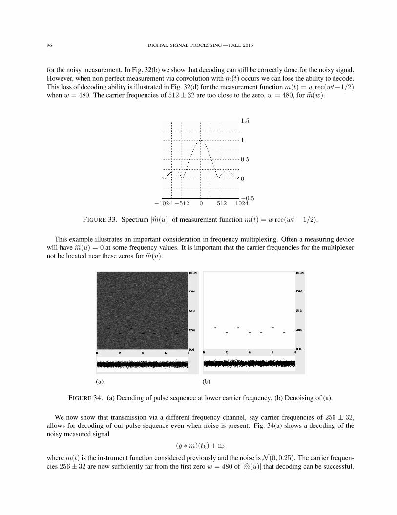
96 DIGITAL SIGNAL PROCESSING — FALL 2015
for the noisy measurement. In Fig. 32(b) we show that decoding can still be correctly done for the noisy signal.
However, when non-perfect measurement via convolution with m(t) occurs we can lose the ability to decode.
This loss of decoding ability is illustrated in Fig. 32(d) for the measurement function m(t) = w rec(wt−1/2)when w = 480. The carrier frequencies of 512± 32 are too close to the zero, w = 480, for m(w).
−1024 −512 0 512 1024−0.5
0
0.5
1
1.5
FIGURE 33. Spectrum |m(u)| of measurement function m(t) = w rec(wt− 1/2).
This example illustrates an important consideration in frequency multiplexing. Often a measuring device
will have m(u) = 0 at some frequency values. It is important that the carrier frequencies for the multiplexer
not be located near these zeros for m(u).
(a) (b)
FIGURE 34. (a) Decoding of pulse sequence at lower carrier frequency. (b) Denoising of (a).
We now show that transmission via a different frequency channel, say carrier frequencies of 256 ± 32,
allows for decoding of our pulse sequence even when noise is present. Fig. 34(a) shows a decoding of the
noisy measured signal
(g ∗m)(tk) + nk
where m(t) is the instrument function considered previously and the noise is N (0, 0.25). The carrier frequen-
cies 256± 32 are now sufficiently far from the first zero w = 480 of |m(u)| that decoding can be successful.
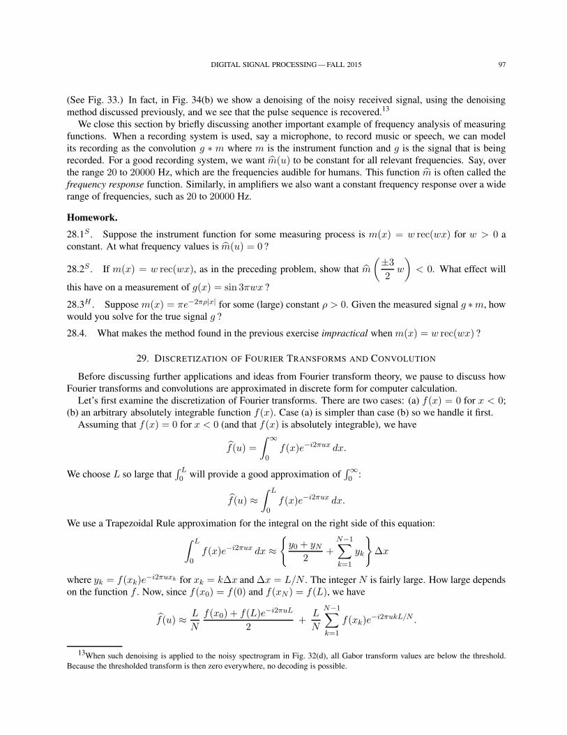
DIGITAL SIGNAL PROCESSING — FALL 2015 97
(See Fig. 33.) In fact, in Fig. 34(b) we show a denoising of the noisy received signal, using the denoising
method discussed previously, and we see that the pulse sequence is recovered.13
We close this section by briefly discussing another important example of frequency analysis of measuring
functions. When a recording system is used, say a microphone, to record music or speech, we can model
its recording as the convolution g ∗ m where m is the instrument function and g is the signal that is being
recorded. For a good recording system, we want m(u) to be constant for all relevant frequencies. Say, over
the range 20 to 20000 Hz, which are the frequencies audible for humans. This function m is often called the
frequency response function. Similarly, in amplifiers we also want a constant frequency response over a wide
range of frequencies, such as 20 to 20000 Hz.
Homework.
28.1S . Suppose the instrument function for some measuring process is m(x) = w rec(wx) for w > 0 a
constant. At what frequency values is m(u) = 0 ?
28.2S . If m(x) = w rec(wx), as in the preceding problem, show that m
(±3
2w
)< 0. What effect will
this have on a measurement of g(x) = sin 3πwx ?
28.3H . Suppose m(x) = πe−2πρ|x| for some (large) constant ρ > 0. Given the measured signal g ∗m, how
would you solve for the true signal g ?
28.4. What makes the method found in the previous exercise impractical when m(x) = w rec(wx) ?
29. DISCRETIZATION OF FOURIER TRANSFORMS AND CONVOLUTION
Before discussing further applications and ideas from Fourier transform theory, we pause to discuss how
Fourier transforms and convolutions are approximated in discrete form for computer calculation.
Let’s first examine the discretization of Fourier transforms. There are two cases: (a) f(x) = 0 for x < 0;
(b) an arbitrary absolutely integrable function f(x). Case (a) is simpler than case (b) so we handle it first.
Assuming that f(x) = 0 for x < 0 (and that f(x) is absolutely integrable), we have
f(u) =
∫ ∞
0f(x)e−i2πux dx.
We choose L so large that∫ L0 will provide a good approximation of
∫∞0 :
f(u) ≈∫ L
0f(x)e−i2πux dx.
We use a Trapezoidal Rule approximation for the integral on the right side of this equation:
∫ L
0f(x)e−i2πux dx ≈
y0 + yN
2+
N−1∑
k=1
yk
∆x
where yk = f(xk)e−i2πuxk for xk = k∆x and ∆x = L/N . The integer N is fairly large. How large depends
on the function f . Now, since f(x0) = f(0) and f(xN ) = f(L), we have
f(u) ≈ L
N
f(x0) + f(L)e−i2πuL
2+
L
N
N−1∑
k=1
f(xk)e−i2πukL/N .
13When such denoising is applied to the noisy spectrogram in Fig. 32(d), all Gabor transform values are below the threshold.
Because the thresholded transform is then zero everywhere, no decoding is possible.
98 DIGITAL SIGNAL PROCESSING — FALL 2015
Based on this last approximation, the computer is used to compute discrete approximations of f(mL
),
via
f(mL
)≈ L
N
N−1∑
k=0
gke−i2πmk/N (51)
with g0 = [f(0) + f(L)]/2, and gk = f(xk) for k = 1, 2, . . . , N − 1. Hence, FAWAV computes L/Ntimes an N -point FFT, in order to approximate these transform values. In FAWAV, Equation (51) is typi-
cally applied for m = −N/2, . . . , 0, . . . , N/2, which corresponds to the option [0,L] → [-A,A] in the
Transform/Fourier procedure.
We now turn to the general case (b) of an arbitrary, absolutely integrable function f(x). Here we choose
L so large that∫∞−∞ is well-approximated by
∫ L/2−L/2:
f(u) =
∫ ∞
−∞f(x)e−i2πux dx
≈∫ L/2
−L/2f(x)e−i2πux dx.
Again, we use a trapezoidal rule approximation for the definite integral
∫ L/2
−L/2f(x)e−i2πux dx ≈ L
N
Y0 + YN
2+
N−1∑
k=1
Yk
(52)
where Yk = f(xk)e−i2πuxk and xk = −L/2+ k∆x for k = 0, 1, . . . , N and ∆x = L/N . For u = m/L, we
get
Yk = f(xk)e−i2π(m/L)[−L/2+kL/N ]
= f(xk)eiπme−i2πmk/N
= f(xk)(−1)m e−i2πmk/N .
We have the special cases
Y0 = f(x0)(−1)m = f(−L/2)(−1)m, and YN = f(xN )(−1)m e−i2πm = f(L/2)(−1)m.
Substituting our formulas back into (52) we get
f(mL
)≈ (−1)m
L
N
N−1∑
k=0
gke−i2πmk/N
where g0 =[f(−L/2)+f(L/2)
]/2, and gk = f(xk) for k = 1, . . . , N−1. Thus, we can again approximate
the transform values f(m/L) by computing an FFT, along with multiplication by factors (−1)mL/N .
These approximate calculations of Fourier transforms work reasonably well with regular functions, as the
following two examples show.
Example 1. Let f(x) = e−πx2. Using FAWAV, we approximate the Fourier transform over [−16, 16] with
1024 points. Computing e−πx2(the Fourier transform as a function of x) over [−16, 16] as well, we find that
the sup-norm difference between the exact transform and the FAWAV computed approximation is 2.89×10⁻¹⁵ .
Thus, (52) provides an excellent approximation.
DIGITAL SIGNAL PROCESSING — FALL 2015 99
Example 2. Let f(x) = e−2π|x|. We again approximate a Fourier transform over [−16, 16] using 1024points. The sup-norm difference between the exact transform [(1/π)/(x2 + 1) as a function of x] and the
FAWAV approximation is 1.8 × 10⁻³, so FAWAV provides a reasonable graphical approximation. If we use
N = 4096 points instead, then the sup-norm error decreases to 1.1× 10⁻⁴.
Discrete approximation of convolution. We conclude by briefly describing the discrete approximation of
convolution. Since f · g F−1
−→ f ∗g, we obtain a discrete approximation to convolution by replacing the Fourier
transforms f and g by FFT approximations Fn and Gn, respectively, and then applying the inverse FFT
to the product FnGn of those FFTs. Thus, we obtain the following discrete approximation for convolution:
(f ∗ g)(xk) ≈ F−1FnGn.
Example 3. We graph rec(x), and rec(x) again, on the interval [−4, 4] using 1024 points. Using the con-
volution procedure of FAWAV, we obtain a numerical approximation of rec ∗ rec. The sup-norm difference
between this numerical approximation and the exact convolution Λ(x) = (1 − |x|)(|x| ≤ 1) is 3.9 × 10⁻³.
We have obtained a reasonable graphical approximation. If we use 4096 points the sup-norm decreases to
9.8× 10⁻⁴.
Example 4. Previously we found that e−πx2 ∗ e−16πx2=
1√17
e−π(16/17)x2. The sup-norm difference
between this exact convolution and the FAWAV approximation on the interval [−8, 8] is 9.27 × 10⁻¹⁵. The
approximation is excellent.
Homework.
29.1. Find the sup-norm difference between the exact convolution e−πx2 ∗ e−πx2and its FAWAV computed
approximation over the interval [−8, 8] using 1024 points.
29.2S . Find the sup-norm difference between the exact convolution (x2+1)−1 ∗ (x2+1)−1 and its FAWAV
computed approximation over the interval [−8, 8] using 1024 points.
29.3S . Find a formula for the Fourier transform of the correlation
f(x) =
∫ ∞
−∞g(t)m(t− x) dt
of g with m. How would this correlation be approximated using FFTs?
30. INVERSION OF FOURIER TRANSFORMS [OPTIONAL]
In this optional section we shall prove a couple of theorems which justify the Fourier inversion formula
derived previously. We shall study the validity of the formula
limL→∞
∫ L
−Lf(u)ei2πux du = f(x). (53)
To prove (53) we need a couple of lemmas, both of which are interesting in their own right.
Lemma 1 [Riemann-Lebesgue Lemma]. Suppose that g(x) satisfies∫∞−∞ |g(x)| dx < ∞. Then
g(L) → 0 and g(−L) → 0 when L → ∞.
100 DIGITAL SIGNAL PROCESSING — FALL 2015
Proof. First, consider a step function
g(x) =
M∑
k=1
ak [bk ≤ x ≤ ck]
=
M∑
k=1
ak rec
(x−mk
wk
)
where mk =ck + bk
2and wk =
ck − bk2
. We then have
g(u) =M∑
k=1
akwk sinc(wku)e−i2πmku.
Hence
g(L) =M∑
k=1
akwksinπwkL
πwkLe−i2πmkL.
Because L is in the denominator of each term, we conclude that g(L) → 0 as L → ∞. Similarly, we also
have g(−L) → 0 as L → ∞. Thus, the theorem holds for every step function.
Second, consider an arbitrary function g(x) for which∫∞−∞ |g(x)| dx < ∞. It is proved in courses of
mathematical analysis that, for any given ǫ > 0, we can find a step function gǫ such that14
∫ ∞
−∞|g(x)− gǫ(x)| dx < ǫ. (54)
But then
|g(L)| =∣∣∣ (g − gǫ)(L) + gǫ(L)
∣∣∣
≤∣∣∣ (g − gǫ)(L)
∣∣∣+ |gǫ(L)|
=
∣∣∣∣∫ ∞
−∞[g(x)− gǫ(x)]e
−i2πLx dx
∣∣∣∣+ |gǫ(L)|
≤∫ ∞
−∞|g(x)− gǫ(x)| dx+ |gǫ(L)|
< ǫ+ |gǫ(L)| .
Since gǫ is a step function, we know that gǫ(L) → 0 as L → ∞. So, we may choose L large enough that
|gǫ(L)| < ǫ. Hence,
|g(L)| < 2ǫ
for all sufficiently large L. Therefore, g(L) → 0 as L → ∞. Similar reasoning shows that g(−L) → 0 as
L → ∞.
14It is easy to see that (54) holds for g piecewise continuous: just divide a large interval [−L, L] into small enough subintervals
and define gǫ to be equal to g at each left endpoint of each subinterval and 0 outside of [−L,L].
DIGITAL SIGNAL PROCESSING — FALL 2015 101
Lemma 2. Suppose that∫∞−∞ |g(x)| dx < ∞ and
∫∞−∞ |x g(x)| dx < ∞. Then
x g(x)F−→ i
2π
dg
du.
Proof. By differentiating under the integral sign, we obtain
dg
du=
d
du
∫ ∞
−∞g(x)e−i2πux dx
=
∫ ∞
−∞
∂
∂u
[g(x)e−i2πux
]dx.
(55)
[That (55) holds is proved in Fourier Analysis, Section 6.3.] But, we also have
∂
∂u
[g(x)e−i2πux
]= −i2πx g(x)e−i2πux.
Hence
i
2π
dg
du=
i
2π(−i2π)
∫ ∞
−∞x g(x)e−i2πux dx
= F [x g(x)](u)
and that completes the proof.
Remark. Lemma 2 is useful in its own right. For example, it can be used to derive the following two Fourier
transforms:
(a) x e−πx2 F−→ − iu e−πu2
(b) x e−2π|x| F−→ −i
π2
u
(u2 + 1)2.
We are now ready to prove the following Fourier transform inversion theorem.
Theorem 1. Suppose that∫∞−∞ |f(x)| dx < ∞ and that f ′(x0+) and f ′(x0−) are finite. Then, if f is
continuous at x0, we have
limL→∞
∫ L
−Lf(u)ei2πux du = f(x0).
Or, if f has a jump discontinuity at x0, then
limL→∞
∫ L
−Lf(u)ei2πux du =
1
2[f(x0+) + f(x0−)] .
Proof. The complete proof can be found in Fourier Analysis, Section 6.5. Here we will only discuss the case
of x0 being a point of continuity for f , since this is the more important case and we can provide a simpler
proof than the one given in Fourier Analysis.
We shall use the notation SL(x) =
∫ L
−Lf(u)ei2πux du introduced earlier. With this notation, we need
to prove that SL(x0) → f(x0) as L → ∞. First, we may reduce to the case x0 = 0. Why? Because
f(u)ei2πux0 = f(x+ x0)(u), hence for g(x) = f(x+ x0) we have
SL(x0) =
∫ L
−Lg(u)ei2πu 0 du
102 DIGITAL SIGNAL PROCESSING — FALL 2015
and g′(0+) = f ′(x0+), g′(0−) = f ′(x0−), g(0) = f(x0). Therefore, by proving that
limL→∞
∫ L
−Lg(u)ei2πu 0 du = g(0)
we obtain
limL→∞
∫ L
−Lf(u)ei2πux0 du = f(x0).
Thus, without loss of generality, we shall assume that x0 = 0.
Second, we may assume that f(0) = 0. Why? We have
limL→∞
∫ L
−Lce−πu2
du =
∫ ∞
−∞ce−πu2
du = c,
so inversion works at x0 = 0 for all functions of the form ce−πx2. Let g(x) = f(x) − f(0)e−πx2
. Then,
g(0) = 0 and g′(0+) = f ′(0+), g′(0−) = f ′(0−). If we prove inversion for g(x), then inversion will also
work for f(x) = g(x) + f(0)e−πx2. Therefore, without loss of generality, we shall assume that f(0) = 0.
We now prove that limL→∞
SL(0) = 0, which will complete our proof. Consider the auxiliary function
g(x) = f(x)/x. Because f ′(0+) and f ′(0−) are finite, it follows that g(x) is bounded for x near 0. Therefore∫∞−∞ |g(x)| dx < ∞. The Riemann-Lebesgue Lemma then tells us that
g(L) → 0 and g(−L) → 0 as L → ∞.
But, f(x) = x g(x), hence Lemma 2 tells us that
f(u) =i
2π
dg
du.
We thus obtain
SL(0) =
∫ L
−Lf(u) du
=
∫ L
−L
i
2π
dg
dudu
=i
2π[g(L)− g(−L)]
→ 0 as L → ∞,
and that completes our proof.
There is a second inversion theorem for Fourier transforms, which is somewhat analogous to the uniform
convergence theorem for Fourier series.
Theorem 2. If f is continuous and∫∞−∞ |f(x)| dx < ∞, and
∫∞−∞ |f(u)| du < ∞, then
f(x) =
∫ ∞
−∞f(u)ei2πux du
holds for all x-values.
Proof. The complete proof can be found in Fourier Analysis, Section 6.4. Here we will just provide a rough
sketch of this proof. We may assume, without loss of generality, that x0 = 0 [for the same reasons as in
DIGITAL SIGNAL PROCESSING — FALL 2015 103
the proof of Theorem 1.] We then need to show that f(0) =∫∞−∞ f(u) du. Let C stand for the constant∫∞
−∞ f(u) du. We have
C =
∫ ∞
−∞f(u) 1 du
= limρ→0+
∫ ∞
−∞f(u)e−πρ2u2
du.
But, we also have,∫ ∞
−∞f(u)e−πρ2u2
du =
∫ ∞
−∞
(∫ ∞
−∞f(x)e−i2πux dx
)e−πρ2u2
du
=
∫ ∞
−∞f(x)
(∫ ∞
−∞e−πρ2u2
e−i2πux du
)dx
=
∫ ∞
−∞f(x)
1
ρe−πx2/ρ2 dx
−−−−→ρ→0+
∫ ∞
−∞f(x)δ(x) dx = f(0).
From these last two sets of calculations, we conclude that C = f(0), and we are done.
Homework.
30.1. Show that formulas (a) and (b) hold in the Remark on p. 101.
30.2. Show that ∫ ∞
−∞
1
π
1
u2 + 1ei2πux dx = e−2π|x|
and use this result to prove that1
x2 + 1
F−→ πe−2π|u|.
In Problems 30.3–30.6 we outline the remainder of the proof of Theorem 1, p. 101.
30.3S . Define the function I(α), for α ≥ 0 by
I(α) =
∫ ∞
0e−αu sin 2πu
πudu.
Prove that
I(0) =
∫ ∞
−∞sincu eiπu du
= limL→∞
∫ L
−Lsincu ei2πu(1/2) du.
30.4S . Compute I ′(α) and use this to find I(α) for α > 0 [given that I(α) → 0 as α → ∞], and then show
that
I(0) =1
2=
1
2
[rec
(1
2+
)+ rec
(1
2−)]
[Thus proving the inversion theorem for rec(x) at x = 1/2.]
104 DIGITAL SIGNAL PROCESSING — FALL 2015
30.5S . For x0 a point of jump discontinuity in the statement of Theorem 1 on p. 101, let g(x) be defined by
g(x) = f(x) + C rec(x− x0 + 1/2)
where C = f(x0+)− f(x0−). Use g and the result of Problem 30.4 to prove that
limL→∞
∫ L
−Lf(u)ei2πux du =
1
2
[f(x0+) + f(x0−)
].
Thus completing the proof of Theorem 1.
31. SAMPLING THEORY
Sampling theory—the reconstruction of signals from discrete values of those signals—plays a fundamental
role in communications. For example, it is used in building CD music players and in transmitting multiple
telephone messages. The signals that can be reconstructed from evenly-spaced discrete values are called
“band-limited.”
Definition. A function f(x) is called band-limited, if f(u) = 0 for |u| ≥ L, where L is some finite positive
number.
The following theorem, which has been credited to Shannon, and to Nyquist, as well as Whittaker, is the
fundamental theorem in sampling theory. It gives a precise formula for reconstructing a band-limited function.
Theorem. Suppose that f(x) is continuous and absolutely integrable, and f(x) is band-limited. The signal
f(x) can be reconstructed for all x-values using the sequence of discrete valuesf( n
2L
)∞
n=−∞. The
reconstruction formula is
f(x) =
∞∑
n=−∞f( n
2L
)sinc(2Lx− n). (56)
Proof. By Fourier inversion,
f(x) =
∫ L
−Lf(u)ei2πux du.
Hence
1
2Lf( n
2L
)=
1
2L
∫ L
−Lf(u)ei2πnu/2L du.
This last integral is the (−n)th Fourier coefficient for f(u), restricted to the interval [−L,L], and expanded
in a 2L-period Fourier series. Define fL by fL(u) = f(u) on [−L,L), and fL(u+2L) = fL(u). That is, fL
has period 2L and equals f on the interval [−L,L). Using
1
2Lf
(−n
2L
)as Fourier coefficients, we have
fL(u) =
∞∑
n=−∞
1
2Lf
(−n
2L
)ei2πnu/2L. (57)
Multiplying (57) by
W (u) =
1 if |u| ≤ L
0 if |u| > L
DIGITAL SIGNAL PROCESSING — FALL 2015 105
and combining with Fourier inversion, we obtain
f(x) =
∫ L
−Lf(u)ei2πux du
=
∫ L
−LfL(u)W (u)ei2πux du
=
∫ L
−L
[ ∞∑
n=−∞
1
2Lf
(−n
2L
)W (u)ei2πnu/2L
]ei2πux du
=
∞∑
n=−∞f
(−n
2L
)1
2L
∫ L
−LW (u)ei2πu(x+n/2L) du.
We also have
1
2L
∫ L
−LW (u)ei2πux du =
∫ ∞
−∞
1
2Lrec( u
2L
)ei2πux du
=1
2L2L sinc(2Lx)
= sinc(2Lx).
Therefore, combining these last two sets of calculations, we obtain
f(x) =
∞∑
n=−∞f
(−n
2L
)sinc
[2L(x+
n
2L
)]
=
∞∑
n=−∞f
(−n
2L
)sinc(2Lx+ n)
=−∞∑
m=∞f(m
2L
)sinc(2Lx−m)
=∞∑
n=−∞f( n
2L
)sinc(2Lx− n)
and that completes our proof.
Remark. The last equality above may seem a bit mysterious. As with Fourier series, we shall assume that
the reconstruction series in sampling theory is defined as a limit of partial sums:
∞∑
n=−∞f( n
2L
)sinc(2Lx− n) = lim
N→∞
N∑
n=−N
f( n
2L
)sinc(2Lx− n).
106 DIGITAL SIGNAL PROCESSING — FALL 2015
Hence the last equality in the proof is shorthand for the following calculation:
−∞∑
m=∞f(m
2L
)sinc(2Lx−m) = lim
N→∞
−N∑
m=N
f(m
2L
)sinc(2Lx−m)
= limN→∞
N∑
n=−N
f( n
2L
)sinc(2Lx− n)
=
∞∑
n=−∞f( n
2L
)sinc(2Lx− n).
Example. Consider the function f(x) = sinc2(4x − 3) + sinc2(8x − 2). We shall show that this function
is band-limited and obtain a reconstruction series for it. By the shifting and scaling properties of the Fourier
transform, we find that
sinc2(4x− 3) = sinc2[4(x− 3/4)]F−→ sinc2(4x)(u)e−i2π(3/4)u
=1
4Λ(u4
)e−i3πu/2.
Similarly,
sinc2(8x− 2)F−→ 1
8Λ(u8
)e−iπu/2.
Hence, by linearity of the Fourier transform,
f(u) =1
4Λ(u4
)e−i3πu/2 +
1
8Λ(u8
)e−iπu/2.
We conclude that f(u) = 0 for |u| ≥ 8. Therefore, f is band-limited. It can be reconstructed from its discrete
samplesf( n
16
)as follows
f(x) =
∞∑
n=−∞f( n
16
)sinc(16x− n).
Application 1 [Time-multiplexing]. An important application of the sampling theorem, in electronic com-
munication, is the sending of multiple messages over a single transmission channel. For example, around 104
telephone messages can be sent over one fiber optic cable; and an even greater number of cell-phone mes-
sages can be transmitted via one microwave transmission over a satellite link. This latter example illustrates
how millions of cell-phone messages can be transmitted simultaneously via a relatively small size satellite
network around the earth. The basic method of the time-multiplexing technique consists of the following
three steps:
Step 1. For any given message g, pass the transmission through a low-pass filter which only retains fre-
quencies in the message that lie below the magnitude L. This filtered message f satisfies f(u) =g(u)W (u) where W is a function that is zero for |u| ≥ L. For telephone transmissions, the value
of L is typically 4000 Hz. This “muddies” the sound somewhat, which is why it often takes people
a few calls to recognize an acquaintance on the phone, although their words are clear enough to be
understandable.
DIGITAL SIGNAL PROCESSING — FALL 2015 107
Step 2. Sample values of the low-pass filtered messagef( n
2L
)are generated and approximated by finite
bit-length (floating point) approximationsfd
( n
2L
). Those finite bit-sequences are then transmit-
ted with time-delays of1
2Lbetween them. Because of these time-delays, multiple signals can be
interleaved within the gaps.
Step 3. At the receiving end, an approximation of g(x) is created as follows:
g(x) ≈N∑
n=−N
fd
( n
2L
)sinc(2Lx− n) (58)
where N is a (large) finite positive integer.
As the success of long-distance telephony and cellular communication testifies, (58) provides a serviceable
approximation to human voices.
Application 2 [CD recording]. Recordings of CD music make use of the sampling theorem. The basic
mathematics is similar to that discussed for Application 1, but here the value of L is typically 22050 Hz (an
upper range for human hearing). In this case, the sampling rate of 2L samples/sec is 44100 samples/sec
(frequently given as 44100 Hz, where here Hz stands for samples/sec rather than cycles/sec). The division
of the amplitudes into bit-sequences, the approximation of values of f by fd, is also much finer than for
telephony: 16-bits or 32-bits are used for floating point approximations in CD recording, while only 8-bits
are used for telephony (to allow more room for simultaneous transmissions). The bits 0 and 1 are encoded
on the CD disc by the use of pits in the CD surface. The presence of a pit disrupts the reflection back to a
detector of a laser beam shined on the disc, while the absence of a pit allows for undisrupted reflection back to
the detector. When the detector gives a low response, that signals the bit 0, and when it gives a high response
that signals the bit 1.
Homework.
31.1S . Find the smallest value of L so that f(u) = 0 for |u| ≥ L, given that f(x) = sinc2(4x− 3).
31.2S . Write out the sampling series reconstruction for f(x) = sinc2(4x−3) using the value of L from the
previous exercise.
31.3. Find the smallest value of L so that f(u) = 0 for |u| ≥ L, given that f(x) = 4 sinc2(16x − 5) +2 sinc2(32x− 7).
31.4. Write out the sampling series reconstruction for f(x) = 4 sinc2(16x − 5) + 2 sinc2(32x − 7) using
the value of L from the previous exercise.
32. NYQUIST RATE, NYQUIST SERIES
If f is band-limited, then for some L we have f(u) = 0 when |u| ≥ L. The smallest possible such value
of L is called the Nyquist frequency LN
.
Example 1. For f(x) = sinc2(8x − 5), we shall find the Nyquist frequency. First, note that f(x) =sinc2[8(x − 5/8)]. Hence, by the scaling and shifting properties, we obtain
sinc2[8(x− 5/8)]F−→ sinc2(8x)(u) e−i2π(5/8)u
=1
8Λ(u8
)e−i2π(5/8)u.
108 DIGITAL SIGNAL PROCESSING — FALL 2015
Since e−i2π(5/8)u never equals 0, it follows that f(u) = 0 precisely when Λ(u/8) = 0. That is, when
|u/8| ≥ 1. Thus, f(u) = 0 when |u| ≥ 8. Hence the Nyquist frequency is LN
= 8.
When the Nyquist frequency LN
is used in the sampling series to reconstruct f(x), we call that series the
Nyquist series. The value 2LN
, which has units of samples/time-unit (typically samples/sec) is called the
Nyquist rate (or Nyquist sampling rate).
Example 2. For f(x) = sinc2(8x − 5) we found in Example 1 that the Nyquist frequency is LN
= 8. Thus
the Nyquist series for reconstructing f(x) is
f(x) =
∞∑
n=−∞f( n
16
)sinc(16x − n).
We can approximate f(x) by a partial sum:
f(x) ≈ SM (x) =
M∑
n=−M
f( n
16
)sinc(16x − n).
Using an x-interval of [−2, 2] and 1024 points, we obtain the following sup-norm errors for this approxima-
tion:M ‖f − SM‖sup16 8.57 × 10⁻³
32 3.39 × 10⁻⁴
64 1.03 × 10⁻⁵
With M = 32, we are getting a reasonably close approximation using only the dataf( n
16
)32
n=−32, which
leaves gaps of length 1/16 between successive data values. These gaps are where other signal data can be
interleaved for multiple transmissions.
Homework.
32.1S . Find the Nyquist series for f(x) = 3 sinc2(4x−2). Plot f(x) and SM for M = 16, 32, and 64, over
the interval [−2, 2]. Find the sup-norm differences ‖f − SM‖ for those values of M .
32.2. Find the Nyquist series for f(x) = 2 sinc2(4x−2)−4 sinc2(8x−1). Plot f(x) and SM for M = 16,
32, and 64, over the interval [−2, 2]. Find the sup-norm differences ‖f − SM‖ for those values of M .
33. OVERSAMPLING
Suppose that f is bandlimited with f(u) = 0 for |u| ≥ LN
, its Nyquist frequency. Frequently in applica-
tions, such as CD music, the sampling rate is taken as a multiple of the Nyquist rate 2LN
. In 2×-oversampling,
which we consider here, the rate used is 4LN
.
To see why a rate of 4LN
, rather than the minimal 2LN
, is used we need to reconsider the proof of the
sampling theorem. Instead of expanding f(u) in a 2LN
-period Fourier series, we expand it in a 4LN
-period
Fourier series:
fL(u) =
∞∑
n=−∞
1
4LN
f
( −n
4LN
)ei2π(n/4LN )u.
We then multiply both sides of this equation by the function
W (u) =
1 if |u| ≤ LN
2− |u|/LN
if LN
< |u| < 2LN
0 if |u| ≥ 2LN
DIGITAL SIGNAL PROCESSING — FALL 2015 109
and, using fL(u)W (u) = f(u), obtain
f(u) =∞∑
n=−∞
1
4LN
f
( −n
4LN
)W (u)ei2π(n/4LN )u.
We now multiply this equation by ei2πux and perform Fourier inversion. Using the fact that f(u) = 0 for
|u| ≥ 2LN
), we have
f(x) =
∫ 2LN
−2LN
f(u)ei2πux du
=
∞∑
n=−∞
1
4LN
f
( −n
4LN
)∫ 2LN
−2LN
W (u)ei2πu(x+n/4LN
) du.
(59)
We will now establish the following formula:
1
4LN
∫ 2LN
−2LN
W (u)ei2πux du =3
4sinc(3L
Nx) sinc(L
Nx). (60)
To establish (60), we shall use L in place of LN
(in order to keep the notation simpler). Because W is an even
function, we have
1
4L
∫ 2L
−2LW (u)ei2πux du =
1
2L
∫ 2L
0W (u) cos 2πux du
=1
2L
∫ L
01 cos 2πux du+
1
2L
∫ 2L
L
(2− u
L
)cos 2πux du.
The first integral on the right of the last equation is
1
2L
∫ L
01 cos 2πux du =
sin 2πux
2L · 2πx
∣∣∣∣u=L
u=0
=sin 2πLx
2L · 2πx .
The second integral on the right requires integration by parts. The integration by parts rule can be written as
∫w dv = wv −
∫v dw.
Using w =1
2L
(2− u
L
)and dv = cos 2πux du, we obtain
110 DIGITAL SIGNAL PROCESSING — FALL 2015
1
2L
∫ 2L
L
(2− u
L
)cos 2πux du
=1
2L
(2− u
L
) sin 2πux
2πx
∣∣∣∣u=2L
u=L
+1
2L2
∫ 2L
L
sin 2πux
2πxdu
=− sin 2πLx
2L · 2πx − cos 2πux
2L2(2πx)2
∣∣∣∣u=2L
u=L
=− sin 2πLx
2L · 2πx +cos 2πLx− cos 4πLx
2L2(2πx)2.
Combining these two integral calculations, we then have
1
4L
∫ 2L
−2LW (u)ei2πux du =
cos 2πLx− cos 4πLx
2L2(2πx)2.
The only thing that remains is to show that
cos 2πLx− cos 4πLx
2L2(2πx)2=
3
4sinc(3Lx) sinc(Lx).
To see this, we make use of the following trigonometric identity:
cos(φ− θ)− cos(φ+ θ) = 2 sinφ sin θ.
Using φ = 3πLx and θ = πLx, this identity becomes
cos 2πLx− cos 4πLx = 2 sin 3πLx sinπLx.
Therefore, we have
cos 2πLx− cos 4πLx
2L2(2πx)2=
2 sin 3πLx sinπLx
2L2(2πx)2
=3
4
sin 3πLx
3πLx
sinπLx
πLx
=3
4sinc(3Lx) sinc(Lx).
DIGITAL SIGNAL PROCESSING — FALL 2015 111
Using L = LN
, we have
1
4LN
∫ 2LN
−2LN
W (u)ei2πux du =3
4sinc(3L
Nx) sinc(L
Nx)
which is the same as (60).
Substituting (60) into (59), we obtain
f(x) =
∞∑
n=−∞f
( −n
4LN
)S
(x+
n
4LN
)
where
S(x) =3
4sinc(3L
Nx) sinc(L
Nx).
Hence, by substituting m = −n, we obtain our 2×-oversampled reconstruction formula for f(x):
f(x) =
∞∑
m=−∞f
(m
4LN
)S
(x− m
4LN
)
where (61)
S(x) =3
4sinc(3L
Nx) sinc(L
Nx).
The kernel function S(x) we shall refer to as the double-sinc function.
Formula (61) is important when finite-time delay effects are considered in sampling. We have to consider
such effects when only a finite number of samples (within ±τ of the time x) are used to reconstruct f(x). For
example, if Nyquist sampling is used, we examine the partial sum approximation
f(x) ≈ S1τ (x) =
M∑
n=−M
f
(n
2LN
)sinc(2L
Nx− n)
(∣∣∣∣x− n
2LN
∣∣∣∣ ≤ τ
)
where M is the largest value allowed for the finite time-interval [−A,A] over which reconstruction occurs.
While with 2×-oversampling, we have two different partial sums that we examine
f(x) ≈ S2τ (x) =
2M∑
−2M
f
(n
4LN
)sinc(4L
Nx− n)
(∣∣∣∣x− n
4LN
∣∣∣∣ ≤ τ
)
and
f(x) ≈ S3τ (x) =
2M∑
−2M
f
(n
4LN
)S
(x− n
4LN
)(∣∣∣∣x− n
4LN
∣∣∣∣ ≤ τ
).
Example. Consider the function
f(x) = 2 sinc2(2x− 2) + 4 sinc2(3x− 12) − 2 sinc2(4x+ 12).
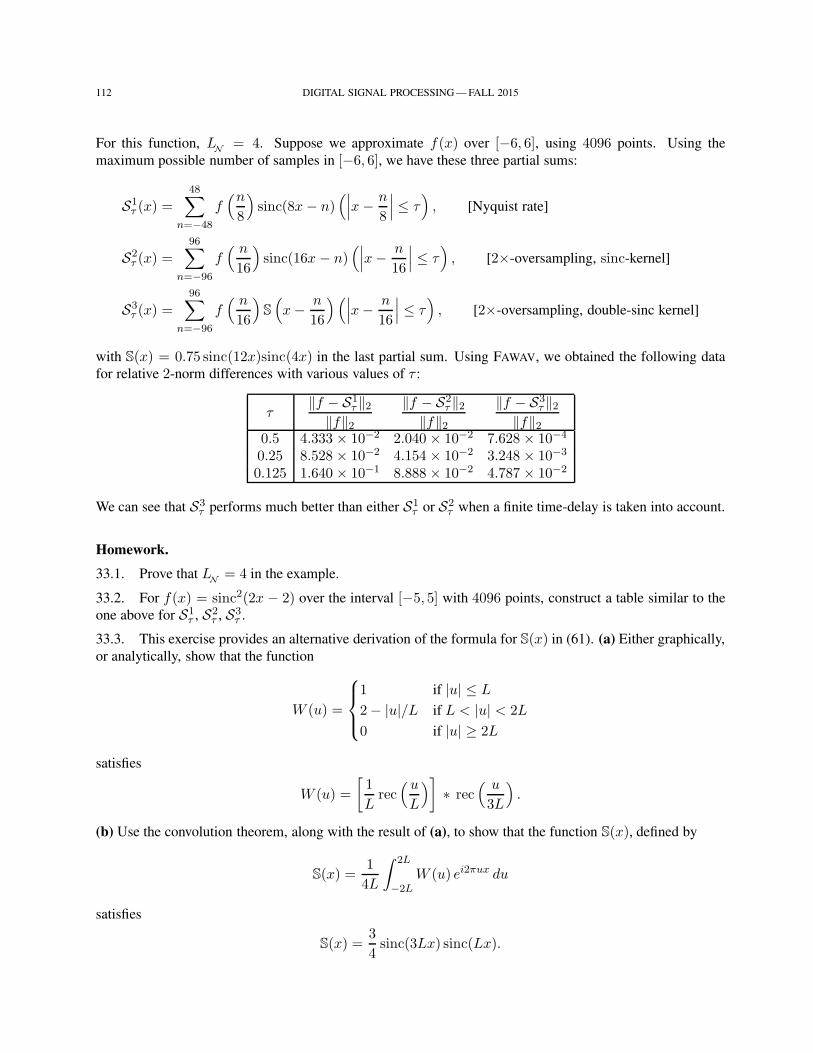
112 DIGITAL SIGNAL PROCESSING — FALL 2015
For this function, LN
= 4. Suppose we approximate f(x) over [−6, 6], using 4096 points. Using the
maximum possible number of samples in [−6, 6], we have these three partial sums:
S1τ (x) =
48∑
n=−48
f(n8
)sinc(8x− n)
(∣∣∣x− n
8
∣∣∣ ≤ τ), [Nyquist rate]
S2τ (x) =
96∑
n=−96
f( n
16
)sinc(16x − n)
(∣∣∣x− n
16
∣∣∣ ≤ τ), [2×-oversampling, sinc-kernel]
S3τ (x) =
96∑
n=−96
f( n
16
)S
(x− n
16
)(∣∣∣x− n
16
∣∣∣ ≤ τ), [2×-oversampling, double-sinc kernel]
with S(x) = 0.75 sinc(12x)sinc(4x) in the last partial sum. Using FAWAV, we obtained the following data
for relative 2-norm differences with various values of τ :
τ‖f − S1
τ ‖2‖f‖2
‖f − S2τ ‖2
‖f‖2‖f − S3
τ ‖2‖f‖2
0.5 4.333 × 10⁻² 2.040 × 10⁻² 7.628 × 10⁻⁴
0.25 8.528 × 10⁻² 4.154 × 10⁻² 3.248 × 10⁻³
0.125 1.640 × 10⁻¹ 8.888 × 10⁻² 4.787 × 10⁻²
We can see that S3τ performs much better than either S1
τ or S2τ when a finite time-delay is taken into account.
Homework.
33.1. Prove that LN
= 4 in the example.
33.2. For f(x) = sinc2(2x − 2) over the interval [−5, 5] with 4096 points, construct a table similar to the
one above for S1τ , S2
τ , S3τ .
33.3. This exercise provides an alternative derivation of the formula for S(x) in (61). (a) Either graphically,
or analytically, show that the function
W (u) =
1 if |u| ≤ L
2− |u|/L if L < |u| < 2L
0 if |u| ≥ 2L
satisfies
W (u) =
[1
Lrec(uL
)]∗ rec
( u
3L
).
(b) Use the convolution theorem, along with the result of (a), to show that the function S(x), defined by
S(x) =1
4L
∫ 2L
−2LW (u) ei2πux du
satisfies
S(x) =3
4sinc(3Lx) sinc(Lx).
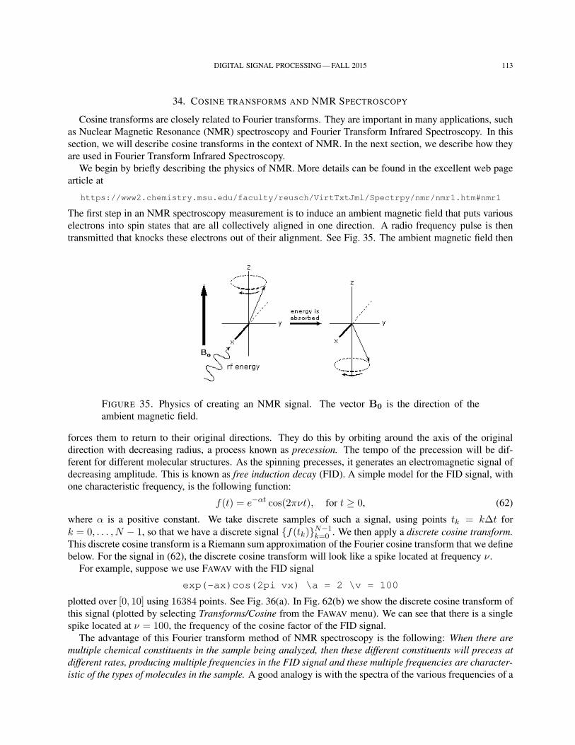
DIGITAL SIGNAL PROCESSING — FALL 2015 113
34. COSINE TRANSFORMS AND NMR SPECTROSCOPY
Cosine transforms are closely related to Fourier transforms. They are important in many applications, such
as Nuclear Magnetic Resonance (NMR) spectroscopy and Fourier Transform Infrared Spectroscopy. In this
section, we will describe cosine transforms in the context of NMR. In the next section, we describe how they
are used in Fourier Transform Infrared Spectroscopy.
We begin by briefly describing the physics of NMR. More details can be found in the excellent web page
article at
https://www2.chemistry.msu.edu/faculty/reusch/VirtTxtJml/Spectrpy/nmr/nmr1.htm#nmr1
The first step in an NMR spectroscopy measurement is to induce an ambient magnetic field that puts various
electrons into spin states that are all collectively aligned in one direction. A radio frequency pulse is then
transmitted that knocks these electrons out of their alignment. See Fig. 35. The ambient magnetic field then
FIGURE 35. Physics of creating an NMR signal. The vector B0 is the direction of the
ambient magnetic field.
forces them to return to their original directions. They do this by orbiting around the axis of the original
direction with decreasing radius, a process known as precession. The tempo of the precession will be dif-
ferent for different molecular structures. As the spinning precesses, it generates an electromagnetic signal of
decreasing amplitude. This is known as free induction decay (FID). A simple model for the FID signal, with
one characteristic frequency, is the following function:
f(t) = e−αt cos(2πνt), for t ≥ 0, (62)
where α is a positive constant. We take discrete samples of such a signal, using points tk = k∆t for
k = 0, . . . , N − 1, so that we have a discrete signal f(tk)N−1k=0 . We then apply a discrete cosine transform.
This discrete cosine transform is a Riemann sum approximation of the Fourier cosine transform that we define
below. For the signal in (62), the discrete cosine transform will look like a spike located at frequency ν.
For example, suppose we use FAWAV with the FID signal
exp(-ax)cos(2pi vx) \a = 2 \v = 100
plotted over [0, 10] using 16384 points. See Fig. 36(a). In Fig. 62(b) we show the discrete cosine transform of
this signal (plotted by selecting Transforms/Cosine from the FAWAV menu). We can see that there is a single
spike located at ν = 100, the frequency of the cosine factor of the FID signal.
The advantage of this Fourier transform method of NMR spectroscopy is the following: When there are
multiple chemical constituents in the sample being analyzed, then these different constituents will precess at
different rates, producing multiple frequencies in the FID signal and these multiple frequencies are character-
istic of the types of molecules in the sample. A good analogy is with the spectra of the various frequencies of a
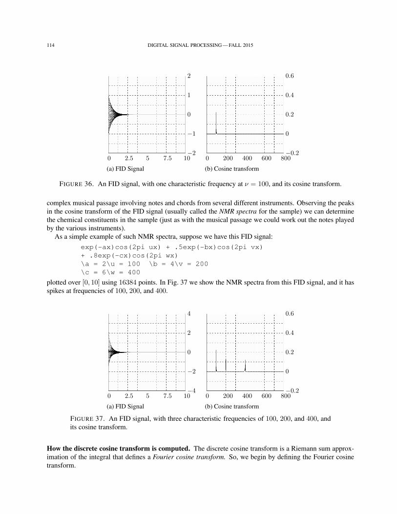
114 DIGITAL SIGNAL PROCESSING — FALL 2015
0 2.5 5 7.5 10−2
−1
0
1
2
(a) FID Signal
0 200 400 600 800−0.2
0
0.2
0.4
0.6
(b) Cosine transform
FIGURE 36. An FID signal, with one characteristic frequency at ν = 100, and its cosine transform.
complex musical passage involving notes and chords from several different instruments. Observing the peaks
in the cosine transform of the FID signal (usually called the NMR spectra for the sample) we can determine
the chemical constituents in the sample (just as with the musical passage we could work out the notes played
by the various instruments).
As a simple example of such NMR spectra, suppose we have this FID signal:
exp(-ax)cos(2pi ux) + .5exp(-bx)cos(2pi vx)
+ .8exp(-cx)cos(2pi wx)
\a = 2\u = 100 \b = 4\v = 200
\c = 6\w = 400
plotted over [0, 10] using 16384 points. In Fig. 37 we show the NMR spectra from this FID signal, and it has
spikes at frequencies of 100, 200, and 400.
0 2.5 5 7.5 10−4
−2
0
2
4
(a) FID Signal
0 200 400 600 800−0.2
0
0.2
0.4
0.6
(b) Cosine transform
FIGURE 37. An FID signal, with three characteristic frequencies of 100, 200, and 400, and
its cosine transform.
How the discrete cosine transform is computed. The discrete cosine transform is a Riemann sum approx-
imation of the integral that defines a Fourier cosine transform. So, we begin by defining the Fourier cosine
transform.
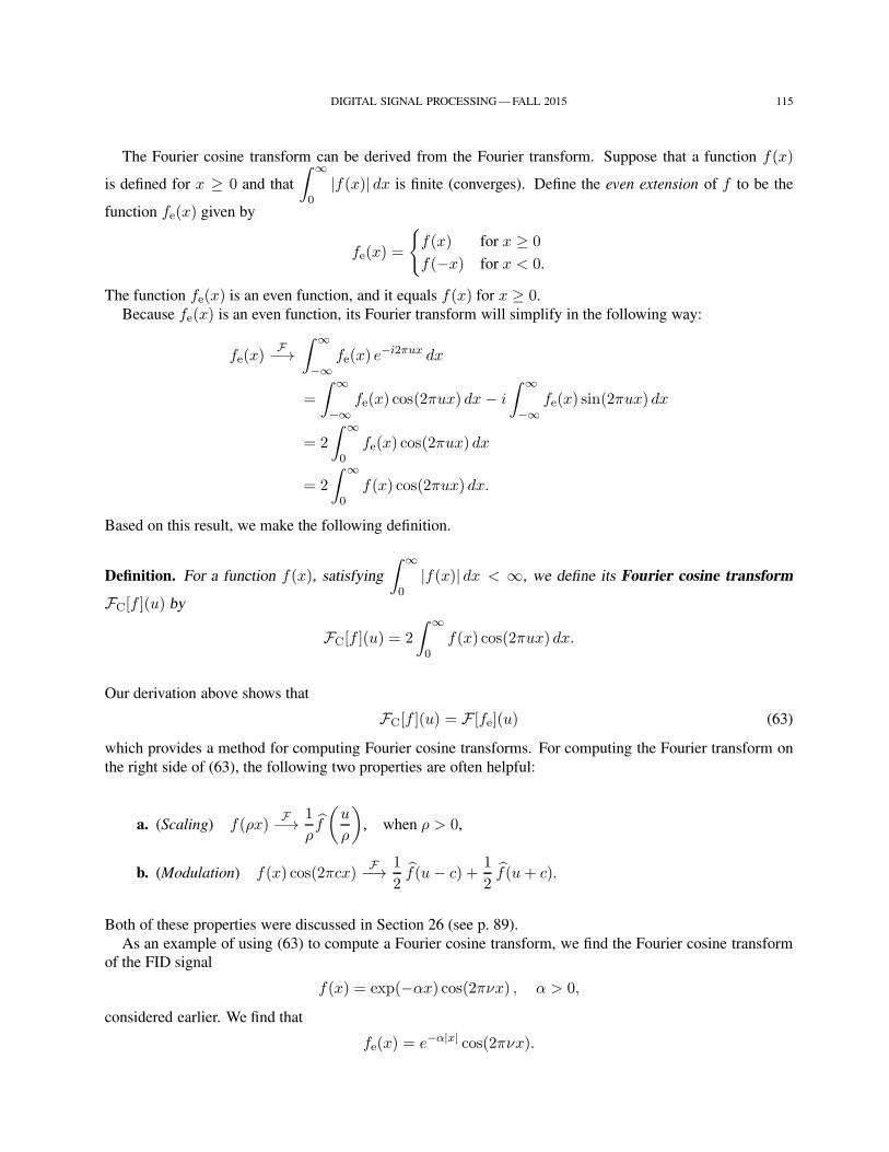
DIGITAL SIGNAL PROCESSING — FALL 2015 115
The Fourier cosine transform can be derived from the Fourier transform. Suppose that a function f(x)
is defined for x ≥ 0 and that
∫ ∞
0|f(x)| dx is finite (converges). Define the even extension of f to be the
function fe(x) given by
fe(x) =
f(x) for x ≥ 0
f(−x) for x < 0.
The function fe(x) is an even function, and it equals f(x) for x ≥ 0.
Because fe(x) is an even function, its Fourier transform will simplify in the following way:
fe(x)F−→∫ ∞
−∞fe(x) e
−i2πux dx
=
∫ ∞
−∞fe(x) cos(2πux) dx − i
∫ ∞
−∞fe(x) sin(2πux) dx
= 2
∫ ∞
0fe(x) cos(2πux) dx
= 2
∫ ∞
0f(x) cos(2πux) dx.
Based on this result, we make the following definition.
Definition. For a function f(x), satisfying
∫ ∞
0|f(x)| dx < ∞, we define its Fourier cosine transform
FC[f ](u) by
FC[f ](u) = 2
∫ ∞
0f(x) cos(2πux) dx.
Our derivation above shows that
FC[f ](u) = F [fe](u) (63)
which provides a method for computing Fourier cosine transforms. For computing the Fourier transform on
the right side of (63), the following two properties are often helpful:
a. (Scaling) f(ρx)F−→ 1
ρf
(u
ρ
), when ρ > 0,
b. (Modulation) f(x) cos(2πcx)F−→ 1
2f(u− c) +
1
2f(u+ c).
Both of these properties were discussed in Section 26 (see p. 89).
As an example of using (63) to compute a Fourier cosine transform, we find the Fourier cosine transform
of the FID signal
f(x) = exp(−αx) cos(2πνx) , α > 0,
considered earlier. We find that
fe(x) = e−α|x| cos(2πνx).
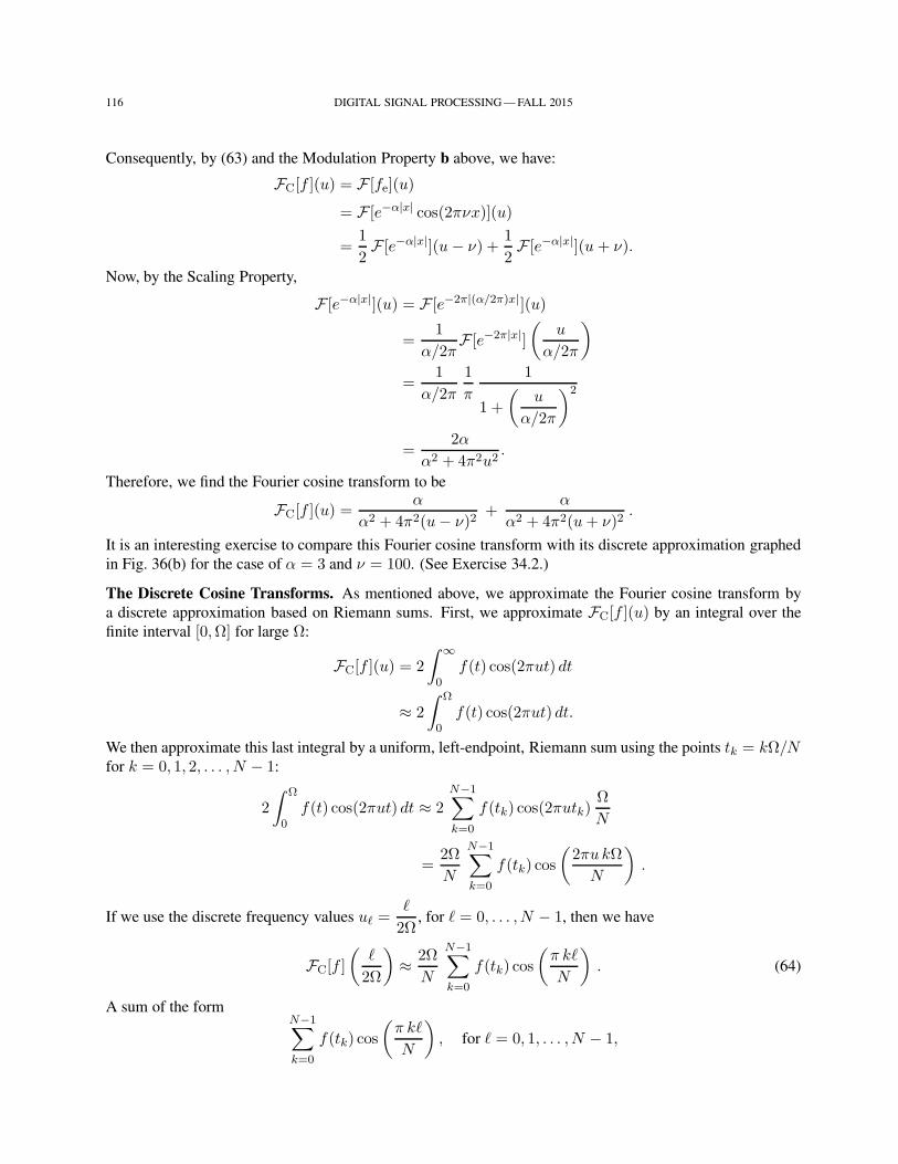
116 DIGITAL SIGNAL PROCESSING — FALL 2015
Consequently, by (63) and the Modulation Property b above, we have:
FC[f ](u) = F [fe](u)
= F [e−α|x| cos(2πνx)](u)
=1
2F [e−α|x|](u− ν) +
1
2F [e−α|x|](u+ ν).
Now, by the Scaling Property,
F [e−α|x|](u) = F [e−2π|(α/2π)x|](u)
=1
α/2πF [e−2π|x|]
(u
α/2π
)
=1
α/2π
1
π
1
1 +
(u
α/2π
)2
=2α
α2 + 4π2u2.
Therefore, we find the Fourier cosine transform to be
FC[f ](u) =α
α2 + 4π2(u− ν)2+
α
α2 + 4π2(u+ ν)2.
It is an interesting exercise to compare this Fourier cosine transform with its discrete approximation graphed
in Fig. 36(b) for the case of α = 3 and ν = 100. (See Exercise 34.2.)
The Discrete Cosine Transforms. As mentioned above, we approximate the Fourier cosine transform by
a discrete approximation based on Riemann sums. First, we approximate FC[f ](u) by an integral over the
finite interval [0,Ω] for large Ω:
FC[f ](u) = 2
∫ ∞
0f(t) cos(2πut) dt
≈ 2
∫ Ω
0f(t) cos(2πut) dt.
We then approximate this last integral by a uniform, left-endpoint, Riemann sum using the points tk = kΩ/Nfor k = 0, 1, 2, . . . , N − 1:
2
∫ Ω
0f(t) cos(2πut) dt ≈ 2
N−1∑
k=0
f(tk) cos(2πutk)Ω
N
=2Ω
N
N−1∑
k=0
f(tk) cos
(2πu kΩ
N
).
If we use the discrete frequency values uℓ =ℓ
2Ω, for ℓ = 0, . . . , N − 1, then we have
FC[f ]
(ℓ
2Ω
)≈ 2Ω
N
N−1∑
k=0
f(tk) cos
(π kℓ
N
). (64)
A sum of the formN−1∑
k=0
f(tk) cos
(π kℓ
N
), for ℓ = 0, 1, . . . , N − 1,
DIGITAL SIGNAL PROCESSING — FALL 2015 117
is a Discrete Cosine Transform of the data f(tk)N−1k=0 . It can be computed extremely rapidly using FFTs
along with some trigonometric identities. (For details, see Chapter 3 of Fast Fourier Transforms, 2nd Edition
by James S. Walker.)
Homework.
34.1. Find Fourier cosine transforms of the following functions:
(a)S rec(x− 2)
(b) f(x) = 2e−2x cos(20πx) + 5e−4x cos(80πx)
(c)S e−4πx2
(d) rec(x− 3) + rec(x− 5)
34.2. (a) Have FAWAV compute the Fourier cosine transform of e−3x cos(200πx) using an interval of [0, 10]and 16384 points. (b) Plot the exact Fourier cosine transform of this function over the interval [0, 819.2] and
compare (using Sup-norm difference) with the approximation found in (a). (c) Display the cosine transforms
found in (a) and (b) over the interval [90, 110].
34.3S . Use FAWAV to plot the cosine transform of the random data function rang(0) over the interval
[0, 10] using 16384 points. Then plot the cosine transform of this cosine transform, and compute its Sup-
norm difference with the original data. Note: This exercise illustrates that the discrete cosine transform is
also self-inversive, except for a negligible rounding error.
35. FOURIER TRANSFORM INFRARED SPECTROSCOPY
Fourier Transform Infrared Spectroscopy is another field where discrete cosine transforms are important.
The physical apparatus employed in this type of spectroscopy is called an interferometer. On the left of Fig. 38
we show a schematic diagram of an interferometer. A signal is passed through the sample, then through a
beam splitter which creates two signals, each traveling different routes before recombining and entering a
detector. For a good description of the physical background of interferometry, see the article at
http://en.wikipedia.org/wiki/Interferometer (65)
There is also a nice set of graphs of typical examples of Infrared Spectra obtained by this Fourier Transform
method at
https://www2.chemistry.msu.edu/faculty/reusch/VirtTxtJml/Spectrpy/InfraRed/infrared.htm#ir1 (66)
We now discuss the mathematics involved. Suppose that the signal entering the interferometer is f(t).Then by Fourier inversion we have
f(t) =
∫ ∞
−∞f(u)ei2πut du. (67)
The frequency spectrum |f(u)|2 is the most important quantity to find, since it is used to identify constituents
in the sample. The Fourier transform f(u) in Equation (67) is the transform of the signal after it has passed
through the sample. For this method to work, it is important that we have a signal entering the sample that has
a known transform. The best transform to have would be equal to 1 over the range of frequencies of interest.
It’s kind of a reverse analogy to a good frequency response function for an audio amplifier, but here we want a
good frequency profile for our probe signal. Due to the nature of the motions, and consequent absorptions of
energy, at infrared frequencies, a probe signal with infrared light is used—this is described well in the article
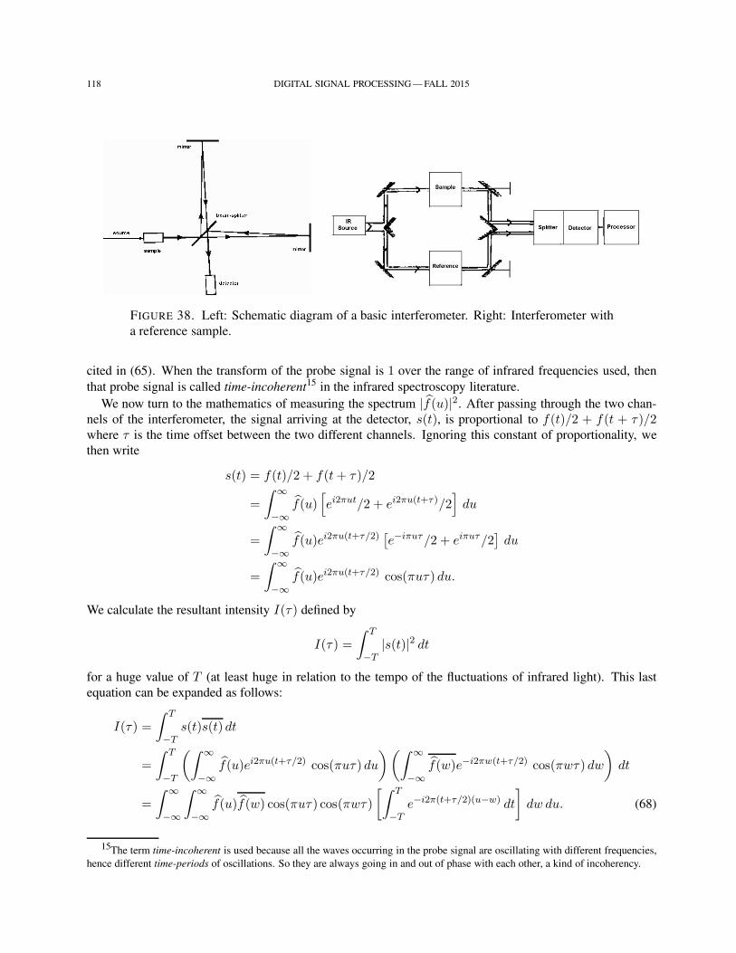
118 DIGITAL SIGNAL PROCESSING — FALL 2015
FIGURE 38. Left: Schematic diagram of a basic interferometer. Right: Interferometer with
a reference sample.
cited in (65). When the transform of the probe signal is 1 over the range of infrared frequencies used, then
that probe signal is called time-incoherent15 in the infrared spectroscopy literature.
We now turn to the mathematics of measuring the spectrum |f(u)|2. After passing through the two chan-
nels of the interferometer, the signal arriving at the detector, s(t), is proportional to f(t)/2 + f(t + τ)/2where τ is the time offset between the two different channels. Ignoring this constant of proportionality, we
then write
s(t) = f(t)/2 + f(t+ τ)/2
=
∫ ∞
−∞f(u)
[ei2πut/2 + ei2πu(t+τ)/2
]du
=
∫ ∞
−∞f(u)ei2πu(t+τ/2)
[e−iπuτ/2 + eiπuτ/2
]du
=
∫ ∞
−∞f(u)ei2πu(t+τ/2) cos(πuτ) du.
We calculate the resultant intensity I(τ) defined by
I(τ) =
∫ T
−T|s(t)|2 dt
for a huge value of T (at least huge in relation to the tempo of the fluctuations of infrared light). This last
equation can be expanded as follows:
I(τ) =
∫ T
−Ts(t)s(t) dt
=
∫ T
−T
(∫ ∞
−∞f(u)ei2πu(t+τ/2) cos(πuτ) du
)(∫ ∞
−∞f(w)e−i2πw(t+τ/2) cos(πwτ) dw
)dt
=
∫ ∞
−∞
∫ ∞
−∞f(u)f(w) cos(πuτ) cos(πwτ)
[∫ T
−Te−i2π(t+τ/2)(u−w) dt
]dw du. (68)
15The term time-incoherent is used because all the waves occurring in the probe signal are oscillating with different frequencies,
hence different time-periods of oscillations. So they are always going in and out of phase with each other, a kind of incoherency.
DIGITAL SIGNAL PROCESSING — FALL 2015 119
We now examine the integral in brackets above:
∫ T
−Te−i2π(t+τ/2)(u−w) dt (69)
using two different methods. The first method is the one typically used by physicists and other scientists. It is
not the most precise mathematically, but it does avoid some rather subtle mathematical manipulations, while
still arriving at the correct result. The second method uses standard methods from the world of mathematics.
Method 1. For the integral in (69) we consider two cases. First, suppose u = w, we then have
∫ T
−Te−i2π(t+τ/2)(u−w) dt =
∫ T
−Te0 dt
= 2T.
On the other hand, if u 6= w, then
∫ T
−Te−i2π(t+τ/2)(u−w) dt ≈ 0 (at least, relative to 2T )
due to the large amount of cancellation of the real and imaginary parts of the integral (which are integrals of
cosines and sines). Hence, for very large T , we have (writing our approximation as equality):
∫ T
−Te−i2π(t+τ/2)(u−w) dt =
∞, if u = w
0, if u 6= w
= δ(u− w)
where we have introduced Dirac’s delta function. Based on this last result, we rewrite (68) as follows:
I(τ) =
∫ ∞
−∞
∫ ∞
−∞f(u)f(w) cos(πuτ) cos(πwτ) δ(u − w) dw du
=
∫ ∞
−∞f(u)f(u) cos(πuτ) cos(πuτ) du
=
∫ ∞
−∞|f(u)|2 cos2(πuτ) du.
Thus, we have obtained the important equation
I(τ) =
∫ ∞
−∞|f(u)|2 cos2(πuτ) du. (70)
Method 2. The previous derivation was not too precise mathematically (and also introduced the Dirac delta
function, which some readers may not be too comfortable with). We now derive (70) using a mathematically
precise argument. Since
e−i2π(t+τ/2)(u−w) = e−iπτueiπτw e−i2πt(u−w)
120 DIGITAL SIGNAL PROCESSING — FALL 2015
we can rewrite (69) as follows:
∫ T
−Te−i2π(t+τ/2)(u−w) dt = e−iπτueiπτw
∫ T
−Te−i2πt(u−w) dt
= e−iπτueiπτw∫ T
−Tcos 2πt(u− w) dt
= e−iπτueiπτw∫ T
−Tcos 2πt(w − u) dt (cos is even)
= e−iπτueiπτw∫ T
−Te−i2πt(w−u) dt.
Substituting from this result into (68), we obtain (using e−i2πt(w−u) = e−i2πtwei2πtu and some rearranging
of the order of the integrals):
I(τ) =
∫ ∞
−∞
∫ ∞
−∞f(u)f(w) cos(πuτ) cos(πwτ)
[e−iπτueiπτw
∫ T
−Te−i2πt(w−u) dt
]dw du
=
∫ ∞
−∞f(u) cos(πuτ)e−iπτu
[∫ T
−T
(∫ ∞
−∞f(w) cos(πwτ)eiπτwe−i2πtw dw
)ei2πtu dt
]du.
Now, we examine the integral in brackets inside the last line. For very large T , by approximate Fourier
inversion, we have:
∫ T
−T
(∫ ∞
−∞f(w) cos(πwτ)eiπτwe−i2πtw dw
)ei2πtu dt
≈∫ ∞
−∞
(∫ ∞
−∞f(w) cos(πwτ)eiπτwe−i2πtw dw
)ei2πtu dt
= f(u) cos(πuτ)eiπτu
and so I(τ) is then (ignoring approximation):
I(τ) =
∫ ∞
−∞f(u) cos(πuτ)e−iπτu f(u) cos(πuτ)eiπτu du
=
∫ ∞
−∞|f(u)|2 cos2(πuτ) du.
We have again obtained Equation (70), but this time using more precise mathematics.
Cosine Transforms and Spectroscopy. The results we have found can be phrased in terms of a cosine
transform, and then an Infrared Spectrogram can be constructed using an inversion theorem for the cosine
transform. To get a cosine transform expression, we use the following trigonometric identity
cos2 θ =1
2+
1
2cos 2θ
in Equation (70) to obtain
I(τ) =1
2
∫ ∞
−∞|f(u)|2[1 + cos(2πuτ)] du.
DIGITAL SIGNAL PROCESSING — FALL 2015 121
Now, because the source signal f(t) is real-valued, we have |f(u)|2 = |f(−u)|2. (See Exercise 35.1.)
Therefore, by evenness of the integrand on the right side of this last equation, we obtain
I(τ) =
∫ ∞
0|f(u)|2[1 + cos(2πuτ)] du
=
∫ ∞
0|f(u)|2 du+
∫ ∞
0|f(u)|2 cos(2πuτ) du
=1
2
[I(0) + FC[|f(u)|2](τ)
].
Where we have introduced the constant I(0) for the integral 2∫∞0 |f(u)|2 du. From this last result we then
have the following formula for the Fourier cosine transform of the power spectrum |f(u)|2:
2I(τ) − I(0) = FC[|f(u)|2](τ). (71)
Equation (71) shows that we can obtain the power spectrum, |f(u)|2, provided we can invert the Fourier
cosine transform. Theoretically, we can do this by the inversion formula that we prove below. But that
formula requires the values of FC[|f(u)|2](τ) at all values of τ from 0 to ∞. That is not practical. But, with
discrete Fourier methods (based, ultimately, on the FFT) we can approximate the inversion process if we have
a large number of discrete values τk where we have made our interference measurements:
2I(τk)− I(0) = FC[|f(u)|2](τk), for k = 0, 1, . . . , N − 1. (72)
We can then approximate the inversion by similar reasoning as we used for NMR spectroscopy.
The measurements described by Equation (72) are performed by having one of the mirrors in the interfer-
ence apparatus slide through a sequence of positions (which correspond to different time offsets τk). For each
successive position, corresponding to a τk value, a measurement of I(τk) is made.
We now describe how, theoretically, the Fourier cosine transform in Equation (71) is inverted. The follow-
ing theorem shows that the inversion process simply consists of a second application of the Fourier cosine
transform. The Fourier cosine transform is said to be self-inverting.
Theorem [Inversion of Fourier cosine transform]. If g(x) is a regular function, and∫∞0 |g(x)| dx < ∞,
then for all x ≥ 0 we have
g(x) = 2
∫ ∞
0FC[g](u) cos(2πux) du.
Proof. We know that FC[g](u) = F [ge](u) and, by Fourier inversion, we have
ge(x) =
∫ ∞
−∞F [ge](u)e
i2πux du
=
∫ ∞
−∞FC[g](u)e
i2πux du.
Note that in this last integral we are using both positive and negative values of u, but the Fourier cosine
transform
FC[g](u) = 2
∫ ∞
0g(x) cos(2πux) dx
is clearly defined for all values of u. In fact, since cos(2πux) is an even function of u, it follows that FC[g](u)is also an even function of u. But then, by repeating our work above in defining the Fourier cosine transform,
122 DIGITAL SIGNAL PROCESSING — FALL 2015
it follows that
ge(x) =
∫ ∞
−∞FC[g](u)e
i2πux du
= 2
∫ ∞
0FC[g](u) cos(2πux) du.
Since ge(x) = g(x) for x ≥ 0, we have
g(x) = 2
∫ ∞
0FC[g](u) cos(2πux) du
for all x ≥ 0, and our theorem is proved.
Since the Fourier cosine transform is self-inversive, we can obtain |f(u)|2 from Equation (71) by applying
another Fourier cosine transform:
|f(u)|2 = 2
∫ ∞
0FC[|f(u)|2](τ) cos(2πτu) dτ
= 2
∫ ∞
0[2I(τ) − I(0)] cos(2πτu) dτ.
By repeating the discretization arguments that we used above to get Equation (64), we obtain the following
discrete approximation to this last formula:
∣∣∣∣f(
ℓ
2Ω
)∣∣∣∣2
≈ 2Ω
N
N−1∑
k=0
[2I(τk)− I(0)] cos
(π kℓ
N
). (73)
with τk = kΩ/N , for k = 0, 1, . . . , N − 1, and ℓ = 0, 1, . . . , N − 1.
Formula (73), along with FFT methods that are used to rapidly compute it, is the basis for Infrared Fourier
Transform Spectroscopy. We conclude our discussion with a few practical remarks on implementation. First,
we observe that to obtain (73), we used the approximation
2
∫ ∞
0[2I(τ) − I(0)] cos(2πτu) dτ ≈ 2
∫ Ω
0[2I(τ) − I(0)] cos(2πτu) dτ.
The sharp cutoff at τ = Ω on the integral on the right can cause distortions (ringing) in the approximation of
|f(u)|2. To reduce these distortions, an apodization factor A(τ) is introduced that gently damps down to 0 at
τ = Ω:
2
∫ Ω
0[2I(τ) − I(0)]A(τ) cos(2πτu) dτ.
For example, a hanning apodization factor
A(τ) = 0.5 + 0.5 cos(πτ/Ω)
could be used. This technique of apodization is closely analogous to the windowing used in calculating
spectrograms.
Second, we have only described the most basic method of Infrared Fourier Transform Spectroscopy. An-
other method that is more sophisticated—but not always practical—is to employ a second spectroscopic
analysis of a reference (or control) simultaneously with the analysis of the sample. We show a diagram of
this method on the right of Fig. 38. For example, this reference might consist of only the solvent in which the
sample is dissolved. This method helps to identify just the peaks in the spectrum of the sample, rather than
extraneous peaks from the solvent.
DIGITAL SIGNAL PROCESSING — FALL 2015 123
Finally, there is nothing sacrosanct about the use of infrared light for the probe. The method we have
described here applies just as well to other types of radiation for the probe. All such methods fall under the
rubric, Fourier Transform Spectroscopy.
Homework.
35.1S . Show that for a real-valued signal f(t), the power spectrum is even: |f(−u)|2 = |f(u)|2. [Hint:
First, show that f(−u) = f(u).]
35.2. (a)H Show that
2
∫ Ω
0[2I(τ) − I(0)] cos(2πτu) dτ = (|f |2 ∗ S)(u)
where S(u) = 2Ω sinc(2Ωu). (b) Use the result of (a) to explain why there will sometimes be distortion
(ringing) in the computation of the infrared Fourier transform spectrogram if no apodization is done.
SOLUTIONS TO SELECTED EXERCISES
2.1. (1):
∫ π
−πsinnx sinmxdx =
∫ π
−π
1
2cos(n −m)x− 1
2cos(n+m)x dx
=1
2(n−m)sin(n−m)x− 1
2(n +m)sin(n+m)x
∣∣∣∣π
−π
= 0 (sin kπ = 0, for k = 0,±1,±2, . . . ).
(2):
∫ π
−π1 · cosnx dx =
−1
nsinnx
∣∣∣∣π
−π
= 0
∫ π
−π1 · sinnx dx =
− cosnx
n
∣∣∣∣π
−π
=− cosnπ
n+
cosnπ
n= 0
∫ π
−π12 dx = x
∣∣π−π
= 2π.
(3):
∫ π
−πsin2 nx dx =
∫ π
−π
1
2− 1
2cos 2nx dx
=x
2− 1
2nsin 2nx
∣∣∣∣π
−π
= π.
124 DIGITAL SIGNAL PROCESSING — FALL 2015
2.2. (a) For c0, we have
c0 =1
2π
∫ π
−πf(x) dx
=1
2π
∫ π
π/21 dx
= 1.
For An, we have
An =1
π
∫ π
−πf(x) cosnx dx
=1
π
∫ π
π/2cosnx dx
=1
π
sinnx
n
∣∣∣∣π
π/2
=− sin(nπ/2)
nπ.
For Bn, we have
Bn =1
π
∫ π
−πf(x) sinnx dx
=1
π
∫ π
π/2sinnx dx
=− cosnx
nπ
∣∣∣∣π
π/2
=cos(nπ/2)− cos(nπ)
nπ.
Therefore, the Fourier series for f(x) is
1 +
∞∑
n=1
[cos(nπ/2)− cos(nπ)
nπsinnx− sin(nπ/2)
nπcosnx
].
(e) Use the identity 2 sin2 x = 1− sin(2x). The orthogonality theorem also plays a role.
DIGITAL SIGNAL PROCESSING — FALL 2015 125
2.3. We have∫ π
0sinnx sinmxdx =
∫ π
0
1
2cos(n−m)x− 1
2cos(n+m)x dx
=1
2(n−m)sin(n−m)x− 1
2(n +m)sin(n+m)x
∣∣∣∣π
0
= 0 (when n 6= m)
or
=
∫ π
0
1
2− 1
2cos 2nx dx (if n = m)
=x
2− 1
2nsin 2nx
∣∣∣∣π
0
=π
2.
2.4. Multiplying by sinnx and integrating, while remembering to change
∞∑
n=1
to
∞∑
m=1
, we obtain
∫ π
0f(x) sinnx dx =
∫ π
0
∞∑
m=1
Bm sinmx sinnx dx
=
∞∑
m=1
Bm
∫ π
0sinmx sinnx dx (assuming term by term integration is valid)
= Bn · π/2 (all other terms, for m 6= n, are 0).
Therefore, we obtain the following formula for Bn:
Bn =2
π
∫ π
0f(x) sinnx dx.
2.5. (a) Using the formula from problem 2.4, we have
Bn =2
π
∫ π
0f(x) sinnx dx
=2
π
∫ π
π/21 · sinnx dx
=2
π
− cosnx
n
∣∣∣∣π
π/2
=2[cos(nπ/2)− cos(nπ)
]
nπ.
Therefore, the Fourier sine series for f(x) is
∞∑
n=1
2[cos(nπ/2)− cos(nπ)
]
nπsinnx.
126 DIGITAL SIGNAL PROCESSING — FALL 2015
2.6. (a):
∫ π
0cosnx cosmxdx =
∫ π
0
1
2cos(n−m)x+
1
2cos(n+m)x dx
=1
2(n −m)sin(n−m)x+
1
2(n +m)sin(n+m)x
∣∣∣∣π
0
= 0 (when n 6= m)
or
=
∫ π
0
1
2+
1
2cos 2nx dx (if n = m)
=x
2+
1
2nsin 2nx
∣∣∣∣π
0
=π
2.
(b):
∫ π
01 · cosnx dx =
sinnx
n
∣∣∣∣π
0
= 0
(c):
∫ π
012 dx = x|π0 = π.
2.7. For c0, integrate both sides. For An, multiply both sides by cosnx and integrate (proceeding similarly
to the solution to problem 2.4).
3.1. (b):
c0 =1
10
∫ 5
−5|x|+ 2 dx
=1
5
∫ 5
0x+ 2 dx
=1
5(x2/2 + 2x)
∣∣∣∣5
0
=1
5(25/2 + 10)
=9
2,
An =1
5
∫ 5
−5(|x|+ 2) cos
nπx
5dx
=2
5
∫ 5
0(x+ 2) cos
nπx
5dx
=2
nπ(x+ 2) sin
nπx
5
∣∣∣∣5
0
+10
n2π2cos
nπx
5
∣∣∣∣5
0
= 0 +10
n2π2(cosnπ − 1),
Bn =1
5
∫ 5
−5(|x|+ 2) sin
nπx
5dx
= 0.
DIGITAL SIGNAL PROCESSING — FALL 2015 127
So the Fourier series is
9
2+
∞∑
n=1
10(cos nπ − 1)
n2π2cos
nπx
5.
(c):
c0 =1
π
∫ π/2
−π/2sinx dx = 0,
An =2
π
∫ π/2
−π/2sinx cos 2nx dx = 0,
Bn =2
π
∫ π/2
−π/2sinx sin 2nx dx
=4
π
∫ π/2
0sinx sin 2nx dx
=
∫ π/2
0
( 2π
cos(2n − 1)x− 2
πcos(2n+ 1)x
)dx
=2
(2n − 1)πsin(2n− 1)x
∣∣∣∣π/2
0
− 2
(2n+ 1)πsin(2n + 1)x
∣∣∣∣π/2
0
=2 sin(nπ − π/2)
(2n − 1)π− 2 sin(nπ + π/2)
(2n+ 1)π
=−2 cosnπ
(2n − 1)π− 2 cos nπ
(2n+ 1)π
= (−1)n+1 8n
(4n2 − 1)π.
So the Fourier series is∞∑
n=1
(−1)n+1 8n
(4n2 − 1)πsin 2nx.
3.2. To derive c0, integrate
f(x) = c0 +∞∑
n=1
[An cosnπx
a+Bn sin
nπx
a] (74)
from −a to a, term by term, obtaining
∫ a
−af(x) dx =
∫ a
−ac0 dx+
∞∑
n=1
[An
∫ a
−acos
nπx
adx+Bn
∫ a
−asin
nπx
adx]
= 2ac0 +
∞∑
n=1
(0 + 0)
= 2ac0.
Therefore, c0 =1
2a
∫ a
−af(x) dx.
128 DIGITAL SIGNAL PROCESSING — FALL 2015
To derive An, multiply (74) by cosnπx
aand integrate term by term:
∫ a
−af(x) cos
nπx
adx =
∫ a
−ac0 cos
nπx
adx
+∞∑
m=1
[Am
∫ a
−acos
mπx
acos
nπx
adx+Bm
∫ a
−asin
mπx
acos
nπx
adx]
= 0 +( ∞∑
m=1m6=n
Am 0)+An
∫ a
−acos2
nπx
adx+
∞∑
m=1
Bm 0
= An a.
Therefore, An =1
a
∫ a
−af(x) cos
nπx
adx. A similar argument shows that Bn =
1
a
∫ a
−af(x) sin
nπx
adx.
3.3. Suppose f(x) = 1 and g(x) = cosnπx
a. Then
∫ a
0f(x)g(x) dx =
∫ a
01 · cos nπx
adx
= sinnπx
a
∣∣∣a
0= 0.
If f(x) = cosnπx
aand g(x) = cos
mπx
afor m 6= n, then
∫ a
0f(x)g(x) dx =
∫ a
0cos
nπx
acos
mπx
adx
=
∫ a
0
(12cos
(n+m)πx
a+
1
2cos
(n−m)πx
a
)dx
=1
2(n +m)πsin
(n+m)πx
a+
1
2(n −m)πsin
(n−m)πx
a
∣∣∣∣a
0
= 0.
Finally, we have∫ a0 12 dx = a, and
∫ a
0cos2
nπx
adx =
∫ a
0
1
2+
1
2cos
2nπx
adx
=x
2+
a
4nπsin
2nπx
a
∣∣∣∣a
0
=a
2.
3.4. To derive c0, integrate the following equation, term-by-term:
f(x) = c0 +∞∑
n=1
An cosnπx
a(75)
DIGITAL SIGNAL PROCESSING — FALL 2015 129
obtaining
∫ a
0f(x) dx =
∫ a
0c0 dx+
∞∑
n=1
An
∫ a
0cos
nπx
adx
= c0a+ 0.
Therefore, c0 =1
a
∫ a
0f(x) dx.
To derive An, multiply (75) by cosnπx
aand integrate term by term:
∫ a
0f(x) cos
nπx
adx =
∫ a
0c0 cos
nπx
adx+
∞∑
m=1
Am
∫ a
0cos
mπx
acos
nπx
adx
= Ana
2(using theorem from Exercise 3.3).
Therefore, An =2
a
∫ a
0f(x) cos
nπx
adx.
3.6. Multiplying by sin(nπx/a) and integrating, while remembering to change
∞∑
n=1
to
∞∑
m=1
, we obtain
∫ a
0f(x) sin(nπx/a) dx =
∫ a
0
∞∑
m=1
Bm sin(mπx/a) sin(nπx/a) dx
=
∞∑
m=1
Bm
∫ a
0sin(mπx/a) sin(nπx/a) dx (using term by term integration)
= Bn · a/2 (all other terms, for m 6= n, are 0).
Therefore, we obtain the following formula for Bn:
Bn =2
a
∫ a
0f(x) sin(nπx/a) dx.
3.7. (a) For c0, using a = 4, we calculate as follows
c0 =1
4
∫ 4
0f(x) dx
=1
4
∫ 3
11 dx
=1
2.
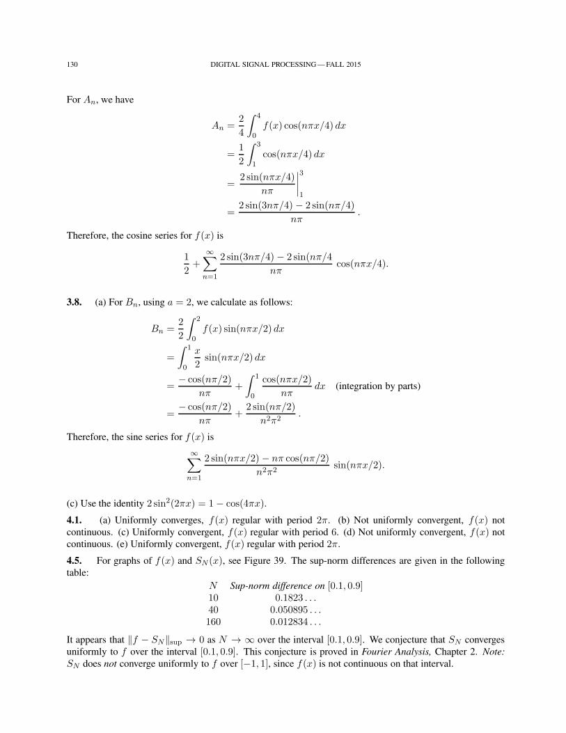
130 DIGITAL SIGNAL PROCESSING — FALL 2015
For An, we have
An =2
4
∫ 4
0f(x) cos(nπx/4) dx
=1
2
∫ 3
1cos(nπx/4) dx
=2 sin(nπx/4)
nπ
∣∣∣∣3
1
=2 sin(3nπ/4) − 2 sin(nπ/4)
nπ.
Therefore, the cosine series for f(x) is
1
2+
∞∑
n=1
2 sin(3nπ/4) − 2 sin(nπ/4
nπcos(nπx/4).
3.8. (a) For Bn, using a = 2, we calculate as follows:
Bn =2
2
∫ 2
0f(x) sin(nπx/2) dx
=
∫ 1
0
x
2sin(nπx/2) dx
=− cos(nπ/2)
nπ+
∫ 1
0
cos(nπx/2)
nπdx (integration by parts)
=− cos(nπ/2)
nπ+
2 sin(nπ/2)
n2π2.
Therefore, the sine series for f(x) is
∞∑
n=1
2 sin(nπx/2)− nπ cos(nπ/2)
n2π2sin(nπx/2).
(c) Use the identity 2 sin2(2πx) = 1− cos(4πx).
4.1. (a) Uniformly converges, f(x) regular with period 2π. (b) Not uniformly convergent, f(x) not
continuous. (c) Uniformly convergent, f(x) regular with period 6. (d) Not uniformly convergent, f(x) not
continuous. (e) Uniformly convergent, f(x) regular with period 2π.
4.5. For graphs of f(x) and SN (x), see Figure 39. The sup-norm differences are given in the following
table:
N Sup-norm difference on [0.1, 0.9]10 0.1823 . . .40 0.050895 . . .160 0.012834 . . .
It appears that ‖f − SN‖sup → 0 as N → ∞ over the interval [0.1, 0.9]. We conjecture that SN converges
uniformly to f over the interval [0.1, 0.9]. This conjecture is proved in Fourier Analysis, Chapter 2. Note:
SN does not converge uniformly to f over [−1, 1], since f(x) is not continuous on that interval.
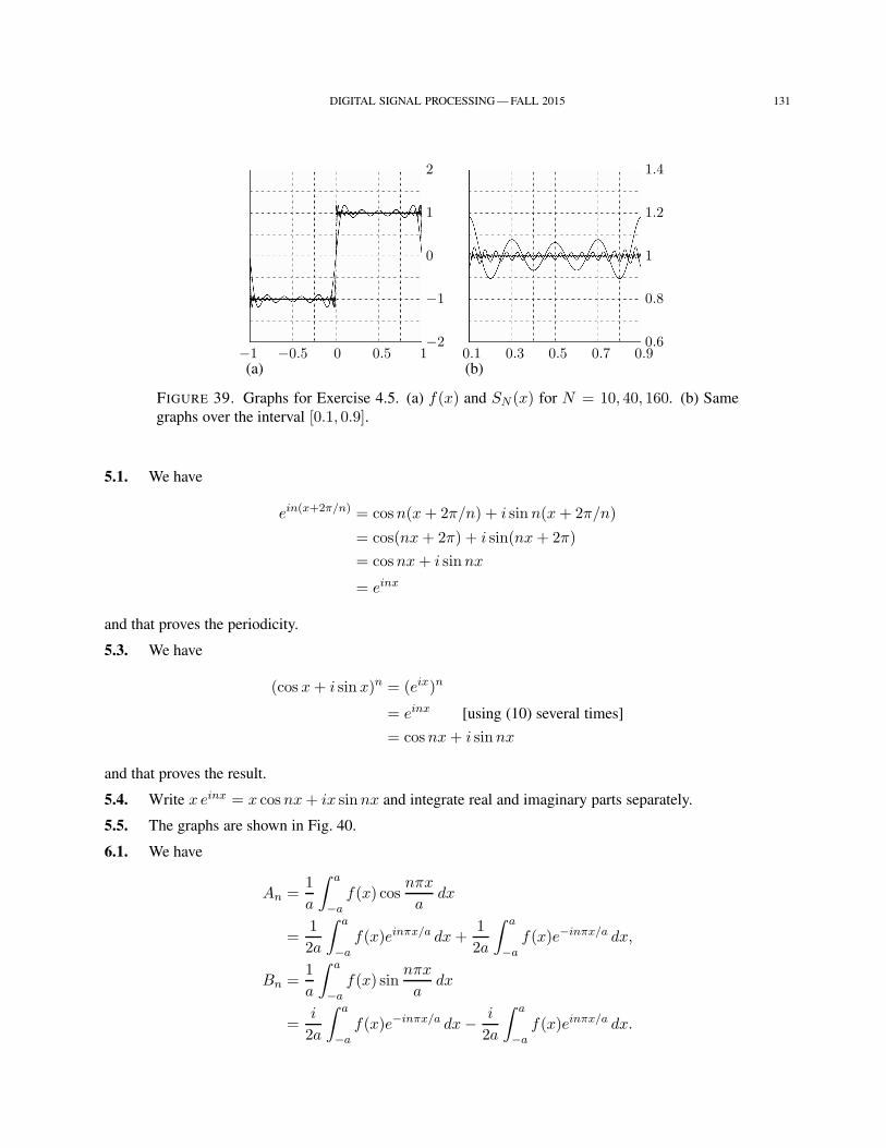
DIGITAL SIGNAL PROCESSING — FALL 2015 131
−1 −0.5 0 0.5 1−2
−1
0
1
2
(a)0.1 0.3 0.5 0.7 0.9
0.6
0.8
1
1.2
1.4
(b)
FIGURE 39. Graphs for Exercise 4.5. (a) f(x) and SN (x) for N = 10, 40, 160. (b) Same
graphs over the interval [0.1, 0.9].
5.1. We have
ein(x+2π/n) = cosn(x+ 2π/n) + i sin n(x+ 2π/n)
= cos(nx+ 2π) + i sin(nx+ 2π)
= cosnx+ i sinnx
= einx
and that proves the periodicity.
5.3. We have
(cos x+ i sinx)n = (eix)n
= einx [using (10) several times]
= cosnx+ i sinnx
and that proves the result.
5.4. Write x einx = x cosnx+ ix sinnx and integrate real and imaginary parts separately.
5.5. The graphs are shown in Fig. 40.
6.1. We have
An =1
a
∫ a
−af(x) cos
nπx
adx
=1
2a
∫ a
−af(x)einπx/a dx+
1
2a
∫ a
−af(x)e−inπx/a dx,
Bn =1
a
∫ a
−af(x) sin
nπx
adx
=i
2a
∫ a
−af(x)e−inπx/a dx− i
2a
∫ a
−af(x)einπx/a dx.
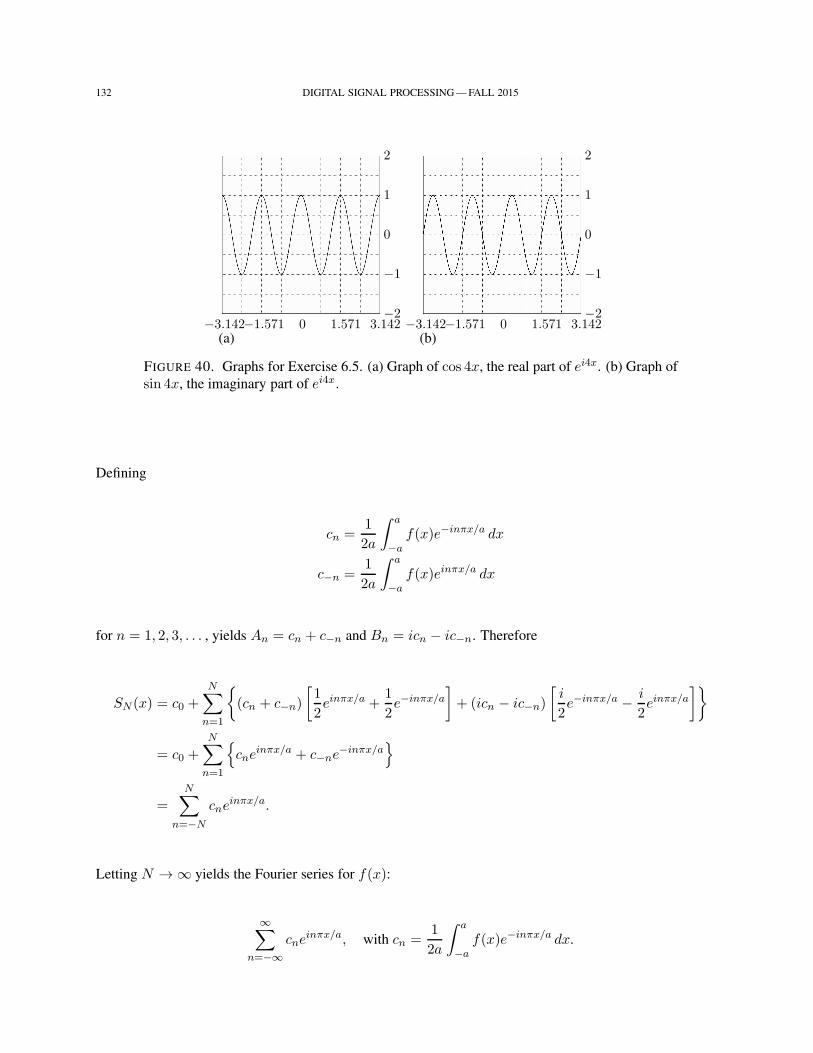
132 DIGITAL SIGNAL PROCESSING — FALL 2015
−3.142−1.571 0 1.571 3.142−2
−1
0
1
2
(a)−3.142−1.571 0 1.571 3.142
−2
−1
0
1
2
(b)
FIGURE 40. Graphs for Exercise 6.5. (a) Graph of cos 4x, the real part of ei4x. (b) Graph of
sin 4x, the imaginary part of ei4x.
Defining
cn =1
2a
∫ a
−af(x)e−inπx/a dx
c−n =1
2a
∫ a
−af(x)einπx/a dx
for n = 1, 2, 3, . . . , yields An = cn + c−n and Bn = icn − ic−n. Therefore
SN (x) = c0 +
N∑
n=1
(cn + c−n)
[1
2einπx/a +
1
2e−inπx/a
]+ (icn − ic−n)
[i
2e−inπx/a − i
2einπx/a
]
= c0 +
N∑
n=1
cne
inπx/a + c−ne−inπx/a
=
N∑
n=−N
cneinπx/a.
Letting N → ∞ yields the Fourier series for f(x):
∞∑
n=−∞cne
inπx/a, with cn =1
2a
∫ a
−af(x)e−inπx/a dx.
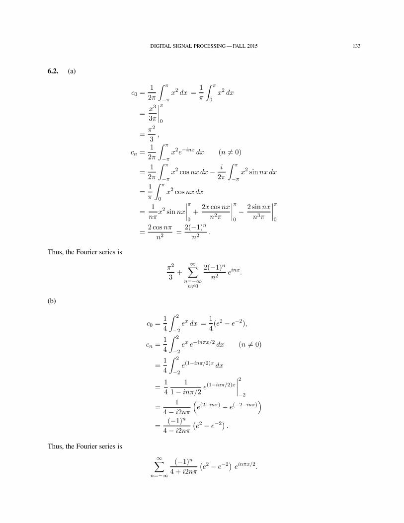
DIGITAL SIGNAL PROCESSING — FALL 2015 133
6.2. (a)
c0 =1
2π
∫ π
−πx2 dx =
1
π
∫ π
0x2 dx
=x3
3π
∣∣∣∣π
0
=π2
3,
cn =1
2π
∫ π
−πx2e−inx dx (n 6= 0)
=1
2π
∫ π
−πx2 cosnx dx− i
2π
∫ π
−πx2 sinnx dx
=1
π
∫ π
0x2 cosnx dx
=1
nπx2 sinnx
∣∣∣∣π
0
+2x cosnx
n2π
∣∣∣∣π
0
− 2 sinnx
n3π
∣∣∣∣π
0
=2cosnπ
n2=
2(−1)n
n2.
Thus, the Fourier series is
π2
3+
∞∑
n=−∞n 6=0
2(−1)n
n2einx.
(b)
c0 =1
4
∫ 2
−2ex dx =
1
4(e2 − e−2),
cn =1
4
∫ 2
−2ex e−inπx/2 dx (n 6= 0)
=1
4
∫ 2
−2e(1−inπ/2)x dx
=1
4
1
1− inπ/2e(1−inπ/2)x
∣∣∣∣2
−2
=1
4− i2nπ
(e(2−inπ) − e(−2−inπ)
)
=(−1)n
4− i2nπ
(e2 − e−2
).
Thus, the Fourier series is
∞∑
n=−∞
(−1)n
4 + i2nπ
(e2 − e−2
)einπx/2.
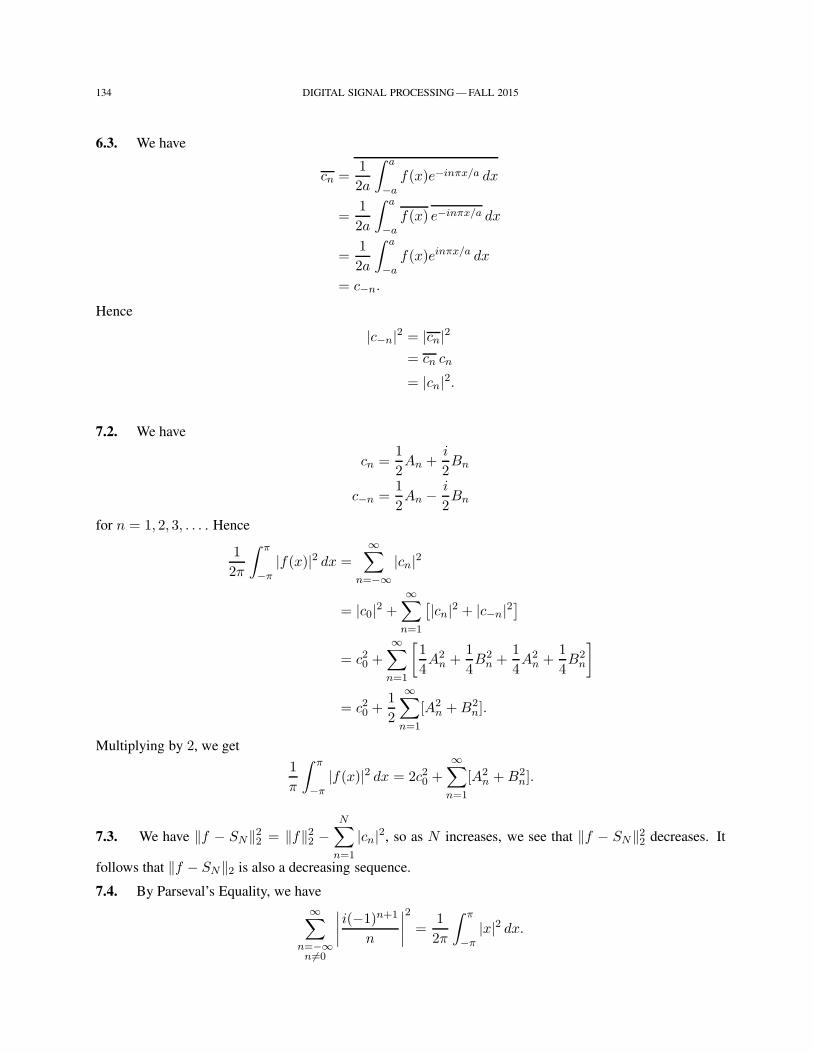
134 DIGITAL SIGNAL PROCESSING — FALL 2015
6.3. We have
cn =1
2a
∫ a
−af(x)e−inπx/a dx
=1
2a
∫ a
−af(x) e−inπx/a dx
=1
2a
∫ a
−af(x)einπx/a dx
= c−n.
Hence
|c−n|2 = |cn|2= cn cn
= |cn|2.
7.2. We have
cn =1
2An +
i
2Bn
c−n =1
2An − i
2Bn
for n = 1, 2, 3, . . . . Hence
1
2π
∫ π
−π|f(x)|2 dx =
∞∑
n=−∞|cn|2
= |c0|2 +∞∑
n=1
[|cn|2 + |c−n|2
]
= c20 +
∞∑
n=1
[1
4A2
n +1
4B2
n +1
4A2
n +1
4B2
n
]
= c20 +1
2
∞∑
n=1
[A2n +B2
n].
Multiplying by 2, we get
1
π
∫ π
−π|f(x)|2 dx = 2c20 +
∞∑
n=1
[A2n +B2
n].
7.3. We have ‖f − SN‖22 = ‖f‖22 −N∑
n=1
|cn|2, so as N increases, we see that ‖f − SN‖22 decreases. It
follows that ‖f − SN‖2 is also a decreasing sequence.
7.4. By Parseval’s Equality, we have
∞∑
n=−∞n 6=0
∣∣∣∣i(−1)n+1
n
∣∣∣∣2
=1
2π
∫ π
−π|x|2 dx.
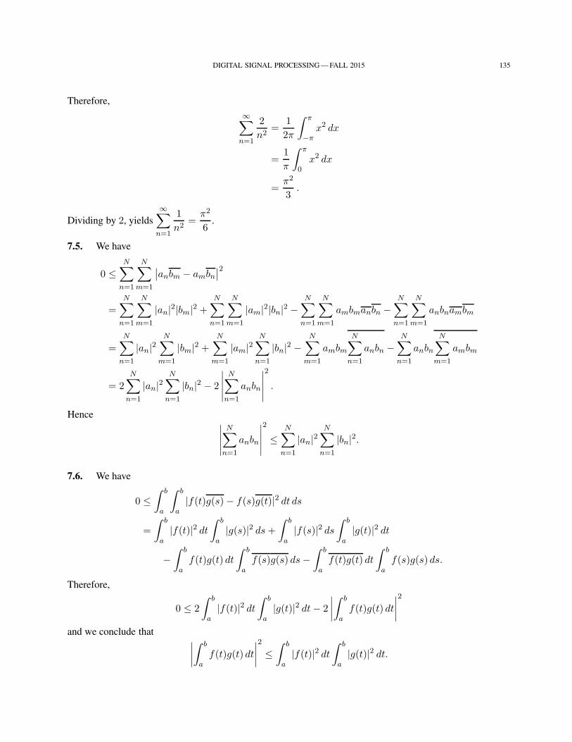
DIGITAL SIGNAL PROCESSING — FALL 2015 135
Therefore,
∞∑
n=1
2
n2=
1
2π
∫ π
−πx2 dx
=1
π
∫ π
0x2 dx
=π2
3.
Dividing by 2, yields
∞∑
n=1
1
n2=
π2
6.
7.5. We have
0 ≤N∑
n=1
N∑
m=1
∣∣anbm − ambn∣∣2
=N∑
n=1
N∑
m=1
|an|2|bm|2 +N∑
n=1
N∑
m=1
|am|2|bn|2 −N∑
n=1
N∑
m=1
ambmanbn −N∑
n=1
N∑
m=1
anbnambm
=
N∑
n=1
|an|2N∑
m=1
|bm|2 +N∑
m=1
|am|2N∑
n=1
|bn|2 −N∑
m=1
ambm
N∑
n=1
anbn −N∑
n=1
anbn
N∑
m=1
ambm
= 2
N∑
n=1
|an|2N∑
n=1
|bn|2 − 2
∣∣∣∣∣N∑
n=1
anbn
∣∣∣∣∣
2
.
Hence ∣∣∣∣∣N∑
n=1
anbn
∣∣∣∣∣
2
≤N∑
n=1
|an|2N∑
n=1
|bn|2.
7.6. We have
0 ≤∫ b
a
∫ b
a|f(t)g(s)− f(s)g(t)|2 dt ds
=
∫ b
a|f(t)|2 dt
∫ b
a|g(s)|2 ds+
∫ b
a|f(s)|2 ds
∫ b
a|g(t)|2 dt
−∫ b
af(t)g(t) dt
∫ b
af(s)g(s) ds−
∫ b
af(t)g(t) dt
∫ b
af(s)g(s) ds.
Therefore,
0 ≤ 2
∫ b
a|f(t)|2 dt
∫ b
a|g(t)|2 dt− 2
∣∣∣∣∫ b
af(t)g(t) dt
∣∣∣∣2
and we conclude that ∣∣∣∣∫ b
af(t)g(t) dt
∣∣∣∣2
≤∫ b
a|f(t)|2 dt
∫ b
a|g(t)|2 dt.
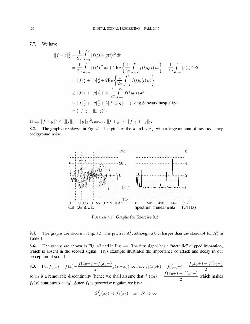
136 DIGITAL SIGNAL PROCESSING — FALL 2015
7.7. We have
‖f + g‖22 =1
2a
∫ a
−a|f(t) + g(t)|2 dt
=1
2a
∫ a
−a|f(t)|2 dt+ 2Re
1
2a
∫ a
−af(t)g(t) dt
+
1
2a
∫ a
−a|g(t)|2 dt
= ‖f‖22 + ‖g‖22 + 2Re
1
2a
∫ a
−af(t)g(t) dt
≤ ‖f‖22 + ‖g‖22 + 2
∣∣∣∣1
2a
∫ a
−af(t)g(t) dt
∣∣∣∣≤ ‖f‖22 + ‖g‖22 + 2‖f‖2‖g‖2 (using Schwarz inequality)
= (‖f‖2 + ‖g‖2)2 .
Thus, ‖f + g‖2 ≤ (‖f‖2 + ‖g‖2)2, and so ‖f + g‖ ≤ ‖f‖2 + ‖g‖2.
8.2. The graphs are shown in Fig. 41. The pitch of the sound is B2, with a large amount of low frequency
background noise.
0 0.093 0.186 0.279 0.372−193
−96.5
0
96.5
193
Call (Jim).wav0 248 496 744 992
−2
0
2
4
6
Spectrum (fundamental = 124 Hz)
FIGURE 41. Graphs for Exercise 8.2.
8.4. The graphs are shown in Fig. 42. The pitch is A♯2, although a bit sharper than the standard for A♯
2 in
Table 1.
8.6. The graphs are shown in Fig. 43 and in Fig. 44. The first signal has a “metallic” clipped intonation,
which is absent in the second signal. This example illustrates the importance of attack and decay in our
perception of sound.
9.3. For f1(x) = f(x)− f(x0+)− f(x0−)
πg(x−x0) we have f1(x0+) = f1(x0−) =
f(x0+) + f(x0−)
2
so x0 is a removable discontinuity [hence we shall assume that f1(x0) =f(x0+) + f(x0−)
2which makes
f1(x) continuous at x0]. Since f1 is piecewise regular, we have
Sf1N (x0) → f1(x0) as N → ∞.
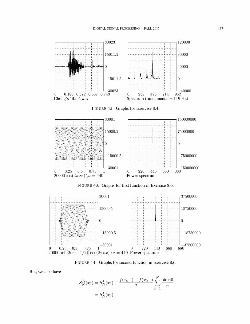
DIGITAL SIGNAL PROCESSING — FALL 2015 137
0 0.186 0.372 0.557 0.743−30023
−15011.5
0
15011.5
30023
Chong’s ’Bait’.wav0 238 476 714 952
−40000
0
40000
80000
120000
Spectrum (fundamental = 119 Hz)
FIGURE 42. Graphs for Exercise 8.4.
0 0.25 0.5 0.75 1−30001
−15000.5
0
15000.5
30001
20000 cos(2πνx) \ν = 4400 220 440 660 880
−150000000
−75000000
0
75000000
150000000
Power spectrum
FIGURE 43. Graphs for first function in Exercise 8.6.
0 0.25 0.5 0.75 1−30001
−15000.5
0
15000.5
30001
20000bell[2(x− 1/2)] cos(2πνx) \ν = 4400 220 440 660 880
−37500000
−18750000
0
18750000
37500000
Power spectrum
FIGURE 44. Graphs for second function in Exercise 8.6.
But, we also have
Sf1N (x0) = Sf
N (x0) +f(x0+) + f(x0−)
2
N∑
n=1
sinn0
n
= SfN (x0).
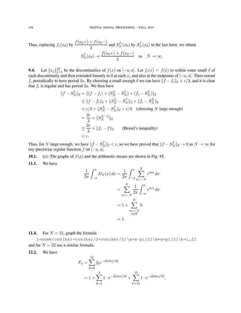
138 DIGITAL SIGNAL PROCESSING — FALL 2015
Thus, replacing f1(x0) byf(x0+) + f(x0−)
2and Sf1
N (x0) by SfN (x0) in the last limit, we obtain
SfN (x0) →
f(x0+) + f(x0−)
2as N → ∞.
9.4. Let xjMj=1 be the discontinuities of f(x) on [−a, a]. Let fǫ(x) = f(x) to within some small δ of
each discontinuity and then extended linearly to 0 at each xj and also at the endpoints of [−a, a]. Then extend
fǫ periodically to have period 2a. By choosing a small enough δ we can have ‖f − fǫ‖2 < ǫ/3, and it is clear
that fǫ is regular and has period 2a. We then have
‖f − SfN‖2 = ‖(f − fǫ) + (Sfǫ
N − SfN ) + (fǫ − Sfǫ
N )‖2≤ ‖f − fǫ‖2 + ‖Sfǫ
N − SfN‖2 + ‖fǫ − Sfǫ
N ‖2< ǫ/3 + ‖Sfǫ
N − SfN‖2 + ǫ/3 (choosing N large enough)
=2ǫ
3+ ‖Sfǫ−f
N ‖2
≤ 2ǫ
3+ ‖fǫ − f‖2 (Bessel’s inequality)
< ǫ.
Thus, for N large enough, we have ‖f − SfN‖2 < ǫ, so we have proved that ‖f − Sf
N‖2 → 0 as N → ∞ for
any piecewise regular function f on [−a, a].
10.1. (c): The graphs of f(x) and the arithmetic means are shown in Fig. 45.
11.1. We have
1
2π
∫ π
−πDN (x) dx =
1
2π
∫ π
−π
N∑
n=−N
einx dx
=
N∑
n=−N
1
2π
∫ π
−πeinx dx
= 1 +
N∑
n=−Nn 6=0
0
= 1.
11.4. For N = 21, graph the formula
1+sumkcos(kx)+cos(ka)/2+cos(kb)/2\a=x-pi/21\b=x+pi/21\k=1,21
and for N = 22 use a similar formula.
12.2. We have
Fn =16∑
k=0
fke−i2πkn/16
= 1 +
4∑
k=1
1 · e−i2πkn/16 +
15∑
k=12
1 · e−i2πkn/16.
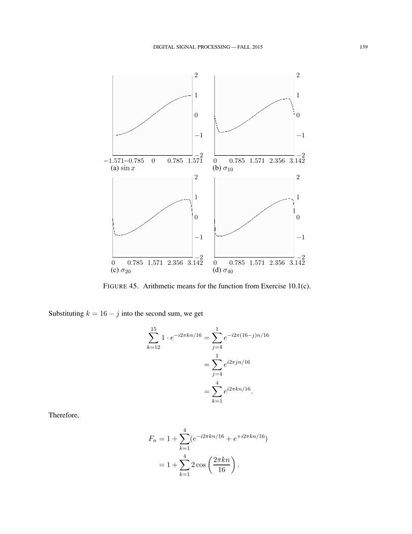
DIGITAL SIGNAL PROCESSING — FALL 2015 139
−1.571−0.785 0 0.785 1.571−2
−1
0
1
2
(a) sinx0 0.785 1.571 2.356 3.142
−2
−1
0
1
2
(b) σ10
0 0.785 1.571 2.356 3.142−2
−1
0
1
2
(c) σ200 0.785 1.571 2.356 3.142
−2
−1
0
1
2
(d) σ40
FIGURE 45. Arithmetic means for the function from Exercise 10.1(c).
Substituting k = 16− j into the second sum, we get
15∑
k=12
1 · e−i2πkn/16 =
1∑
j=4
e−i2π(16−j)n/16
=
1∑
j=4
ei2πjn/16
=4∑
k=1
ei2πkn/16.
Therefore,
Fn = 1 +4∑
k=1
(e−i2πkn/16 + e+i2πkn/16)
= 1 +
4∑
k=1
2 cos
(2πkn
16
).
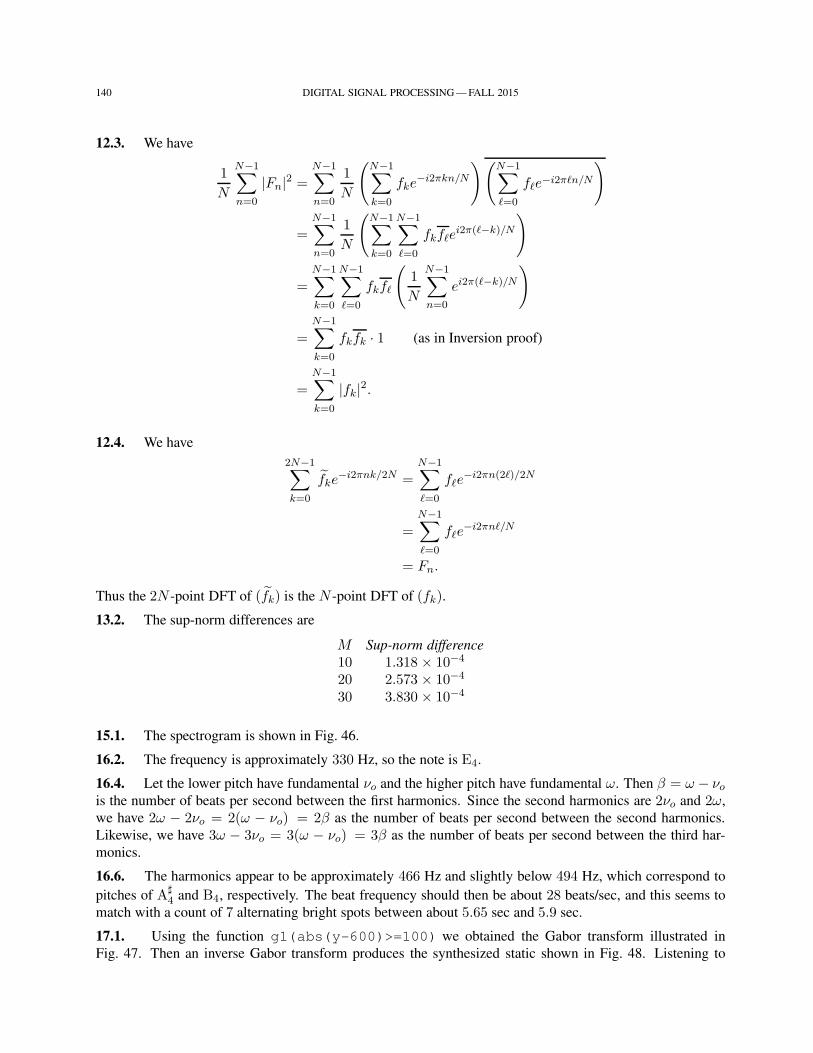
140 DIGITAL SIGNAL PROCESSING — FALL 2015
12.3. We have
1
N
N−1∑
n=0
|Fn|2 =N−1∑
n=0
1
N
(N−1∑
k=0
fke−i2πkn/N
)(N−1∑
ℓ=0
fℓe−i2πℓn/N
)
=N−1∑
n=0
1
N
(N−1∑
k=0
N−1∑
ℓ=0
fkfℓei2π(ℓ−k)/N
)
=
N−1∑
k=0
N−1∑
ℓ=0
fkfℓ
(1
N
N−1∑
n=0
ei2π(ℓ−k)/N
)
=
N−1∑
k=0
fkfk · 1 (as in Inversion proof)
=
N−1∑
k=0
|fk|2.
12.4. We have
2N−1∑
k=0
fke−i2πnk/2N =
N−1∑
ℓ=0
fℓe−i2πn(2ℓ)/2N
=
N−1∑
ℓ=0
fℓe−i2πnℓ/N
= Fn.
Thus the 2N -point DFT of (fk) is the N -point DFT of (fk).
13.2. The sup-norm differences are
M Sup-norm difference
10 1.318 × 10⁻⁴
20 2.573 × 10⁻⁴
30 3.830 × 10⁻⁴
15.1. The spectrogram is shown in Fig. 46.
16.2. The frequency is approximately 330 Hz, so the note is E4.
16.4. Let the lower pitch have fundamental νo and the higher pitch have fundamental ω. Then β = ω − νois the number of beats per second between the first harmonics. Since the second harmonics are 2νo and 2ω,
we have 2ω − 2νo = 2(ω − νo) = 2β as the number of beats per second between the second harmonics.
Likewise, we have 3ω − 3νo = 3(ω − νo) = 3β as the number of beats per second between the third har-
monics.
16.6. The harmonics appear to be approximately 466 Hz and slightly below 494 Hz, which correspond to
pitches of A♯4 and B4, respectively. The beat frequency should then be about 28 beats/sec, and this seems to
match with a count of 7 alternating bright spots between about 5.65 sec and 5.9 sec.
17.1. Using the function g1(abs(y-600)>=100) we obtained the Gabor transform illustrated in
Fig. 47. Then an inverse Gabor transform produces the synthesized static shown in Fig. 48. Listening to
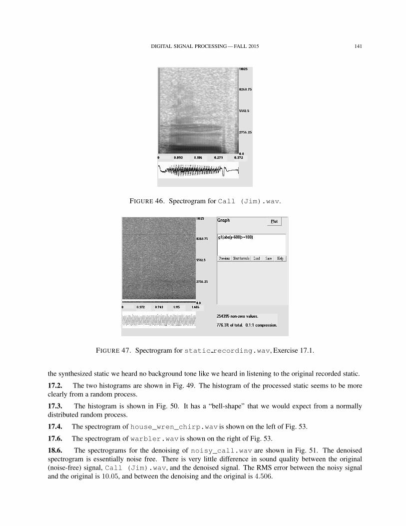
DIGITAL SIGNAL PROCESSING — FALL 2015 141
FIGURE 46. Spectrogram for Call (Jim).wav.
FIGURE 47. Spectrogram for static recording.wav, Exercise 17.1.
the synthesized static we heard no background tone like we heard in listening to the original recorded static.
17.2. The two histograms are shown in Fig. 49. The histogram of the processed static seems to be more
clearly from a random process.
17.3. The histogram is shown in Fig. 50. It has a “bell-shape” that we would expect from a normally
distributed random process.
17.4. The spectrogram of house_wren_chirp.wav is shown on the left of Fig. 53.
17.6. The spectrogram of warbler.wav is shown on the right of Fig. 53.
18.6. The spectrograms for the denoising of noisy_call.wav are shown in Fig. 51. The denoised
spectrogram is essentially noise free. There is very little difference in sound quality between the original
(noise-free) signal, Call (Jim).wav, and the denoised signal. The RMS error between the noisy signal
and the original is 10.05, and between the denoising and the original is 4.506.
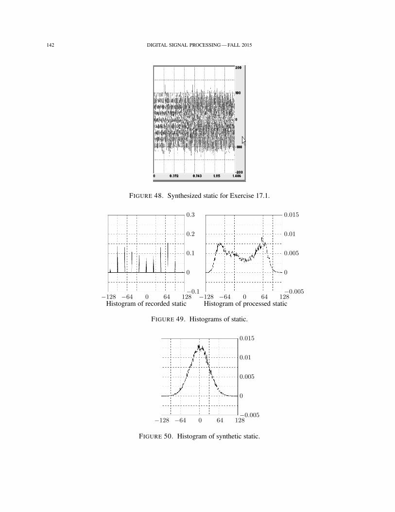
142 DIGITAL SIGNAL PROCESSING — FALL 2015
FIGURE 48. Synthesized static for Exercise 17.1.
−128 −64 0 64 128−0.1
0
0.1
0.2
0.3
Histogram of recorded static−128 −64 0 64 128
−0.005
0
0.005
0.01
0.015
Histogram of processed static
FIGURE 49. Histograms of static.
−128 −64 0 64 128−0.005
0
0.005
0.01
0.015
FIGURE 50. Histogram of synthetic static.
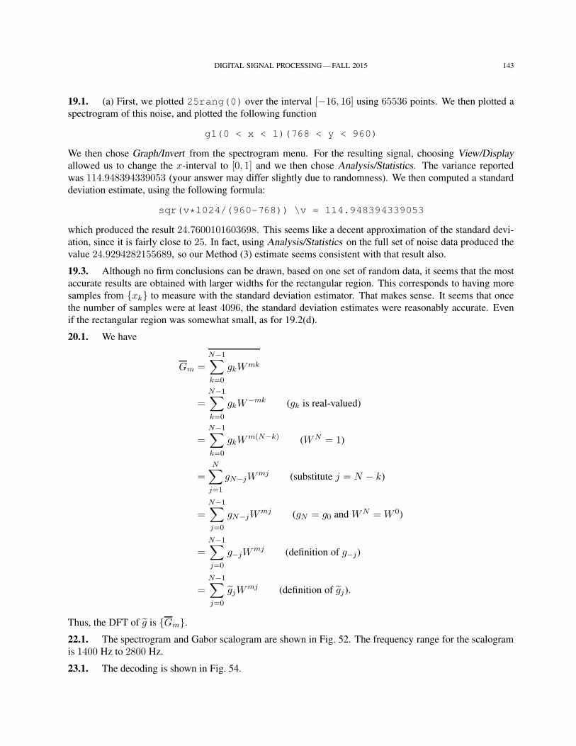
DIGITAL SIGNAL PROCESSING — FALL 2015 143
19.1. (a) First, we plotted 25rang(0) over the interval [−16, 16] using 65536 points. We then plotted a
spectrogram of this noise, and plotted the following function
g1(0 < x < 1)(768 < y < 960)
We then chose Graph/Invert from the spectrogram menu. For the resulting signal, choosing View/Display
allowed us to change the x-interval to [0, 1] and we then chose Analysis/Statistics. The variance reported
was 114.948394339053 (your answer may differ slightly due to randomness). We then computed a standard
deviation estimate, using the following formula:
sqr(v*1024/(960-768)) \v = 114.948394339053
which produced the result 24.7600101603698. This seems like a decent approximation of the standard devi-
ation, since it is fairly close to 25. In fact, using Analysis/Statistics on the full set of noise data produced the
value 24.9294282155689, so our Method (3) estimate seems consistent with that result also.
19.3. Although no firm conclusions can be drawn, based on one set of random data, it seems that the most
accurate results are obtained with larger widths for the rectangular region. This corresponds to having more
samples from xk to measure with the standard deviation estimator. That makes sense. It seems that once
the number of samples were at least 4096, the standard deviation estimates were reasonably accurate. Even
if the rectangular region was somewhat small, as for 19.2(d).
20.1. We have
Gm =
N−1∑
k=0
gkWmk
=N−1∑
k=0
gkW−mk (gk is real-valued)
=
N−1∑
k=0
gkWm(N−k) (WN = 1)
=
N∑
j=1
gN−jWmj (substitute j = N − k)
=N−1∑
j=0
gN−jWmj (gN = g0 and WN = W 0)
=
N−1∑
j=0
g−jWmj (definition of g−j)
=N−1∑
j=0
gjWmj (definition of gj).
Thus, the DFT of g is Gm.22.1. The spectrogram and Gabor scalogram are shown in Fig. 52. The frequency range for the scalogram
is 1400 Hz to 2800 Hz.
23.1. The decoding is shown in Fig. 54.
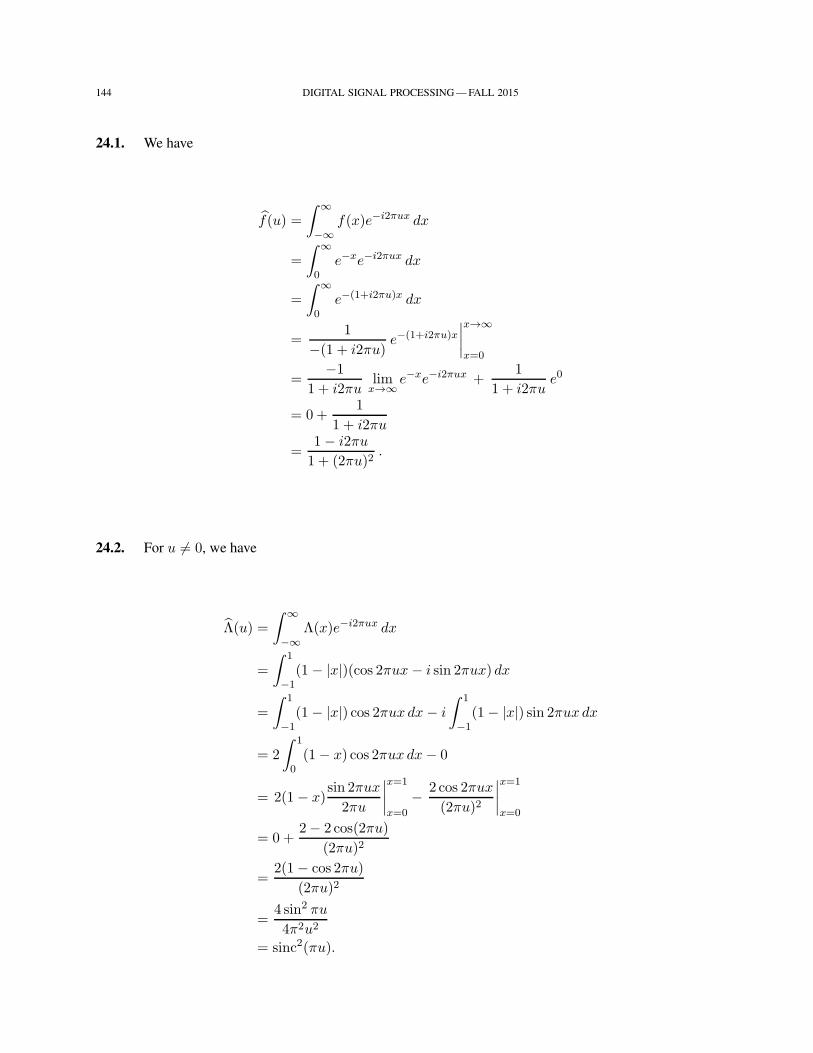
144 DIGITAL SIGNAL PROCESSING — FALL 2015
24.1. We have
f(u) =
∫ ∞
−∞f(x)e−i2πux dx
=
∫ ∞
0e−xe−i2πux dx
=
∫ ∞
0e−(1+i2πu)x dx
=1
−(1 + i2πu)e−(1+i2πu)x
∣∣∣∣x→∞
x=0
=−1
1 + i2πulimx→∞
e−xe−i2πux +1
1 + i2πue0
= 0 +1
1 + i2πu
=1− i2πu
1 + (2πu)2.
24.2. For u 6= 0, we have
Λ(u) =
∫ ∞
−∞Λ(x)e−i2πux dx
=
∫ 1
−1(1− |x|)(cos 2πux− i sin 2πux) dx
=
∫ 1
−1(1− |x|) cos 2πux dx− i
∫ 1
−1(1− |x|) sin 2πux dx
= 2
∫ 1
0(1− x) cos 2πux dx− 0
= 2(1− x)sin 2πux
2πu
∣∣∣∣x=1
x=0
− 2 cos 2πux
(2πu)2
∣∣∣∣x=1
x=0
= 0 +2− 2 cos(2πu)
(2πu)2
=2(1− cos 2πu)
(2πu)2
=4 sin2 πu
4π2u2
= sinc2(πu).
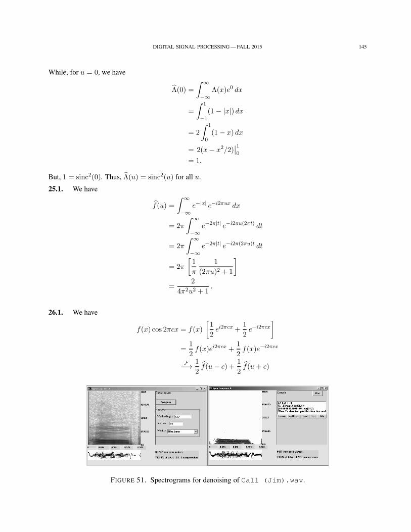
DIGITAL SIGNAL PROCESSING — FALL 2015 145
While, for u = 0, we have
Λ(0) =
∫ ∞
−∞Λ(x)e0 dx
=
∫ 1
−1(1− |x|) dx
= 2
∫ 1
0(1− x) dx
= 2(x− x2/2)∣∣10
= 1.
But, 1 = sinc2(0). Thus, Λ(u) = sinc2(u) for all u.
25.1. We have
f(u) =
∫ ∞
−∞e−|x| e−i2πux dx
= 2π
∫ ∞
−∞e−2π|t| e−i2πu(2πt) dt
= 2π
∫ ∞
−∞e−2π|t| e−i2π(2πu)t dt
= 2π
[1
π
1
(2πu)2 + 1
]
=2
4π2u2 + 1.
26.1. We have
f(x) cos 2πcx = f(x)
[1
2ei2πcx +
1
2e−i2πcx
]
=1
2f(x)ei2πcx +
1
2f(x)e−i2πcx
F−→ 1
2f(u− c) +
1
2f(u+ c)
FIGURE 51. Spectrograms for denoising of Call (Jim).wav.
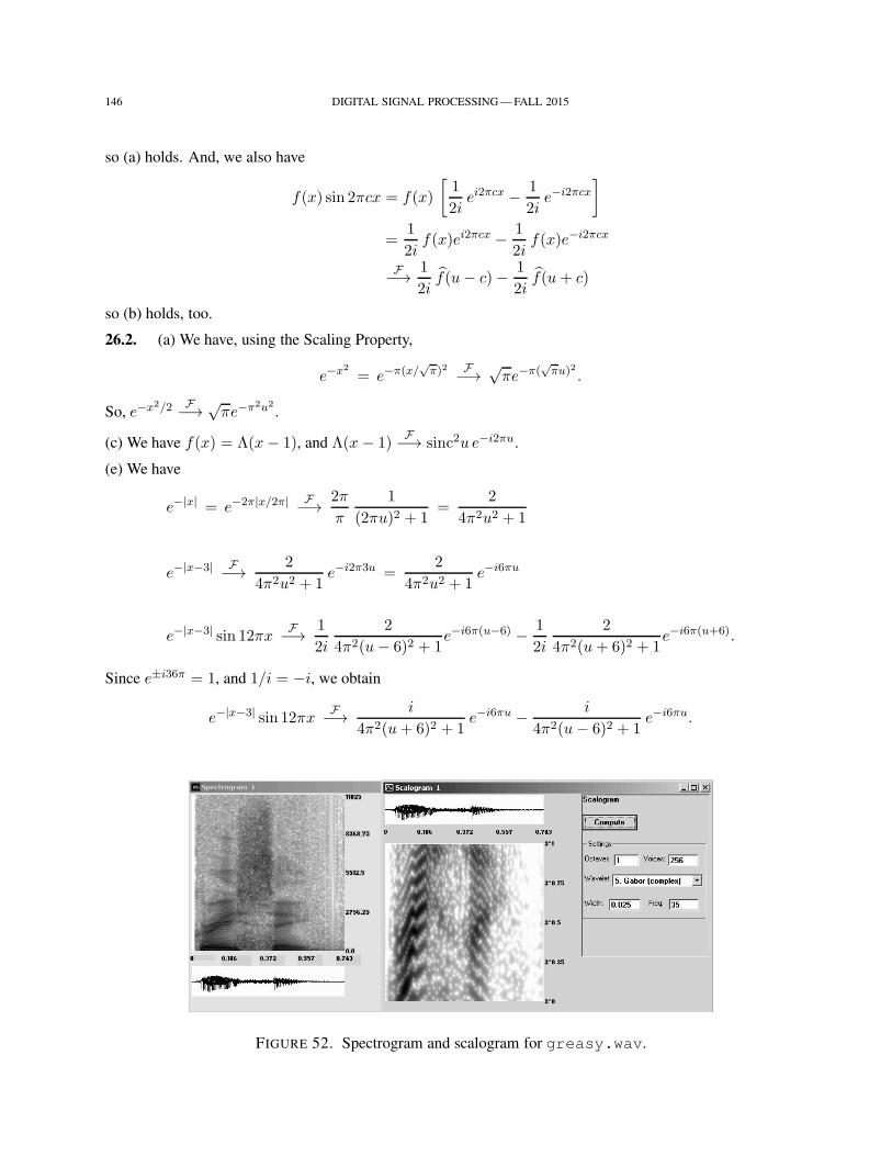
146 DIGITAL SIGNAL PROCESSING — FALL 2015
so (a) holds. And, we also have
f(x) sin 2πcx = f(x)
[1
2iei2πcx − 1
2ie−i2πcx
]
=1
2if(x)ei2πcx − 1
2if(x)e−i2πcx
F−→ 1
2if(u− c)− 1
2if(u+ c)
so (b) holds, too.
26.2. (a) We have, using the Scaling Property,
e−x2= e−π(x/
√π)2 F−→ √
πe−π(√πu)2 .
So, e−x2/2 F−→ √πe−π2u2
.
(c) We have f(x) = Λ(x− 1), and Λ(x− 1)F−→ sinc2u e−i2πu.
(e) We have
e−|x| = e−2π|x/2π| F−→ 2π
π
1
(2πu)2 + 1=
2
4π2u2 + 1
e−|x−3| F−→ 2
4π2u2 + 1e−i2π3u =
2
4π2u2 + 1e−i6πu
e−|x−3| sin 12πxF−→ 1
2i
2
4π2(u− 6)2 + 1e−i6π(u−6) − 1
2i
2
4π2(u+ 6)2 + 1e−i6π(u+6).
Since e±i36π = 1, and 1/i = −i, we obtain
e−|x−3| sin 12πxF−→ i
4π2(u+ 6)2 + 1e−i6πu − i
4π2(u− 6)2 + 1e−i6πu.
FIGURE 52. Spectrogram and scalogram for greasy.wav.
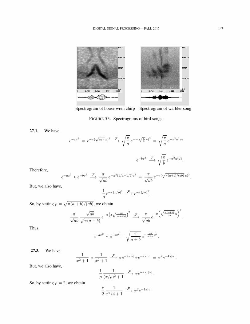
DIGITAL SIGNAL PROCESSING — FALL 2015 147
Spectrogram of house wren chirp Spectrogram of warbler song
FIGURE 53. Spectrograms of bird songs.
27.1. We have
e−ax2= e−π(
√a/π x)2 F−→
√π
ae−π(
√πau)2 =
√π
ae−π2u2/a
e−bx2 F−→√
π
be−π2u2/b.
Therefore,
e−ax2 ∗ e−bx2 F−→ π√ab
e−π2(1/a+1/b)u2=
π√ab
e−π(√
π(a+b)/(ab) u)2 .
But, we also have,1
ρe−π(x/ρ)2 F−→ e−π(ρu)2 .
So, by setting ρ =√
π(a+ b)/(ab), we obtain
π√ab
√ab√
π(a+ b)e−π
(x√
abπ(a+b)
)2F−→ π√
abe−π
(√π(a+b)
abu
)2
.
Thus,
e−ax2 ∗ e−bx2=
√π
a+ be−
aba+b
x2
.
27.3. We have1
x2 + 1∗ 1
x2 + 1
F−→ πe−2π|u| πe−2π|u| = π2e−4π|u|.
But, we also have,1
ρ
1
(x/ρ)2 + 1
F−→ πe−2πρ|u|.
So, by setting ρ = 2, we obtainπ
2
1
x2/4 + 1F−→ π2e−4π|u|
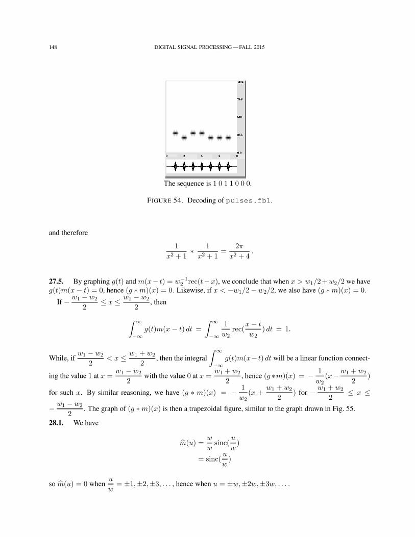
148 DIGITAL SIGNAL PROCESSING — FALL 2015
The sequence is 1 0 1 1 0 0 0.
FIGURE 54. Decoding of pulses.fb1.
and therefore
1
x2 + 1∗ 1
x2 + 1=
2π
x2 + 4.
27.5. By graphing g(t) and m(x− t) = w−12 rec(t−x), we conclude that when x > w1/2+w2/2 we have
g(t)m(x− t) = 0, hence (g ∗m)(x) = 0. Likewise, if x < −w1/2− w2/2, we also have (g ∗m)(x) = 0.
If − w1 − w2
2≤ x ≤ w1 − w2
2, then
∫ ∞
−∞g(t)m(x − t) dt =
∫ ∞
−∞
1
w2rec(
x− t
w2) dt = 1.
While, ifw1 − w2
2< x ≤ w1 + w2
2, then the integral
∫ ∞
−∞g(t)m(x− t) dt will be a linear function connect-
ing the value 1 at x =w1 − w2
2with the value 0 at x =
w1 + w2
2, hence (g ∗m)(x) = − 1
w2(x− w1 + w2
2)
for such x. By similar reasoning, we have (g ∗ m)(x) = − 1
w2(x +
w1 + w2
2) for − w1 +w2
2≤ x ≤
− w1 −w2
2. The graph of (g ∗m)(x) is then a trapezoidal figure, similar to the graph drawn in Fig. 55.
28.1. We have
m(u) =w
wsinc(
u
w)
= sinc(u
w)
so m(u) = 0 whenu
w= ±1,±2,±3, . . . , hence when u = ±w,±2w,±3w, . . . .
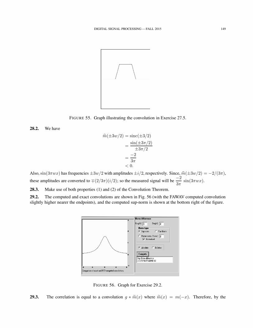
DIGITAL SIGNAL PROCESSING — FALL 2015 149
FIGURE 55. Graph illustrating the convolution in Exercise 27.5.
28.2. We have
m(±3w/2) = sinc(±3/2)
=sin(±3π/2)
±3π/2
=−2
3π< 0.
Also, sin(3πwx) has frequencies ±3w/2 with amplitudes ±i/2, respectively. Since, m(±3w/2) = −2/(3π),
these amplitudes are converted to ∓(2/3π)(i/2); so the measured signal will be−2
3πsin(3πwx).
28.3. Make use of both properties (1) and (2) of the Convolution Theorem.
29.2. The computed and exact convolutions are shown in Fig. 56 (with the FAWAV computed convolution
slightly higher nearer the endpoints), and the computed sup-norm is shown at the bottom right of the figure.
FIGURE 56. Graph for Exercise 29.2.
29.3. The correlation is equal to a convolution g ∗ m(x) where m(x) = m(−x). Therefore, by the
150 DIGITAL SIGNAL PROCESSING — FALL 2015
Convolution Theorem
g ∗ m F−→ g(u) m(u).
And, we also have
m(u) =
∫ ∞
−∞m(−x)e−i2πux dx
=
∫ −∞
∞m(t)ei2πut (−dt)
=
∫ ∞
−∞m(t)ei2πut dt
(m is real) =
∫ ∞
−∞m(t)e−i2πut dt
= m(u) .
Thus, the Fourier transform of the correlation is g(u)m(u).We have thus shown that
g,m → g, m F−→ g, m → gm F−1
−→ g ∗ m.
This is discretized as
g(xk),m(xk) → g(xk), m(xk) FFT−→ Gn,Mn → GnMn FFT−1
−→ g ∗ m(xk).
30.3. Since ei2πu(1/2) = eiπu = cosπu+ i sinπu, we have
sinc u ei2πu(1/2) =sinπu
πucos πu+ i
sinπu
πusinπu.
Sincesinπu
πusinπu is an odd function, and
sinπu
πucos πu is an even function, we obtain
∫ L
−Lsincu ei2πu(1/2) du = 2
∫ L
0
sinπu
πucosπu du
=
∫ L
0
sin 2πu
πudu.
So, we have
limL→∞
∫ L
−Lsincu ei2πu(1/2) du =
∫ ∞
0
sin 2πu
πudu
= I(0).
30.4. We have
I ′(α) =d
dα
∫ ∞
0e−αu sin 2πu
πudu
=
∫ ∞
0
∂
∂α
(e−αu sin 2πu
πu
)du
=
∫ ∞
0
−e−αu sin 2πu
πdu.
DIGITAL SIGNAL PROCESSING — FALL 2015 151
Integrating by parts twice, we have∫ ∞
0
−e−αu sin 2πu
πdu =
cos 2πu
2π2e−αu
∣∣∣∣∞
0
+α
4π3e−αu sin 2πu
∣∣∣∞
0+
α2
4π3
∫ ∞
0e−αu sin 2πu du
=−1
2π2+
α2
4π3
∫ ∞
0e−αu sin 2πu du.
Therefore, (1 +
α2
4π2
) (∫ ∞
0
−e−αu sin 2πu
πdu
)=
−1
2π2
and that gives
I ′(α) =−1/2π2
1 + α2/4π2
=−1
π
1/2π
1 + (α/2π)2.
Integrating this last equation, we get
I(α) = C − 1
πtan−1
( α
2π
).
Since I(α) → 0 as α → ∞, we must have C = 1/2. Thus,
I(α) =1
2− 1
πtan−1
( α
2π
).
Putting α = 0, we get I(0) = 1/2.
30.5. The value of C insures that g(x0−) = f(x0+) = g(x0+). Hence, g has a removable discontinuity at
x0. Therefore, we may define g(x0) = f(x0+), and thereby assume that g is continuous at x0. Consequently,
by the proof for points of continuity given in the text, we have
limL→∞
SgL(x0) = g(x0) = f(x0+)
where
SgL(x0) =
∫ L
−Lg(u) ei2πux0 du
=
∫ L
−Lf(u) ei2πux0du+
∫ L
−LC sincu e−i2π(x0−1/2) ei2πux0 du
= SfL(x0) + C
∫ L
−Lsincu eiπu du.
By the solution to Exercise 30.4, we have
limL→∞
C
∫ L
−Lsinc u eiπu du =
1
2C
=1
2(f(x0+)− f(x0−)) .
Therefore, we obtain
limL→∞
SfL(x0) = g(x0)−
1
2(f(x0+)− f(x0−))
=1
2(f(x0+) + f(x0−)) .
152 DIGITAL SIGNAL PROCESSING — FALL 2015
That completes the proof of the inversion theorem, since we have proved the theorem for a jump discontinuity
at x0.
31.1. We have f(x) = sinc2(4(x − 3/4)), and we know that sinc2(4x)F−→ Λ(u/4)/4, and that gives us
f(u) =1
4Λ(u4
)e−i2π(3/4)u.
Since e−i2π(3/4)u 6= 0 for any u, it follows that f(u) = 0 only when Λ(u/4) = 0. Graphing Λ(u/4) we see
that it is 0 precisely when u is outside of the open interval (−4, 4). Consequently, L = 4.
31.2. The reconstruction series is
f(x) =∞∑
n=−∞sinc2 (4(n/8)− 3) sinc(8x− n).
32.1. We have
3sinc2(4x− 2) = 3sinc2(4(x− 1/2))
so f(u) = 0.75Λ(u/4) e−i2π(1/2)u . Therefore, LN
= 4, and the Nyquist series is
∞∑
n=−∞3 sinc2 (4(n/8) − 2) sinc(8x− n).
The graphs of f(x) and SM for M = 16, 32, 64 are shown in Fig. 57, and the sup-norms are shown in Table 3.
TABLE 3. SUP-NORM DIFFERENCES FOR EXERCISE 32.1
M ‖f − SM‖sup16 2.668 × 10⁻³
32 1.108 × 10⁻⁴
64 1.206 × 10⁻⁵
34.1. (a) fe(x) = rec(x+ 2) + rec(x− 2), so
FC[f ](u) = F [fe](u)
= sinc(u)ei2π·2u + sinc(u)e−i2π·2u
= 2 sinc(u) cos(4πu).
. (c) fe(x) = e−4πx2, so
FC[f ](u) = F [e−4πx2](u)
=1
2e−πu2/4.
34.3. The graphs of the original data and the double cosine-transformed data appear to be identical random
data. We found a Sup-norm difference of 8.3149×10⁻¹² . Your results may differ slightly, due to randomness
of the data, but should also show a negligible Sup-norm difference.
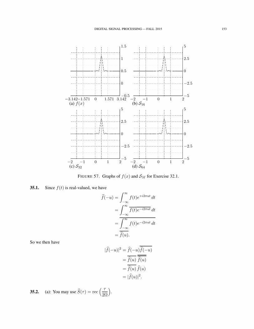
DIGITAL SIGNAL PROCESSING — FALL 2015 153
−3.142−1.571 0 1.571 3.142−0.5
0
0.5
1
1.5
(a) f(x)−2 −1 0 1 2
−5
−2.5
0
2.5
5
(b) S16
−2 −1 0 1 2−5
−2.5
0
2.5
5
(c) S32
−2 −1 0 1 2−5
−2.5
0
2.5
5
(d) S64
FIGURE 57. Graphs of f(x) and SM for Exercise 32.1.
35.1. Since f(t) is real-valued, we have
f(−u) =
∫ ∞
−∞f(t)e+i2πut dt
=
∫ ∞
−∞f(t)e−i2πut dt
=
∫ ∞
−∞f(t)e−i2πut dt
= f(u).
So we then have
|f(−u)|2 = f(−u)f(−u)
= f(u) f(u)
= f(u) f(u)
= |f(u)|2.
35.2. (a): You may use S(τ) = rec( τ
2Ω
).


![ECE-V-DIGITAL SIGNAL PROCESSING [10EC52] …vtusolution.in/.../digital-signal-processing-10ec52.pdfDigital vtusolution.in Signal Processing 10EC52 TEXT BOOK: 1. DIGITAL SIGNAL PROCESSING](https://img.pdfslide.us/doc/110x75/5afe42bb7f8b9a256b8ccd2e/ece-v-digital-signal-processing-10ec52-signal-processing-10ec52-text-book.jpg)