Embed Size (px)
Citation preview
1 DEPT OF ECE
DIGITAL SIGNAL PROCESSING
LAB MANUAL
Subject Code : A60493
Regulations : R15 – JNTUH
Class : III Year II Semester (ECE)
Mrs .C. Devi supraja
Assistant Professor
Department of Electronics & Communication Engineering
INSTITUTE OF AERONAUTICAL ENGINEERING (Autonomous)
Dundigal – 500 043, Hyderabad
Prepared by Dr. Prashant Pradhan
Professor
Mrs. G. Mary
Swarnalatha
Assistant Professor
Mr.V Naresh Kumar
Assistant Professor

2 DEPT OF ECE
INSTITUTE OF AERONAUTICAL ENGINEERING (Autonomous)
Dundigal - 500 043, Hyderabad
Electronics & Communication Engineering
Vision
To produce professionally competent Electronics and Communication Engineers capable of
effectively and efficiently addressing the technical challenges with social responsibility.
Mission The mission of the Department is to provide an academic environment that will ensure high
quality education, training and research by keeping the students abreast of latest developments in
the field of Electronics and Communication Engineering aimed at promoting employability,
leadership qualities with humanity, ethics, research aptitude and team spirit.
Quality Policy Our policy is to nurture and build diligent and dedicated community of engineers providing a
professional and unprejudiced environment, thus justifying the purpose of teaching and
satisfying the stake holders.
A team of well qualified and experienced professionals ensure quality education with its
practical application in all areas of the Institute.
Philosophy The essence of learning lies in pursuing the truth that liberates one from the darkness of
ignorance and Institute of Aeronautical Engineering firmly believes that education is for
liberation.
Contained therein is the notion that engineering education includes all fields of science that plays
a pivotal role in the development of world-wide community contributing to the progress of
civilization. This institute, adhering to the above understanding, is committed to the development
of science and technology in congruence with the natural environs. It lays great emphasis on
intensive research and education that blends professional skills and high moral standards with a
sense of individuality and humanity. We thus promote ties with local communities and
encourage transnational interactions in order to be socially accountable. This accelerates the
process of transfiguring the students into complete human beings making the learning process
relevant to life, instilling in them a sense of courtesy and responsibility.

3 DEPT OF ECE
INSTITUTE OF AERONAUTICAL ENGINEERING (Autonomous)
Dundigal, Hyderabad - 500 043
Electronics & Communication Engineering
Program Outcomes
PO1 Apply the knowledge of mathematics, science, engineering fundamentals, and an engineering
specialization to the solution of complex engineering problems.
PO2
Identify, formulate, review research literature, and analyze complex engineering problems reaching
substantiated conclusions using first principles of mathematics, natural sciences, and engineering
sciences.
PO3
Design solutions for complex engineering problems and design system components or processes that
meet the specified needs with appropriate consideration for the public health and safety, and the
cultural, societal, and environmental considerations.
PO4 Use research-based knowledge and research methods including design of experiments, analysis and
interpretation of data, and synthesis of the information to provide valid conclusions.
PO5
Create, select, and apply appropriate techniques, resources, and modern engineering and IT tools
including prediction and modelling to complex engineering activities with an understanding of the
limitations.
PO6 Apply reasoning informed by the contextual knowledge to assess societal, health, safety, legal and
cultural issues and the consequent responsibilities relevant to the professional engineering practice.
PO7 Understand the impact of the professional engineering solutions in societal and environmental contexts,
and demonstrate the knowledge of, and need for sustainable development.
PO8 Apply ethical principles and commit to professional ethics and responsibilities and norms of the
engineering practice.
PO9 Function effectively as an individual, and as a member or leader in diverse teams, and in
multidisciplinary settings.
PO10
Communicate effectively on complex engineering activities with the engineering community and with
society at large, such as, being able to comprehend and write effective reports and design
documentation, make effective presentations, and give and receive clear instructions.
PO11
Demonstrate knowledge and understanding of the engineering and management principles and apply
these to one‟s own work, as a member and leader in a team, to manage projects and in multidisciplinary
environments.
PO12 Recognize the need for, and have the preparation and ability to engage in independent and life-long
learning in the broadest context of technological change.
Program Specific Outcomes
PSO1
Professional Skills:An ability to understand the basic concepts in Electronics & Communication
Engineering and to apply them to various areas, like Electronics, Communications, Signal processing,
VLSI, Embedded systems etc., in the design and implementation of complex systems.
PSO2
Problem-solving skills:An ability to solve complex Electronics and communication Engineering
problems, using latest hardware and software tools, along with analytical skills to arrive cost effective
and appropriate solutions.
PSO3
Successful career and Entrepreneurship:An understanding of social-awareness & environmental-
wisdom along with ethical responsibility to have a successful career and to sustain passion and zeal for
real-world applications using optimal resources as an Entrepreneur.
4 DEPT OF ECE
INSTITUTE OF AERONAUTICAL ENGINEERING (Autonomous)
Dundigal, Hyderabad - 500 043
Electronics & Communication Engineering
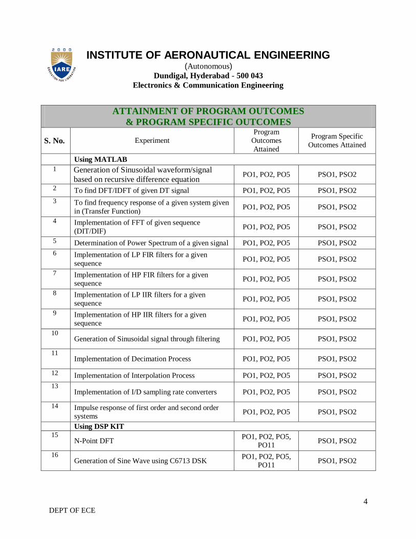
ATTAINMENT OF PROGRAM OUTCOMES
& PROGRAM SPECIFIC OUTCOMES
S. No. Experiment Program
Outcomes
Attained
Program Specific
Outcomes Attained
Using MATLAB
1 Generation of Sinusoidal waveform/signal
based on recursive difference equation PO1, PO2, PO5 PSO1, PSO2
2 To find DFT/IDFT of given DT signal PO1, PO2, PO5 PSO1, PSO2
3 To find frequency response of a given system given
in (Transfer Function) PO1, PO2, PO5 PSO1, PSO2
4 Implementation of FFT of given sequence
(DIT/DIF) PO1, PO2, PO5 PSO1, PSO2
5 Determination of Power Spectrum of a given signal PO1, PO2, PO5 PSO1, PSO2
6 Implementation of LP FIR filters for a given
sequence PO1, PO2, PO5 PSO1, PSO2
7 Implementation of HP FIR filters for a given sequence
PO1, PO2, PO5 PSO1, PSO2
8 Implementation of LP IIR filters for a given sequence
PO1, PO2, PO5 PSO1, PSO2
9 Implementation of HP IIR filters for a given sequence
PO1, PO2, PO5 PSO1, PSO2
10 Generation of Sinusoidal signal through filtering PO1, PO2, PO5 PSO1, PSO2
11 Implementation of Decimation Process PO1, PO2, PO5 PSO1, PSO2
12 Implementation of Interpolation Process PO1, PO2, PO5 PSO1, PSO2
13 Implementation of I/D sampling rate converters PO1, PO2, PO5 PSO1, PSO2
14 Impulse response of first order and second order systems
PO1, PO2, PO5 PSO1, PSO2
Using DSP KIT 15
N-Point DFT PO1, PO2, PO5,
PO11 PSO1, PSO2
16 Generation of Sine Wave using C6713 DSK
PO1, PO2, PO5, PO11
PSO1, PSO2
5 DEPT OF ECE
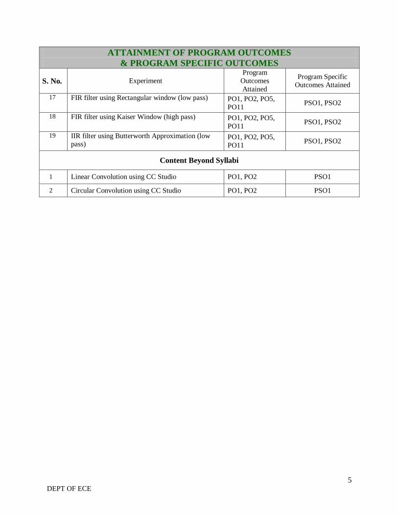
ATTAINMENT OF PROGRAM OUTCOMES
& PROGRAM SPECIFIC OUTCOMES
S. No. Experiment
Program
Outcomes
Attained
Program Specific Outcomes Attained
17 FIR filter using Rectangular window (low pass) PO1, PO2, PO5,
PO11 PSO1, PSO2
18 FIR filter using Kaiser Window (high pass) PO1, PO2, PO5,
PO11 PSO1, PSO2
19 IIR filter using Butterworth Approximation (low pass)
PO1, PO2, PO5,
PO11 PSO1, PSO2
Content Beyond Syllabi
1 Linear Convolution using CC Studio PO1, PO2 PSO1
2 Circular Convolution using CC Studio PO1, PO2 PSO1

6 DEPT OF ECE
INSTITUTE OF AERONAUTICAL ENGINEERING (Autonomous)
Dundigal, Hyderabad - 500 043
CCeerrttiiffiiccaattee
This is to Certify that it is a bonafied record of Practical work done by
Sri/Kum. _____________________________________ bearing
the Roll No. ______________________ of ____________ Class
_______________________________________ Branch in the
____________________________ laboratory during the Academic
year ___________________ under our supervision.
Head of the Department Lecture In-Charge
External Examiner
Internal Examiner

7 DEPT OF ECE
INSTITUTE OF AERONAUTICAL ENGINEERING (Autonomous)
Dundigal - 500 043, Hyderabad
Electronics & Communication Engineering
DIGITAL SIGNAL PROCESSING LABORATORY
Course Overview:
This laboratory course builds on the lecture course "Digital Signal Processing" which is mandatory for all
students of electronics and communication engineering. This course is devoted to the application of
digital signal processing techniques to implement various types of signal filtering, including FIR and IIR
filters.And use the Fast Fourier Transform in a variety of applications. Students gain experience in how
such digital processes are implemented in practice using MATLAB and also study a standard DSP
platform.
Course Out Comes:
1. Analyze signals using the discrete Fourier transform (DFT).
2. Understand the implementation of FFT algorithm for efficient computation of the DFT.
3. Design digital IIR filters by designing prototypical analog filters and then applying analog to
digital conversion techniques such as the bilinear transformation.
4. Design digital FIR filters using the window method. 5. Alter the sampling rate of a signal using decimation and interpolation.

8 DEPT OF ECE
INSTITUTE OF AERONAUTICAL ENGINEERING (Autonomous)
Dundigal, Hyderabad - 500 043
Electronics & Communication Engineering
INSTRUCTIONS TO THE STUDENTS
1. Students are required to attend all labs.
2. Students should work individually in the hardware and software laboratories.
3. Students have to bring the lab manual cum observation book, record etc along
with them whenever they come for lab work.
4. Should take only the lab manual, calculator (if needed) and a pen or pencil to the
work area.
5. Should learn the prelab questions. Read through the lab experiment to familiarize
themselves with the components and assembly sequence.
6. Should utilize 3 hour‟s time properly to perform the experiment and to record the
readings. Do the calculations, draw the graphs and take signature from the
instructor.
7. If the experiment is not completed in the stipulated time, the pending work has to
be carried out in the leisure hours or extended hours.
8. Should submit the completed record book according to the deadlines set up by the
instructor.
9. For practical subjects there shall be a continuous evaluation during the semester
for 25 sessional marks and 50 end examination marks.
10. Out of 25 internal marks, 15 marks shall be awarded for day-to-day work and 10
marks to be awarded by conducting an internal laboratory test.
9 DEPT OF ECE
INSTITUTE OF AERONAUTICAL ENGINEERING (Autonomous)
Dundigal - 500 043, Hyderabad
Electronics & Communication Engineering
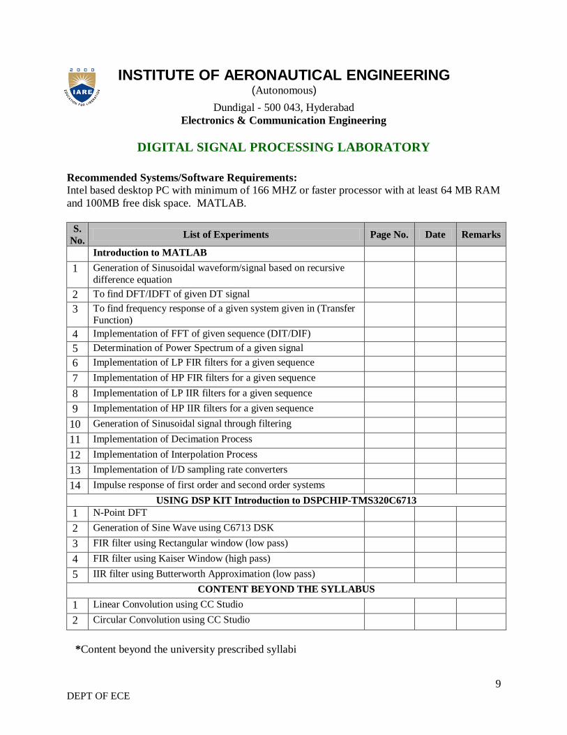
DIGITAL SIGNAL PROCESSING LABORATORY
Recommended Systems/Software Requirements:
Intel based desktop PC with minimum of 166 MHZ or faster processor with at least 64 MB RAM
and 100MB free disk space. MATLAB.
S.
No. List of Experiments Page No. Date Remarks
Introduction to MATLAB
1 Generation of Sinusoidal waveform/signal based on recursive
difference equation
2 To find DFT/IDFT of given DT signal
3 To find frequency response of a given system given in (Transfer
Function)
4 Implementation of FFT of given sequence (DIT/DIF)
5 Determination of Power Spectrum of a given signal
6 Implementation of LP FIR filters for a given sequence
7 Implementation of HP FIR filters for a given sequence
8 Implementation of LP IIR filters for a given sequence
9 Implementation of HP IIR filters for a given sequence
10 Generation of Sinusoidal signal through filtering
11 Implementation of Decimation Process
12 Implementation of Interpolation Process
13 Implementation of I/D sampling rate converters
14 Impulse response of first order and second order systems
USING DSP KIT Introduction to DSPCHIP-TMS320C6713
1 N-Point DFT
2 Generation of Sine Wave using C6713 DSK
3 FIR filter using Rectangular window (low pass)
4 FIR filter using Kaiser Window (high pass)
5 IIR filter using Butterworth Approximation (low pass)
CONTENT BEYOND THE SYLLABUS
1 Linear Convolution using CC Studio
2 Circular Convolution using CC Studio
*Content beyond the university prescribed syllabi
10 DEPT OF ECE
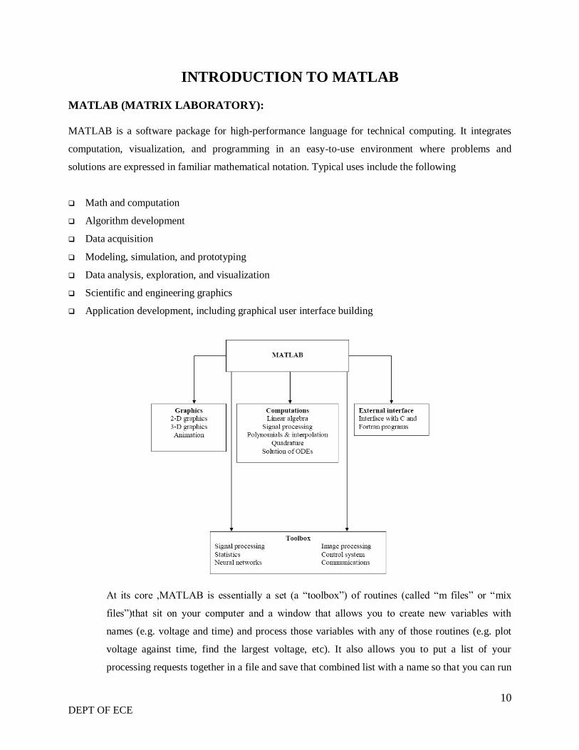
INTRODUCTION TO MATLAB
MATLAB (MATRIX LABORATORY):
MATLAB is a software package for high-performance language for technical computing. It integrates
computation, visualization, and programming in an easy-to-use environment where problems and
solutions are expressed in familiar mathematical notation. Typical uses include the following
Math and computation
Algorithm development
Data acquisition
Modeling, simulation, and prototyping
Data analysis, exploration, and visualization
Scientific and engineering graphics
Application development, including graphical user interface building
At its core ,MATLAB is essentially a set (a “toolbox”) of routines (called “m files” or “mix
files”)that sit on your computer and a window that allows you to create new variables with
names (e.g. voltage and time) and process those variables with any of those routines (e.g. plot
voltage against time, find the largest voltage, etc). It also allows you to put a list of your
processing requests together in a file and save that combined list with a name so that you can run
11 DEPT OF ECE
all of those commands in the same order at some later time. Furthermore, it allows you to run
such lists of commands such that you pass in data and/or get data back out (i.e. the list of
commands is like a function in most programming languages). Once you save a function, it
becomes part of your toolbox (i.e. it now looks to you as if it were part of the basic toolbox that
you started with). For those with computer programming backgrounds: Note that MATLAB runs
as an interpretive language (like the old BASIC). That is, it does not need to be compiled. It
simply reads through each line of the function, executes it, and then goes on to the next line. (In
practice, a form of compilation occurs when you first run a function, so that it can run faster the
next time you run it.)
The name MATLAB stands for matrix laboratory. MATLAB was originally written to provide
easy access to matrix software developed by the LINPACK and EISPACK projects. Today,
MATLAB engines incorporate the LAPACK and BLAS libraries, embedding the state of the art
in software for matrix computation. MATLAB has evolved over a period of years with input
from many users. In university environments, it is the standard instructional tool for introductory
and advanced courses in mathematics, engineering, and science. In industry, MATLAB is the
tool of choice for high-productivity research, development, and analysis.
MATLAB features a family of add-on application-specific solutions called toolboxes. Very
important to most users of MATLAB, toolboxes allow learning and applying specialized
technology. Toolboxes are comprehensive collections of MATLAB functions (M-files) that
extend the MATLAB environment to solve particular classes of problems. Areas in which
toolboxes are available include Image processing, signal processing, control systems, neural
networks, fuzzy logic, wavelets, simulation, and many others.
The main features of MATLAB
Advance algorithm for high performance numerical computation, especially in the Field
matrix algebra
A large collection of predefined mathematical functions and the ability to define one‟s own
functions.
Two-and three dimensional graphics for plotting and displaying data
A complete online help system
Powerful, matrix or vector oriented high level programming language for individual
applications.
12 DEPT OF ECE
Toolboxes available for solving advanced problems in several application areas
MATLAB Windows:
MATLAB works with through three basic windows
COMMAND WINDOW:
This is the main window .it is characterized by MATLAB command prompt >> when you
launch the application program MATLAB puts you in this window all commands including
those for user-written programs ,are typed in this window at the MATLAB prompt
GRAPHICS WINDOW:
the output of all graphics commands typed in the command window are flushed to the graphics
or figure window, a separate gray window with white background color the user can create as
many windows as the system memory will allow
EDIT WINDOW:
This is where you write edit, create and save your own programs in files called M files.
INPUT-OUTPUT:
MATLAB supports interactive computation taking the input from the screen and flushing, the
output to the screen. In addition it can read input files and write output files
DATA TYPE:
The fundamental data –type in MATLAB is the array. It encompasses several distinct data
objects- integers, real numbers, matrices, character strings, structures and cells. There is no need
to declare variables as real or complex, MATLAB automatically sets the variable to be real.
DIMENSIONING:
Dimensioning is automatic in MATLAB. No dimension statements are required for vectors or
arrays .we can find the dimensions of an existing matrix or a vector with the size and length
commands.
The functional unit of data in any MATLAB program is the array. An array is acollection of data
values organized into rows and columns, and known by a single name.MATLAB variable is a
region of memory containing an array, which is known by a userspecifiedname. MATLAB
13 DEPT OF ECE
variable names must begin with a letter, followed by anycombination of letters, numbers, and the
underscore( _ ) character. Only the first 31characters are significant; if more than 31 are used,
the remaining characters will beignored. If two variables are declared with names that only differ
in the 32nd character,MATLAB will treat them as same variable.
Spaces cannot be used in MATLAB variable names, underscore letters can be substitutedto
create meaningful names.It is important to include a data dictionary in the header of any program
that you write. Adata dictionary lists the definition of each variable used in a program. The
definitionshould include both a description of the contents of the item and the units in which it
ismeasured.
MATLAB language is case-sensitive. It is customary to use lower-case letters forordinary
variable names.The most common types of MATLAB variables are double and char.MATLAB
is weakly typed language. Variables are not declared in a program before it isused.
MATLAB variables are created automatically when they are initialized. There are threecommon
ways to initialize variables in MATLAB:
- Assign data to the variable in an assignment system.
- Input data into the variable from the keyboard.
- Read data from a file.
The semicolon at the end of each assignment statement suppresses the automatic echoingof
values that normally occurs whenever an expression is evaluated in an assignmentstatement.
HOW TO INVOKE MATLAB?
Double Click on the MATLAB icon on the desktop.
You will find a Command window where in which you can type the commands and see
theoutput. For example if you type PWD in the command window, it will print current
workingdirectory.
If you want to create a directory type mkdirmydirin the command window, It will create
adirectory called pes.
If you want delete a directory type rmdirmydirin the command window.
HOW TO OPEN A FILE IN MATLAB?
14 DEPT OF ECE
Go to File ->New->M-File and click
Then type the program in the file and save the file with an extension of .m. While giving
filename we should make sure that given file name should not be a command. It is better to the
file name as myconvlution.
HOW TO RUN A MATLAB FILE?
Go to Debug->run and click
Where to work in MATLAB?
All programs and commands can be entered either in the a)Command window b) As an M file
using Mat lab editor Note: Save all M files in the folder 'work' in the current directory.
Otherwise you have to locate the file during compiling. Typing quit in the command prompt>>
quit, will close MATLAB Mat lab Development Environment. For any clarification regarding
plot etc, which are built in functions type help topic i.e. help plot
BASIC INSTRUCTIONS IN MAT LAB
T = 0: 1:10 This instruction indicates a vector T which as initial value 0 and final value 10
with an increment of 1 Therefore T = [0 1 2 3 4 5 6 7 8 9 10]
F= 20: 1: 100 Therefore F = [20 21 22 23 24 ……… 100]
T= 0:1/pi: 1 Therefore T= [0, 0.3183, 0.6366, 0.9549]
zeros (1, 3) The above instruction creates a vector of one row and three columns whose
values are zero Output= [0 0 0]
zeros( 2,4) Output = 0 0 0 0 0 0 0 0
ones (5,2) instruction creates a vector of five rows and two columns
Output = 1 1
1 1
1 1
1 1
a = [ 1 2 3] b = [4 5 6]
o a.*b = [4 10 18]
8 if c= [2 2 2]
o b.*c results in [8 10 12]
15 DEPT OF ECE
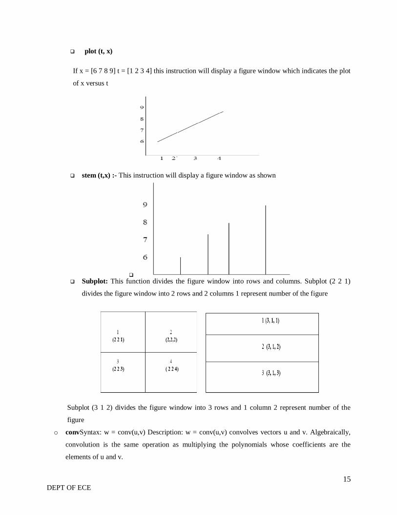
plot (t, x)
If x = [6 7 8 9] t = [1 2 3 4] this instruction will display a figure window which indicates the plot
of x versus t
stem (t,x) :- This instruction will display a figure window as shown
Subplot: This function divides the figure window into rows and columns. Subplot (2 2 1)
divides the figure window into 2 rows and 2 columns 1 represent number of the figure
Subplot (3 1 2) divides the figure window into 3 rows and 1 column 2 represent number of the
figure
o convSyntax: w = conv(u,v) Description: w = conv(u,v) convolves vectors u and v. Algebraically,
convolution is the same operation as multiplying the polynomials whose coefficients are the
elements of u and v.
16 DEPT OF ECE
o dispSyntax: disp(X) Description: disp(X) displays an array, without printing the array name. If X
contains a text string, the string is displayed.Another way to display an array on the screen is to
type its name, but this prints a leading "X=," which is not always desirable.Note that disp does not
display empty arrays.
o xlabelSyntax: xlabel('string') Description: xlabel('string') labels the x-axis of the current axes.
o ylabelSyntax : ylabel('string')
Description: ylabel('string') labels the y-axis of the current axes.
o titleSyntax : title('string') Description: title('string') outputs the string at the top and in the center of
the current axes.
o grid on Syntax : grid on Description: grid on adds major grid lines to the current axes.
o FFT Discrete Fourier transform. FFT(X) is the discrete Fourier transform (DFT) of vector X. For
matrices, the FFT operation is applied to each column. For N-D arrays, the FFT operation operates
on the first non-singleton dimension. FFT(X,N) is the N-point FFT, padded with zeros if X has less
than N points and truncated if it has more.
o absAbsolute value. abs(X) is the absolute value of the elements of X. When X is complex, abs(X)
is the complex modulus (magnitude) of the elements of X.
o anglePhase angle. angle(H) returns the phase angles, in radians, of a matrix with complex
elements.
o interpResample data at a higher rate using lowpass interpolation. y = interp(x,L) resamples the
sequence in vector X at L times the original sample rate. The resulting resampled vector Y is L
times longer, Length(y) = L*Length(x).
o decimateResample data at a lower rate after lowpass filtering.
y = decimate(x,M) resample‟s the sequence in vector X at 1/M times the original sample rate. The
resulting resample vector Y is M times shorter, i.e., Length(Y) = Ceil(Length(x)/M). By default,
Decimate filters the data with an 8th order Chebyshev Type I lowpass filter with cutoff frequency
.8*(Fs/2)/R, before resampling.

17 DEPT OF ECE
EXPERIMENT No 1
SINUSOIDAL WAVEFORM / SIGNAL BASED ON RECURSIVE
DIFFERENCE EQUATION
1.1 AIM:
Program for generation of Sinusoidal waveform / signal based on Recursive Difference Equation
1.2 TOOLS REQUIRED:
1. Mat lab software
2. Personal computer
1.3 THEORY:
LTI systems are defined by an Nth-order linear constant-coefficient difference equationOften the
leading coefficient a0 = 1. Then the output y[n] can be computed recursively from
1.4 PROGRAM:
%% Clear Section
clc;
clear all;
close all;
%% Signal Frequency and Sampling Frequency
f_hz=input('enter the signal frequency in Hz= ');
fs=input('enter the sampling frequency of the signal= ');
f0=2*pi*f_hz/fs % Sampled Signal Frequency in Radians
%% Calculation of y(n) coefficients
a1=-2*sin(f0);
a2=1;
%% Calculation of x(n) coefficients
b1=sin(f0);
%% Initial values
xnm1=1;
ynm1=0;
N M
mkmnxbknya
0 0
][][
N
k
M
m
mkmnxbknyany
1 0
][][][
18 DEPT OF ECE
ynm2=0;
for n=1:200
y(n)=b1*xnm1-a1*ynm1-a2*ynm2; % Recursive Equation
ynm2=ynm1;
ynm1=y(n);
xnm1=0;
end
%% Plot of Signal and its Spectrum
subplot(2,1,1)
plot(1:length(y),y);
grid on
xlabel('Time in Seconds');
ylabel('Amplitude of the Signal');
title(['Sinusoidal Signal of frequency ', num2str(f_hz), ' Hz']);
Ak=2*abs(fft(y));%/length(y); % Finding Spectrum using FFT
f=(0:1:(length(y)-1)/2)*fs/length(y); % Indices to frequency in Hz to plot
subplot(2,1,2)
plot(f,Ak(1:(length(y)/2)));
grid on
xlabel('Frequency in Hz')
ylabel('Magnetude of the Spectrum');
title(['Spectrum at ', num2str(f_hz), ' Hz frequency']);
19 DEPT OF ECE
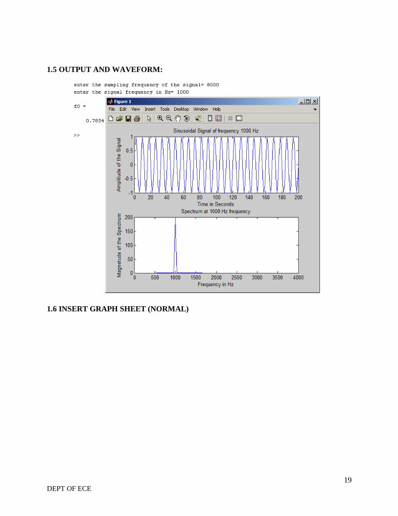
1.5 OUTPUT AND WAVEFORM:
1.6 INSERT GRAPH SHEET (NORMAL)
20 DEPT OF ECE
EXPERIMENT No 2
DFT AND IDFT OF A SEQUENCE
AIM: DFT and IDFT of a given sequence
TOOLS REQUIRED:
1. Mat lab software
2. Personal computer
THEORY:
In this program the Discrete Fourier Transform (DFT) of a sequence x[n] is generated by using
the formula,
N-1
X(k) = Σ x(n) e-2πjk / N
Where, X(k) DFT of sequence x[n]
n=0
N represents the sequence length and it is calculated by using the command „length‟. The DFT
of any sequence is the powerful computational tool for performing frequency analysis of
discrete-time signals.
PROGRAM: clc;
close all;
clear all;
xn=input('Enter the sequence x(n)'); %Get the sequence from user
ln=length(xn); %find the length of the sequence
xk=zeros(1,ln); %initilise an array of same size as that of input sequence
ixk=zeros(1,ln); %initilise an array of same size as that of input sequence
%code block to find the DFT of the sequence
%-----------------------------------------------------------
for k=0:ln-1
for n=0:ln-1
xk(k+1)=xk(k+1)+(xn(n+1)*exp((-i)*2*pi*k*n/ln));
end
end
%------------------------------------------------------------
21 DEPT OF ECE
%code block to plot the input sequence
%------------------------------------------------------------
t=0:ln-1;
subplot(311);
stem(t,xn);
ylabel ('Amplitude');
xlabel ('Time Index');
title('Input Sequence');
%---------------------------------------------------------------
magnitude=abs(xk); % Find the magnitudes of individual DFT points
%code block to plot the magnitude response
%------------------------------------------------------------
t=0:ln-1;
subplot(312);
stem(t,magnitude);
ylabel ('Amplitude');
xlabel ('K');
title('Magnitude Response');
%------------------------------------------------------------
% Code block to find the IDFT of the sequence
%------------------------------------------------------------
for n=0:ln-1
for k=0:ln-1
ixk(n+1)=ixk(n+1)+(xk(k+1)*exp(i*2*pi*k*n/ln));
end
end
ixk=ixk/ln;
%------------------------------------------------------------
%code block to plot the input sequence
t=0:ln-1;
subplot(313);
stem(t,ixk);ylabel ('Amplitude');xlabel ('Time Index');title('IDFT sequence');
22 DEPT OF ECE
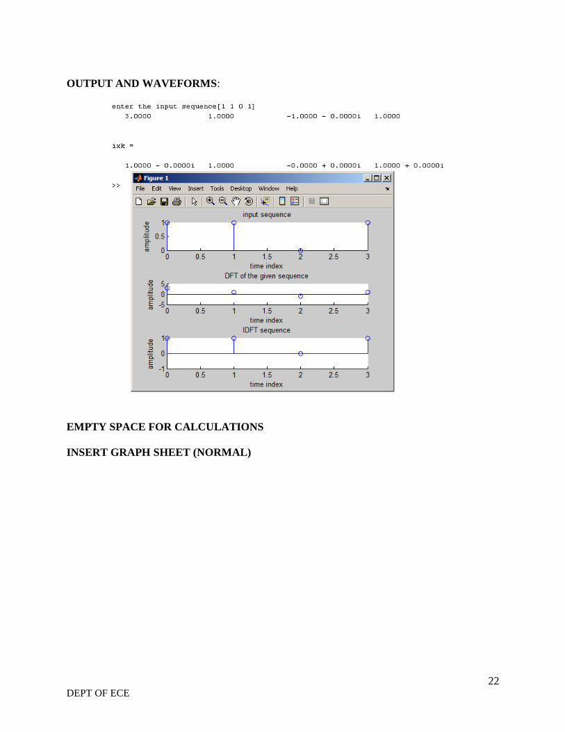
OUTPUT AND WAVEFORMS:
EMPTY SPACE FOR CALCULATIONS
INSERT GRAPH SHEET (NORMAL)
23 DEPT OF ECE
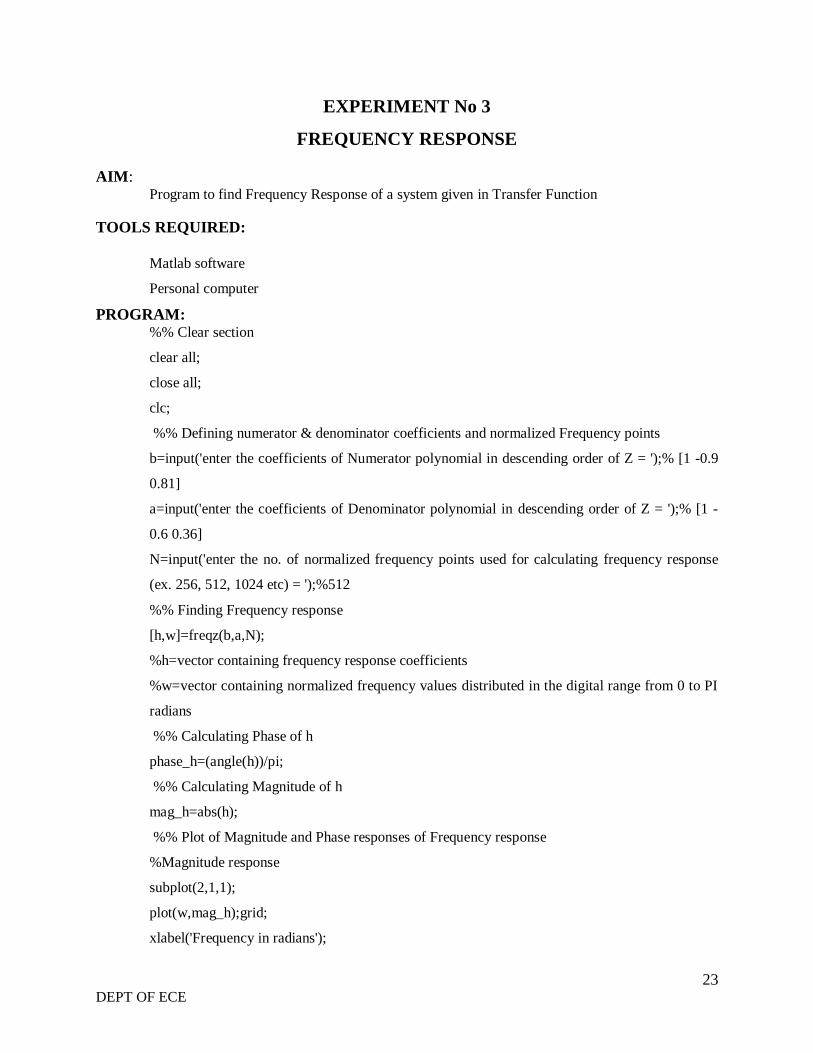
EXPERIMENT No 3
FREQUENCY RESPONSE
AIM: Program to find Frequency Response of a system given in Transfer Function
TOOLS REQUIRED:
Matlab software
Personal computer
PROGRAM: %% Clear section
clear all;
close all;
clc;
%% Defining numerator & denominator coefficients and normalized Frequency points
b=input('enter the coefficients of Numerator polynomial in descending order of Z = ');% [1 -0.9
0.81]
a=input('enter the coefficients of Denominator polynomial in descending order of Z = ');% [1 -
0.6 0.36]
N=input('enter the no. of normalized frequency points used for calculating frequency response
(ex. 256, 512, 1024 etc) = ');%512
%% Finding Frequency response
[h,w]=freqz(b,a,N);
%h=vector containing frequency response coefficients
%w=vector containing normalized frequency values distributed in the digital range from 0 to PI
radians
%% Calculating Phase of h
phase_h=(angle(h))/pi;
%% Calculating Magnitude of h
mag_h=abs(h);
%% Plot of Magnitude and Phase responses of Frequency response
%Magnitude response
subplot(2,1,1);
plot(w,mag_h);grid;
xlabel('Frequency in radians');
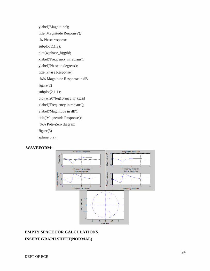
24 DEPT OF ECE
ylabel('Magnitude');
title('Magnitude Response');
% Phase response
subplot(2,1,2);
plot(w,phase_h);grid;
xlabel('Frequency in radians');
ylabel('Phase in degrees');
title('Phase Response');
%% Magnitude Response in dB
figure(2)
subplot(2,1,1);
plot(w,20*log10(mag_h));grid
xlabel('Frequency in radians');
ylabel('Magnitude in dB');
title('Magnetude Response');
%% Pole-Zero diagram
figure(3)
zplane(b,a);
WAVEFORM:
EMPTY SPACE FOR CALCULATIONS
INSERT GRAPH SHEET(NORMAL)
25 DEPT OF ECE
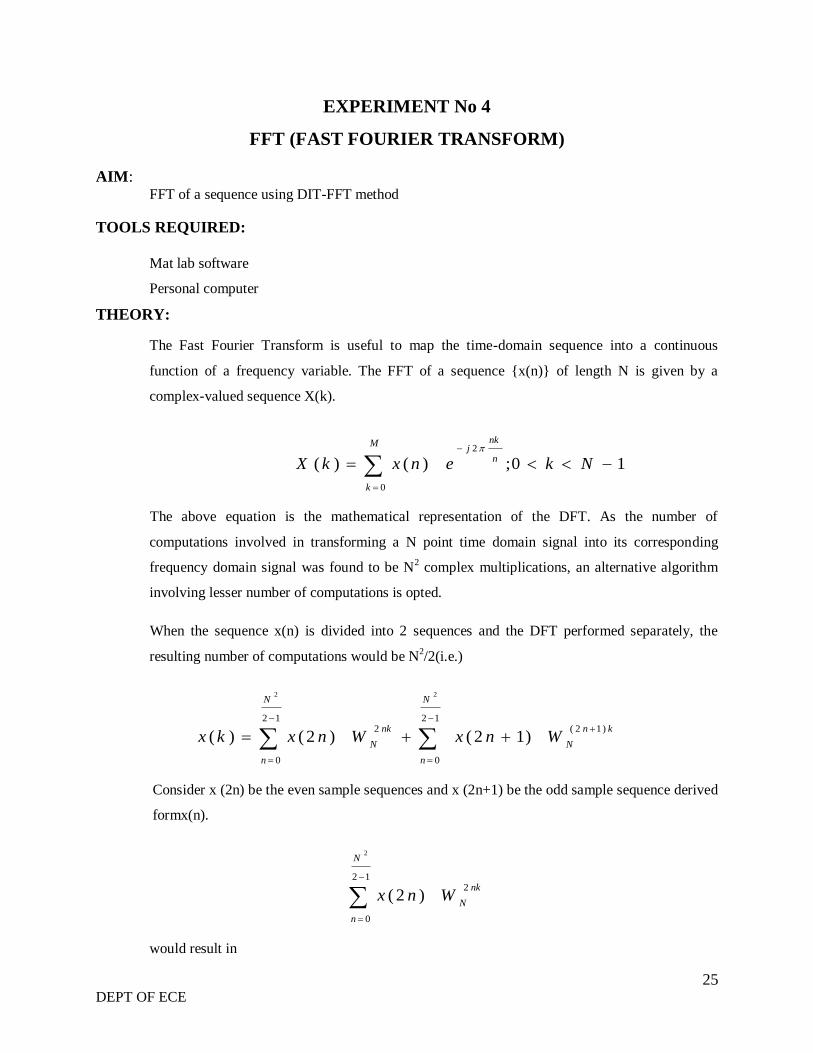
EXPERIMENT No 4
FFT (FAST FOURIER TRANSFORM)
AIM: FFT of a sequence using DIT-FFT method
TOOLS REQUIRED:
Mat lab software
Personal computer
THEORY:
The Fast Fourier Transform is useful to map the time-domain sequence into a continuous
function of a frequency variable. The FFT of a sequence {x(n)} of length N is given by a
complex-valued sequence X(k).
10;)()(
0
2
NkenxkX
M
k
n
nkj
The above equation is the mathematical representation of the DFT. As the number of
computations involved in transforming a N point time domain signal into its corresponding
frequency domain signal was found to be N2 complex multiplications, an alternative algorithm
involving lesser number of computations is opted.
When the sequence x(n) is divided into 2 sequences and the DFT performed separately, the
resulting number of computations would be N2/2(i.e.)
kn
N
N
n
N
n
nk
NWnxWnxkx
)12(12
0
12
0
2)12()2()(
2 2
Consider x (2n) be the even sample sequences and x (2n+1) be the odd sample sequence derived
formx(n).
12
0
2
2
)2(
N
n
nk
NWnx
would result in
26 DEPT OF ECE
(N/2)2multiplication‟s
12
0
)12(
2
)12(
N
n
kn
NWnx
Another (N/2)2
multiplication's finally resulting in (N/2)2 +
(N/2)2=
nsComputatioNNN
244
222
Further solving Eg.
k
N
nk
N
N
n
N
n
nk
NWWnxWnxkx
)2(12
0
12
0
2)12()2()(
2
)2(12
0
12
0
2)12()2(
nk
N
N
n
N
n
k
N
nk
NWnxWWnx
Dividing the sequence x(2n) into further 2 odd and even sequences would reduce the
computations.
WN is the twiddle factor
n
j
e
2
nkn
j
nk
NeW
2
22
NK
NN
NK
NWWW
2
22 n
n
j
kn
j
ee
27 DEPT OF ECE
kn
j
k
NeW
2
)sin(cos jW
k
N
)1(2
k
N
NK
NWW
k
N
NK
NWW
2
Employing this equation, we deduce
)2(12
0
12
0
2)12()2()(
2
nk
N
N
n
N
n
nk
NWnxWnxkx
)2(12
12
0
2)12()2()
2(
nk
N
N
N
n
K
N
nk
NWnxWWnx
Nkx
The time burden created by this large number of computations limits the usefulness of DFT in
many applications. Tremendous efforts devoted to develop more efficient ways of computing
DFT resulted in the above explained Fast Fourier Transform algorithm. This mathematical
shortcut reduces the number of calculations the DFT requires drastically. The above mentioned
radix-2 decimation in time FFT is employed for domain transformation.
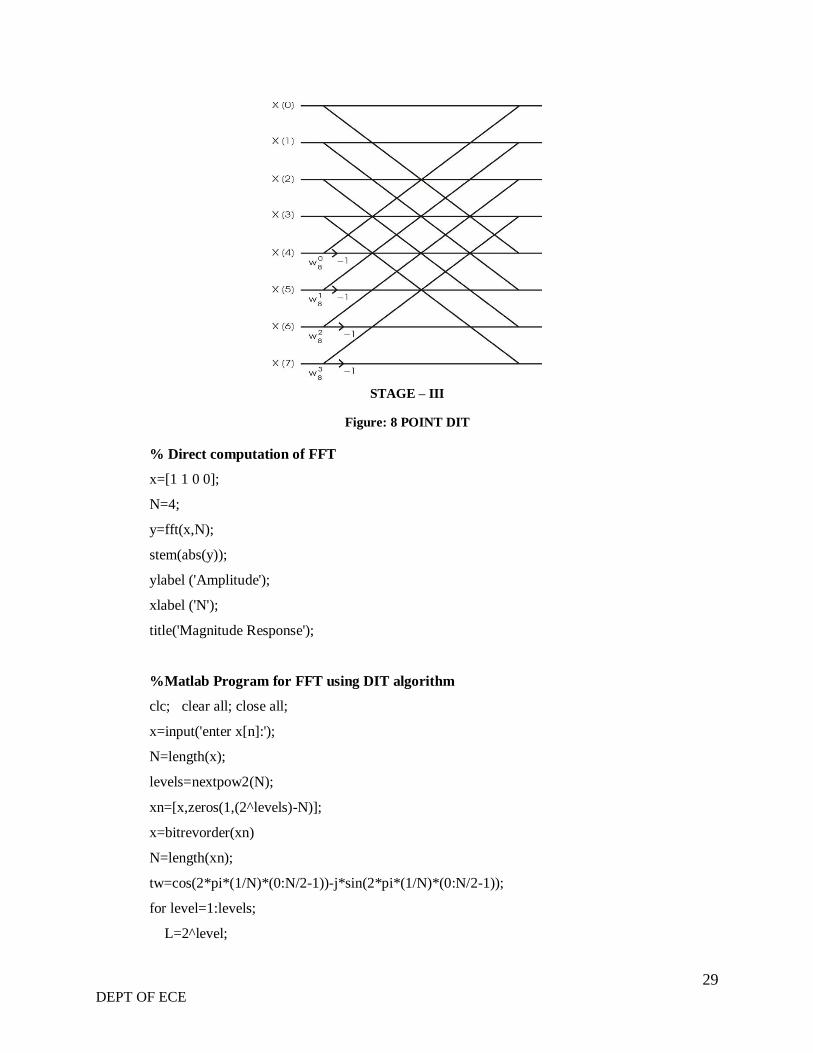
Dividing the DFT into smaller DFTs is the basis of the FFT. A radix-2 FFT divides the DFT into
two smaller DFTs, each of which is divided into smaller DFTs and so on, resulting in a
combination of two-point DFTs. The Decimation -In-Time (DIT) FFT divides the input (time)
sequence into two groups, one of even samples and the other of odd samples. N/2 point DFT are
performed on the these sub-sequences and their outputs are combined to form the N point DFT.
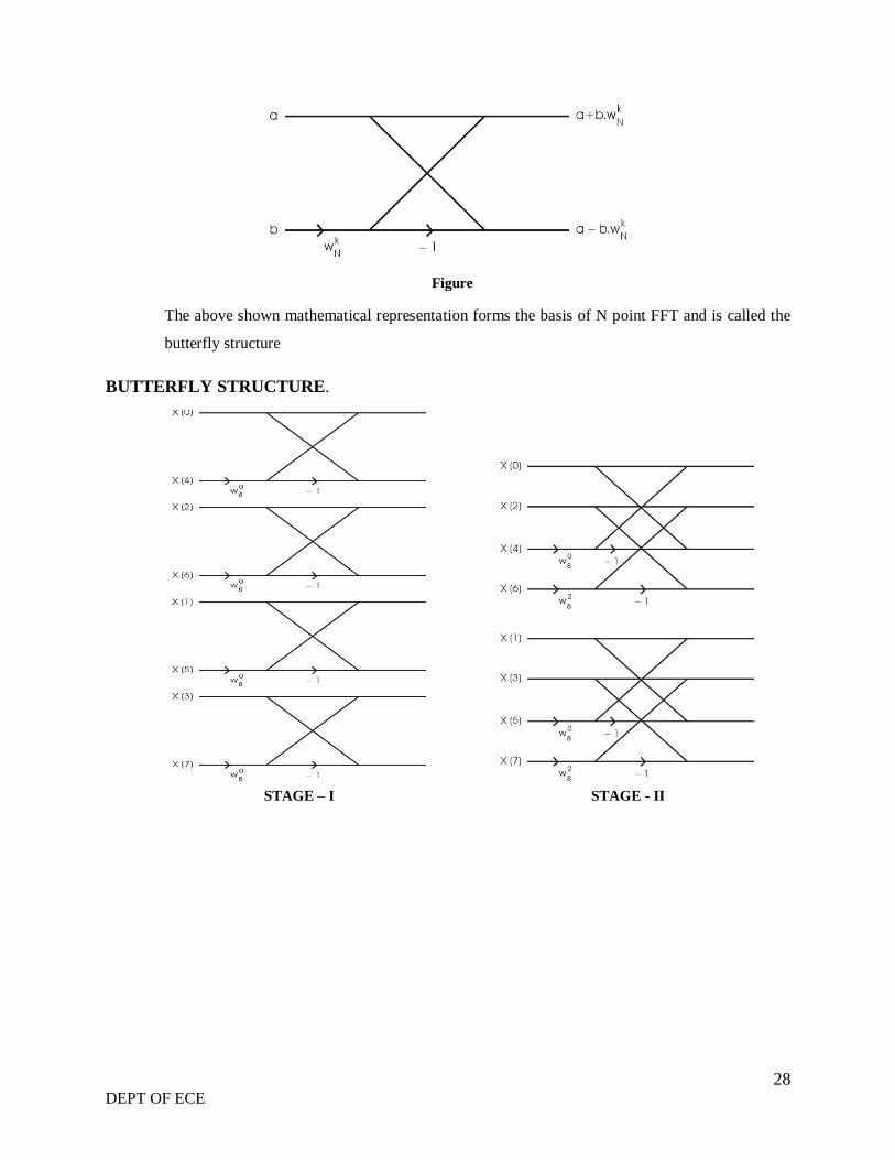
28 DEPT OF ECE
Figure
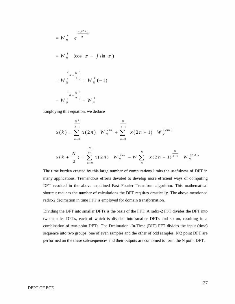
The above shown mathematical representation forms the basis of N point FFT and is called the
butterfly structure
BUTTERFLY STRUCTURE.
STAGE – I
STAGE - II
29 DEPT OF ECE
STAGE – III
Figure: 8 POINT DIT
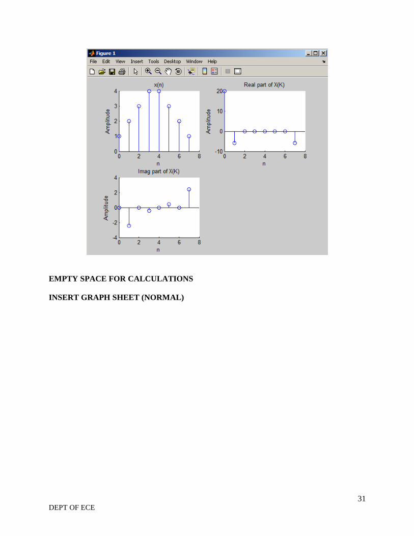
% Direct computation of FFT
x=[1 1 0 0];
N=4;
y=fft(x,N);
stem(abs(y));
ylabel ('Amplitude');
xlabel ('N');
title('Magnitude Response');
%Matlab Program for FFT using DIT algorithm
clc; clear all; close all;
x=input('enter x[n]:');
N=length(x);
levels=nextpow2(N);
xn=[x,zeros(1,(2^levels)-N)];
x=bitrevorder(xn)
N=length(xn);
tw=cos(2*pi*(1/N)*(0:N/2-1))-j*sin(2*pi*(1/N)*(0:N/2-1));
for level=1:levels;
L=2^level;
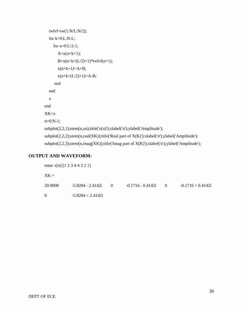
30 DEPT OF ECE
twlvl=tw(1:N/L:N/2);
for k=0:L:N-L;
for n=0:L/2-1;
A=x(n+k+1);
B=x(n+k+(L/2)+1)*twlvl(n+1);
x(n+k+1)=A+B;
x(n+k+(L/2)+1)=A-B;
end
end
x
end
XK=x
n=0:N-1;
subplot(2,2,1);stem(n,xn);title('x(n)');xlabel('n');ylabel('Amplitude');
subplot(2,2,2);stem(n,real(XK));title('Real part of X(K)');xlabel('n');ylabel('Amplitude');
subplot(2,2,3);stem(n,imag(XK));title('Imag part of X(K)');xlabel('n');ylabel('Amplitude');
OUTPUT AND WAVEFORM:
enter x[n]:[1 2 3 4 4 3 2 1]
XK =
20.0000 -5.8284 - 2.4142i 0 -0.1716 - 0.4142i 0 -0.1716 + 0.4142i
0 -5.8284 + 2.4142i
31 DEPT OF ECE
EMPTY SPACE FOR CALCULATIONS
INSERT GRAPH SHEET (NORMAL)

32 DEPT OF ECE
EXPERIMENT No 5
POWER SPECTRAL DENSITY
AIM:
Power spectral density
Tools Required:
Mat lab software
Personal computer
THEORY:
Power spectral density function (PSD) shows the strength of the variations (energy) as a function of
frequency. In other words, it shows at which frequencies variations are strong and at which frequencies
variations are weak. The unit of PSD is energy per frequency (width) and you can obtain energy within a
specific frequency range by integrating PSD within that frequency range. Computation of PSD is done
directly by the method called FFT or computing autocorrelation function and then transforming it.
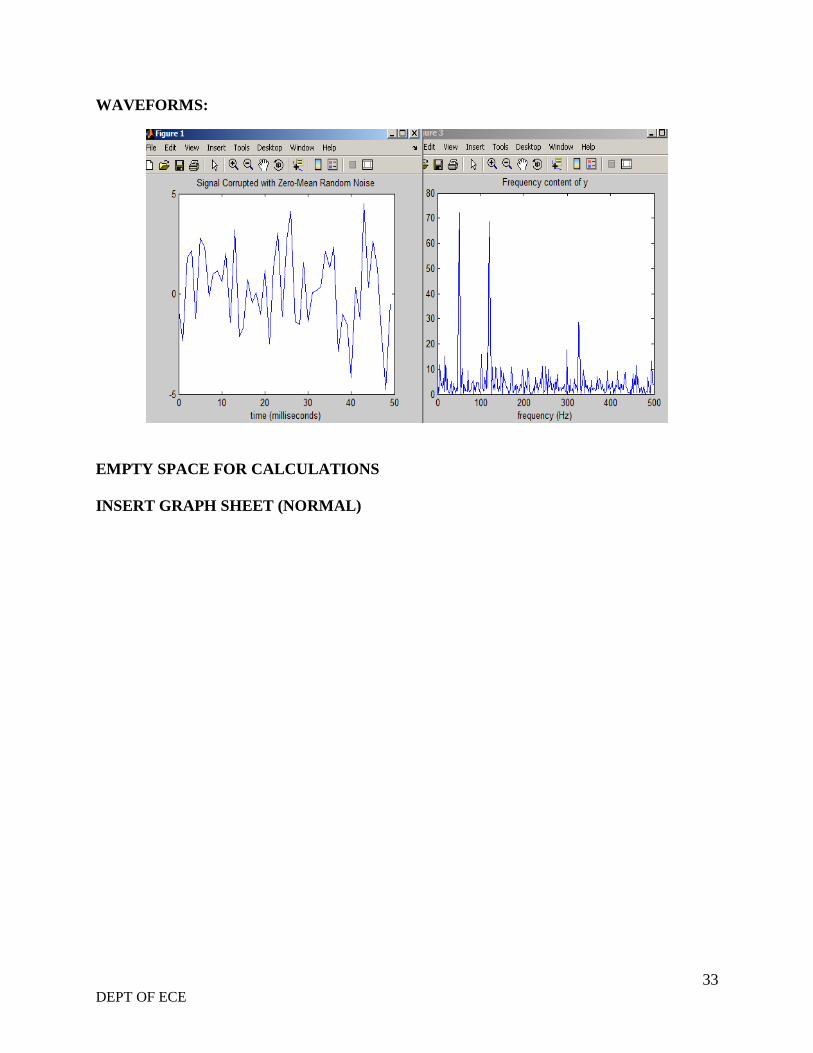
PROGRAM:
clc;clearall;close all;
t = 0:0.001:0.6;
x =sin(2*pi*50*t)+sin(2*pi*120*t);
y = x + 2*randn(size(t));
figure,plot(1000*t(1:50),y(1:50)) ;
title('Signal Corrupted with Zero-Mean Random Noise');
xlabel('time (milliseconds)');
Y = fft(y,512);
%The power spectral density, a measurement of the energy at various frequencies, is:
Pyy = Y.* conj(Y) / 512;
f = 1000*(0:256)/512;
figure,plot(f,Pyy(1:257));
title('Frequency content of y');
xlabel('frequency (Hz)');
33 DEPT OF ECE
WAVEFORMS:
EMPTY SPACE FOR CALCULATIONS
INSERT GRAPH SHEET (NORMAL)
34 DEPT OF ECE
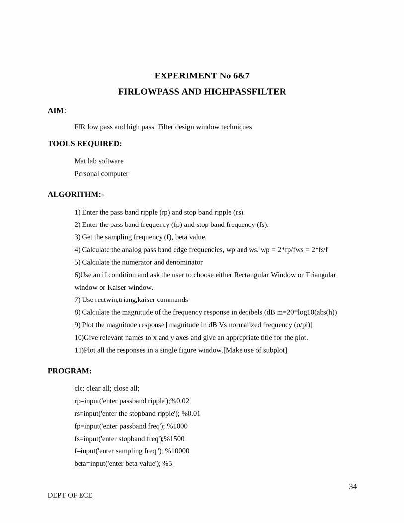
EXPERIMENT No 6&7
FIRLOWPASS AND HIGHPASSFILTER
AIM:
FIR low pass and high pass Filter design window techniques
TOOLS REQUIRED:
Mat lab software
Personal computer
ALGORITHM:-
1) Enter the pass band ripple (rp) and stop band ripple (rs).
2) Enter the pass band frequency (fp) and stop band frequency (fs).
3) Get the sampling frequency (f), beta value.
4) Calculate the analog pass band edge frequencies, wp and ws. wp = 2*fp/fws = 2*fs/f
5) Calculate the numerator and denominator
6)Use an if condition and ask the user to choose either Rectangular Window or Triangular
window or Kaiser window.
7) Use rectwin,triang,kaiser commands
8) Calculate the magnitude of the frequency response in decibels (dB m=20*log10(abs(h))
9) Plot the magnitude response [magnitude in dB Vs normalized frequency (o/pi)]
10)Give relevant names to x and y axes and give an appropriate title for the plot.
11)Plot all the responses in a single figure window.[Make use of subplot]
PROGRAM:
clc; clear all; close all;
rp=input('enter passband ripple');%0.02
rs=input('enter the stopband ripple'); %0.01
fp=input('enter passband freq'); %1000
fs=input('enter stopband freq');%1500
f=input('enter sampling freq '); %10000
beta=input('enter beta value'); %5
35 DEPT OF ECE
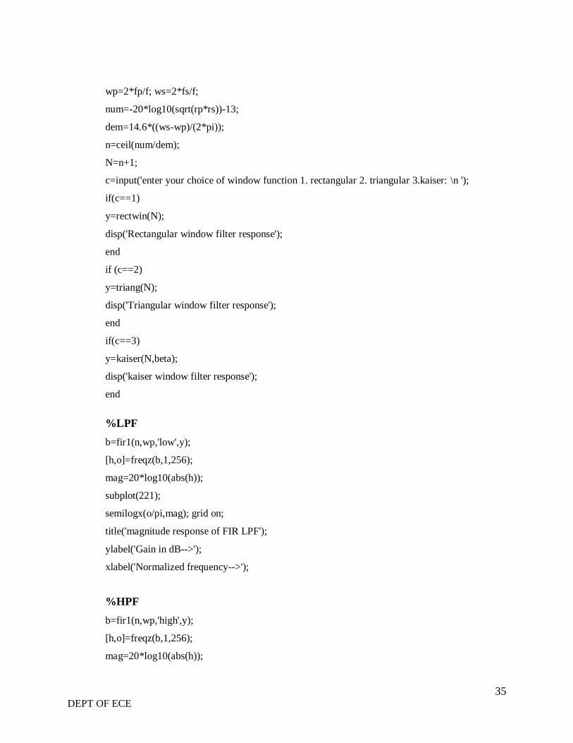
wp=2*fp/f; ws=2*fs/f;
num=-20*log10(sqrt(rp*rs))-13;
dem=14.6*((ws-wp)/(2*pi));
n=ceil(num/dem);
N=n+1;
c=input('enter your choice of window function 1. rectangular 2. triangular 3.kaiser: \n ');
if(c==1)
y=rectwin(N);
disp('Rectangular window filter response');
end
if (c==2)
y=triang(N);
disp('Triangular window filter response');
end
if(c==3)
y=kaiser(N,beta);
disp('kaiser window filter response');
end
%LPF
b=fir1(n,wp,'low',y);
[h,o]=freqz(b,1,256);
mag=20*log10(abs(h));
subplot(221);
semilogx(o/pi,mag); grid on;
title('magnitude response of FIR LPF');
ylabel('Gain in dB-->');
xlabel('Normalized frequency-->');
%HPF
b=fir1(n,wp,'high',y);
[h,o]=freqz(b,1,256);
mag=20*log10(abs(h));
36 DEPT OF ECE
subplot(222);
semilogx(o/pi,mag); grid on;
title('magnitude response of FIR HPF');
ylabel('Gain in dB-->');
xlabel('Normalized frequency-->');
%BPF
wn=[wpws];
b=fir1(n,wn,y);
[h,o]=freqz(b,1,256);
mag=20*log10(abs(h));
subplot(223);
semilogx(o/pi,mag); grid on;
title('magnitude response of FIR BPF');
ylabel('Gain in dB-->');
xlabel('Normalized frequency-->');
%BSF
b=fir1(n,wn,'stop',y);
[h,o]=freqz(b,1,256);
mag=20*log10(abs(h));
subplot(224);
semilogx(o/pi,mag); grid on;
title('magnitude response of FIR BSF');
ylabel('Gain in dB-->');
xlabel('Normalized frequency-->');
37 DEPT OF ECE
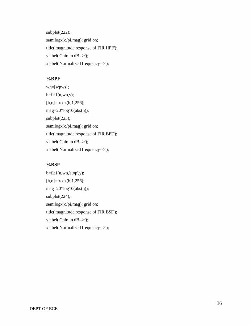
OUTPUT AND WAVEFORM:
EMPTY SPACE FOR CALCULATIONS
INSERT GRAPH SHEET (SEMILOG)
38 DEPT OF ECE
EXPERIMENT No 8&9
IIR LOWPASS AND HIGHPASSFILTER
AIM:
IIR lowpass and highpass Filter design
TOOLS REQUIRED:
Mat lab software
Personal computer
THEORY:
The IIR filter can realize both the poles and zeroes of a system because it has a rational transfer
function, described by polynomials in z in both the numerator and the denominator:
N
k
k
k
M
k
k
k
Za
zb
zH
1
0)(
The difference equation for such a system is described by the following:
N
k
k
M
k
kknyaknxbny
10
)()()(
M and N are order of the two polynomialsbkand ak are the filter coefficients. These filter
coefficients are generated using FDS (Filter Design software or Digital Filter design package).
IIR filters can be expanded as infinite impulse response filters. In designing IIR filters, cutoff
frequencies of the filters should be mentioned. The order of the filter can be estimated using
butter worth polynomial. That‟s why the filters are named as butter worth filters. Filter
coefficients can be found and the response can be plotted.
ALGORITHM:-
1) Enter the pass band ripple (alphap) and stop band ripple (alphas).
2) Enter the pass band frequency (fp) and stop band frequency (fs).
3) Get the sampling frequency (F).
39 DEPT OF ECE
4) Calculate the analog pass band edge frequencies, omegap and omegas. omegap =
2*fp/Fomegas = 2*fs/F
5) Calculate the order and 3dB cutoff frequency of the analog filter. [Make use of the
following function] [n,wn]=buttord(omegap,omegas,rp,rs)
6) Design an nth order analog lowpass Butter worth filter using the following statement.
[b,a]=butter(n,wn, „low‟)
7) Find the complex frequency response of the filter by using freqz( ) function
[h,om]=freqz(b,a,w) where, w = 0:0.01:pi This function returns complex frequency
response vector „h‟ and frequency vector „om‟ in radians/samples of the filter.
8) Calculate the magnitude of the frequency response in decibels (dB
m=20*log10(abs(h))
9) Plot the magnitude response [magnitude in dB Vs normalized frequency (om/pi)]
10) Calculate the phase response using an = angle(h)
11) Plot the phase response [phase in radians Vs normalized frequency (om/pi)]
12) Give relevant names to x and y axes and give an appropriate title for the plot.
13) Plot all the responses in a single figure window.[Make use of subplot]
PROGRAM:
clc;clearall;close all;
disp('IIR filter design specifications:');
alpha
p=input('enter the passband attenuation:'); %0.15
alphas=input('enter the stopband attenuation:'); %60
fp=input('enter the passband frequency:'); % 1500
fs=input('enter the stopband frequency:'); % 3000
F=input('enter the sampling frequency:'); % 7000
omegap=2*fp/F;
omegas=2*fs/F;
%To find the cutoff frequency and order of the filter
[n,wn]=buttord(omegap,omegas,alphap,alphas);
%To find the system function of the lowpass filter
[b,a]=butter(n,wn,'low');%'high'
w=0:0.01:pi;
[h,om]=freqz(b,a,w);
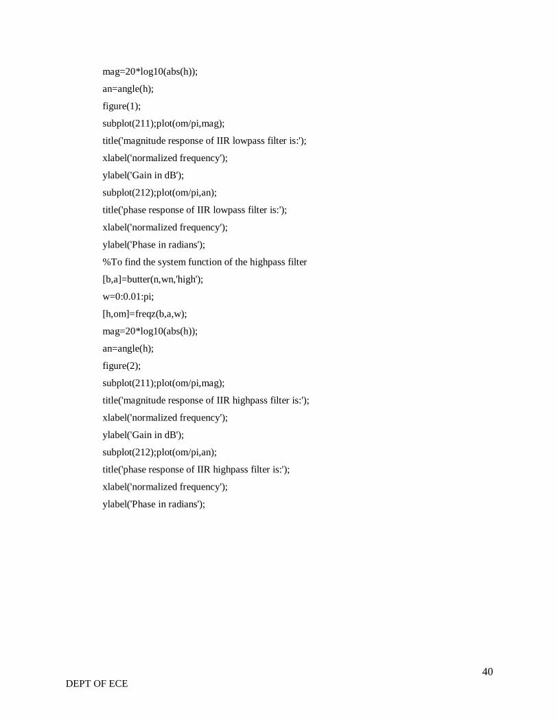
40 DEPT OF ECE
mag=20*log10(abs(h));
an=angle(h);
figure(1);
subplot(211);plot(om/pi,mag);
title('magnitude response of IIR lowpass filter is:');
xlabel('normalized frequency');
ylabel('Gain in dB');
subplot(212);plot(om/pi,an);
title('phase response of IIR lowpass filter is:');
xlabel('normalized frequency');
ylabel('Phase in radians');
%To find the system function of the highpass filter
[b,a]=butter(n,wn,'high');
w=0:0.01:pi;
[h,om]=freqz(b,a,w);
mag=20*log10(abs(h));
an=angle(h);
figure(2);
subplot(211);plot(om/pi,mag);
title('magnitude response of IIR highpass filter is:');
xlabel('normalized frequency');
ylabel('Gain in dB');
subplot(212);plot(om/pi,an);
title('phase response of IIR highpass filter is:');
xlabel('normalized frequency');
ylabel('Phase in radians');
41 DEPT OF ECE
OUTPUT:
EMPTY SPACE FOR CALCULATIONS
INSERT GRAPH SHEET (SEMILOG)
42 DEPT OF ECE
EXPERIMENT No 10
SINUSOIDAL SIGNAL THROUGH FILTERING
AIM:
Program for generation of Sinusoidal Signal through filtering
TOOLS REQUIRED:
Mat lab software
Personal computer
PROGRAM:
%% Clear Section
clear all;closeall;clc;
%% Signal Frequency and Sampling frequency
f_hz=1000; % Signal frequency (Change this value and test)
fs=8000; % Sampling frequency (change this value and test)
f0=2*pi*f_hz/fs; % Sampled Signal Frequency in Radians
t=0:1/fs:1; % Time Vector for 1 Second duration
x=[1 zeros(1,length(t)) ] % Initializing the input sequence to zero
%% Calculation of numerator coefficients
b0=0;
b1=sin(f0);
%% Calculation of denominator coefficients
a0=1;
a1=-2*sin(f0);
a2=1;
b=[b0 b1]; % Numerator coefficients
a=[a0 a1 a2]; % Denominator coefficients
%% Filtering Operation
y=filter(b,a,x);
%% Plot of Signal and its Spectrum
subplot(2,1,1)
plot(t(1:200),y(1:200)); % Select only 200 points for clear plot
xlabel('Time in Seconds');
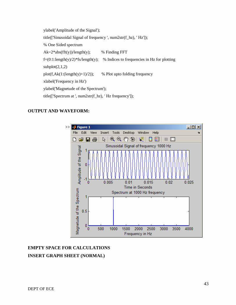
43 DEPT OF ECE
ylabel('Amplitude of the Signal');
title(['Sinusoidal Signal of frequency ', num2str(f_hz), ' Hz']);
% One Sided spectrum
Ak=2*abs(fft(y))/length(y); % Finding FFT
f=(0:1:length(y)/2)*fs/length(y); % Indices to frequencies in Hz for plotting
subplot(2,1,2)
plot(f,Ak(1:(length(y)+1)/2)); % Plot upto folding frequency
xlabel('Frequency in Hz')
ylabel('Magnetude of the Spectrum');
title(['Spectrum at ', num2str(f_hz), ' Hz frequency']);
OUTPUT AND WAVEFORM:
EMPTY SPACE FOR CALCULATIONS
INSERT GRAPH SHEET (NORMAL)
44 DEPT OF ECE
EXPERIMENT No 11
DECIMATION BY FACTOR D
AIM:
Decimation by factor D
TOOLS REQUIRED:
Mat lab software
Personal computer
THEORY:
Sampling rate conversion (SRC) is a process of converting a discrete-time signal at a given rate
to a different rate. This technique is encountered in many application areas such as:
Digital Audio
Communications systems
Speech Processing
Antenna Systems
Radar Systems etc
Sampling rates may be changed upward or downward. Increasing the sampling rate is called
interpolation, and decreasing the sampling rate is called decimation. Reducing the sampling rate
by a factor of M is achieved by discarding every M-1 samples, or, equivalently keeping every
Mthsample. Increasing the sampling rate by a factor of L (interpolation by factor L) is achieved
by inserting L-1 zeros into the output stream after every sample from the input stream of
samples.
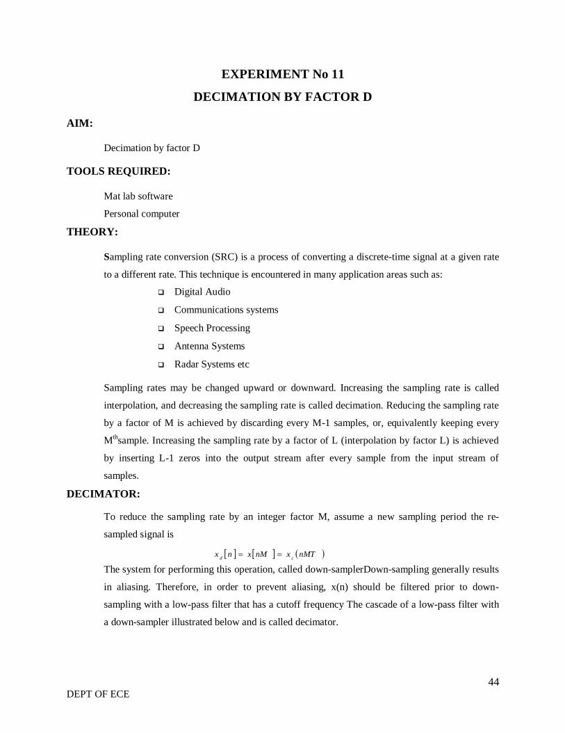
DECIMATOR:
To reduce the sampling rate by an integer factor M, assume a new sampling period the re-
sampled signal is
The system for performing this operation, called down-samplerDown-sampling generally results
in aliasing. Therefore, in order to prevent aliasing, x(n) should be filtered prior to down-
sampling with a low-pass filter that has a cutoff frequency The cascade of a low-pass filter with
a down-sampler illustrated below and is called decimator.
nMTxnMxnxcd
45 DEPT OF ECE
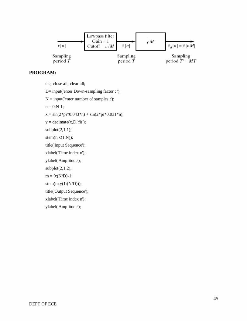
PROGRAM:
clc; close all; clear all;
D= input('enter Down-sampling factor : ');
N = input('enter number of samples :');
n = 0:N-1;
x = sin(2*pi*0.043*n) + sin(2*pi*0.031*n);
y = decimate(x,D,'fir');
subplot(2,1,1);
stem(n,x(1:N));
title('Input Sequence');
xlabel('Time index n');
ylabel('Amplitude');
subplot(2,1,2);
m = 0:(N/D)-1;
stem(m,y(1:(N/D)));
title('Output Sequence');
xlabel('Time index n');
ylabel('Amplitude');
46 DEPT OF ECE
OUTPUT AND WAVEFORM:
EMPTY SPACE FOR CALCULATIONS
INSERT GRAPH SHEET (NORMAL)
47 DEPT OF ECE
EXPERIMENT No 12
INTERPOLATION BY A FACTOR I
AIM:
Interpolation by a factor I
TOOLS REQUIRED:
Mat lab software
Personal computer
THEORY:
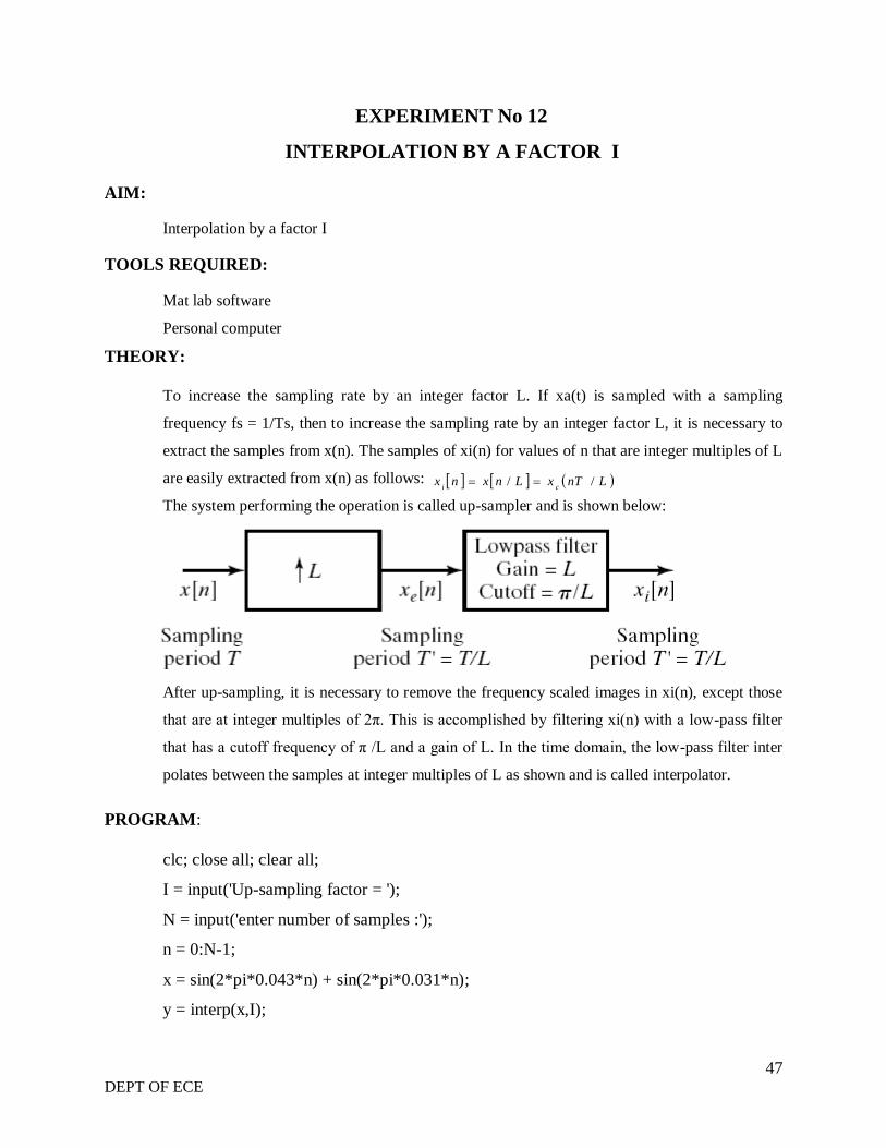
To increase the sampling rate by an integer factor L. If xa(t) is sampled with a sampling
frequency fs = 1/Ts, then to increase the sampling rate by an integer factor L, it is necessary to
extract the samples from x(n). The samples of xi(n) for values of n that are integer multiples of L
are easily extracted from x(n) as follows:
The system performing the operation is called up-sampler and is shown below:
After up-sampling, it is necessary to remove the frequency scaled images in xi(n), except those
that are at integer multiples of 2π. This is accomplished by filtering xi(n) with a low-pass filter
that has a cutoff frequency of π /L and a gain of L. In the time domain, the low-pass filter inter
polates between the samples at integer multiples of L as shown and is called interpolator.
PROGRAM:
clc; close all; clear all;
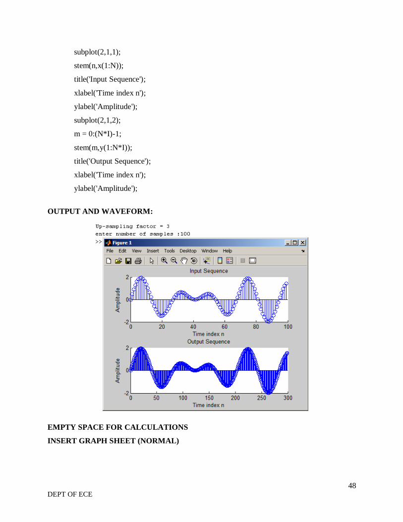
I = input('Up-sampling factor = ');
N = input('enter number of samples :');
n = 0:N-1;
x = sin(2*pi*0.043*n) + sin(2*pi*0.031*n);
y = interp(x,I);
LnTxLnxnxci
//
48 DEPT OF ECE
subplot(2,1,1);
stem(n,x(1:N));
title('Input Sequence');
xlabel('Time index n');
ylabel('Amplitude');
subplot(2,1,2);
m = 0:(N*I)-1;
stem(m,y(1:N*I));
title('Output Sequence');
xlabel('Time index n');
ylabel('Amplitude');
OUTPUT AND WAVEFORM:
EMPTY SPACE FOR CALCULATIONS
INSERT GRAPH SHEET (NORMAL)
49 DEPT OF ECE
EXPERIMENT No 13
SAMPLING RATE CONVERSION BY A FACTOR I/D
AIM:
Sampling rate conversion by a factor I/D
TOOLS REQUIRED:
Mat lab software
Personal computer
THEORY:
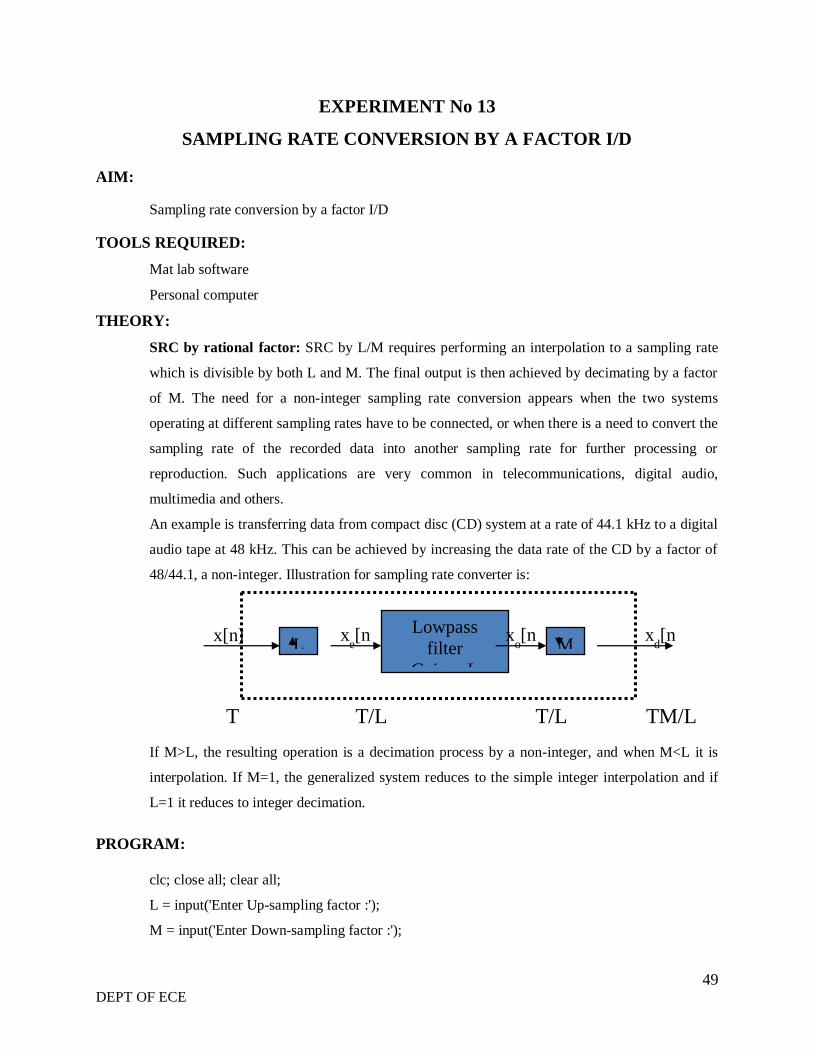
SRC by rational factor: SRC by L/M requires performing an interpolation to a sampling rate
which is divisible by both L and M. The final output is then achieved by decimating by a factor
of M. The need for a non-integer sampling rate conversion appears when the two systems
operating at different sampling rates have to be connected, or when there is a need to convert the
sampling rate of the recorded data into another sampling rate for further processing or
reproduction. Such applications are very common in telecommunications, digital audio,
multimedia and others.
An example is transferring data from compact disc (CD) system at a rate of 44.1 kHz to a digital
audio tape at 48 kHz. This can be achieved by increasing the data rate of the CD by a factor of
48/44.1, a non-integer. Illustration for sampling rate converter is:
If M>L, the resulting operation is a decimation process by a non-integer, and when M<L it is
interpolation. If M=1, the generalized system reduces to the simple integer interpolation and if
L=1 it reduces to integer decimation.
PROGRAM:
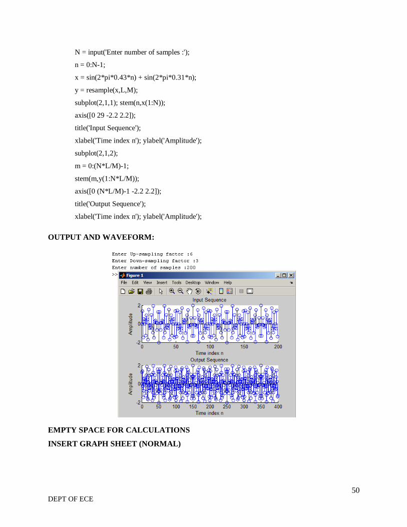
clc; close all; clear all;
L = input('Enter Up-sampling factor :');
M = input('Enter Down-sampling factor :');
Lowpass
filter
Gain = L
Cutoff =
min(p/L,
p/M)
L M x
d[nx[n] x
e[n x
o[n
T T/L T/L TM/L
50 DEPT OF ECE
N = input('Enter number of samples :');
n = 0:N-1;
x = sin(2*pi*0.43*n) + sin(2*pi*0.31*n);
y = resample(x,L,M);
subplot(2,1,1); stem(n,x(1:N));
axis([0 29 -2.2 2.2]);
title('Input Sequence');
xlabel('Time index n'); ylabel('Amplitude');
subplot(2,1,2);
m = 0:(N*L/M)-1;
stem(m,y(1:N*L/M));
axis([0 (N*L/M)-1 -2.2 2.2]);
title('Output Sequence');
xlabel('Time index n'); ylabel('Amplitude');
OUTPUT AND WAVEFORM:
EMPTY SPACE FOR CALCULATIONS
INSERT GRAPH SHEET (NORMAL)

51 DEPT OF ECE
EXPERIMENT No 14
IMPULSE RESPONSE
AIM:
Impulse Response of First order and Second order systems
TOOLS REQUIRED:
Mat lab software
Personal computer
PROGRAM:
clear all;close all; clc;
%y(n)+y(n-1)+0.9y(n-2)=x(n)+0.5x(n-1)+0.5x(n-2)
%a=input('enter the coefficients of denominator polynomial= ');
%b=input('enter the coefcients of numerator polynomial= ');
b=[1 1 0.9];
a=[1 0.5 0.5];
N=32; % length of input sequence
x=[1 zeros(1,N)]
y=filter(b,a,x)
subplot(2,1,1)
stem(1:length(x),x);
xlabel('Time');
ylabel('Amplitude');
title('Impulse Sequence');
subplot(2,1,2)
stem(1:length(y),y);
xlabel('Time');
ylabel('Amplitude');
title('Impulse Response Sequence');

52 DEPT OF ECE
OUTPUT AND WAVEFORM:
EMPTY SPACE FOR CALCULATIONS
INSERT GRAPH SHEET (NORMAL)
53 DEPT OF ECE
EXPERIEMENTS
(Using DSP Kit)
INTRODUCTION TO DSP PROCESSORS
A signal can be defined as a function that conveys information, generally about the state or
behavior of a physical system. There are two basic types of signals viz Analog (continuous time
signals which are defined along a continuum of times) and Digital (discrete-time).
Remarkably, under reasonable constraints, a continuous time signal can be adequately
represented by samples, obtaining discrete time signals. Thus digital signal processing is an ideal
choice for anyone who needs the performance advantage of digital manipulation along with
today‟s analog reality.
Hence a processor which is designed to perform the special operations(digital manipulations) on
the digital signal within very less time can be called as a Digital signal processor. The difference
between a DSP processor, conventional microprocessor and a microcontroller are listed below.
Microprocessor: or General Purpose Processor such as Intel xx86 or Motorola 680xx
Family
Contains - only CPU
-No RAM
-No ROM
-No I/O ports
-No Timer
MICROCONTROLLER
Such as 8051 familyContains - CPU
- RAM
- ROM
-I/O ports
- Timer &
- Interrupt circuitry
Some Micro Controllers also contain A/D, D/A and Flash Memory
DSP PROCESSORS
Such as Texas instruments and Analog DevicesContains
- CPU
54 DEPT OF ECE
- RAM
- ROM
- I/O ports
- Timer
Optimized for
- fast arithmetic
- Extended precision
- Dual operand fetch
- Zero overhead loop
- Circular buffering
The basic features of a DSP Processor are
Feature Use
Fast-Multiply accumulate Most DSP algorithms, including filtering,
transforms, etc. are multiplication- intensive
Multiple – access memory architecture Many data-intensive DSP operations require
reading a program instruction and multiple data
items during each instruction cycle for best
performance
Specialized addressing modes Efficient handling of data arrays and first-in,
first-out buffers in memory
Specialized program control Efficient control of loops for many iterative
DSP algorithms. Fast interrupt handling for
frequent I/O operations.
On-chip peripherals and I/O interfaces On-chip peripherals like A/D converters allow
for small low cost system designs. Similarly
I/O interfaces tailored for common peripherals
allow clean interfaces to off-chip I/O devices.
A digital signal processor (DSP) is an integrated circuit designed for high-speed data
manipulations, and is used in audio, communications, image manipulation, and other data-
acquisition and data-control applications. The microprocessors used in personal computers are
optimized for tasks involving data movement and inequality testing. The typical applications
requiring such capabilities are word processing, database management, spread sheets, etc. When
55 DEPT OF ECE
it comes to mathematical computations the traditional microprocessor are deficient particularly
where real-time performance is required. Digital signal processors are microprocessors
optimized for basic mathematical calculations such as additions and multiplications.
FIXED VERSUS FLOATING POINT:
Digital Signal Processing can be divided into two categories, fixed point and floating point
which refer to the format used to store and manipulate numbers within the devices. Fixed point
DSPs usually represent each number with a minimum of 16 bits, although a different length can
be used. There are four common ways that these 216 i,e., 65,536 possible bit patterns can
represent a number. In unsigned integer, the stored number can take on any integer value from 0
to 65,535, signed integer uses two's complement to include negative numbers from -32,768 to
32,767. With unsigned fraction notation, the 65,536 levels are spread uniformly between 0 and 1
and the signed fraction format allows negative numbers, equally spaced between -1 and 1. The
floating point DSPs typically use a minimum of 32 bits to store each value. This results in many
more bit patterns than for fixed point, 232 i,e., 4,294,967,296 to be exact. All floating point
DSPs can also handle fixed point numbers, a necessity to implement counters, loops, and signals
coming from the ADC and going to the DAC. However, this doesn't mean that fixed point math
will be carried out as quickly as the floating point operations; it depends on the internal
architecture.
C VERSUS ASSEMBLY:
DSPs are programmed in the same languages as other scientific and engineering applications,
usually assembly or C. Programs written in assembly can execute faster, while programs written
in C are easier to develop and maintain. In traditional applications, such as programs run on PCs
and mainframes, C is almost always the first choice. If assembly is used at all, it is restricted to
short subroutines that must run with the utmost speed.
HOW FAST ARE DSPS?
The primary reason for using a DSP instead of a traditional microprocessor is speed: the ability
to move samples into the device and carry out the needed mathematical operations, and output
the processed data. The usual way of specifying the fastness of a DSP is: fixed point systems are
often quoted in MIPS (million integer operations per second). Likewise, floating point devices
can be specified in MFLOPS (million floating point operations per second).
56 DEPT OF ECE
TMS320 FAMILY:
The Texas Instruments TMS320 family of DSP devices covers a wide range, from a 16-bit fixed-
point device to a single-chip parallel-processor device. In the past, DSPs were used only in
specialized applications. Now they are in many mass-market consumer products that are
continuously entering new market segments. The Texas Instruments TMS320 family of DSP
devices and their typical applications are mentioned below.
C1x, C2x, C2xx, C5x, and C54x:
The width of the data bus on these devices is 16 bits. All have modified Harvard architectures.
They have been used in toys, hard disk drives, modems, cellular phones, and active car
suspensions.
C3x:
The width of the data bus in the C3x series is 32 bits. Because of the reasonable cost and
floating-point performance, these are suitable for many applications. These include almost any
filters, analyzers, hi-fi systems, voice-mail, imaging, bar-code readers, motor control, 3D
graphics, or scientific processing.
C4x:
This range is designed for parallel processing. The C4x devices have a 32-bit data bus and are
floating-point. They have an optimized on-chip communication channel, which enables a
number of them to be put together to form a parallel-processing cluster. The C4x range devices
have been used in virtual reality, image recognition, telecom routing, and parallel-processing
systems.
C6x:
The C6x devices feature Velocity, an advanced very long instruction word (VLIW) architecture
developed by Texas Instruments. Eight functional units, including two multipliersand six
arithmetic logic units (ALUs), provide 1600 MIPS of cost-effective performance. The C6x DSPs
are optimized for multi-channel, multifunction applications, including wireless base stations,
pooled modems, remote-access servers, digital subscriber loop systems, cable modems, and
multi-channel telephone systems.
57 DEPT OF ECE
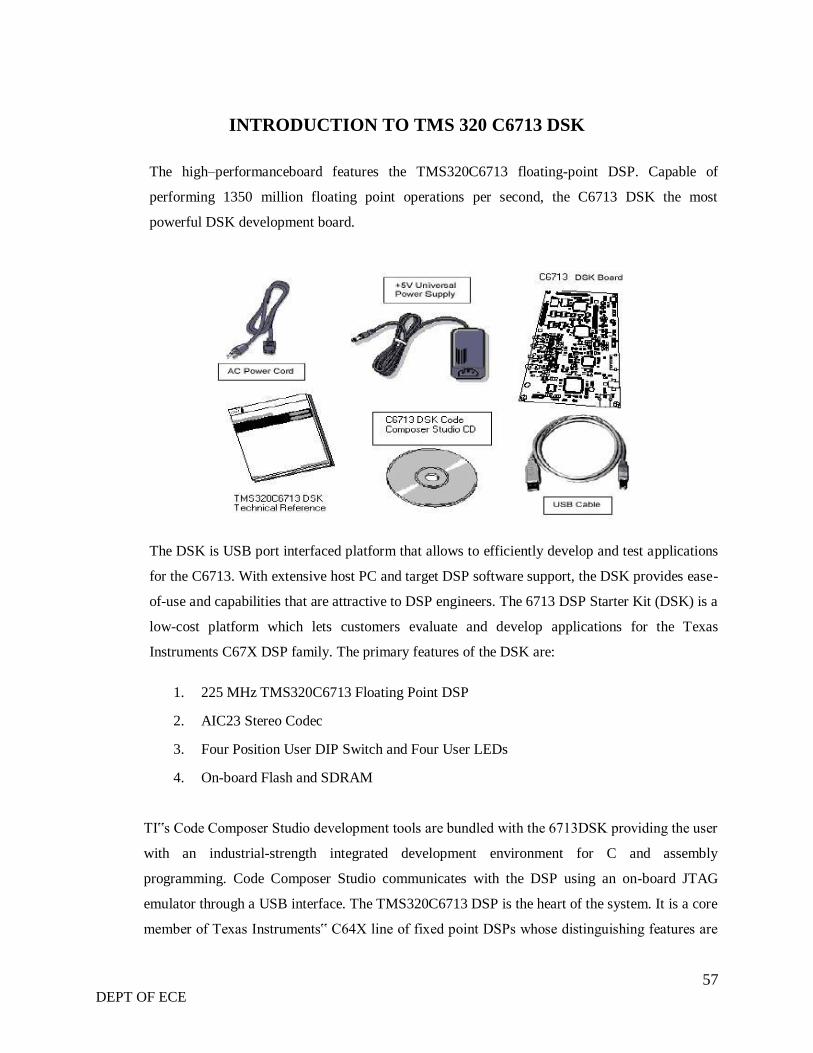
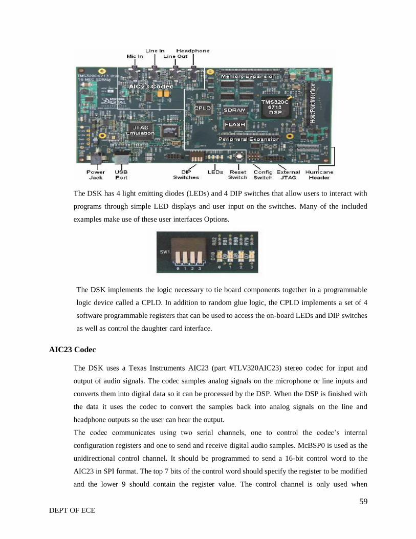
INTRODUCTION TO TMS 320 C6713 DSK
The high–performanceboard features the TMS320C6713 floating-point DSP. Capable of
performing 1350 million floating point operations per second, the C6713 DSK the most
powerful DSK development board.
The DSK is USB port interfaced platform that allows to efficiently develop and test applications
for the C6713. With extensive host PC and target DSP software support, the DSK provides ease-
of-use and capabilities that are attractive to DSP engineers. The 6713 DSP Starter Kit (DSK) is a
low-cost platform which lets customers evaluate and develop applications for the Texas
Instruments C67X DSP family. The primary features of the DSK are:
1. 225 MHz TMS320C6713 Floating Point DSP
2. AIC23 Stereo Codec
3. Four Position User DIP Switch and Four User LEDs
4. On-board Flash and SDRAM
TI‟s Code Composer Studio development tools are bundled with the 6713DSK providing the user
with an industrial-strength integrated development environment for C and assembly
programming. Code Composer Studio communicates with the DSP using an on-board JTAG
emulator through a USB interface. The TMS320C6713 DSP is the heart of the system. It is a core
member of Texas Instruments‟ C64X line of fixed point DSPs whose distinguishing features are
58 DEPT OF ECE
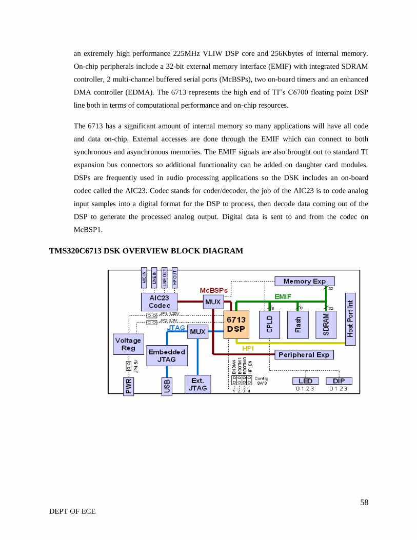
an extremely high performance 225MHz VLIW DSP core and 256Kbytes of internal memory.
On-chip peripherals include a 32-bit external memory interface (EMIF) with integrated SDRAM
controller, 2 multi-channel buffered serial ports (McBSPs), two on-board timers and an enhanced
DMA controller (EDMA). The 6713 represents the high end of TI‟s C6700 floating point DSP
line both in terms of computational performance and on-chip resources.
The 6713 has a significant amount of internal memory so many applications will have all code
and data on-chip. External accesses are done through the EMIF which can connect to both
synchronous and asynchronous memories. The EMIF signals are also brought out to standard TI
expansion bus connectors so additional functionality can be added on daughter card modules.
DSPs are frequently used in audio processing applications so the DSK includes an on-board
codec called the AIC23. Codec stands for coder/decoder, the job of the AIC23 is to code analog
input samples into a digital format for the DSP to process, then decode data coming out of the
DSP to generate the processed analog output. Digital data is sent to and from the codec on
McBSP1.
TMS320C6713 DSK OVERVIEW BLOCK DIAGRAM
59 DEPT OF ECE
The DSK has 4 light emitting diodes (LEDs) and 4 DIP switches that allow users to interact with
programs through simple LED displays and user input on the switches. Many of the included
examples make use of these user interfaces Options.
The DSK implements the logic necessary to tie board components together in a programmable
logic device called a CPLD. In addition to random glue logic, the CPLD implements a set of 4
software programmable registers that can be used to access the on-board LEDs and DIP switches
as well as control the daughter card interface.
AIC23 Codec
The DSK uses a Texas Instruments AIC23 (part #TLV320AIC23) stereo codec for input and
output of audio signals. The codec samples analog signals on the microphone or line inputs and
converts them into digital data so it can be processed by the DSP. When the DSP is finished with
the data it uses the codec to convert the samples back into analog signals on the line and
headphone outputs so the user can hear the output.
The codec communicates using two serial channels, one to control the codec‟s internal
configuration registers and one to send and receive digital audio samples. McBSP0 is used as the
unidirectional control channel. It should be programmed to send a 16-bit control word to the
AIC23 in SPI format. The top 7 bits of the control word should specify the register to be modified
and the lower 9 should contain the register value. The control channel is only used when
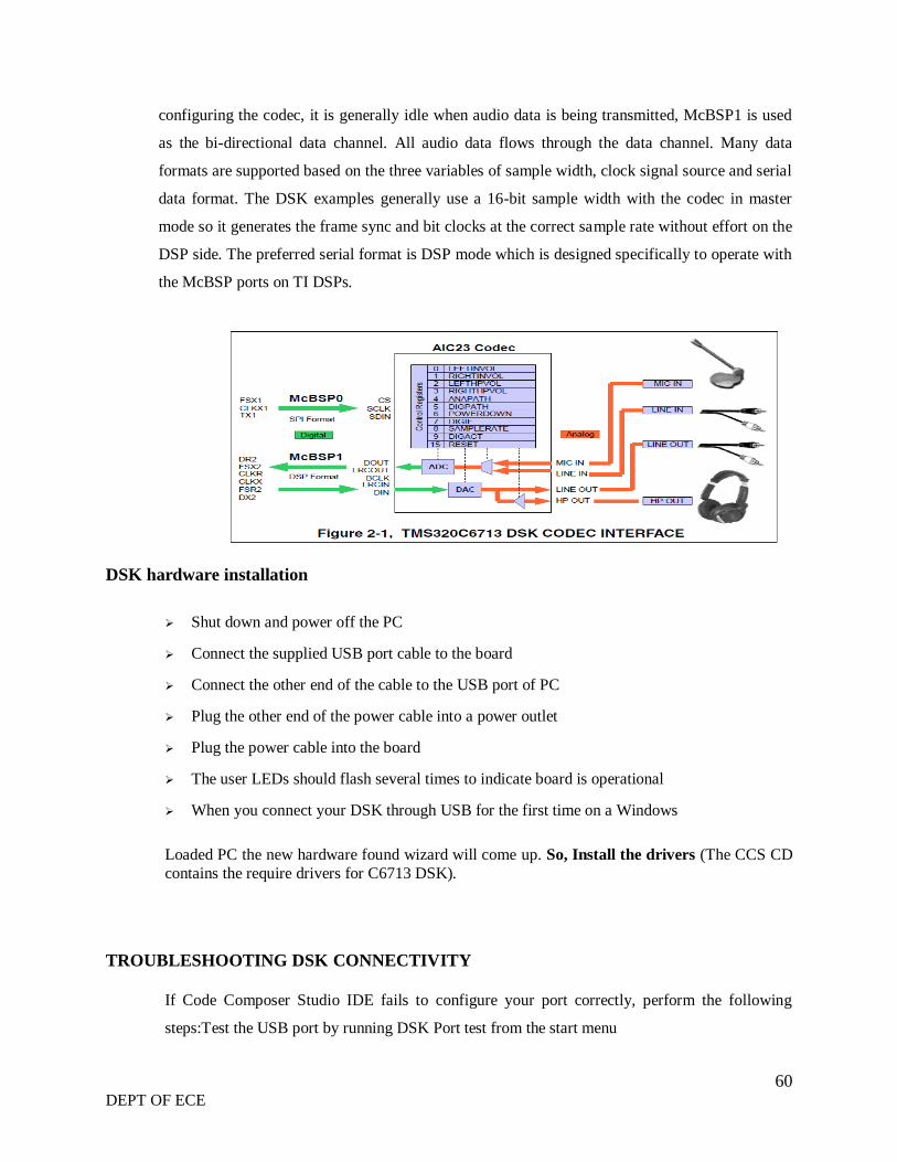
60 DEPT OF ECE
configuring the codec, it is generally idle when audio data is being transmitted, McBSP1 is used
as the bi-directional data channel. All audio data flows through the data channel. Many data
formats are supported based on the three variables of sample width, clock signal source and serial
data format. The DSK examples generally use a 16-bit sample width with the codec in master
mode so it generates the frame sync and bit clocks at the correct sample rate without effort on the
DSP side. The preferred serial format is DSP mode which is designed specifically to operate with
the McBSP ports on TI DSPs.
DSK hardware installation
Shut down and power off the PC
Connect the supplied USB port cable to the board
Connect the other end of the cable to the USB port of PC
Plug the other end of the power cable into a power outlet
Plug the power cable into the board
The user LEDs should flash several times to indicate board is operational
When you connect your DSK through USB for the first time on a Windows
Loaded PC the new hardware found wizard will come up. So, Install the drivers (The CCS CD
contains the require drivers for C6713 DSK).
TROUBLESHOOTING DSK CONNECTIVITY
If Code Composer Studio IDE fails to configure your port correctly, perform the following
steps:Test the USB port by running DSK Port test from the start menu
61 DEPT OF ECE
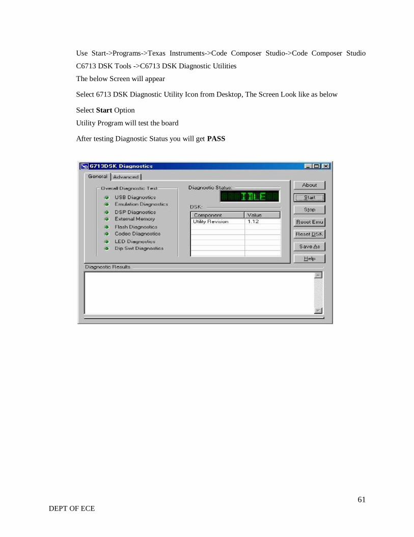
Use Start->Programs->Texas Instruments->Code Composer Studio->Code Composer Studio
C6713 DSK Tools ->C6713 DSK Diagnostic Utilities
The below Screen will appear
Select 6713 DSK Diagnostic Utility Icon from Desktop, The Screen Look like as below
Select Start Option
Utility Program will test the board
After testing Diagnostic Status you will get PASS
62 DEPT OF ECE
INTRODUCTION TO CODE COMPOSER STUDIO
Code Composer is the DSP industry's first fully integrated development environment(IDE) with
DSP-specific functionality. With a familiar environment liked MS-based C+, Code Composer
lets you edit, build, debug, profile and manage projects from asingle unified environment. Other
unique features include graphical signal analysis, injection/extraction of data signals via file I/O,
multi-processor debugging, automated testing and customization via a C-interpretive scripting
language and much more.
CODE COMPOSER FEATURES INCLUDE:
IDE
Debug IDE
Advanced watch windows
Integrated editor
File I/O, Probe Points, and graphical algorithm scope probes
Advanced graphical signal analysis
Interactive profiling
Automated testing and customization via scripting
Visual project management system
Compile in the background while editing and debugging
Multi-processor debugging
Help on the target DSP
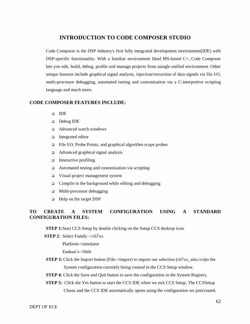
TO CREATE A SYSTEM CONFIGURATION USING A STANDARD
CONFIGURATION FILES:
STEP 1: Start CCS Setup by double clicking on the Setup CCS desktop icon.
STEP 2: Select Family ->c67xx
Platform->simulator
Endean‟s->little
STEP 3: Click the Import button (File->import) to import our selection (c67xx_sim.ccs)to the
System configuration currently being created in the CCS Setup window.
STEP 4: Click the Save and Quit button to save the configuration in the System Registry.
STEP 5: Click the Yes button to start the CCS IDE when we exit CCS Setup. The CCSSetup
Closes and the CCS IDE automatically opens using the configuration we justcreated.
63 DEPT OF ECE
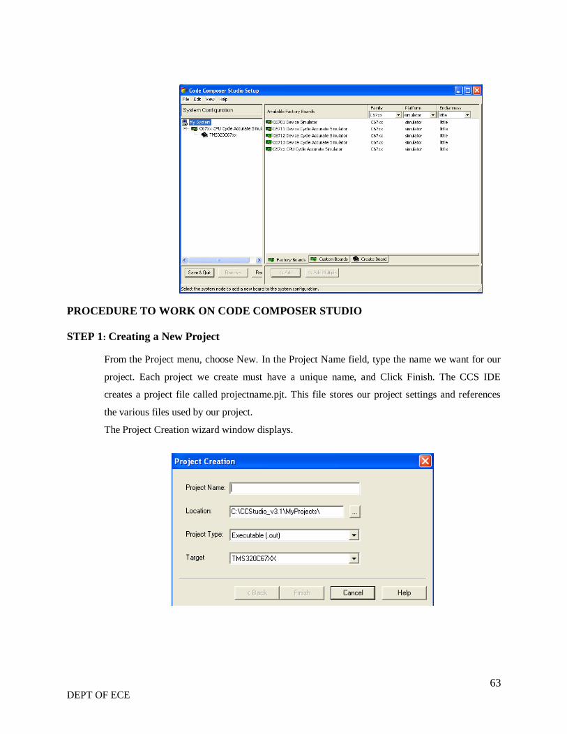
PROCEDURE TO WORK ON CODE COMPOSER STUDIO
STEP 1: Creating a New Project
From the Project menu, choose New. In the Project Name field, type the name we want for our
project. Each project we create must have a unique name, and Click Finish. The CCS IDE
creates a project file called projectname.pjt. This file stores our project settings and references
the various files used by our project.
The Project Creation wizard window displays.
64 DEPT OF ECE
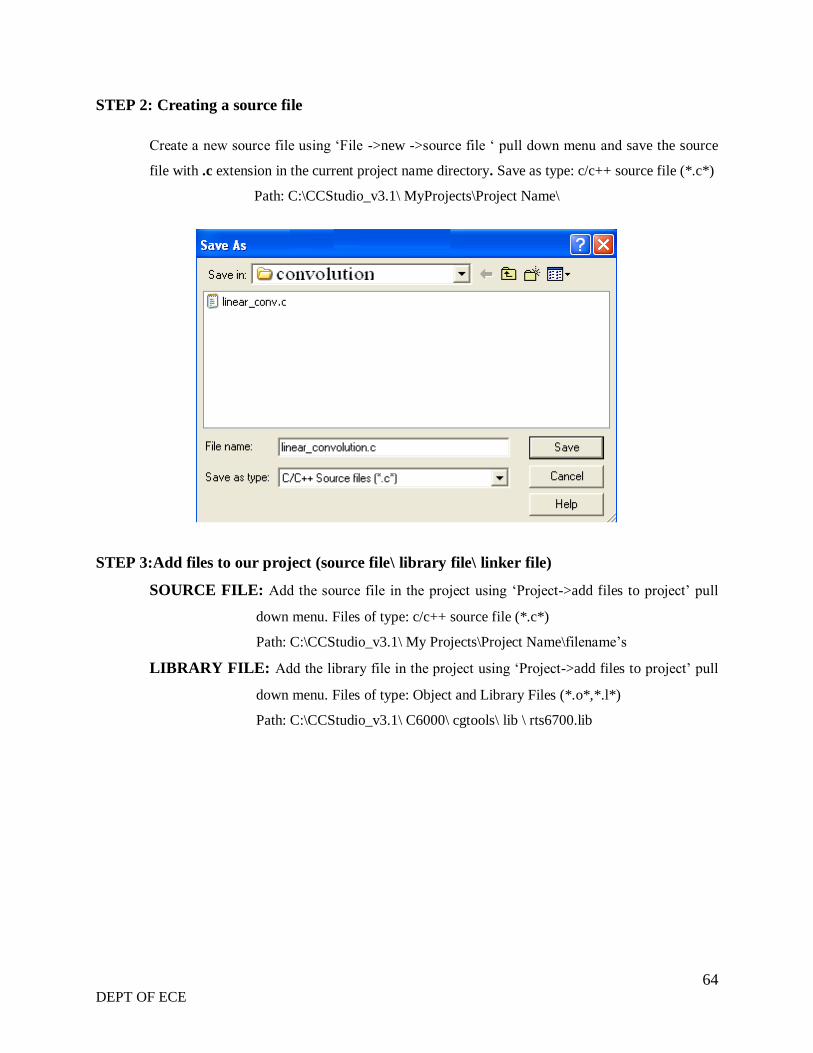
STEP 2: Creating a source file
Create a new source file using „File ->new ->source file „ pull down menu and save the source
file with .c extension in the current project name directory. Save as type: c/c++ source file (*.c*)
Path: C:\CCStudio_v3.1\ MyProjects\Project Name\
STEP 3:Add files to our project (source file\ library file\ linker file)
SOURCE FILE: Add the source file in the project using „Project->add files to project‟ pull
down menu. Files of type: c/c++ source file (*.c*)
Path: C:\CCStudio_v3.1\ My Projects\Project Name\filename‟s
LIBRARY FILE: Add the library file in the project using „Project->add files to project‟ pull
down menu. Files of type: Object and Library Files (*.o*,*.l*)
Path: C:\CCStudio_v3.1\ C6000\ cgtools\ lib \ rts6700.lib
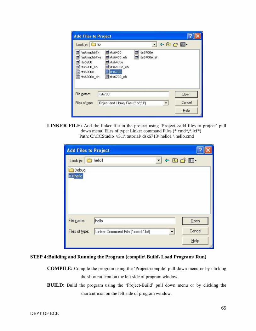
65 DEPT OF ECE
LINKER FILE: Add the linker file in the project using „Project->add files to project‟ pull down menu. Files of type: Linker command Files (*.cmd*,*.lcf*)
Path: C:\CCStudio_v3.1\ tutorial\ dsk6713\ hello1 \ hello.cmd
STEP 4:Building and Running the Program (compile\ Build\ Load Program\ Run)
COMPILE: Compile the program using the „Project-compile‟ pull down menu or by clicking
the shortcut icon on the left side of program window.
BUILD: Build the program using the „Project-Build‟ pull down menu or by clicking the
shortcut icon on the left side of program window.

66 DEPT OF ECE
LOAD PROGRAM:Load the program in program memory of DSP chip using the„File-load
program‟ pull down menu.Files of type:(*.out*)
Path: C:\CCStudio_v3.1\ MyProjects\Project Name\ Debug\ Project
ame.out
RUN: Run the program using the „Debug->Run‟ pull down menu or by clicking
theshortcut icon on the left side of program window.
STEP 5:observe output using graph
Choose View->Graph-> Time/Frequency. In The Graph Property Dialog, Change The Graph
Title, Start Address, And Acquisition Buffer Size, Display Data Size, Dsp Data Type, Auto
Scale, And Maximum Y- Value Properties To The Values.
67 DEPT OF ECE
EXPERIMENT No 1
N-POINT DFT
AIM:
Computation of N-point DFT of a Sequence Using DSK Code composer studio
EQUIPMENTS:
TMS 320C6713 Kit.
RS232 Serial Cable
Power Cord
Operating System – Windows XP
Software – CCStudio_v3.1
THEORY:
In this program the Discrete Fourier Transform (DFT) of a sequence x[n] is generated by using
the formula,
N-1
X (k) = Σ x(n) e-2πjk / N
Where, X(k) DFT of sequence x[n]
n=0
N represents the sequence length and it is calculated by using the command „length‟. The DFT
of any sequence is the powerful computational tool for performing frequency analysis of
discrete-time signals.
PROGRAM:
#include <stdio.h>
#include <math.h>
intN,k,n,i;
float pi=3.1416,sumre=0,sumim=0,out_real[8]={0.0},out_imag[8]={0.0};
int x[32];
void main(void)
{
printf("enter the length of the sequence\n");
scanf("%d",&N);
68 DEPT OF ECE
printf("\nenter the sequence\n");
for(i=0;i<N;i++)
scanf("%d",&x[i]);
for(k=0;k<N;k++)
{
sumre=0;
sumim=0;
for(n=0;n<N;n++)
{
sumre=sumre+x[n]*cos(2*pi*k*n/N);
sumim=sumim-x[n]*sin(2*pi*k*n/N);
}
out_real[k]=sumre;
out_imag[k]=sumim;
printf("DFT of the sequence:\n");
printf("x[%d]=\t%f\t+\t%fi\n",k,out_real[k],out_imag[k]);
}
}
PROCEDURE:
Open code composer studio, make sure the dsp kit is turned on.
Start a new project using „project-new „ pull down menu, save it in a separate
directory(d:11951a0xxx) with name dft.
Write the program and save it as dft.c
Add the source files dft.cto the project using „project->add files to project‟ pull down menu.
Add the linker command file hello.cmd.
(path: c:ccstudio_v3.1\tutorial\dsk6713\hello1\hello.cmd)
Add the run time support library file rts6700.lib.
(path: c:ccstudio_v3.1\c6000\cgtools\lib\rts6700.lib)
Compile the program using the „project-compile‟ pull down menu
Build the program using the „project-build‟ pull down menu
Load the program (dft.out) in program memory of dsp chip using the„file-load program‟ pull
down menu.
Debug-> run
69 DEPT OF ECE
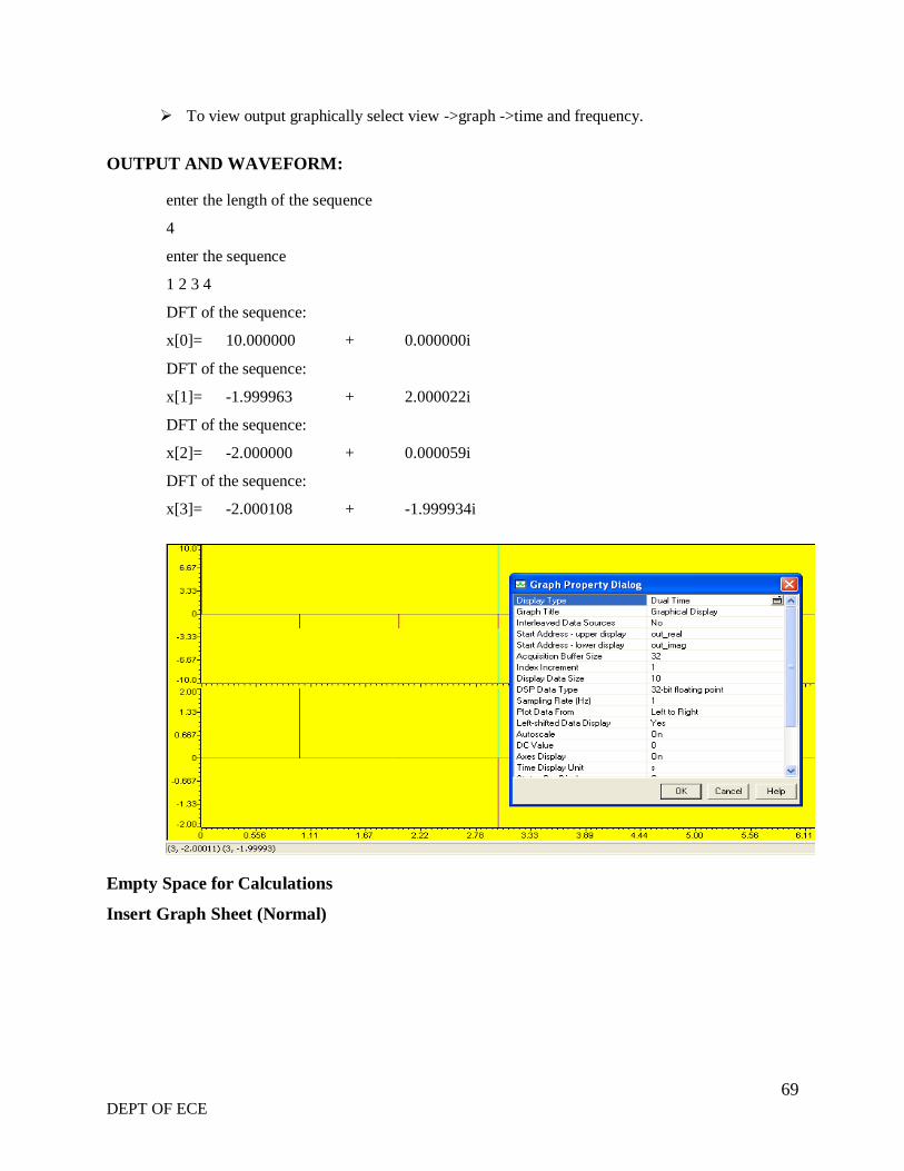
To view output graphically select view ->graph ->time and frequency.
OUTPUT AND WAVEFORM:
enter the length of the sequence
4
enter the sequence
1 2 3 4
DFT of the sequence:
x[0]= 10.000000 + 0.000000i
DFT of the sequence:
x[1]= -1.999963 + 2.000022i
DFT of the sequence:
x[2]= -2.000000 + 0.000059i
DFT of the sequence:
x[3]= -2.000108 + -1.999934i
Empty Space for Calculations
Insert Graph Sheet (Normal)
70 DEPT OF ECE
EXPERIMENT No 2
GENERATION OF SINE WAVE USING C6713 DSK
AIM:
To generate a real time sine wave using TMS320C6713 DSK
EQUIPMENTS:
TMS 320C6713 Kit.
RS232 Serial Cable
Power Cord
Operating System – Windows XP
Software – CCStudio_v3.1
PROCEDURE:
1. Connect CRO to the LINE OUT socket.
2. Now switch ON the DSK and bring up Code Composer Studio on PC
3. Create a new project with name sinewave.pjt
4. From File menu->New->DSP/BIOS Configuration->Select dsk6713.cdb and save it as
“ sinewave.cdb”
5. Add sinewave.cdb to the current project
6. Create a new source file and save it as sinewave.c
7. Add the source file sinewave.c to the project
8. Add the library file “dsk6713bsl.lib” to the project
( Path: C:\CCStudio\C6000\dsk6713\lib\dsk6713bsl.lib)
9. Copy files “dsk6713.h” and “dsk6713_aic23.h” to the Project folder
(Path: C:\CCStudio_v3.1\C6000\dsk6713\include)
10. Build (F7) and load the program to the DSP Chip ( File->Load Program(.out file))
11. Run the program (F5)
12. Observe the waveform that appears on the CRO screen and ccstudio simulator.
71 DEPT OF ECE
%% matlab code to generate the sine values of the look table
n=1:48;
x=sin(2*pi*n*1000/48000);
x1=round(x*2^15);
// c program for generation of sine wave using c6713 DSK
#include "sinewavecfg.h"
#include "dsk6713.h"
#include "dsk6713_aic23.h"
short loop=0;
short gain=1;
Int16 outbuffer[256];
const short BUFFERLENGTH=256;
inti=0;
DSK6713_AIC23_Config
config={0x0017,0x0017,0x00d8,0x00d8,0x0011,0x0000,0x0000,0x0043,0x0081,0x0001};
Int16 sine_table[48]={4277,8481,12540,16384,19948,23170,25997,28378,30274,31651,32488,
32766,32488,31651,30274,28378,25997,23170,19948,16384,12540,8481,4277,0,-4277,-8481,
-12540,-16384,-19948,-23170,-25997,-28378,-30274,-31651,-32488,-32766,-32488,-31651,
-30274,-28378,-25997,-23170,-19948,-16384,-12540,-8481,-4277,0};
Uint32 fs=DSK6713_AIC23_FREQ_48KHZ;
void main()
{
DSK6713_AIC23_CodecHandle hCodec;
DSK6713_init();
hCodec=DSK6713_AIC23_openCodec(0, &config);
DSK6713_AIC23_setFreq(hCodec, fs);
while(1)
{
outbuffer[i]=sine_table[loop];
while(!DSK6713_AIC23_write(hCodec, sine_table[loop])*gain);
i++;
if(i==BUFFERLENGTH) i=0;
if(++loop>47) loop=0;
}}

72 DEPT OF ECE
WAVEFORM:
a) output from code composer studio
b) output from the CRO
INSERT GRAPH SHEET (NORMAL)
73 DEPT OF ECE
EXPERIMENT No 3
FIR FILTER USING RECTANGULAR WINDOW (LOW PASS)
AIM:
To generate a real time fir filter through Rectangular window using TMS320C6713 DSK
EQUIPMENTS:
TMS 320C6713 Kit.
RS232 Serial Cable
Power Cord
Operating System – Windows XP
Software – CCStudio_v3.1
PROCEDURE:
1. Connect CRO to the LINE OUT sockets.
2. Now switch ON the DSK and bring up Code Composer Studio on PC
3. Create a new project with name sinewave.pjt
4. From File menu->New->DSP/BIOS Configuration->Select dsk6713.cdb and save it as
“ firfliter.cdb”
5. Add firfilter.cdb to the current project
6. Create a new source file and save it as firfilter.c
7. Add the source file firfilter.c to the project
8. Add the library file “dsk6713bsl.lib” to the project
(Path: C:\CCStudio\C6000\dsk6713\lib\dsk6713bsl.lib)
9. Copy files “dsk6713.h” and “dsk6713_aic23.h” to the Project folder
(Path: C:\CCStudio_v3.1\C6000\dsk6713\include)
10. Build (F7) and load the program to the DSP Chip ( File->Load Program(.out file))
11. Run the program (F5)
12. Observe the waveform that appears on the CRO screen and ccstudio simulator.
74 DEPT OF ECE
// c program for generation of fir filter using c6713 DSK
#include "firfiltercfg.h"
#include "dsk6713.h"
#include "dsk6713_aic23.h"
#include "stdio.h"
Floatfilter_coeff[]={-0.020203,-0.016567,0.009656,0.027335,0.011411,-0.023194,-
0.033672,0.000000,0.043293,0.038657,-0.025105,-0.082004,-0.041842,0.115971,0.303048,
0.386435,0.303048,0.115971,-0.041842,-0.082004,-0.025105,0.038657,0.043293,0.000000,-
0.033672,-0.023194,0.011411,0.027335,0.009656,-0.016567,-0.020203};//FIR Low pass
Rectangular Filter pass band range 0-1500Hz
DSK6713_AIC23_Config
config={0x0017,0x0017,0x00d8,0x00d8,0x0011,0x0000,0x0000,0x0043,0x0081,0x0001};
void main()
{
DSK6713_AIC23_CodecHandle hCodec;
Uint32 l_input, r_input,l_output, r_output;
DSK6713_init();
hCodec = DSK6713_AIC23_openCodec(0, &config);
DSK6713_AIC23_setFreq(hCodec, 1);
while(1)
{
while(!DSK6713_AIC23_read(hCodec, &l_input));
while(!DSK6713_AIC23_read(hCodec, &r_input));
l_output=(Int16)FIR_FILTER(&filter_coeff ,l_input);
r_output=l_output;
while(!DSK6713_AIC23_write(hCodec, l_output));
while(!DSK6713_AIC23_write(hCodec, r_output));
}
DSK6713_AIC23_closeCodec(hCodec);
}
signed int FIR_FILTER(float * h, signed int x)
{
inti=0;
signed long output=0;
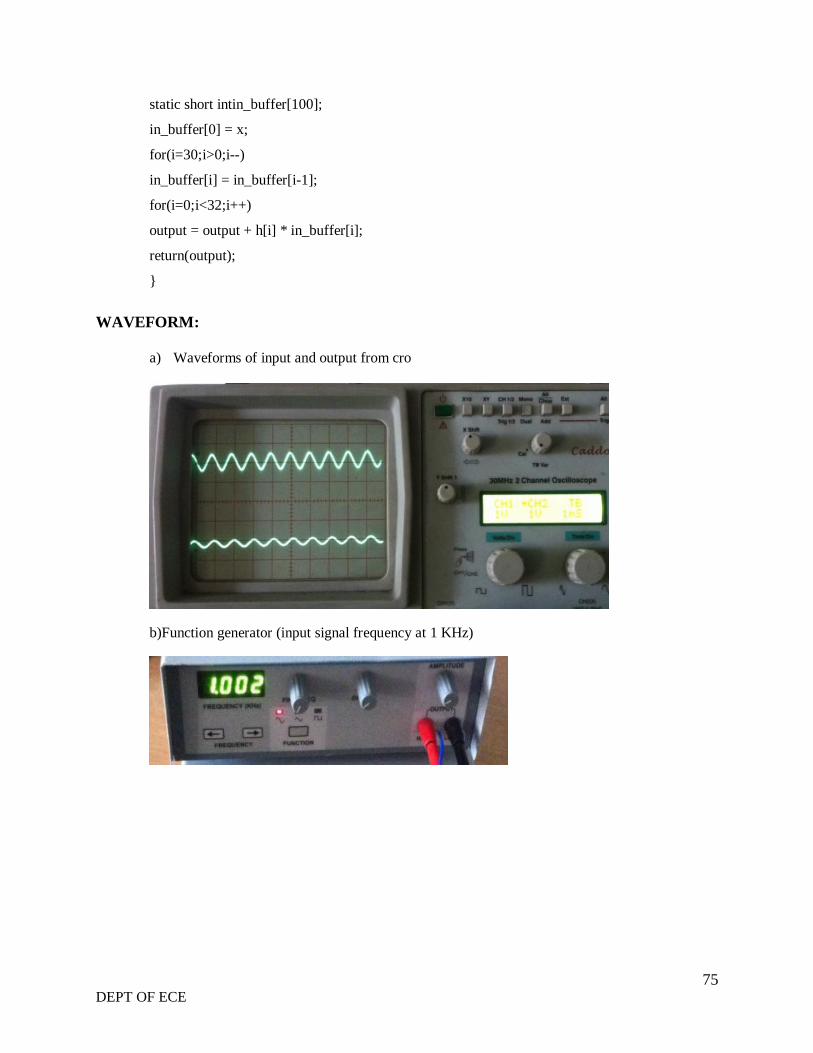
75 DEPT OF ECE
static short intin_buffer[100];
in_buffer[0] = x;
for(i=30;i>0;i--)
in_buffer[i] = in_buffer[i-1];
for(i=0;i<32;i++)
output = output + h[i] * in_buffer[i];
return(output);
}
WAVEFORM:
a) Waveforms of input and output from cro
b)Function generator (input signal frequency at 1 KHz)
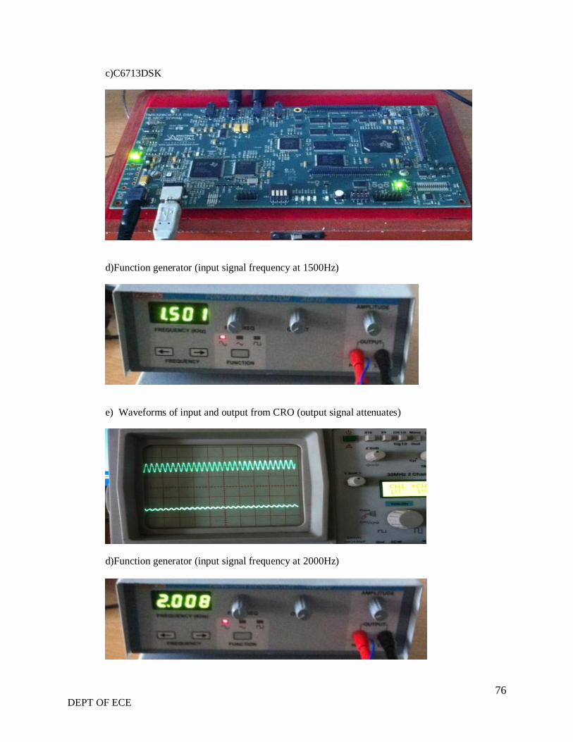
76 DEPT OF ECE
c)C6713DSK
d)Function generator (input signal frequency at 1500Hz)
e) Waveforms of input and output from CRO (output signal attenuates)
d)Function generator (input signal frequency at 2000Hz)
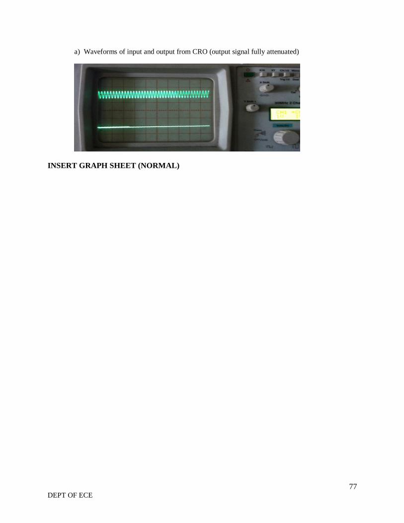
77 DEPT OF ECE
a) Waveforms of input and output from CRO (output signal fully attenuated)
INSERT GRAPH SHEET (NORMAL)
78 DEPT OF ECE
EXPERIMENT No 4
FIR FILTER USING KAISER WINDOW (HIGH PASS)
AIM:
To generate a real time fir filter through KaiserWindow using TMS320C6713 DSK
EQUIPMENTS:
TMS 320C6713 Kit.
RS232 Serial Cable
Power Cord
Operating System – Windows XP
Software – CCStudio_v3.1
PROCEDURE:
1. Connect CRO to the LINE OUT sockets.
2. Now switch ON the DSK and bring up Code Composer Studio on PC
3. Create a new project with name sinewave.pjt
4. From File menu->New->DSP/BIOS Configuration->Select dsk6713.cdb and save it as
“firfliter_kaiser.cdb”
5. Add firfilter.cdb to the current project
6. Create a new source file and save it as firfilter_kaiser.c
7. Add the source file firfilter_kaiser.c to the project
8. Add the library file “dsk6713bsl.lib” to the project
(Path: C:\CCStudio\C6000\dsk6713\lib\dsk6713bsl.lib)
9. Copy files “dsk6713.h” and “dsk6713_aic23.h” to the Project folder
(Path: C:\CCStudio_v3.1\C6000\dsk6713\include)
10. Build (F7) and load the program to the DSP Chip (File->Load Program (.out file))
11. Run the program (F5)
12. Observe the waveform that appears on the CRO screen and ccstudio simulator.
79 DEPT OF ECE
// c program for generation of fir filter using c6713 DSK
#include "firfilter_kaisercfg.h"
#include "dsk6713.h"
#include "dsk6713_aic23.h"
#include "stdio.h"
float filter_coeff[]={0.000000,-0.000138,-0.000611,-0.001345,-0.001607, 0.000000, 0.004714,
0.012033,0.018287,0.016731,0.000000,-0.035687,-0.086763,-0.141588,-0.184011,0.800005, -
0.184011,-0.141588,-0.086763,-0.035687,0.000000,0.016731,0.018287,0.012033,0.004714, -
0.000000,-0.001607,-0.001345,-0.000611,-0.000138,0.000000};//FIR High pass Kaiser filter pass band
range 800Hz-3.5KHz
void main()
{
DSK6713_AIC23_CodecHandle hCodec;
Uint32 l_input, r_input,l_output, r_output;
DSK6713_init();
hCodec = DSK6713_AIC23_openCodec(0, &config);
DSK6713_AIC23_setFreq(hCodec, 1);
while(1)
{
while(!DSK6713_AIC23_read(hCodec, &l_input));
while(!DSK6713_AIC23_read(hCodec, &r_input));
l_output=(Int16)FIR_FILTER(&filter_coeff ,l_input);
r_output=l_output;
while(!DSK6713_AIC23_write(hCodec, l_output));
while(!DSK6713_AIC23_write(hCodec, r_output));
}
DSK6713_AIC23_closeCodec(hCodec);
}
signed int FIR_FILTER(float * h, signed int x)
{
inti=0;
signed long output=0;
static short intin_buffer[100];
in_buffer[0] = x;
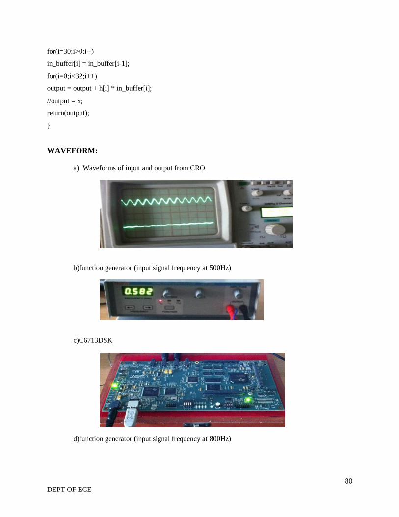
80 DEPT OF ECE
for(i=30;i>0;i--)
in_buffer[i] = in_buffer[i-1];
for(i=0;i<32;i++)
output = output + h[i] * in_buffer[i];
//output = x;
return(output);
}
WAVEFORM:
a) Waveforms of input and output from CRO
b)function generator (input signal frequency at 500Hz)
c)C6713DSK
d)function generator (input signal frequency at 800Hz)
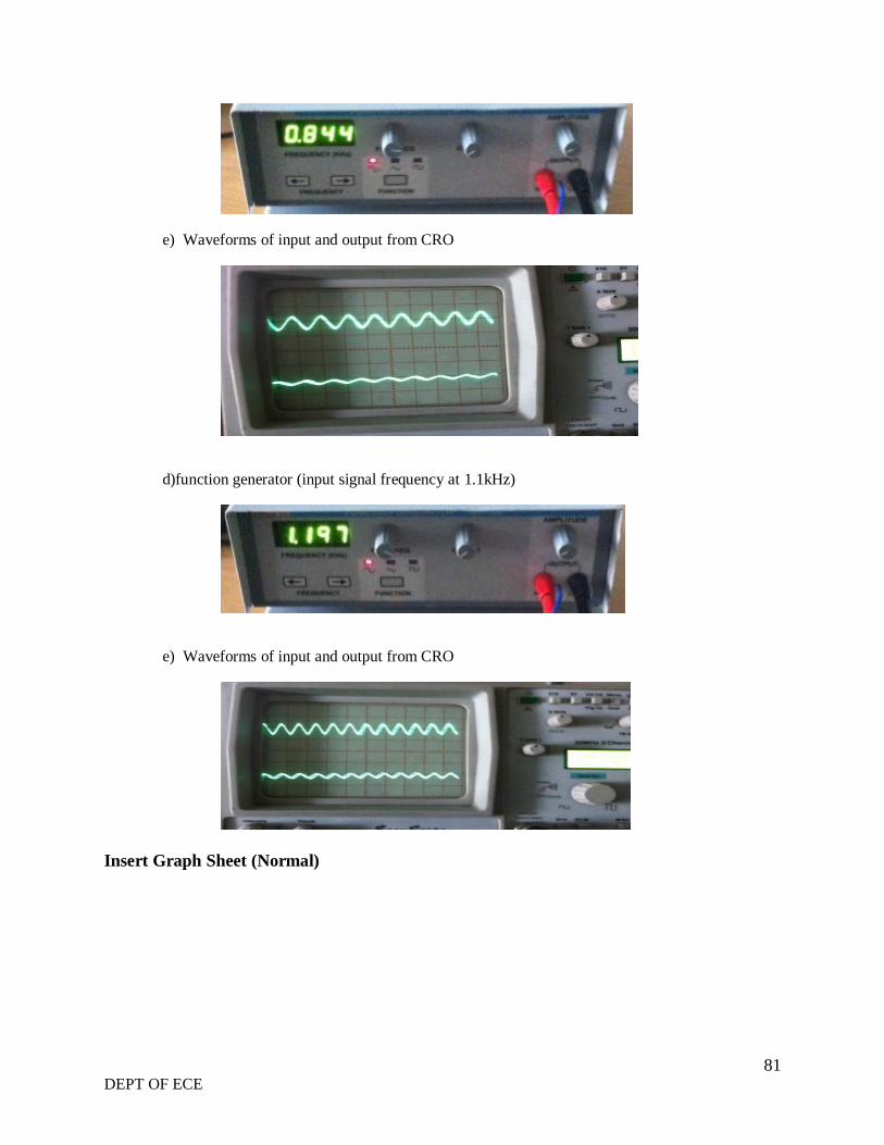
81 DEPT OF ECE
e) Waveforms of input and output from CRO
d)function generator (input signal frequency at 1.1kHz)
e) Waveforms of input and output from CRO
Insert Graph Sheet (Normal)
82 DEPT OF ECE
EXPERIMENT No 5
IIR FILTER USING BUTTERWORTH APPROXIMATION (LOW PASS)
AIM:
To generate a real time iir filter through Butterworth approximation using TMS320C6713 DSK
EQUIPMENTS:
TMS 320C6713 Kit.
RS232 Serial Cable
Power Cord
Operating System – Windows XP
Software – CCStudio_v3.1
PROCEDURE:
1. Connect CRO to the LINE OUT socket.
2. Now switch ON the DSK and bring up Code Composer Studio on PC
3. Create a new project with name sinewave.pjt
4. From File menu->New->DSP/BIOS Configuration->Select dsk6713.cdb and save it as
“iirfliter.cdb”
5. Add firfilter.cdb to the current project
6. Create a new source file and save it as iirfilter.c
7. Add the source file iirfilter.c to the project
8. Add the library file “dsk6713bsl.lib” to the project
(Path: C:\CCStudio\C6000\dsk6713\lib\dsk6713bsl.lib)
9. Copy files “dsk6713.h” and “dsk6713_aic23.h” to the Project folder
(Path: C:\CCStudio_v3.1\C6000\dsk6713\include)
10. Build (F7) and load the program to the DSP Chip ( File->Load Program(.out file))
11. Run the program (F5)
12. Observe the waveform that appears on the CRO screen and ccstudio simulator.
83 DEPT OF ECE
// c program for generation of iir filter using c6713 DSK
#include "iirfiltercfg.h"
#include "dsk6713.h"
#include "dsk6713_aic23.h"
#include "stdio.h"
const signed intfilter_coeff [ ] = {15241,15241,15241,32761,10161,7877};
//IIR_BUTERWORTH_LP FILTER pass band range 0-8kHz
DSK6713_AIC23_Config
config={0x0017,0x0017,0x00d8,0x00d8,0x0011,0x0000,0x0000,0x0043,0x0081,0x0001};
void main()
{
DSK6713_AIC23_CodecHandle hCodec;
Uint32 l_input, r_input,l_output, r_output;
DSK6713_init();
hCodec = DSK6713_AIC23_openCodec(0, &config);
DSK6713_AIC23_setFreq(hCodec, 3);
while(1)
{
while(!DSK6713_AIC23_read(hCodec, &l_input));
while(!DSK6713_AIC23_read(hCodec, &r_input));
l_output=IIR_FILTER(&filter_coeff ,l_input);
r_output=l_output;
while(!DSK6713_AIC23_write(hCodec, l_output));
while(!DSK6713_AIC23_write(hCodec, r_output));
}
DSK6713_AIC23_closeCodec(hCodec);
}
signed int IIR_FILTER(const signed int * h, signed int x1)
{
static signed int x[6] = {0,0,0,0,0,0};
static signed int y[6] = {0,0,0,0,0,0};
int temp=0;
temp = (short int)x1;
x[0] = (signed int) temp;

84 DEPT OF ECE
temp = ( (int)h[0] * x[0]);
temp += ( (int)h[1] * x[1]);
temp += ( (int)h[1] * x[1]);
temp += ( (int)h[2] * x[2]);
temp -= ( (int)h[4] * y[1]);
temp -= ( (int)h[4] * y[1]);
temp -= ( (int)h[5] * y[2]);
temp >>=15;
if ( temp > 32767 )
{
temp = 32767;
}
else if ( temp < -32767)
{
temp = -32767;
}
y[0] = temp;
y[2] = y[1];
y[1] = y[0];
x[2] = x[1];
x[1] = x[0];
return (temp<<2);
}
RESULT:
a) Waveforms of input and output from CRO
b)function generator (input signal frequency at 1KHz)
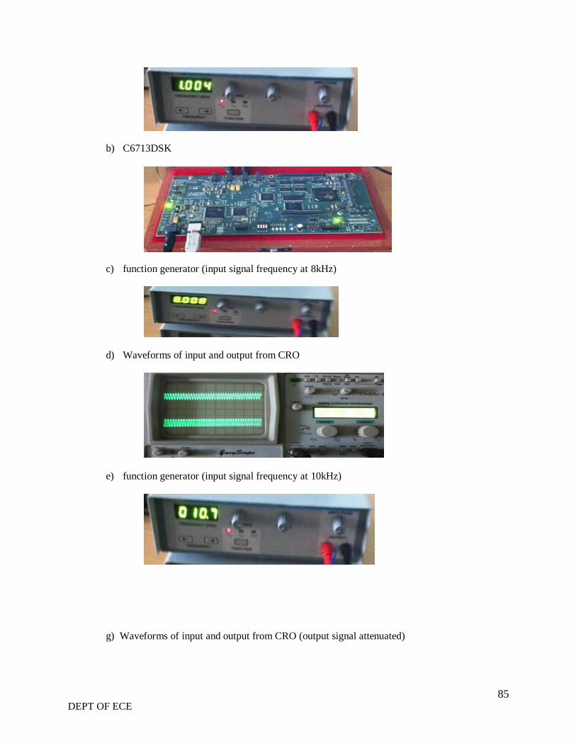
85 DEPT OF ECE
b) C6713DSK
c) function generator (input signal frequency at 8kHz)
d) Waveforms of input and output from CRO
e) function generator (input signal frequency at 10kHz)
g) Waveforms of input and output from CRO (output signal attenuated)
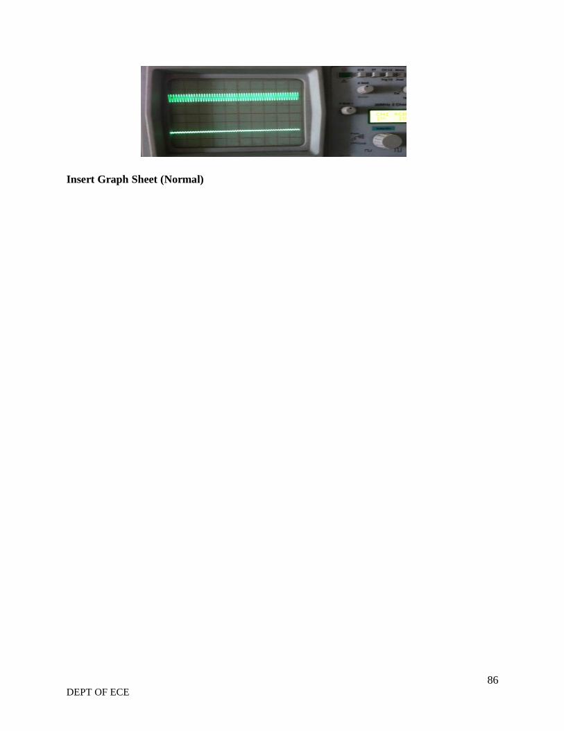
86 DEPT OF ECE
Insert Graph Sheet (Normal)

87 DEPT OF ECE
CONTENT BEYOND SYLLABI
88 DEPT OF ECE
EXPERIMENT No 1
LINEAR CONVOLUTION
AIM:
Verify the linear convolution operation Using DSK Code composer studio
EQUIPMENTS:
TMS 320C6713 Kit.
RS232 Serial Cable
Power Cord
Operating System – Windows XP
Software – CCStudio_v3.1
THEORY:
Convolution is a formal mathematical operation, just as multiplication, addition, and integration.
Addition takes two numbers and produces a third number, while convolution takes two signals
and produces a third signal. Convolution is used in the mathematics of many fields, such as
probability and statistics. In linear systems, convolution is used to describe the relationship
between three signals of interest: the input signal, the impulse response, and the output signal.
10)()()(
1
0
Nnknhkxny
N
k
In this equation, x(k), h(n-k) and y(n) represent the input to and output from the system at time
n. Here we could see that one of the input is shifted in time by a value every time it is multiplied
with the other input signal. Linear Convolution is quite often used as a method of implementing
filters of various types.
PROGRAM:
// Linear convolution program in c language using ccstudio
#include<stdio.h>
int x[15],h[15],y[15];
main()
{
inti,j,m,n;

89 DEPT OF ECE
printf("\n enter the length of first sequence m:");
scanf("%d",&m);
printf("\n enter the length of second sequence n:");
scanf("%d",&n);
printf("enter values for i/p sequence x(n):\n");
for(i=0;i<m;i++)
scanf("%d",&x[i]);
printf("enter values for i/p sequence h(n): \n");
for(i=0;i<n; i++)
scanf("%d",&h[i]);
// padding of zeros
for(i=m;i<=m+n-1;i++)
x[i]=0;
for(i=n;i<=m+n-1;i++)
h[i]=0;
/* convolution operation */
for(i=0;i<m+n-1;i++)
{
y[i]=0;
for(j=0;j<=i;j++)
{
y[i]=y[i]+(x[j]*h[i-j]);
}
}
//displaying the o/p
for(i=0;i<m+n-1;i++)
printf("\n the value of output y[%d]=%d\t",i,y[i]);
}
PROCEDURE:
Open Code Composer Studio; make sure the DSP kit is turned on.
Start a new project using „Project-new „pull down menu, save it in a separate directory (D:
11951A0xxx) with name linear convolution.
Write the program and save it as linearconv.c

90 DEPT OF ECE
Add the source files linearconv.cto the project using „Project->add files to project‟ pull down
menu.
Add the linker command file hello.cmd.
(Path: C:CCstudio_V3.1\tutorial\dsk6713\hello1\hello.cmd)
Add the run time support library file rts6700.lib.
(Path: C:CCstudio_v3.1\c6000\cgtools\lib\rts6700.lib)
Compile the program using the „Project-compile‟ pull down menu
Build the program using the „Project-Build‟ pull down menu
Load the program (linearconv.out) in program memory of DSP chip using the „File-load
program‟ pull down menu.
Debug-> Run
To View output graphically Select view ->graph ->time and frequency.
OUTPUT AND WAVEFORM:
Enter first sequence length m: 4
Enter second sequence length n: 3
Enter i/p sequence for x (n):
1 2 3 4
Enter i/p sequence for h (n):
2 3 1
Output (Linear Convolution) sequence is:
y[0]=2 y[1]=7 y[2]=13 y[3]=19 y[4]=15 y[5]=4
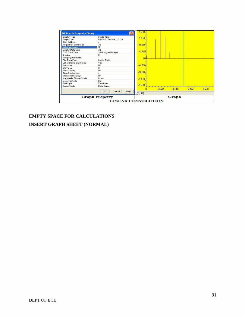
91 DEPT OF ECE
EMPTY SPACE FOR CALCULATIONS
INSERT GRAPH SHEET (NORMAL)
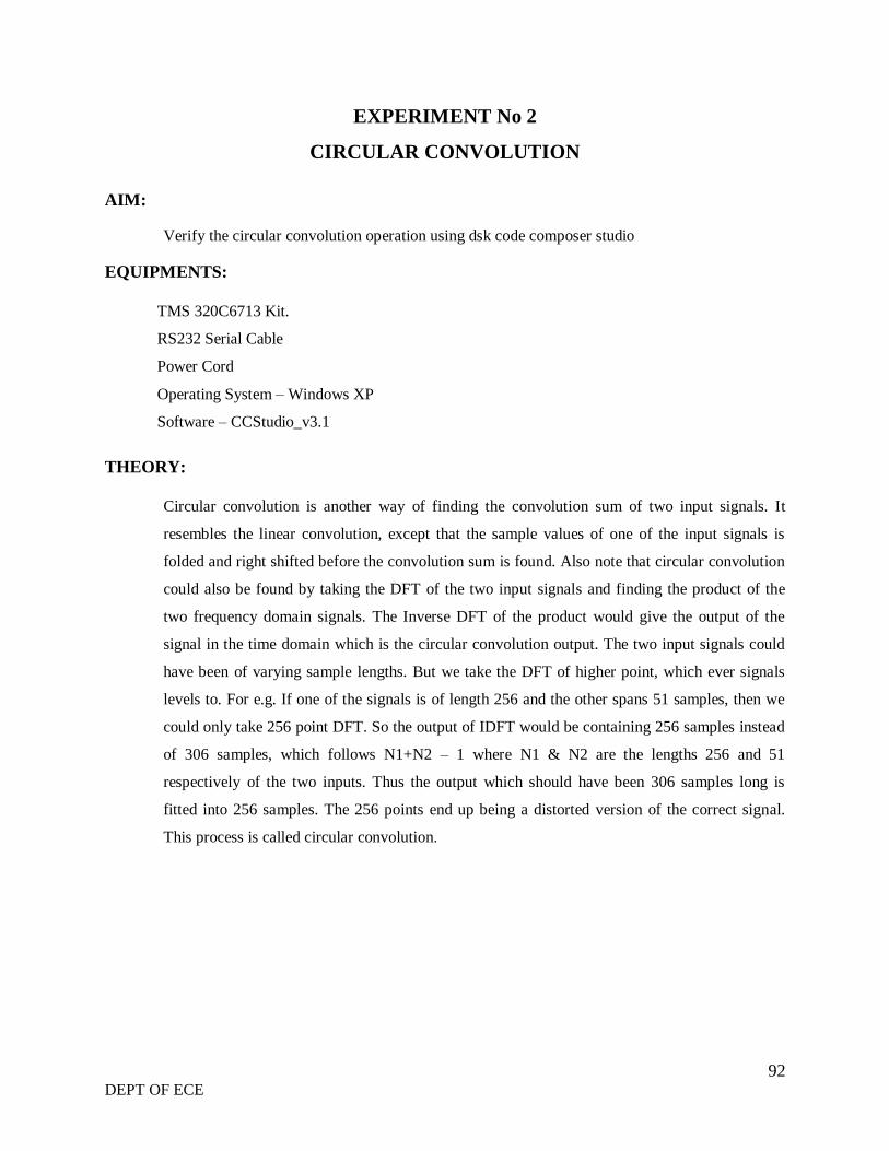
92 DEPT OF ECE
EXPERIMENT No 2
CIRCULAR CONVOLUTION
AIM:
Verify the circular convolution operation using dsk code composer studio
EQUIPMENTS:
TMS 320C6713 Kit.
RS232 Serial Cable
Power Cord
Operating System – Windows XP
Software – CCStudio_v3.1
THEORY:
Circular convolution is another way of finding the convolution sum of two input signals. It
resembles the linear convolution, except that the sample values of one of the input signals is
folded and right shifted before the convolution sum is found. Also note that circular convolution
could also be found by taking the DFT of the two input signals and finding the product of the
two frequency domain signals. The Inverse DFT of the product would give the output of the
signal in the time domain which is the circular convolution output. The two input signals could
have been of varying sample lengths. But we take the DFT of higher point, which ever signals
levels to. For e.g. If one of the signals is of length 256 and the other spans 51 samples, then we
could only take 256 point DFT. So the output of IDFT would be containing 256 samples instead
of 306 samples, which follows N1+N2 – 1 where N1 & N2 are the lengths 256 and 51
respectively of the two inputs. Thus the output which should have been 306 samples long is
fitted into 256 samples. The 256 points end up being a distorted version of the correct signal.
This process is called circular convolution.
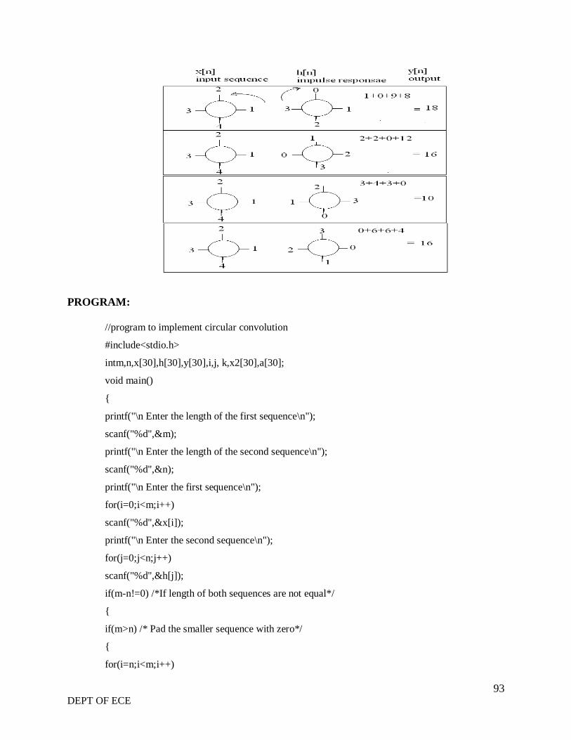
93 DEPT OF ECE
PROGRAM:
//program to implement circular convolution
#include<stdio.h>
intm,n,x[30],h[30],y[30],i,j, k,x2[30],a[30];
void main()
{
printf("\n Enter the length of the first sequence\n");
scanf("%d",&m);
printf("\n Enter the length of the second sequence\n");
scanf("%d",&n);
printf("\n Enter the first sequence\n");
for(i=0;i<m;i++)
scanf("%d",&x[i]);
printf("\n Enter the second sequence\n");
for(j=0;j<n;j++)
scanf("%d",&h[j]);
if(m-n!=0) /*If length of both sequences are not equal*/
{
if(m>n) /* Pad the smaller sequence with zero*/
{
for(i=n;i<m;i++)
94 DEPT OF ECE
h[i]=0;
n=m;
}
for(i=m;i<n;i++)
x[i]=0;
m=n;
}
y[0]=0;
a[0]=h[0];
for(j=1;j<n;j++) /*folding h(n) to h(-n)*/
a[j]=h[n-j];
/*Circular convolution*/
for(i=0;i<n;i++)
y[0]+=x[i]*a[i];
for(k=1;k<n;k++)
{
y[k]=0;
/*circular shift*/
for(j=1;j<n;j++)
x2[j]=a[j-1];
x2[0]=a[n-1];
for(i=0;i<n;i++)
{
a[i]=x2[i];
y[k]+=x[i]*x2[i];
}
}
//displaying the result
printf("\n The circular convolution is: \n");
for(i=0;i<n;i++)
printf("%d \t",y[i]);
}
95 DEPT OF ECE
PROCEDURE:
Open Code Composer Studio, make sure the DSP kit is turned on.
Start a new project using „Project-new „ pull down menu, save it in a separate
directory(D:11951A0xxx) with name circular convolution.
Write the program and save it as circularconv.c
Add the source files circularconv.cto the project using „Project->add files to project‟ pull
down menu.
Add the linker command file hello.cmd.
(Path: C:CCstudio_V3.1\tutorial\dsk6713\hello1\hello.cmd)
Add the run time support library file rts6700.lib.
(Path: C:CCstudio_v3.1\c6000\cgtools\lib\rts6700.lib)
Compile the program using the „Project-compile‟ pull down menu
Build the program using the „Project-Build‟ pull down menu
Load the program (circularconv.out) in program memory of DSP chip using the„File-load
program‟ pull down menu.
Debug-> Run
To View output graphically Select view ->graph ->time and frequency.
OUTPUT AND WAVEFORM:
Enter the length of the first sequence 4
Enter the length of the second sequence 3 Enter the first sequence
1 2 3 4
Enter the second sequence 1 2 3
The circular convolution is
18 16 10 16
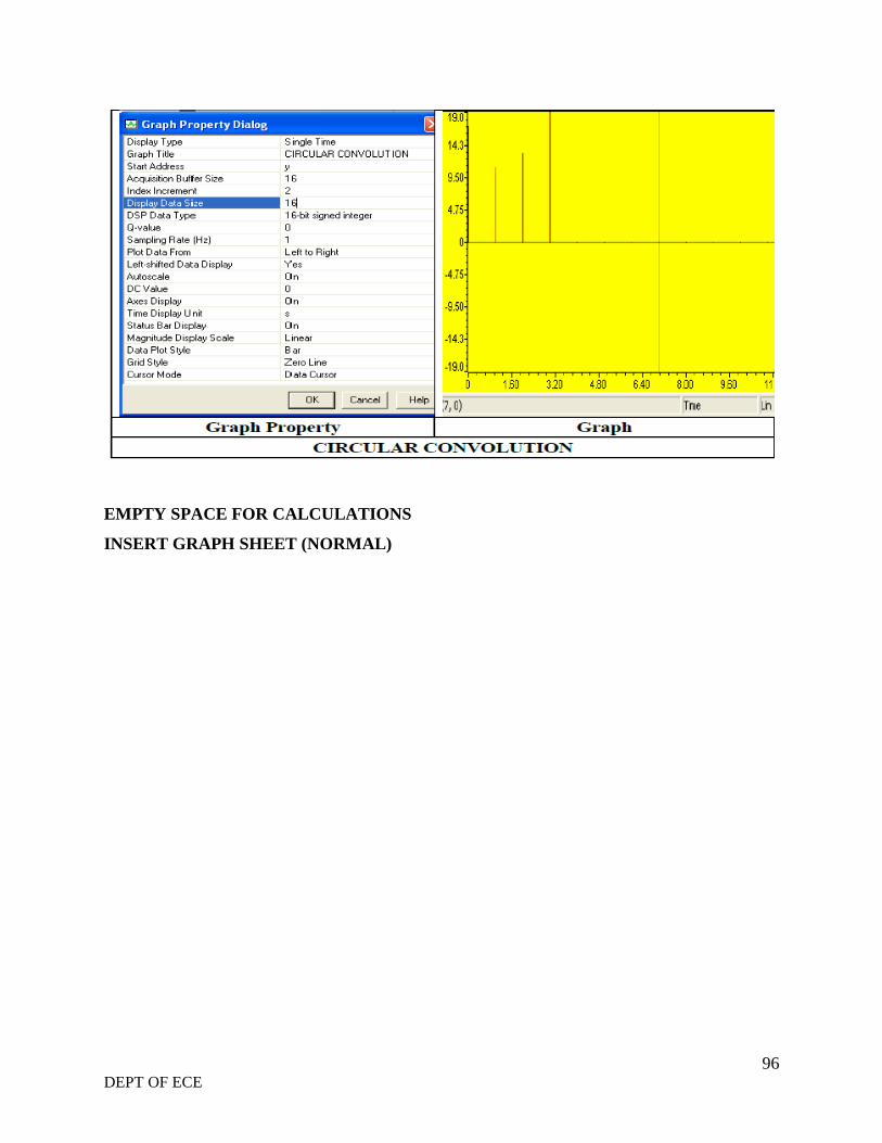
96 DEPT OF ECE
EMPTY SPACE FOR CALCULATIONS
INSERT GRAPH SHEET (NORMAL)
97 DEPT OF ECE
Annexure –I
VIVA QUESTIONS
GENERATION OF SINUSOIDAL SIGNAL QUESTIONS
1. What is the difference between sin & cos signals?
2. What is meant by signal?
3. What is the difference between time domain & frequency domain signal?
4. What is the difference between periodic & a periodic signal.
5. What is the difference between orthogonal and orthonormal signals?
6. What is the need for Fourier series & Fourier transform?
7. What is the difference between discrete & digital signals?
8. What is the difference between even signal & odd signal?
9. What is the difference between power signal & energy signal?
10. What is the difference between amplitude scaling & time scaling of a signal?
11. What is the difference between deterministic & random signal?
LINEAR CONVOLUTION QUESTIONS
1. What is the requirement for convolution?.
2. What is the difference between convolution & correlation?
3. What is meant by impulse response?
4. Is it possible to represent any discrete time signal in terms of impulses? If yes,
represent by using example.
5. Draw the h(2n-k) & h(n-2k) for the following sequenceh(n) = { 4 3 2 1} assume (i) k=
3 (ii) k =5.
6. Write the expressions for LTI system convolution formula & causal LTI
systemconvolution formula.
7. What us the length of linear convolution if length of input & impulse responsesare N1
& N2 respectively?
8. What is the difference between continuous and discrete convolution?

98 DEPT OF ECE
CIRCULAR CONVOLUTION QUESTIONS
1. Why we need circular convolution?
2. What is the difference between circular & linear convolution?
3. What is the length of output sequence after circular convolution if the lengths ofinput &
impulse responses are M1 & M2 respectively?
4. State the circular convolution property of DFT?
5. Where we required convolution property?
6. What does zero padding mean? Where we required this concept?
7. What is difference between linear shifting & circular shifting of signal? Show
withexample.
8. What is difference between linear & circular folding of signal? Show withexample.
9. What is the advantage with sectioned convolution?
FAST FOURIER TRANSFORM QUESTION
1. What is the difference between continuous time & discrete time Fourier transform?
2. What is the condition for convergence of Fourier transform?
3. What is the difference between discrete Time Fourier Transform (DTFT)& DFT?
4. What is the difference between Z transform & DFT?
5. State convolution property of the DFT? Where we could use the convolutionproperty?
6. State Parseval‟stheorem.
7. State correlation property of the DFT.?
8. What is the difference between radix 2 & radix4 FFT algorithms?
9. Why we need FFT?.
10. What is the difference between decimation in time (DIT FFT) & Decimation
infrequency(DIFFFT) algorithms?
11. What is meant by „in-place‟ computation in DIF & DIF algorithms?
12. Which properties are used in FFT to reduce no of computations?
FIR FILTER QUESTIONS
1. What are the advantages of FIR as compared to IIR?
2. How many types of FIR design methods are used in real time?.
3. What is meant by Gibbs Phenomenon? Where we found such type of effect in FIR
Filters?

99 DEPT OF ECE
4. What are the advantages& disadvantages of Rectangular window FIR filter as
Compared to remaining window techniques?
5. Which window technique having less peak amplitude of side lobe as compared toall?
6. What do you understand by linear phase responce?
7. To design all types of filters what would be the expected impulse response?
8. What are the properties of FIR filter?.
9. How the zeros in FIR filter is located?
10. What are the desirable characteristics of the window?
11. What are the specifications required to design filter
IIR FILTER QUESTIONS
1. What is meant by IIR filter?
2. What is the difference between recursive & non-recursive systems?
3. Write the difference equation for IIR system.
4. What are the mapping techniques in IIR filter design? Discuss the advantage
&disadvantages of them.
5. What are IIR analog filters? What are the advantages & disadvantages of them?
6. What is the disadvantage in impulse invariance method?
7. What does warping effect mean? Where we found this effect? How can weeliminate
warping effect?
8. Explain the pole mapping procedure of Impulse invariant & bilinear
transformationmethod.
9. For given same specification which difference we found in Butter worth &chebyshev
filter.
10. What is the difference between type I & type II chebyshev filters?.
11. Where the poles are located for Butter worth &chedbyshev filters?
12. What is meant by spectral transformation?
13. Why we need spectral transformation in IIR filter?
POWER SPECTRUM DENSITY QUESTION
1. What is the difference between correlation & auto correlation function?
2. What is the difference between PSD & ESD?
3. What is the unit for energy density spectrum?

100 DEPT OF ECE
4. What is the formula for PSD of a function?
5. “Same power density spectrum signals always have same magnitude &phase
spectrums” Is above statement true (or) False: Justify your answer.
6. If we know the impulse response of the system, the How can you find output
signalpower density from the input signal?
7. What is the unit for power density spectrum?
8. What is the relation between auto correlation & PSD of a function?
DSP PROCESSORS QUESTIONS
1. How many types of DSP processors are available in the market?
2. TMS 320C6X, „C‟ stands for what?
3. What are the features of TMS 320C6X processor?
4. What is meant by VLIW architecture? Why we required in DSP processor?
5. How many functional units are in TMS 320C6X DSP processor?
6. What is meant by Circular addressing mode how is it useful for DSP?
7. Which instruction is used to move 16 bit constant in to the upper bits of a register?
8. What is the difference between Von Neumann architecture & Harvardarchitecture?
9. Which architecture is used in DSP processor?
10. How many instructions can we execute per cycle in TMS320C6X DSP processor?
11. What are the applications for the TMS320 DSP‟s?
12. Which soft ware tool is required to compile and run the DSP assembly program?
13. What is the difference between full version Code composer studio &DSK CCS?


![ECE-V-DIGITAL SIGNAL PROCESSING [10EC52] …vtusolution.in/.../digital-signal-processing-10ec52.pdfDigital vtusolution.in Signal Processing 10EC52 TEXT BOOK: 1. DIGITAL SIGNAL PROCESSING](https://img.pdfslide.us/doc/110x75/5afe42bb7f8b9a256b8ccd2e/ece-v-digital-signal-processing-10ec52-signal-processing-10ec52-text-book.jpg)


![Ece v Digital Signal Processing [10ec52] Notes](https://img.pdfslide.us/doc/110x75/552bbbc74a7959dc7c8b4588/ece-v-digital-signal-processing-10ec52-notes.jpg)

![ECE-V-DIGITAL SIGNAL PROCESSING [10EC52]-NOTES.pdf](https://img.pdfslide.us/doc/110x75/56d6cbe71a28ab30169caa7d/ece-v-digital-signal-processing-10ec52-notespdf.jpg)


![Ece v Digital Signal Processing [10ec52] Solution](https://img.pdfslide.us/doc/110x75/552bbc224a7959cd7c8b45a7/ece-v-digital-signal-processing-10ec52-solution.jpg)