Embed Size (px)
Citation preview
DSP Course Introduction
Digital Signal Processing
Course Introduction
D. Richard Brown III
Meeting 1
D. Richard Brown III Meeting 1 1 / 48
DSP Course Introduction
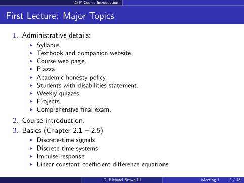
First Lecture: Major Topics
1. Administrative details: Syllabus. Textbook and companion website. Course web page. Piazza. Academic honesty policy. Students with disabilities statement. Weekly quizzes. Projects. Comprehensive final exam.
2. Course introduction.
3. Basics (Chapter 2.1 – 2.5) Discrete-time signals Discrete-time systems Impulse response Linear constant coefficient difference equations
D. Richard Brown III Meeting 1 2 / 48
DSP Course Introduction
Why No Homework?
I have found almost no value in collecting and grading homework.
Homework grades are a poor assessment of student understanding. Inmy experience, homework grades are almost entirely uncorrelated tofinal course grades.
Academic honesty problems.
Student focus is often on handing something in rather than reallylearning the material.
You still need to do problems to understand this material. I will provideseveral suggested problems and solutions each week for you to use forpractice. You are encouraged to collaborate!
D. Richard Brown III Meeting 1 3 / 48
DSP Course Introduction
Why Weekly Quizzes?
The traditional midterm/final format encourages “cramming”. There is alot of research that shows cramming, while an efficient use of time forstudying for exams, leads to very poor long-term retention of the material.
High-stakes midterm/final exams penalize students who have one bad day.
Weekly quizzes: Immediate feedback for instructor. Students can have abad day and still do well in the course.
We will still have a low-stakes comprehensive final exam to encouragereflection and review of the full scope of the course.
D. Richard Brown III Meeting 1 4 / 48
DSP Course Introduction
Why No Lectures?
It is very difficult to pay attention to a three-hour evening lecture.
Recent trends “flip teaching” and “mobile learning”:
Watch lecture materials outside of the classroom on your ownschedule
Do assigned reading
Work on suggested problems
Collaborate with other students (in person or via Piazza) andreinforce your understanding of the material
Classroom meeting time can be used for more hands-on discussion
Bottom line: I can spend class time interacting with you and helping youunderstand the material, instead of lecturing.
D. Richard Brown III Meeting 1 5 / 48
DSP Course Introduction
Why Piazza?
I will answer questions on Piazza. Those questions/answers will be visibleto everyone.
You can answer questions (or contribute to the discussion) on Piazza too.Helping others understand the material is an excellent way to reinforceyour own understanding.
I can mark questions/answers as “good questions” and “good answers”. Ican also mark duplicate questions. Try not to post duplicate questions.
If you have a question, chances are someone else has that question too. Infact, your question might already be answered on Piazza.
D. Richard Brown III Meeting 1 6 / 48
DSP Course Introduction
Course Introduction: What is Signal Processing?
“Signal processing deals with the representation, transformation, andmanipulation of signals and the information the signals contain” (O&S p.2)
Lots of applications:
Audio signals
Communications
Biological signals (EMG, ECG, ...)
Radar/sonar
Image/video processing
Power metering
Structural health monitoring
... (see textbook for even more)
D. Richard Brown III Meeting 1 7 / 48
DSP Course Introduction
Digital Signal Processing: Historical Context
The idea of processing signals digitally began in the 1950s with theavailability of computers.
Early applications typically involved processing pre-recorded signals:
Simulation of analog circuits
Perceptual quality studies, e.g., vocoder circuits
Geophysical exploration (low frequency seismic signals)
The idea of doing DSP in real time became realistic in the late in 1960swith the development of the Fast Fourier Transform (FFT).
Specialized DSP chips began appearing in the mid-1980s.
D. Richard Brown III Meeting 1 8 / 48
DSP Course Introduction
Digital Signal Processing: Advantages
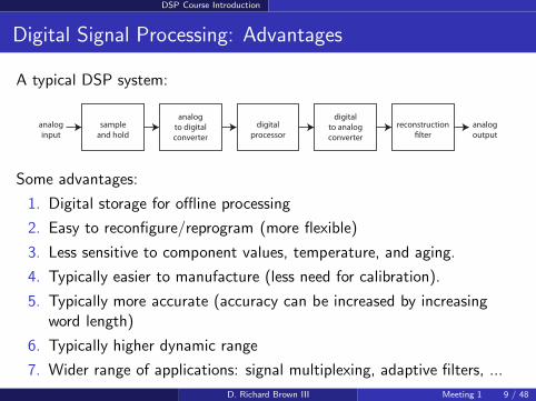
A typical DSP system:
analog
input
sample
and hold
analog
to digital
converter
digital
processor
digital
to analog
converter
reconstruction
lter
analog
output
Some advantages:
1. Digital storage for offline processing
2. Easy to reconfigure/reprogram (more flexible)
3. Less sensitive to component values, temperature, and aging.
4. Typically easier to manufacture (less need for calibration).
5. Typically more accurate (accuracy can be increased by increasingword length)
6. Typically higher dynamic range
7. Wider range of applications: signal multiplexing, adaptive filters, ...
D. Richard Brown III Meeting 1 9 / 48
DSP Course Introduction
Digital Signal Processing: Disadvantages
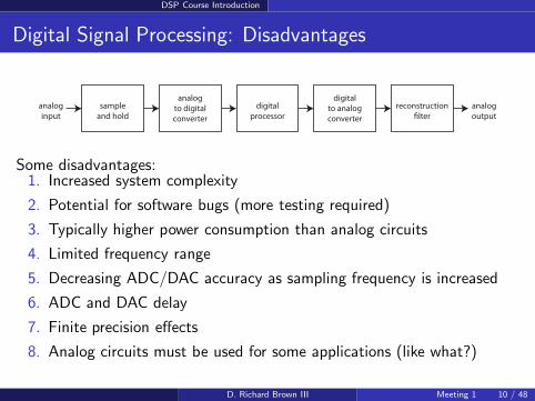
analog
input
sample
and hold
analog
to digital
converter
digital
processor
digital
to analog
converter
reconstruction
lter
analog
output
Some disadvantages:1. Increased system complexity
2. Potential for software bugs (more testing required)
3. Typically higher power consumption than analog circuits
4. Limited frequency range
5. Decreasing ADC/DAC accuracy as sampling frequency is increased
6. ADC and DAC delay
7. Finite precision effects
8. Analog circuits must be used for some applications (like what?)
D. Richard Brown III Meeting 1 10 / 48
DSP Course Introduction
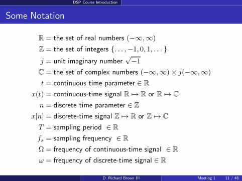
Some Notation
R = the set of real numbers (−∞,∞)
Z = the set of integers . . . ,−1, 0, 1, . . . j = unit imaginary number
√−1
C = the set of complex numbers (−∞,∞)× j(−∞,∞)
t = continuous time parameter ∈ R
x(t) = continuous-time signal R 7→ R or R 7→ C
n = discrete time parameter ∈ Z
x[n] = discrete-time signal Z 7→ R or Z 7→ C
T = sampling period ∈ R
fs = sampling frequency ∈ R
Ω = frequency of continuous-time signal ∈ R
ω = frequency of discrete-time signal ∈ R
D. Richard Brown III Meeting 1 11 / 48
DSP Course Introduction
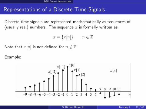
Representations of a Discrete-Time Signals
Discrete-time signals are represented mathematically as sequences of(usually real) numbers. The sequence x is formally written as
x = x[n] n ∈ Z
Note that x[n] is not defined for n /∈ Z.
Example:
D. Richard Brown III Meeting 1 12 / 48
DSP Course Introduction
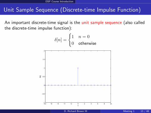
Unit Sample Sequence (Discrete-time Impulse Function)
An important discrete-time signal is the unit sample sequence (also calledthe discrete-time impulse function):
δ[n] =
1 n = 0
0 otherwise
−10 −8 −6 −4 −2 0 2 4 6 8 10−1
−0.5
0
0.5
1
1.5
2
n
δ[n]
D. Richard Brown III Meeting 1 13 / 48
DSP Course Introduction
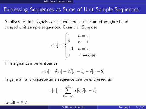
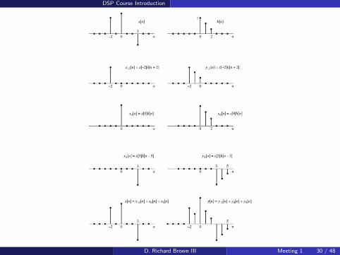
Expressing Sequences as Sums of Unit Sample Sequences
All discrete time signals can be written as the sum of weighted anddelayed unit sample sequences. Example: Suppose
x[n] =
1 n = 0
2 n = 1
−1 n = 2
0 otherwise
This signal can be written as
x[n] = δ[n] + 2δ[n − 1]− δ[n − 2]
In general, any discrete-time sequence can be expressed as
x[n] =∞∑
k=−∞
x[k]δ[n − k]
for all n ∈ Z.D. Richard Brown III Meeting 1 14 / 48
DSP Course Introduction
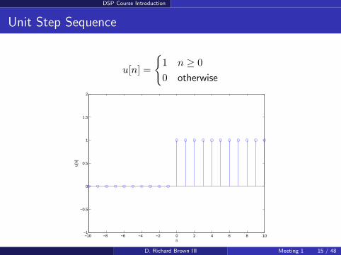
Unit Step Sequence
u[n] =
1 n ≥ 0
0 otherwise
−10 −8 −6 −4 −2 0 2 4 6 8 10−1
−0.5
0
0.5
1
1.5
2
n
u[n]
D. Richard Brown III Meeting 1 15 / 48
DSP Course Introduction
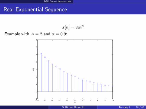
Real Exponential Sequence
x[n] = Aαn
Example with A = 2 and α = 0.9:
−10 −8 −6 −4 −2 0 2 4 6 8 10−1
0
1
2
3
4
5
6
7
n
x[n]
D. Richard Brown III Meeting 1 16 / 48
DSP Course Introduction
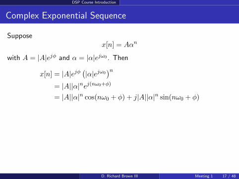
Complex Exponential Sequence
Supposex[n] = Aαn
with A = |A|ejφ and α = |α|ejω0 . Then
x[n] = |A|ejφ(|α|ejω0
)n
= |A||α|nej(nω0+φ)
= |A||α|n cos(nω0 + φ) + j|A||α|n sin(nω0 + φ)
D. Richard Brown III Meeting 1 17 / 48
DSP Course Introduction
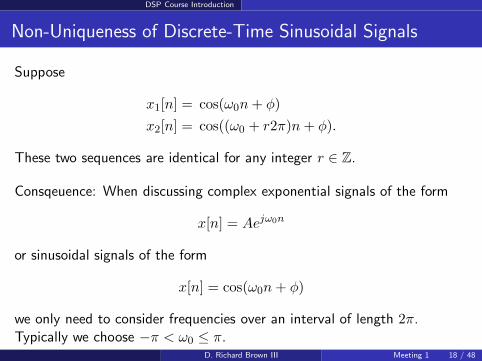
Non-Uniqueness of Discrete-Time Sinusoidal Signals
Suppose
x1[n] = cos(ω0n+ φ)
x2[n] = cos((ω0 + r2π)n+ φ).
These two sequences are identical for any integer r ∈ Z.
Consqeuence: When discussing complex exponential signals of the form
x[n] = Aejω0n
or sinusoidal signals of the form
x[n] = cos(ω0n+ φ)
we only need to consider frequencies over an interval of length 2π.Typically we choose −π < ω0 ≤ π.
D. Richard Brown III Meeting 1 18 / 48
DSP Course Introduction
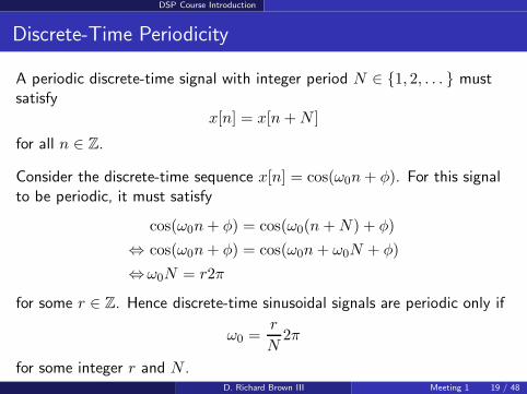
Discrete-Time Periodicity
A periodic discrete-time signal with integer period N ∈ 1, 2, . . . mustsatisfy
x[n] = x[n+N ]
for all n ∈ Z.
Consider the discrete-time sequence x[n] = cos(ω0n+ φ). For this signalto be periodic, it must satisfy
cos(ω0n+ φ) = cos(ω0(n+N) + φ)
⇔ cos(ω0n+ φ) = cos(ω0n+ ω0N + φ)
⇔ω0N = r2π
for some r ∈ Z. Hence discrete-time sinusoidal signals are periodic only if
ω0 =r
N2π
for some integer r and N .D. Richard Brown III Meeting 1 19 / 48
DSP Course Introduction
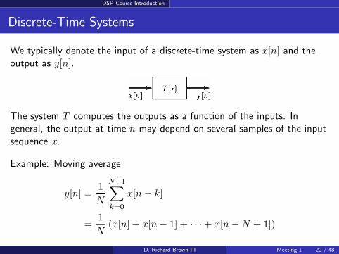
Discrete-Time Systems
We typically denote the input of a discrete-time system as x[n] and theoutput as y[n].
The system T computes the outputs as a function of the inputs. Ingeneral, the output at time n may depend on several samples of the inputsequence x.
Example: Moving average
y[n] =1
N
N−1∑
k=0
x[n− k]
=1
N(x[n] + x[n− 1] + · · ·+ x[n−N + 1])
D. Richard Brown III Meeting 1 20 / 48
DSP Course Introduction
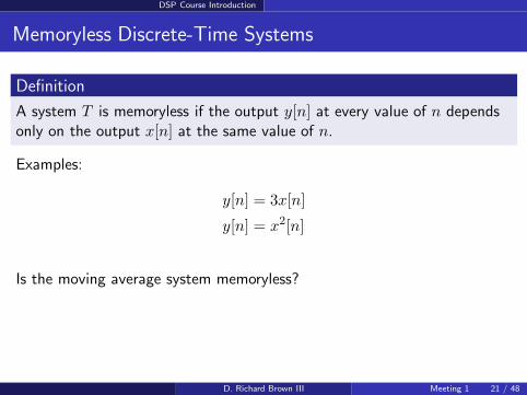
Memoryless Discrete-Time Systems
Definition
A system T is memoryless if the output y[n] at every value of n dependsonly on the output x[n] at the same value of n.
Examples:
y[n] = 3x[n]
y[n] = x2[n]
Is the moving average system memoryless?
D. Richard Brown III Meeting 1 21 / 48
DSP Course Introduction
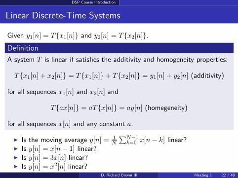
Linear Discrete-Time Systems
Given y1[n] = Tx1[n] and y2[n] = Tx2[n].Definition
A system T is linear if satisfies the additivity and homogeneity properties:
Tx1[n] + x2[n] = Tx1[n]+ Tx2[n] = y1[n] + y2[n] (additivity)
for all sequences x1[n] and x2[n] and
Tax[n] = aTx[n] = ay[n] (homegeneity)
for all sequences x[n] and any constant a.
Is the moving average y[n] = 1N
∑N−1k=0 x[n− k] linear?
Is y[n] = x[n− 1] linear? Is y[n] = 3x[n] linear? Is y[n] = x2[n] linear?
D. Richard Brown III Meeting 1 22 / 48
DSP Course Introduction
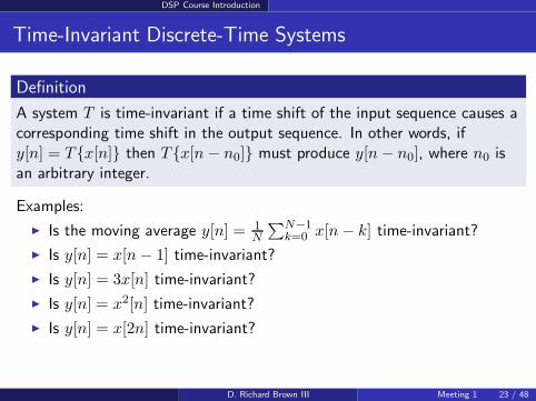
Time-Invariant Discrete-Time Systems
Definition
A system T is time-invariant if a time shift of the input sequence causes acorresponding time shift in the output sequence. In other words, ify[n] = Tx[n] then Tx[n − n0] must produce y[n− n0], where n0 isan arbitrary integer.
Examples:
Is the moving average y[n] = 1N
∑N−1k=0 x[n− k] time-invariant?
Is y[n] = x[n− 1] time-invariant?
Is y[n] = 3x[n] time-invariant?
Is y[n] = x2[n] time-invariant?
Is y[n] = x[2n] time-invariant?
D. Richard Brown III Meeting 1 23 / 48
DSP Course Introduction
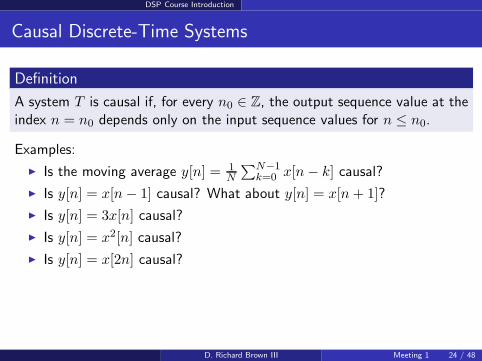
Causal Discrete-Time Systems
Definition
A system T is causal if, for every n0 ∈ Z, the output sequence value at theindex n = n0 depends only on the input sequence values for n ≤ n0.
Examples:
Is the moving average y[n] = 1N
∑N−1k=0 x[n− k] causal?
Is y[n] = x[n− 1] causal? What about y[n] = x[n+ 1]?
Is y[n] = 3x[n] causal?
Is y[n] = x2[n] causal?
Is y[n] = x[2n] causal?
D. Richard Brown III Meeting 1 24 / 48
DSP Course Introduction
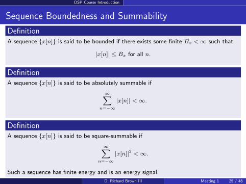
Sequence Boundedness and Summability
DefinitionA sequence x[n] is said to be bounded if there exists some finite Bx < ∞ such that
|x[n]| ≤ Bx for all n.
DefinitionA sequence x[n] is said to be absolutely summable if
∞∑
n=−∞
|x[n]| < ∞.
DefinitionA sequence x[n] is said to be square-summable if
∞∑
n=−∞
|x[n]|2 < ∞.
Such a sequence has finite energy and is an energy signal.
D. Richard Brown III Meeting 1 25 / 48
DSP Course Introduction
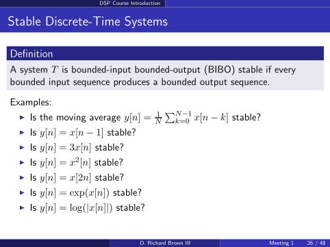
Stable Discrete-Time Systems
Definition
A system T is bounded-input bounded-output (BIBO) stable if everybounded input sequence produces a bounded output sequence.
Examples:
Is the moving average y[n] = 1N
∑N−1k=0 x[n− k] stable?
Is y[n] = x[n− 1] stable?
Is y[n] = 3x[n] stable?
Is y[n] = x2[n] stable?
Is y[n] = x[2n] stable?
Is y[n] = exp(x[n]) stable?
Is y[n] = log(|x[n]|) stable?
D. Richard Brown III Meeting 1 26 / 48
DSP Course Introduction
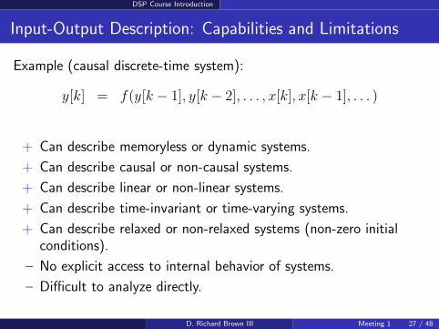
Input-Output Description: Capabilities and Limitations
Example (causal discrete-time system):
y[k] = f(y[k − 1], y[k − 2], . . . , x[k], x[k − 1], . . . )
+ Can describe memoryless or dynamic systems.
+ Can describe causal or non-causal systems.
+ Can describe linear or non-linear systems.
+ Can describe time-invariant or time-varying systems.
+ Can describe relaxed or non-relaxed systems (non-zero initialconditions).
– No explicit access to internal behavior of systems.
– Difficult to analyze directly.
D. Richard Brown III Meeting 1 27 / 48
DSP Course Introduction
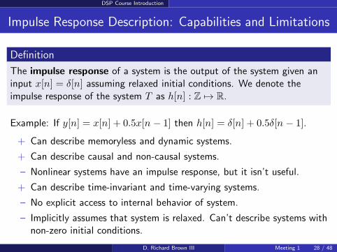
Impulse Response Description: Capabilities and Limitations
Definition
The impulse response of a system is the output of the system given aninput x[n] = δ[n] assuming relaxed initial conditions. We denote theimpulse response of the system T as h[n] : Z 7→ R.
Example: If y[n] = x[n] + 0.5x[n − 1] then h[n] = δ[n] + 0.5δ[n − 1].
+ Can describe memoryless and dynamic systems.
+ Can describe causal and non-causal systems.
– Nonlinear systems have an impulse response, but it isn’t useful.
+ Can describe time-invariant and time-varying systems.
– No explicit access to internal behavior of system.
– Implicitly assumes that system is relaxed. Can’t describe systems withnon-zero initial conditions.
D. Richard Brown III Meeting 1 28 / 48
DSP Course Introduction
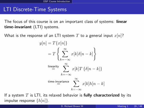
LTI Discrete-Time Systems
The focus of this course is on an important class of systems: lineartime-invariant (LTI) systems.
What is the response of an LTI system T to a general input x[n]?
y[n] = Tx[n]
= T
∞∑
k=−∞
x[k]δ[n − k]
linearity=
∞∑
k=−∞
x[k]T δ[n − k]
time-invariance=
∞∑
k=−∞
x[k]h[n − k]
If a system T is LTI, its relaxed behavior is fully characterized by itsimpulse response h[n].
D. Richard Brown III Meeting 1 29 / 48
DSP Course Introduction
D. Richard Brown III Meeting 1 30 / 48
DSP Course Introduction
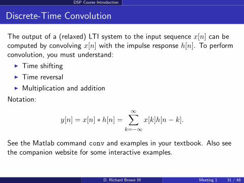
Discrete-Time Convolution
The output of a (relaxed) LTI system to the input sequence x[n] can becomputed by convolving x[n] with the impulse response h[n]. To performconvolution, you must understand:
Time shifting
Time reversal
Multiplication and addition
Notation:
y[n] = x[n] ∗ h[n] =∞∑
k=−∞
x[k]h[n − k].
See the Matlab command conv and examples in your textbook. Also seethe companion website for some interactive examples.
D. Richard Brown III Meeting 1 31 / 48
DSP Course Introduction
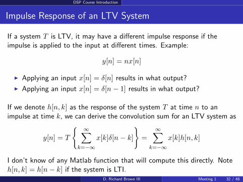
Impulse Response of an LTV System
If a system T is LTV, it may have a different impulse response if theimpulse is applied to the input at different times. Example:
y[n] = nx[n]
Applying an input x[n] = δ[n] results in what output?
Applying an input x[n] = δ[n − 1] results in what output?
If we denote h[n, k] as the response of the system T at time n to animpulse at time k, we can derive the convolution sum for an LTV system as
y[n] = T
∞∑
k=−∞
x[k]δ[n − k]
=∞∑
k=−∞
x[k]h[n, k]
I don’t know of any Matlab function that will compute this directly. Noteh[n, k] = h[n − k] if the system is LTI.
D. Richard Brown III Meeting 1 32 / 48
DSP Course Introduction
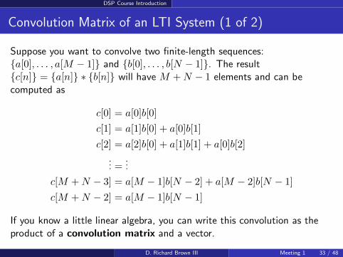
Convolution Matrix of an LTI System (1 of 2)
Suppose you want to convolve two finite-length sequences:a[0], . . . , a[M − 1] and b[0], . . . , b[N − 1]. The resultc[n] = a[n] ∗ b[n] will have M +N − 1 elements and can becomputed as
c[0] = a[0]b[0]
c[1] = a[1]b[0] + a[0]b[1]
c[2] = a[2]b[0] + a[1]b[1] + a[0]b[2]
... =...
c[M +N − 3] = a[M − 1]b[N − 2] + a[M − 2]b[N − 1]
c[M +N − 2] = a[M − 1]b[N − 1]
If you know a little linear algebra, you can write this convolution as theproduct of a convolution matrix and a vector.
D. Richard Brown III Meeting 1 33 / 48
DSP Course Introduction
Convolution Matrix of an LTI System (2 of 2)
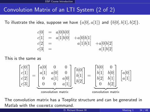
To illustrate the idea, suppose we have a[0], a[1] and b[0], b[1], b[2].
c[0] = a[0]b[0]c[1] = a[1]b[0] +a[0]b[1]c[2] = a[1]b[1] +a[0]b[2]c[3] = a[1]b[2]
This is the same as
c[0]c[1]c[2]c[3]
=
a[0] 0 0a[1] a[0] 00 a[1] a[0]0 0 a[1]
︸ ︷︷ ︸
convolution matrix
b[0]b[1]b[2]
=
b[0] 0b[1] b[0]b[2] b[1]0 b[2]
︸ ︷︷ ︸
convolution matrix
[a[0]a[1]
]
The convolution matrix has a Toeplitz structure and can be generated inMatlab with the convmtx command.
D. Richard Brown III Meeting 1 34 / 48
DSP Course Introduction
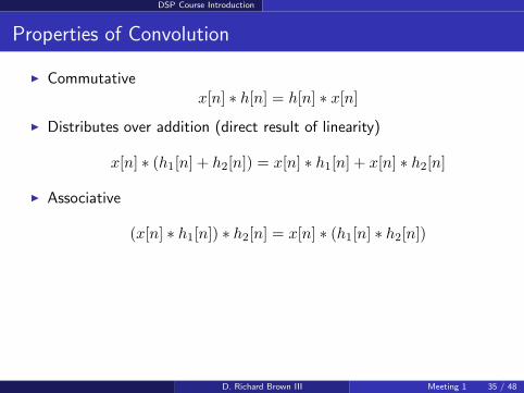
Properties of Convolution
Commutativex[n] ∗ h[n] = h[n] ∗ x[n]
Distributes over addition (direct result of linearity)
x[n] ∗ (h1[n] + h2[n]) = x[n] ∗ h1[n] + x[n] ∗ h2[n]
Associative
(x[n] ∗ h1[n]) ∗ h2[n] = x[n] ∗ (h1[n] ∗ h2[n])
D. Richard Brown III Meeting 1 35 / 48
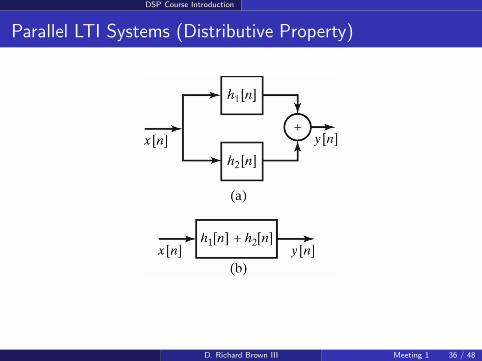
DSP Course Introduction
Parallel LTI Systems (Distributive Property)
D. Richard Brown III Meeting 1 36 / 48
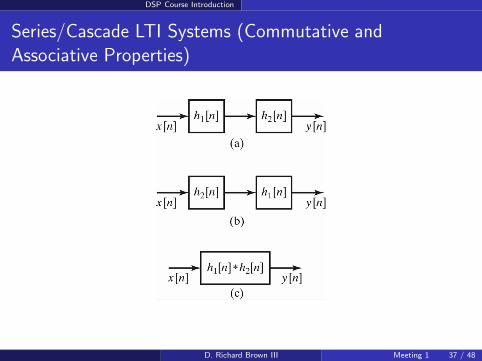
DSP Course Introduction
Series/Cascade LTI Systems (Commutative and
Associative Properties)
D. Richard Brown III Meeting 1 37 / 48
DSP Course Introduction
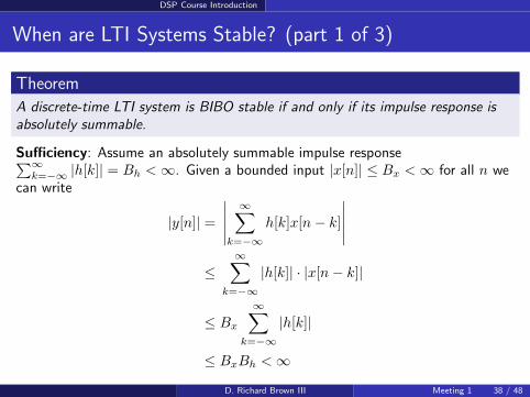
When are LTI Systems Stable? (part 1 of 3)
Theorem
A discrete-time LTI system is BIBO stable if and only if its impulse response is
absolutely summable.
Sufficiency: Assume an absolutely summable impulse response∑
∞
k=−∞|h[k]| = Bh < ∞. Given a bounded input |x[n]| ≤ Bx < ∞ for all n we
can write
|y[n]| =∣∣∣∣∣
∞∑
k=−∞
h[k]x[n− k]
∣∣∣∣∣
≤∞∑
k=−∞
|h[k]| · |x[n− k]|
≤ Bx
∞∑
k=−∞
|h[k]|
≤ BxBh < ∞
D. Richard Brown III Meeting 1 38 / 48
DSP Course Introduction
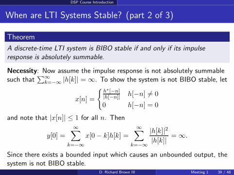
When are LTI Systems Stable? (part 2 of 3)
Theorem
A discrete-time LTI system is BIBO stable if and only if its impulse
response is absolutely summable.
Necessity: Now assume the impulse response is not absolutely summablesuch that
∑∞k=−∞ |h[k]| = ∞. To show the system is not BIBO stable, let
x[n] =
h∗[−n]|h[−n]| h[−n] 6= 0
0 h[−n] = 0
and note that |x[n]| ≤ 1 for all n. Then
y[0] =∞∑
k=−∞
x[0− k]h[k] =∞∑
k=−∞
|h[k]|2|h[k]| = ∞.
Since there exists a bounded input which causes an unbounded output, thesystem is not BIBO stable.
D. Richard Brown III Meeting 1 39 / 48
DSP Course Introduction
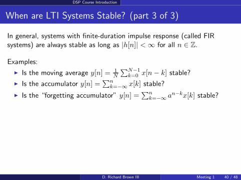
When are LTI Systems Stable? (part 3 of 3)
In general, systems with finite-duration impulse response (called FIRsystems) are always stable as long as |h[n]| < ∞ for all n ∈ Z.
Examples:
Is the moving average y[n] = 1N
∑N−1k=0 x[n− k] stable?
Is the accumulator y[n] =∑n
k=−∞ x[k] stable?
Is the “forgetting accumulator” y[n] =∑n
k=−∞ an−kx[k] stable?
D. Richard Brown III Meeting 1 40 / 48
DSP Course Introduction
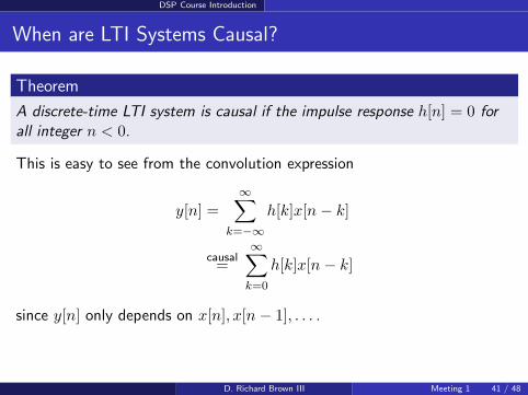
When are LTI Systems Causal?
Theorem
A discrete-time LTI system is causal if the impulse response h[n] = 0 for
all integer n < 0.
This is easy to see from the convolution expression
y[n] =
∞∑
k=−∞
h[k]x[n − k]
causal=
∞∑
k=0
h[k]x[n − k]
since y[n] only depends on x[n], x[n − 1], . . . .
D. Richard Brown III Meeting 1 41 / 48
DSP Course Introduction
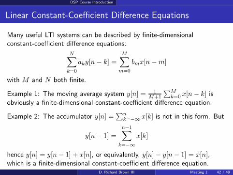
Linear Constant-Coefficient Difference Equations
Many useful LTI systems can be described by finite-dimensionalconstant-coefficient difference equations:
N∑
k=0
aky[n− k] =
M∑
m=0
bmx[n−m]
with M and N both finite.
Example 1: The moving average system y[n] = 1M+1
∑Mk=0 x[n− k] is
obviously a finite-dimensional constant-coefficient difference equation.
Example 2: The accumulator y[n] =∑n
k=−∞ x[k] is not in this form. But
y[n− 1] =
n−1∑
k=−∞
x[k]
hence y[n] = y[n− 1] + x[n], or equivalently, y[n]− y[n− 1] = x[n],which is a finite-dimensional constant-coefficient difference equation.
D. Richard Brown III Meeting 1 42 / 48
DSP Course Introduction
Linear Constant-Coefficient Difference Equations
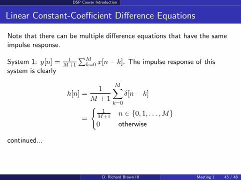
Note that there can be multiple difference equations that have the sameimpulse response.
System 1: y[n] = 1M+1
∑Mk=0 x[n− k]. The impulse response of this
system is clearly
h[n] =1
M + 1
M∑
k=0
δ[n − k]
=
1
M+1 n ∈ 0, 1, . . . ,M0 otherwise
continued...
D. Richard Brown III Meeting 1 43 / 48
DSP Course Introduction
Linear Constant-Coefficient Difference Equations
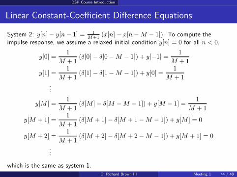
System 2: y[n]− y[n− 1] = 1
M+1(x[n]− x[n−M − 1]). To compute the
impulse response, we assume a relaxed initial condition y[n] = 0 for all n < 0.
y[0] =1
M + 1(δ[0]− δ[0−M − 1]) + y[−1] =
1
M + 1
y[1] =1
M + 1(δ[1]− δ[1−M − 1]) + y[0] =
1
M + 1...
y[M ] =1
M + 1(δ[M ]− δ[M −M − 1]) + y[M − 1] =
1
M + 1
y[M + 1] =1
M + 1(δ[M + 1]− δ[M + 1−M − 1]) + y[M ] = 0
y[M + 2] =1
M + 1(δ[M + 2]− δ[M + 2−M − 1]) + y[M + 1] = 0
...
which is the same as system 1.D. Richard Brown III Meeting 1 44 / 48
DSP Course Introduction
Solving LTI Systems Described by Difference Equations
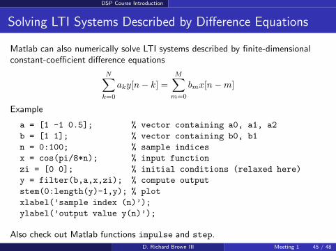
Matlab can also numerically solve LTI systems described by finite-dimensionalconstant-coefficient difference equations
N∑
k=0
aky[n− k] =
M∑
m=0
bmx[n−m]
Example
a = [1 -1 0.5]; % vector containing a0, a1, a2
b = [1 1]; % vector containing b0, b1
n = 0:100; % sample indices
x = cos(pi/8*n); % input function
zi = [0 0]; % initial conditions (relaxed here)
y = filter(b,a,x,zi); % compute output
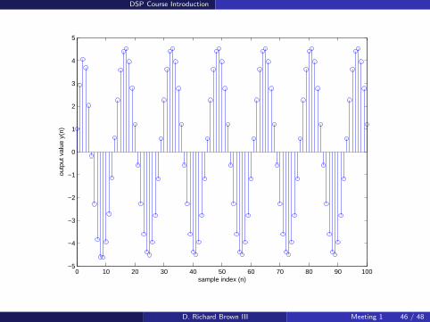
stem(0:length(y)-1,y); % plot
xlabel(’sample index (n)’);
ylabel(’output value y(n)’);
Also check out Matlab functions impulse and step.D. Richard Brown III Meeting 1 45 / 48
DSP Course Introduction
0 10 20 30 40 50 60 70 80 90 100−5
−4
−3
−2
−1
0
1
2
3
4
5
sample index (n)
outp
ut v
alue
y(n
)
D. Richard Brown III Meeting 1 46 / 48
DSP Course Introduction
Summary
1. Discrete-time signals
2. Discrete-time systems and qualitative properties (linearity,time-invariance, causality, stability)
3. DT-LTI systems
4. Impulse response and convolution
5. Linear constant-coefficient difference equations
D. Richard Brown III Meeting 1 47 / 48
DSP Course Introduction
What’s Next?
This is the only “lecture” in ECE503. The remaining class meetings will bestructured as
First half: Discussion/examples related to reading assignment,screencasts, suggested problems.
Second half: 60-minute quiz.
Next week’s meeting will be focused on topics in Chapter 2 of yourtextbook.
Any questions/discussion during the week should be posted to Piazza.Students are encouraged to collaborate on everything except the quizzes.
D. Richard Brown III Meeting 1 48 / 48