Embed Size (px)
Citation preview
TelecommunicationsCommunications Technologies
Digital Modulation(PCM/DPCM/Delta)
Courseware Sample39863-F0
A


TELECOMMUNICATIONSCOMMUNICATIONS TECHNOLOGIES
DIGITAL MODULATION (PCM/DPCM/DELTA)
Courseware Sample
bythe Staff
ofLab-Volt Ltd.
Copyright © 2009 Lab-Volt Ltd.
All rights reserved. No part of this publication may be reproduced,in any form or by any means, without the prior written permissionof Lab-Volt Ltd.
Printed in CanadaJanuary 2010
III
Table of ContentsForeword
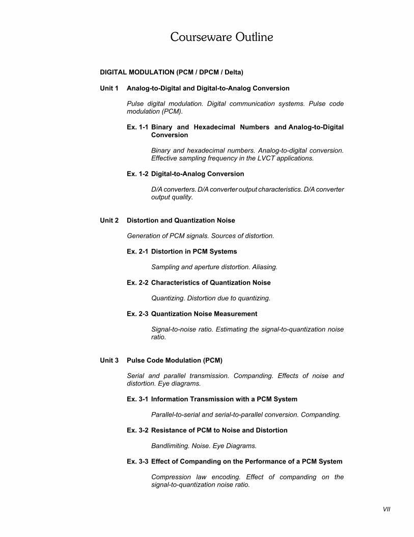
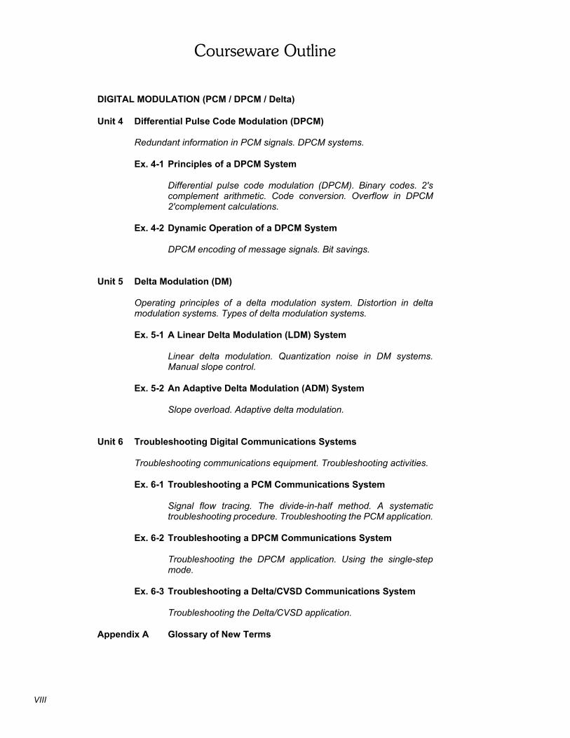
Courseware Outline
Digital Modulation (PCM / DPCM / Delta)
Sample Exercise Extracted from Digital Modulation (PCM / DPCM / Delta)
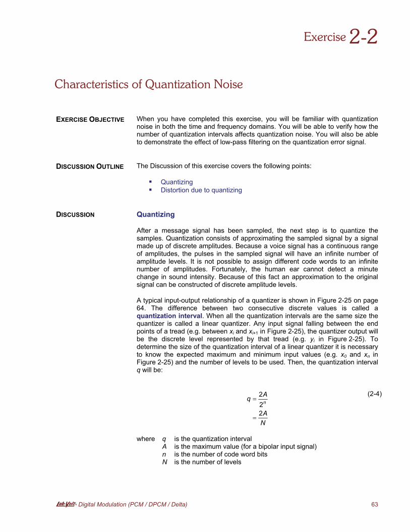
Exercise 2-2 Characteristics of Quantization Noise
Other Sample Extracted from Digital Modulation (PCM / DPCM / Delta)
Unit Test 2 Distortion and Quantization Noise
Instructor Guide Sample Exercise Extracted from Digital Modulation (PCM /DPCM / Delta)
Exercise 2-2 Characteristics of Quantization Noise
Bibliography

IV
V
Foreword
Digital communication offers so many advantages over analog communication thatthe majority of today's communications systems are digital.
Unlike analog communication systems, digital systems do not require accuraterecovery of the transmitted waveform at the receiver end. Instead, the receiverperiodically detects which waveform is being transmitted, among a limited numberof possible waveforms, and maps the detected waveform back to the data itrepresents. This allows extremely low error rates, even when the signal has beencorrupted by noise.
The digital circuits are often implemented using application specific integratedcircuits (ASIC) and field-programmable gate arrays (FPGA). Although this"system-on-a-chip" approach is very effective for commercial and militaryapplications, the resulting systems do not allow access to internal signals and dataand are therefore poorly suited for educational use. It is for this reason that Lab-Voltdesigned the Communications Technologies Training System.
The Lab-Volt Communications Technologies Training System, Model 8087, is astate-of-the-art communications training system. Specially designed for hands-ontraining, it facilitates the study of many different types of digitalmodulation/demodulation technologies such as PAM, PWM, PPM, PCM, DeltaModulation, ASK, FSK, and BPSK as well as spectrally efficient technologies suchas QPSK, QAM, and ADSL. The system is designed to reflect the standardscommonly used in modern communications systems.
Unlike conventional, hardware-based training systems that use a variety of physicalmodules to implement different technologies and instruments, the CommunicationsTechnologies Training System is based on a Reconfigurable Training Module (RTM)and the Lab-Volt Communications Technologies (LVCT) software, providingtremendous flexibility at a reduced cost.
Each of the communications technologies to be studied is provided as an applicationthat can be selected from a menu. Once loaded into the LVCT software, the selectedapplication configures the RTM to implement the communications technology, andprovides a specially designed user interface for the student.
The LVCT software provides settings for full user control over the operatingparameters of each communications technology application. Functional blockdiagrams for the circuits involved are shown on screen. The digital or analog signalsat various points in the circuits can be viewed and analyzed using the virtualinstruments included in the software. In addition, some of these signals are madeavailable at physical connectors on the RTM and can be displayed and measuredusing conventional instruments.
The courseware for the Communications Technologies Training System consists ofa series of student manuals covering the different technologies as well as instructorguides that provide the answers to procedure step questions and to reviewquestions. The Communications Technologies Training System and theaccompanying courseware provide a complete study program for these keyinformation-age technologies.

VI
DIGITAL MODULATION (PCM / DPCM / Delta)
Courseware Outline
VII
Unit 1 Analog-to-Digital and Digital-to-Analog Conversion
Pulse digital modulation. Digital communication systems. Pulse codemodulation (PCM).
Ex. 1-1 Binary and Hexadecimal Numbers and Analog-to-DigitalConversion
Binary and hexadecimal numbers. Analog-to-digital conversion.Effective sampling frequency in the LVCT applications.
Ex. 1-2 Digital-to-Analog Conversion
D/A converters. D/A converter output characteristics. D/A converteroutput quality.
Unit 2 Distortion and Quantization Noise
Generation of PCM signals. Sources of distortion.
Ex. 2-1 Distortion in PCM Systems
Sampling and aperture distortion. Aliasing.
Ex. 2-2 Characteristics of Quantization Noise
Quantizing. Distortion due to quantizing.
Ex. 2-3 Quantization Noise Measurement
Signal-to-noise ratio. Estimating the signal-to-quantization noiseratio.
Unit 3 Pulse Code Modulation (PCM)
Serial and parallel transmission. Companding. Effects of noise anddistortion. Eye diagrams.
Ex. 3-1 Information Transmission with a PCM System
Parallel-to-serial and serial-to-parallel conversion. Companding.
Ex. 3-2 Resistance of PCM to Noise and Distortion
Bandlimiting. Noise. Eye Diagrams.
Ex. 3-3 Effect of Companding on the Performance of a PCM System
Compression law encoding. Effect of companding on thesignal-to-quantization noise ratio.
DIGITAL MODULATION (PCM / DPCM / Delta)
Courseware Outline
VIII
Unit 4 Differential Pulse Code Modulation (DPCM)
Redundant information in PCM signals. DPCM systems.
Ex. 4-1 Principles of a DPCM System
Differential pulse code modulation (DPCM). Binary codes. 2'scomplement arithmetic. Code conversion. Overflow in DPCM2'complement calculations.
Ex. 4-2 Dynamic Operation of a DPCM System
DPCM encoding of message signals. Bit savings.
Unit 5 Delta Modulation (DM)
Operating principles of a delta modulation system. Distortion in deltamodulation systems. Types of delta modulation systems.
Ex. 5-1 A Linear Delta Modulation (LDM) System
Linear delta modulation. Quantization noise in DM systems.Manual slope control.
Ex. 5-2 An Adaptive Delta Modulation (ADM) System
Slope overload. Adaptive delta modulation.
Unit 6 Troubleshooting Digital Communications Systems
Troubleshooting communications equipment. Troubleshooting activities.
Ex. 6-1 Troubleshooting a PCM Communications System
Signal flow tracing. The divide-in-half method. A systematictroubleshooting procedure. Troubleshooting the PCM application.
Ex. 6-2 Troubleshooting a DPCM Communications System
Troubleshooting the DPCM application. Using the single-stepmode.
Ex. 6-3 Troubleshooting a Delta/CVSD Communications System
Troubleshooting the Delta/CVSD application.
Appendix A Glossary of New Terms
Sample Exercise
Extracted from
Digital Modulation
(PCM / DPCM / Delta)

Digital Modulation (PCM / DPCM / Delta) 63
When you have completed this exercise, you will be familiar with quantization noise in both the time and frequency domains. You will be able to verify how the number of quantization intervals affects quantization noise. You will also be able to demonstrate the effect of low-pass filtering on the quantization error signal.
The Discussion of this exercise covers the following points:
� Quantizing�� Distortion due to quantizing�
Quantizing
After a message signal has been sampled, the next step is to quantize the samples. Quantization consists of approximating the sampled signal by a signal made up of discrete amplitudes. Because a voice signal has a continuous range of amplitudes, the pulses in the sampled signal will have an infinite number of amplitude levels. It is not possible to assign different code words to an infinite number of amplitudes. Fortunately, the human ear cannot detect a minute change in sound intensity. Because of this fact an approximation to the original signal can be constructed of discrete amplitude levels.
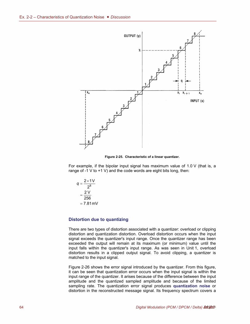
A typical input-output relationship of a quantizer is shown in Figure 2-25 on page 64. The difference between two consecutive discrete values is called a quantization interval. When all the quantization intervals are the same size the quantizer is called a linear quantizer. Any input signal falling between the end points of a tread (e.g. between xi and xi+1 in Figure 2-25), the quantizer output will be the discrete level represented by that tread (e.g. yi in Figure 2-25). To determine the size of the quantization interval of a linear quantizer it is necessary to know the expected maximum and minimum input values (e.g. x0 and xn in Figure 2-25) and the number of levels to be used. Then, the quantization interval q will be:
NA
Aq n
222
�
�
(2-4)
where q is the quantization interval A is the maximum value (for a bipolar input signal) n is the number of code word bits N is the number of levels
Characteristics of Quantization Noise
Exercise 2-2
EXERCISE OBJECTIVE
DISCUSSION OUTLINE
DISCUSSION
Ex. 2-2 – Characteristics of Quantization Noise � Discussion
64 Digital Modulation (PCM / DPCM / Delta)
Figure 2-25. Characteristic of a linear quantizer.
For example, if the bipolar input signal has maximum value of 1.0 V (that is, a range of -1 V to +1 V) and the code words are eight bits long, then:
mV81.7256
V22
V128
�
�
��q
Distortion due to quantizing
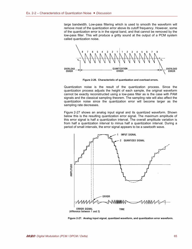
There are two types of distortion associated with a quantizer: overload or clipping distortion and quantization distortion. Overload distortion occurs when the input signal exceeds the quantizer's input range. Once the quantizer range has been exceeded the output will remain at its maximum (or minimum) value until the input falls within the quantizer's input range. As was seen in Unit 1, overload distortion results in a clipped output signal. To avoid clipping, a quantizer is matched to the input signal.
Figure 2-26 shows the error signal introduced by the quantizer. From this figure, it can be seen that quantization error occurs when the input signal is within the input range of the quantizer. It arises because of the difference between the input amplitude and the quantized sampled amplitude and because of the limited sampling rate. The quantization error signal produces quantization noise or distortion in the reconstructed message signal. Its frequency spectrum covers a
Ex. 2-2 – Characteristics of Quantization Noise � Discussion
Digital Modulation (PCM / DPCM / Delta) 65
large bandwidth. Low-pass filtering which is used to smooth the waveform will remove most of the quantization error above its cutoff frequency. However, some of the quantization error is in the signal band, and that cannot be removed by the low-pass filter. This will produce a gritty sound at the output of a PCM system called quantization noise.
Figure 2-26.�Characteristic of quantization and overload errors.
Quantization noise is the result of the quantization process. Since the quantization process adjusts the height of each sample, the original waveform cannot be exactly reconstructed using a low-pass filter as is the case with PAM signals and the classical sampling theorem. The sampling rate will also affect the quantization noise since the quantization error will become larger as the sampling rate decreases.
Figure 2-27 shows an analog input signal and its quantized waveform. Shown below this is the resulting quantization error signal. The maximum amplitude of this error signal is half a quantization interval. The overall amplitude variation is from half a quantization interval to minus half a quantization interval. During a period of small intervals, the error signal appears to be a sawtooth wave.
Figure 2-27.�Analog input signal, quantized waveform, and quantization error waveform.
Ex. 2-2 – Characteristics of Quantization Noise � Procedure Outline
66 Digital Modulation (PCM / DPCM / Delta)
The Procedure is divided into the following sections:
� Set up and connections�� Effect of sampling frequency on quantization noise�� Effect of resolution on quantization noise�� Effect of low-pass filtering the PCM Decoder output signal�
Set up and connections
1. Turn on the RTM Power Supply and the RTM and make sure the RTM power LED is lit.
2. Start the LVCT software. In the Application Selection box, choose PCM and click OK. This begins a new session with all settings set to their default values and with all faults deactivated.
b If the software is already running, choose Exit in the File menu and restart LVCT to begin a new session with all faults deactivated.
3. Make the Default external connections shown on the System Diagram tab of the software. For details of connections to the Reconfigurable Training Module, refer to the RTM Connections tab of the software.
b Click the Default button to show the required external connections.
4. As an option, use a conventional oscilloscope during this exercise to observe any of the outputs on the RTM (refer to the RTM Connections tab of the software for the available outputs). Use BNC T-connectors where necessary.
Effect of sampling frequency on quantization noise
5. Make the following settings:
Generator Settings
� Function Generator A Function ................................................... Sine Output level ............................................. 1.5 V Frequency ................................................ 1000 Hz
PCM Settings
� General Sampling Frequency ............................... 142 045 Hz
� Pre-Filtering Pre-Filtering ............................................. Off
� PCM Encoder Data source ............................................. A/D Compression Law .................................... Dir Bit Interruptor ........................................... 1111 1111
PROCEDURE OUTLINE
PROCEDURE
File � Restore Default Settings returns all settings to their default values, but does not deactivate activated faults.
Double-click to select SWapp
Select SWconnection
Ex. 2-2 – Characteristics of Quantization Noise � Procedure
Digital Modulation (PCM / DPCM / Delta) 67
� PCM Decoder Input Code ............................................... Offset Output Gain ............................................. 1
� Post-Filtering Notch 1 .................................................... Off Notch 1 Center Frequency ...................... 1000 Hz Low-Pass Cutoff Frequency .................... 3400 Hz Low-Pass Order ...................................... 4th Low-Pass Filter Coupling ........................ AC Notch 2 .................................................... Off
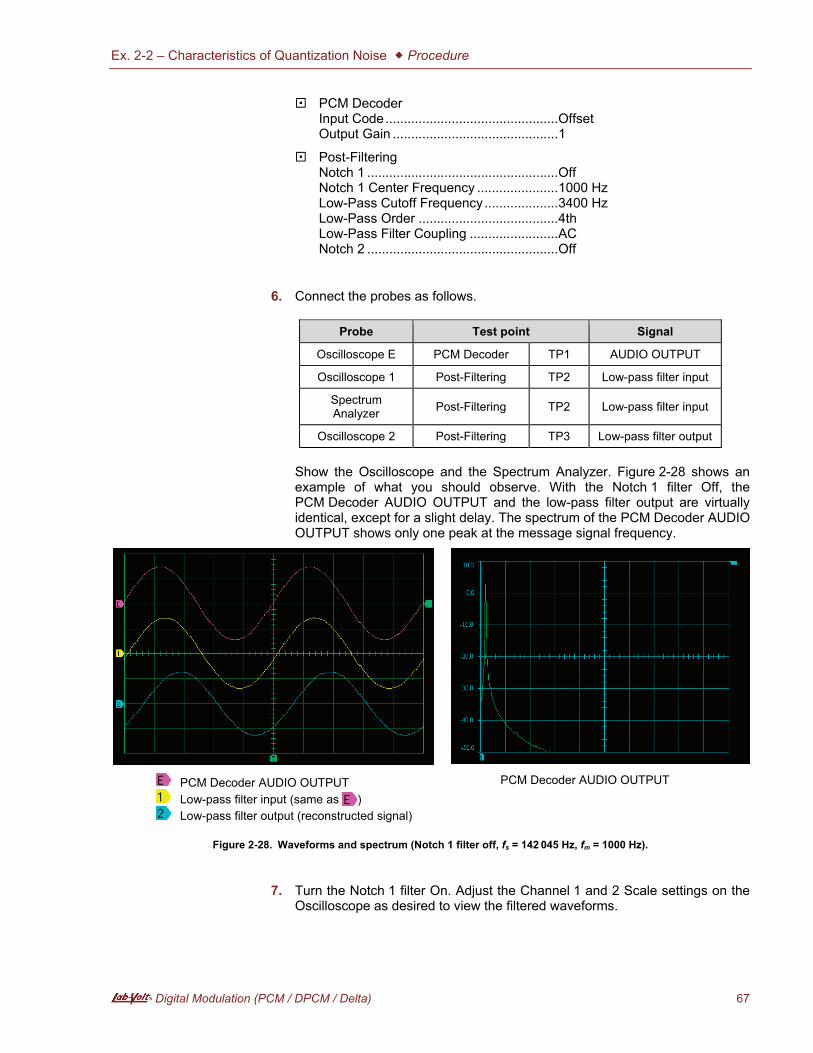
6. Connect the probes as follows.
Probe Test point Signal
Oscilloscope E PCM Decoder TP1 AUDIO OUTPUT
Oscilloscope 1 Post-Filtering TP2 Low-pass filter input
Spectrum Analyzer Post-Filtering TP2 Low-pass filter input
Oscilloscope 2 Post-Filtering TP3 Low-pass filter output
Show the Oscilloscope and the Spectrum Analyzer. Figure 2-28 shows an example of what you should observe. With the Notch 1 filter Off, the PCM Decoder AUDIO OUTPUT and the low-pass filter output are virtually identical, except for a slight delay. The spectrum of the PCM Decoder AUDIO OUTPUT shows only one peak at the message signal frequency.
PCM Decoder AUDIO OUTPUT Low-pass filter input (same as ) Low-pass filter output (reconstructed signal)
PCM Decoder AUDIO OUTPUT
Figure 2-28.�Waveforms and spectrum (Notch 1 filter off, fs = 142 045 Hz, fm = 1000 Hz).
7. Turn the Notch 1 filter On. Adjust the Channel 1 and 2 Scale settings on the Oscilloscope as desired to view the filtered waveforms.
Ex. 2-2 – Characteristics of Quantization Noise � Procedure
68 Digital Modulation (PCM / DPCM / Delta)
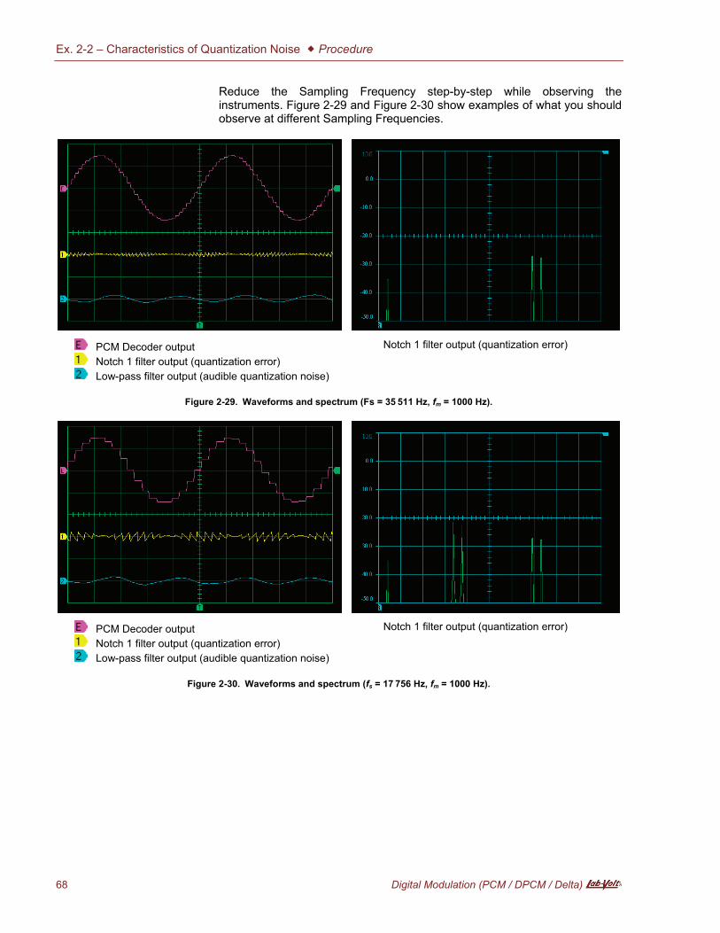
Reduce the Sampling Frequency step-by-step while observing the instruments. Figure 2-29 and Figure 2-30 show examples of what you should observe at different Sampling Frequencies.
PCM Decoder output Notch 1 filter output (quantization error) Low-pass filter output (audible quantization noise)
Notch 1 filter output (quantization error)
Figure 2-29.�Waveforms and spectrum (Fs = 35 511 Hz, fm = 1000 Hz).
PCM Decoder output Notch 1 filter output (quantization error) Low-pass filter output (audible quantization noise)
Notch 1 filter output (quantization error)
Figure 2-30.�Waveforms and spectrum (fs = 17 756 Hz, fm = 1000 Hz).
Ex. 2-2 – Characteristics of Quantization Noise � Procedure
Digital Modulation (PCM / DPCM / Delta) 69
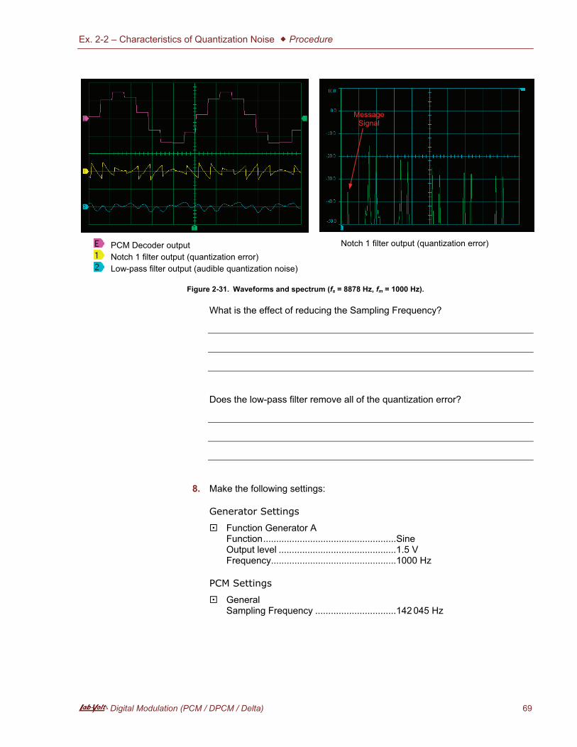
PCM Decoder output Notch 1 filter output (quantization error) Low-pass filter output (audible quantization noise)
Notch 1 filter output (quantization error)
Figure 2-31.�Waveforms and spectrum (fs = 8878 Hz, fm = 1000 Hz).
What is the effect of reducing the Sampling Frequency?
Does the low-pass filter remove all of the quantization error?
8. Make the following settings:
Generator Settings
� Function Generator A Function ................................................... Sine Output level ............................................. 1.5 V Frequency ................................................ 1000 Hz
PCM Settings
� General Sampling Frequency ............................... 142 045 Hz
Message Signal
Ex. 2-2 – Characteristics of Quantization Noise � Procedure
70 Digital Modulation (PCM / DPCM / Delta)
� Post-Filtering Notch 1 .................................................... Off Low-Pass Cutoff Frequency .................... 10 000 Hz Low-Pass Order....................................... 4th Low-Pass Filter Coupling ........................ AC Notch 2 .................................................... Off
Using the supplied adapter(s), connect the headphones to the Post-Filtering OUTPUT (refer to the RTM Connections tab of the software).
Gradually reduce the Sampling Frequency as you observe the spectrum and listen to the sound of the reconstructed signal.
What is the audible effect of reducing the Sampling Frequency on the reconstructed signal?
With a low Sampling Frequency setting, vary the Low-Pass Cutoff Frequency as you listen to the sound of the reconstructed signal. Is reducing the cutoff frequency of the low-pass filter an effective way to compensate for a low Sampling Frequency?
Effect of resolution on quantization noise
9. The probes should be connected as follows:
Probe Test point Signal
Oscilloscope E PCM Decoder TP1 AUDIO OUTPUT
Oscilloscope 1 Post-Filtering TP2 Notch 1 filter output
Spectrum Analyzer Post-Filtering TP2 Notch 1 filter output
Oscilloscope 2 Post-Filtering TP3 Low-pass filter output
Make the following settings:
Generator Settings
� Function Generator A Function ................................................... Sine Output level ............................................. 1.5 V Frequency ................................................ 1000 Hz
Ex. 2-2 – Characteristics of Quantization Noise � Procedure
Digital Modulation (PCM / DPCM / Delta) 71
PCM Settings
� General Sampling Frequency ............................... 35 511 Hz
� Pre-Filtering Pre-Filtering ............................................. Off
� PCM Encoder Data source ............................................. A/D Compression Law .................................... Dir Bit Interruptor ........................................... 1111 1111
� PCM Decoder Input Code ............................................... Offset Output Gain ............................................. 1
� Post-Filtering Notch 1 .................................................... On Notch 1 Center Frequency ...................... 1000 Hz Low-Pass Cutoff Frequency .................... 10 000 Hz Low-Pass Order ...................................... 4th Low-Pass Filter Coupling ........................ AC Notch 2 .................................................... Off
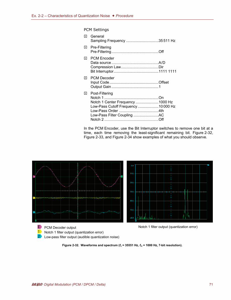
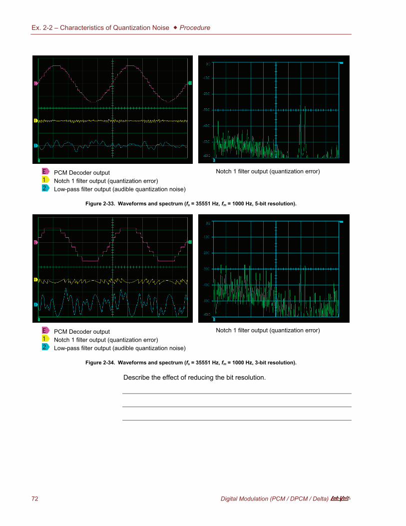
In the PCM Encoder, use the Bit Interruptor switches to remove one bit at a time, each time removing the least-significant remaining bit. Figure 2-32, Figure 2-33, and Figure 2-34 show examples of what you should observe.
PCM Decoder output Notch 1 filter output (quantization error) Low-pass filter output (audible quantization noise)
Notch 1 filter output (quantization error)
Figure 2-32.�Waveforms and spectrum (fs = 35551 Hz, fm = 1000 Hz, 7-bit resolution).
Ex. 2-2 – Characteristics of Quantization Noise � Procedure
72 Digital Modulation (PCM / DPCM / Delta)
PCM Decoder output Notch 1 filter output (quantization error) Low-pass filter output (audible quantization noise)
Notch 1 filter output (quantization error)
Figure 2-33.�Waveforms and spectrum (fs = 35551 Hz, fm = 1000 Hz, 5-bit resolution).
PCM Decoder output Notch 1 filter output (quantization error) Low-pass filter output (audible quantization noise)
Notch 1 filter output (quantization error)
Figure 2-34.�Waveforms and spectrum (fs = 35551 Hz, fm = 1000 Hz, 3-bit resolution).
Describe the effect of reducing the bit resolution.
Ex. 2-2 – Characteristics of Quantization Noise � Procedure
Digital Modulation (PCM / DPCM / Delta) 73
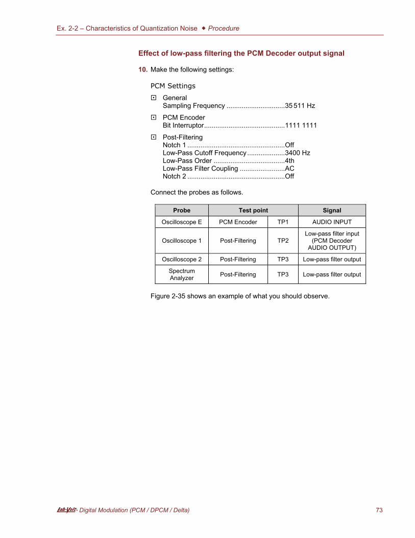
Effect of low-pass filtering the PCM Decoder output signal
10. Make the following settings:
PCM Settings
� General Sampling Frequency ............................... 35 511 Hz
� PCM Encoder Bit Interruptor ........................................... 1111 1111
� Post-Filtering Notch 1 .................................................... Off Low-Pass Cutoff Frequency .................... 3400 Hz Low-Pass Order ...................................... 4th Low-Pass Filter Coupling ........................ AC Notch 2 .................................................... Off
Connect the probes as follows.
Probe Test point Signal
Oscilloscope E PCM Encoder TP1 AUDIO INPUT
Oscilloscope 1 Post-Filtering TP2 Low-pass filter input
(PCM Decoder AUDIO OUTPUT)
Oscilloscope 2 Post-Filtering TP3 Low-pass filter output
Spectrum Analyzer Post-Filtering TP3 Low-pass filter output
Figure 2-35 shows an example of what you should observe.
Ex. 2-2 – Characteristics of Quantization Noise � Procedure
74 Digital Modulation (PCM / DPCM / Delta)
PCM Encoder AUDIO INPUT (message signal PCM Decoder AUDIO OUTPUT Low-pass filter output (reconstructed signal)
Low-pass filter output (reconstructed signal)
Figure 2-35.�Waveforms and spectrum (fs = 35551 Hz, fm = 1000 Hz, 8-bit resolution).
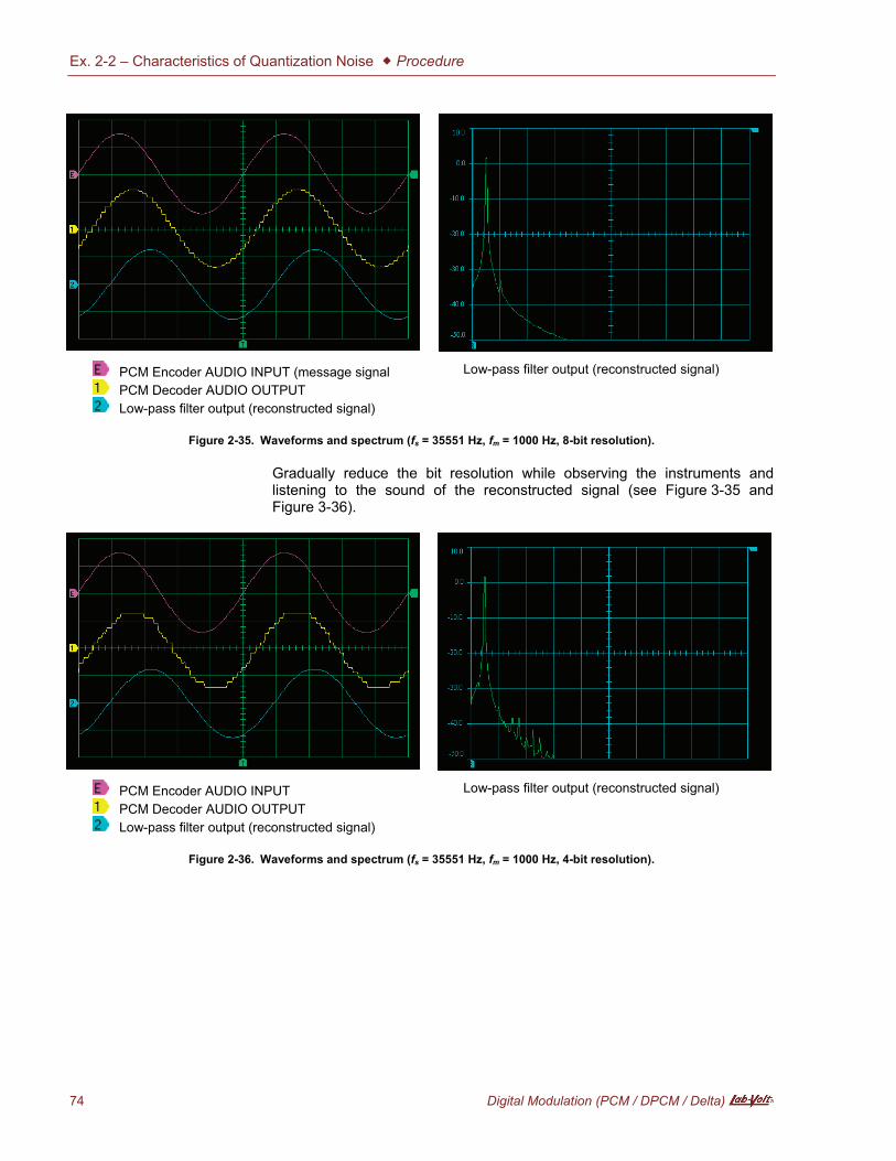
Gradually reduce the bit resolution while observing the instruments and listening to the sound of the reconstructed signal (see Figure 3-35 and Figure 3-36).
PCM Encoder AUDIO INPUT PCM Decoder AUDIO OUTPUT Low-pass filter output (reconstructed signal)
Low-pass filter output (reconstructed signal)
Figure 2-36.�Waveforms and spectrum (fs = 35551 Hz, fm = 1000 Hz, 4-bit resolution).
Ex. 2-2 – Characteristics of Quantization Noise � Procedure
Digital Modulation (PCM / DPCM / Delta) 75
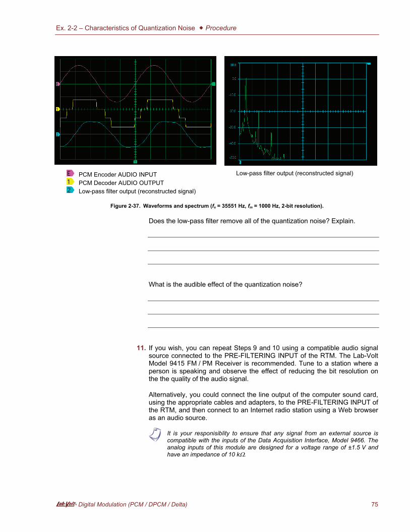
PCM Encoder AUDIO INPUT PCM Decoder AUDIO OUTPUT Low-pass filter output (reconstructed signal)
Low-pass filter output (reconstructed signal)
Figure 2-37.�Waveforms and spectrum (fs = 35551 Hz, fm = 1000 Hz, 2-bit resolution).
Does the low-pass filter remove all of the quantization noise? Explain.
What is the audible effect of the quantization noise?
11. If you wish, you can repeat Steps 9 and 10 using a compatible audio signal source connected to the PRE-FILTERING INPUT of the RTM. The Lab-Volt Model 9415 FM / PM Receiver is recommended. Tune to a station where a person is speaking and observe the effect of reducing the bit resolution on the the quality of the audio signal.
Alternatively, you could connect the line output of the computer sound card, using the appropriate cables and adapters, to the PRE-FILTERING INPUT of the RTM, and then connect to an Internet radio station using a Web browser as an audio source.
a It is your responisiblity to ensure that any signal from an external source is compatible with the inputs of the Data Acquisition Interface, Model 9466. The analog inputs of this module are designed for a voltage range of ±1.5 V and have an impedance of 10 k�.
Ex. 2-2 – Characteristics of Quantization Noise � Conclusion
76 Digital Modulation (PCM / DPCM / Delta)
12. When you have finished using the system, exit the LVCT software and turn off the equipment.
In this exercise, you observed quantization error in the time domain and in the frequency domain. In the time domain, you showed the effect of the sampling frequency on the quantization error waveform. You learned that quantization noise decreases when the number of quantization intervals is increased. You also observed the broad bandwidth of quantization noise and how it can be reduced by increasing the number of quantization intervals. You further observed that quantization noise cannot be totally eliminated by low-pass filtering the output of the PCM Decoder.
1. Explain how quantization noise arises.
2. For a given sampling rate, how can quantization noise be reduced?
3. Why does the quantization noise get worse when you use a lower sampling rate to quantize a sine wave?
4. What effect does a low-pass filter have on quantization noise?
CONCLUSION
REVIEW QUESTIONS
Ex. 2-2 – Characteristics of Quantization Noise � Review Questions
Digital Modulation (PCM / DPCM / Delta) 77
5. What does quantization noise sound like with a 6-, 7-, or 8-bit PCM system?

Other Sample
Extracted from
Digital Modulation
(PCM / DPCM / Delta)

Unit 2 – Distortion and Quantization Noise � Unit Test
Digital Modulation (PCM / DPCM / Delta) 91
Unit Test
1. The signal-to-quantization noise ratio for a PCM system
a. decreases as the message signal amplitude increases. b. is not affected by the amplitude of the message signal. c. increases as the message signal amplitude increases. d. none of the above.
2. The signal-to-noise ratio is defined as:
a. the ratio of the average signal power to the average noise power. b. the ratio of the signal voltage to the noise voltage. c. the ratio of the signal power in dB to the noise power in dB. d. none of the above.
3. Aliasing occurs
a. when using flat-top sampling. b. when the sampling rate is less than the Nyquist rate. c. when the message signal contains a large number of frequency
components. d. when the sampling rate is greater than the Nyquist rate.
4. Aliasing distortion
a. is enhanced by low-pass prefiltering. b. can be eliminated by low-pass prefiltering. c. can be reduced by low-pass prefiltering. d. is not affected by low-pass prefiltering.
5. Aperture distortion
a. can be corrected by an equalizing filter. b. boosts the low frequency components of a message signal. c. attenuates the high frequency components of a message signal. d. both a and c.
6. Aperture distortion is caused by
a. sampling at a rate greater than the Nyquist rate. b. the occurrence of sunspots. c. the shape of the sampling signal's frequency spectrum. d. all of the above.
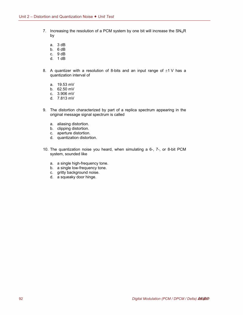
Unit 2 – Distortion and Quantization Noise � Unit Test
92 Digital Modulation (PCM / DPCM / Delta)
7. Increasing the resolution of a PCM system by one bit will increase the SNQR by
a. 3 dB b. 6 dB c. 9 dB d. 1 dB
8. A quantizer with a resolution of 8-bits and an input range of �1 V has a quantization interval of
a. 19.53 mV b. 62.50 mV c. 3.906 mV d. 7.813 mV
9. The distortion characterized by part of a replica spectrum appearing in the original message signal spectrum is called
a. aliasing distortion. b. clipping distortion. c. aperture distortion. d. quantization distortion.
10. The quantization noise you heard, when simulating a 6-, 7-, or 8-bit PCM system, sounded like
a. a single high-frequency tone. b. a single low-frequency tone. c. gritty background noise. d. a squeaky door hinge.
Instructor Guide
Sample Exercise
Extracted from
Digital Modulation
(PCM / DPCM / Delta)

Exercise 2-2 Characteristics of Quantization Noise
12 Digital Modulation (PCM / DPCM / Delta)
Exercise 2-2 Characteristics of Quantization Noise
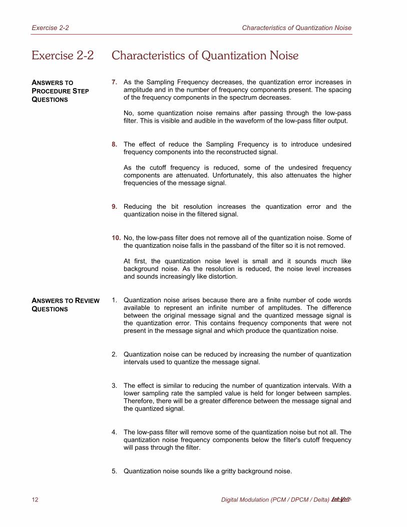
7. As the Sampling Frequency decreases, the quantization error increases in amplitude and in the number of frequency components present. The spacing of the frequency components in the spectrum decreases.
No, some quantization noise remains after passing through the low-pass filter. This is visible and audible in the waveform of the low-pass filter output.
8. The effect of reduce the Sampling Frequency is to introduce undesired frequency components into the reconstructed signal.
As the cutoff frequency is reduced, some of the undesired frequency components are attenuated. Unfortunately, this also attenuates the higher frequencies of the message signal.
9. Reducing the bit resolution increases the quantization error and the quantization noise in the filtered signal.
10. No, the low-pass filter does not remove all of the quantization noise. Some of the quantization noise falls in the passband of the filter so it is not removed.
At first, the quantization noise level is small and it sounds much like background noise. As the resolution is reduced, the noise level increases and sounds increasingly like distortion.
1. Quantization noise arises because there are a finite number of code words available to represent an infinite number of amplitudes. The difference between the original message signal and the quantized message signal is the quantization error. This contains frequency components that were not present in the message signal and which produce the quantization noise.
2. Quantization noise can be reduced by increasing the number of quantization intervals used to quantize the message signal.
3. The effect is similar to reducing the number of quantization intervals. With a lower sampling rate the sampled value is held for longer between samples. Therefore, there will be a greater difference between the message signal and the quantized signal.
4. The low-pass filter will remove some of the quantization noise but not all. The quantization noise frequency components below the filter's cutoff frequency will pass through the filter.
5. Quantization noise sounds like a gritty background noise.
ANSWERS TO PROCEDURE STEP QUESTIONS
ANSWERS TO REVIEW QUESTIONS

Bibliography
BELLAMY, John C., Digital Telephony, New York, John Wiley & Sons, 1982.ISBN 0-471-08089-6
FONTOLLIET, Pierre-Gerard, Telecommunication Systems, Deadham, Mass.,Artech House, 1986.
ISBN 0-89006-184-X
HAYKIN, Simon, Communication Systems, New York, John Wiley & Sons, 1978.ISBN 0-471-02977-7
OWEN, Frank F.E., PCM and Digital Transmission Systems, New York, Mc GrawHill,1982.
ISBN 0-07-047954-2
SHANMUGAM, K. Sam, Digital and Analog Communication Systems, New York,John Wiley & Sons, 1979.
ISBN 0-471-03090-2
SINNEMA, William, Digital, Analog, and Data Communication, Second Edition,Englewood Cliffs, New Jersey, Prentice-Hall, 1986.
ISBN 0-8359-1301-5
SMITH, David R., Digital Transmission Systems, New York, Van Nostrand Reinhold,1985.
ISBN 0-534-03382-2
STREMLER, Ferrel G., Introduction to Communication Systems, Second Edition,Reading, Mass., Addison-Wesley, 1982.
ISBN 0-201-07251-3


![Chapter-3 - ajaybolar.weebly.com · Chapter-3 . Waveform Coding Techniques . PCM [Pulse Code Modulation] PCM is an important method of analog -digital conversion. In this modulation](https://img.pdfslide.us/doc/110x75/5e0ec414f5a39e518c0f100c/chapter-3-chapter-3-waveform-coding-techniques-pcm-pulse-code-modulation.jpg)