Euro. Jnl of Applied Mathematics (2002), vol. 13, pp. 353–370. c© 2002 Cambridge University Press

DOI: 10.1017/S0956792501004904 Printed in the United Kingdom

353

Digital inpainting based on theMumford–Shah–Euler image model

SELIM ESEDOGLU1 and JIANHONG SHEN2

1 Institute of Mathematics and its Applications (IMA), University of Minnesota, Minneapolis, MN 55455, USA

email: esedoglu@ima.umn.edu2 School of Mathematics, University of Minnesota, Minneapolis, MN 55455, USA

email: jhshen@math.umn.edu

(Received 15 January 2002; revised 5 February 2002)

Image inpainting is an image restoration problem, in which image models play a critical

role, as demonstrated by Chan, Kang & Shen’s [12] recent inpainting schemes based on

the bounded variation and the elastica [11] image models. In this paper, we propose two

novel inpainting models based on the Mumford–Shah image model [41], and its high order

correction – the Mumford–Shah–Euler image model. We also present their efficient numerical

realization based on the Γ -convergence approximations of Ambrosio & Tortorelli [2, 3] and

De Giorgi [21].

1 Introduction

Inpainting is the process of filling in the missing or desired image information on domains

where it is unavailable (see Figure 1). Such ‘blank’ domains may be introduced by the

scratches in a photograph, the aging of the canvas and oil of an ancient painting, the

occlusion by undesired objects in front of a scene of interest, etc.

Initially motivated by the manual retouching work of museum artists [19, 48], as first

appeared in the pioneering work of Bertalmio et al. [7], digital inpainting has found its

wide application in image processing, vision analysis, and the movie industry. Recent

examples include: automatic scratch removal in digital photos and old films [7, 12], text

erasing [5, 7, 12, 14], special effects such as object disappearance [7, 14], disocclusion [37],

spatial/temporal zooming and super-resolution [5, 12, 47], lossy perceptual image co-

ding [12], and removal of the laser dazzling effect [18], and so on. On the other hand,

in the engineering literature, there also have been many earlier works closely related

to inpainting, which include image interpolation [4, 28, 29], image replacement [24, 49]

and error concealment [16, 25, 30] in communication technology. As scattered as the

applications are, the methods for the inpainting related problems have also been very

diversified, including the nonlinear filtering method, the Bayesian method, wavelets and

spectral method, and the learning-and-growing method (especially for textures) (see, for

example, recent work [1, 9, 24, 32, 49]).

The most recent approach to (non-texture) inpainting is based on the PDE method and

Calculus of Variations, and can be classified into two categories. The first class is based

354 S. Esedoglu and J. Shen

0

D

Dc is given

(inpainting domain)

u

Figure 1. For a typical inpainting problem, the image is missing on the inpainting domain D, and

the available part u0|Dc is often noisy.

on the simulation of micro-inpainting mechanisms. It includes the axiomatic approach

of Caselles et al. [10], the transportation process [7] (the first high-order PDE model),

the diffusion process [14], and their combination [6, 13]. The second category includes all

variational models simulating the unique macro-inpainting mechanism: ‘best guess’, or the

Bayesian framework [20, 27, 40]. The latter includes the total variation model [15, 12, 44,

45], the functionalized elastica model [11, 37], the value-and-direction joint model [5], and

the active contour model based on Mumford and Shah’s segmentation [47]. The Bayesian

view on this category is also explained in the recent work of Chan et al. [11], and the

underlying philosophy is indeed simple and intuitive: the way we (human inpainters)

inpaint an incomplete picture mostly depends on two factors – how we read the existing

part of the picture (i.e. the data model), and what class of images we believe the picture

belongs to (i.e. the image model). For the latter, for example, most windows and buildings

have rectangular outlines, while tomatoes, potatoes, apples, and bottles in a kitchen are

mostly round and smooth [42]. Such prior knowledge (or image model) is crucial for

effectual inpainting.

The present work belongs to the latter category, and is intended to contribute to the

further development of a key idea that first appeared in the recent works of Chan &

Shen [12], and Tsai et al. [47].

We propose two inpainting schemes based on the Mumford–Shah image model [41],

and its high-order correction, the Mumford–Shah–Euler image model. The latter improves

the former by replacing the embedded straight-line curve model with Euler’s elastica [33].

Euler’s elastica was first introduced by Mumford [39] into computer vision as a curve

model, and has recently found its effective application in image inpainting through direct

functionalization [11, 37].

The news about inpainting based on the Mumford–Shah image model (as first proposed

in Chan & Shen [12] and Tsai et al. [47]) is mixed. The positive side is its lower order of

complexity in terms of approximation and computation (§ 2). But unlike its effectiveness

in the conventional application of segmentation and denoising (March & Dozio [34, 35]

and Chan & Vese [17], for example), the Mumford–Shah image model has its inherent

deficiency for inpainting, as will be explained in § 3 through two typical examples. The

inpainting model based on the Mumford–Shah–Euler image model is designed to remedy

such deficiency, and produce more natural visual effect (§ 4).

To turn these models to practical digital schemes, we seek help from the Γ -convergence

results of Ambrosio & Tortorelli [2, 3] for the Mumford–Shah image model, and a

conjecture of De Giorgi [21] for Euler’s elastica. We explain why the Γ -convergence

Inpainting via the Mumford–Shah–Euler image model 355

approximations appear to be more natural for inpainting than for segmentation and

denoising. We also discuss the stable and efficient numerical implementation of the elliptic

systems derived from these approximate models, as inspired by March & Dozio’s [34, 35]

similar earlier work on segmentation. These are discussed in § 2 and § 4.

Parallel to the level-set formulation in Chan & Shen [12] and Tsai et al. [47] for

Mumford–Shah segmentation, in § 4, we present the level-set formulation for inpainting

based on the Mumford–Shah–Euler image model, and discuss some related computational

issues. § 5 contains a brief summary and conclusion.

Throughout this paper, Ω denotes the entire image domain (in R2), x ∈ Ω a general

pixel, D the inpainting domain where the image is missing, and u0 the available part of

the image on Ω\D. For any multi-variable function or functional F(X,Y ), the symbol

F(X|Y ) still means F(X,Y ), but with Y fixed as known. This is by analogy with conditional

probability or expectation in probability theory (but without normalization).

It is our best wish, that the current work, together with the efforts of all the authors

whose works have been just mentioned, can generate further attention and interest from

the applied mathematics community.

2 Inpainting via Mumford–Shah image model

A general variational inpainting model is to minimize an appropriate ‘energy’ functional

J[u|u0, D] or J[u|u0 given on Ω\D].

By the Bayesian rationale [40], the energy consists of two parts:

J[u|u0, D] =λ

2

∫Ω\D

(u− u0)2 + E[u], (2.1)

where E[u] encodes the image model, and the first term expresses the data model, of

which we have assumed that

u0 = uoriginal + Gaussian white noise n.

Define λD(x) = λ · 1Ω\D(x). Then the data model can be written as

1

2

∫Ω

λD(x)(u− u0)2dx.

The image model that Mumford & Shah [41] proposed for segmentation is the object-edge

model:

E[u, Γ ] =γ

2

∫Ω\Γ|∇u|2dx+ αH1(Γ ), (2.2)

where Γ denotes the edge collection, H1 the one dimensional Hausdorff measure, which

generalizes the notion of length for regular curves. In fact, in most segmentation applica-

tions, especially in numerical computation [17, 47], H1(Γ ) is conveniently substituted by

length(Γ ), under the assumption that Γ belongs to the Lipschitz class.

Therefore, by (2.1), inpainting based on the Mumford–Shah image model is to minimize

Jms[u, Γ |u0, D] =1

2

∫Ω

λD(u− u0)2dx+γ

2

∫Ω\Γ|∇u|2dx+ αH1(Γ ). (2.3)

356 S. Esedoglu and J. Shen

The idea first appeared in the recent works of Tsai et al. [47] and Chan & Shen [12].

In Chan & Shen [12] it was introduced as an alternative to the TV inpainting model. In

Tsai et al. [47] it serves as one of the major examples and applications for the numerical

active contour algorithm.

In this section, we propose to apply the Γ -convergence approximation of E[u, Γ ] to

inpainting (2.3), as initially studied by Ambrosio and Tortorelli in the context of im-

age segmentation. We shall explain why such an approximation becomes more ideal for

inpainting than for the original segmentation task. More importantly, the Ambrosio–

Tortorelli approximation leads to a very simple inpainting algorithm, and its rapid

numerical convergence.

In the Ambrosio–Tortorelli’s Γ -convergence approximation, the edge set Γ is approxi-

mated by its ‘signature’ function zε:

zε : Ω → [0, 1],

which is nearly 1 almost everywhere except on a tiny tubular neighbourhood (with width

O(ε)) of Γ , where it is close to 0. Thus, up to a multiplicative normalization factor of

order O(1),

1

ε|1− zε|p, p > 1,

is an approximation to the Dirac delta measure of Γ — δΓ (x):∫Ω

δΓ (x)f(x)dx =

∫Γ

f(x(s))ds,

where s is the arc-length parameter. Therefore,

length(Γ ) =

∫Ω

δΓ (x)dx = const.

∫Ω

|1− zε|pε

dx.

In fact, in Ambrosio & Tortorelli’s [2, 3] approximation, p is taken to be 2, and z = zεis designed to minimize

Eε[z|u] =γ

2

∫Ω

z2|∇u|2dx+ α

∫Ω

(ε|∇z|2 +

(1− z)2

4ε

)dx (2.4)

(by Ambrosio & Tortorelli [2, 3], z2 should be z2 + o(ε).) Compared with the original

image model (2.2), this is based on two (coupled) approximations (up to a multiplicative

constant of order one) ∫Ω\Γ|∇u|2dx '

∫Ω

z2|∇u|2dx

length(Γ ) '∫Ω

(ε|∇z|2 +

(1− z)2

4ε

)dx.

The disadvantage of the approximation is that the edges in the image are represented by

diffuse interfaces as opposed to sharp ones. As mentioned above, the transition bandwidth

of the edge signature z is of order ε. Even though ε needs to be small in theory, the

Inpainting via the Mumford–Shah–Euler image model 357

numerical grid size imposes a lower bound – we found that for a reliable approximation

and a stable scheme, the transition band must be sufficiently resolved. As a result,

numerically feasible ε’s lead to quite diffuse transitions and increase the uncertainty of

the edge locations.

However, the enormous gain of the approximate model lies in that it is a quadratic

integral of z and u, and can be easily solved numerically using either the finite element or

the finite difference methods (see March [34], for example).

For segmentation, the disadvantage can sometimes be influential, since high resolution

of the edge layout is indeed needed (such as in the disocclusion application of Nitzberg

et al. [42], and for accurately estimating the growth rate of a certain species of cells under

a fixed microscopic view in medical image processing). For inpainting, however, the only

concern is the restored image u, not the edge signature z. The low resolution of the edge

set presented by z has little influence on the restored image u. The sharpness of the real

edges of u is well preserved as long as z almost vanishes along a narrow band covering the

real edges. This makes the Ambrosio–Tortorelli approximation more ideal for inpainting.

It leads to simple and fast computational schemes without losing the inpainting quality.

Another notable advantage over the level-set algorithm is that the z function makes it

unnecessary to assign multiphase level-set functions, or equivalently, it does not need to

deal with the four-color problem mentioned in Chan & Vese [17].

In summary, we propose to carry out inpainting by minimizing the Γ -convergence

approximation of the exact model (2.3), namely

Jε[u, z|u0, D] =1

2

∫Ω

λD(x)(u− u0)2dx+γ

2

∫Ω

z2|∇u|2dx+ α

∫Ω

(ε|∇z|2 +

(1− z)2

4ε

)dx.

(2.5)

Taking variations on u and z separately yields the Euler–Lagrange system,

λD(x)(u− u0)− γ∇ · (z2∇u) = 0 (2.6)

(γ|∇u|2)z + α

(−2ε∆z +

z − 1

2ε

)= 0, (2.7)

with the natural adiabatic boundary conditions (due to the boundary integrals coming

from integration-by-parts):

∂u

∂~n= 0,

∂z

∂~n= 0. (2.8)

Define two differential operators acting on u and z separately:

Lz = −∇ · z2∇+ λD/γ, (2.9)

Mu = (1 + 2(εγ/α)|∇u|2)− 4ε2∆. (2.10)

Given a pair of the current estimation u and z, both Lz and Mu are positive definite elliptic

operators. (Note: Lz is indeed positive definite since in both theory and computation [2, 3],

z2 is replaced by z2 + c, where c is a positive constant decaying faster than ε as ε → 0.)

The Euler–Lagrange system (2.6) and (2.7) is simply written as

Lzu = (λD/γ)u0 and Muz = 1. (2.11)

358 S. Esedoglu and J. Shen

Noisy image to be inpainted Inpainting output u Inpainting output z

Figure 2. Inpainting based on the Γ -convergence approximation (2.5) and its associated elliptic

system (2.11). The annular inpainting domain is initially inpainted with a random guess for the

iterative strategy (2.12) or (2.13).

Image to be inpainted Inpainting domain (or mask) Inpainting output

Figure 3. Automatic text erasing by the inpainting model based on the Γ -convergence

approximation (2.5) and (2.11).

This coupled system can be solved easily by any efficient elliptic solver and an iterative

scheme such as the sequential strategy:

Lz(n−1)u(n) = (λD/γ)u0 and Mu(n)z(n) = 1, (2.12)

and the parallel strategy:

Lz(n−1)u(n) = (λD/γ)u0 and Mu(n−1)z(n) = 1. (2.13)

Compared with March’s approach for segmentation [34], this scheme is more stable and

converges faster.

We have included in this section two numerical examples based on model (2.5) and

its associated elliptic system (2.11). Figure 2 is a typical example in the inpainting

literature [7, 12], of which the inpainting domain has a complicated topology (e.g. non-

convex and not simply connected). The advantage of the numerical PDE approach,

as compared with the dynamic programming algorithm of Masnou & Morel [37], is its

capability of automatic filling regardless the shape and topology of the inpainting domain.

The second example in Figure 3 shows an application of the inpainting technique for

automatic text erasing.

Inpainting via the Mumford–Shah–Euler image model 359

Segmenting

Inpainting

Figure 4. The Mumford–Shah image model works well for segmentation (top row), but produces

visible artificial corners when applied to inpainting (bottom row), due to the lack of balance from

the data model (or the fidelity term) on the missing domain (§ 3.1).

3 Why is Mumford–Shah insufficient for inpainting?

Numerous publications and numerical experiments ([17, 34, 47], to name a few) have

demonstrated the power of the Mumford–Shah image model for image segmentation

and denoising. In this section, however, we discuss its insufficiency for inpainting. The

shortcomings are first discovered by Chan & Shen [12], and are parallel to those of the

TV inpainting model [12].

In Mumford and Shah’s object-edge image model,

E[u, Γ ] =γ

2

∫Ω\Γ|∇u|2dx+ α length(Γ ),

the preferable edge curves are those which have the shortest length. Therefore, without

other types of constraints, it favours straight edges. In the classical segmentation and

denoising application, the straight-line curve model is well balanced by the data model

(or the fidelity term)

λ

2

∫Ω

(u− u0)2dx.

For example, we are still able to observe smoothly curved edges for blood cells in medical

image processing, or for images with apples or tomatoes (check the top row of Figure 4).

The situation changes for inpainting, of which the image model is solely responsible for

the reconstruction on the inpainting domain D. We explain the resulting defects through

two typical phenomena and examples in the inpainting literature.

3.1 Emerging of artificial corners

The first artifact is the emerging of artificial corners, as clearly visible in Figure 4.

Due to the lack of balance from the data model on the inpainting domain (the square

domain in the bottom row, initially inpainted with a random guess), model (2.3) (or its

approximation (2.5)) simply ‘draws’ a straight line to complete the missing edge segment,

since this costs the least energy according to the Mumford–Shah image model. As a

360 S. Esedoglu and J. Shen

Segmenting Inpainting ( l < w )

Inpainting ( l > w )

w

LL

w

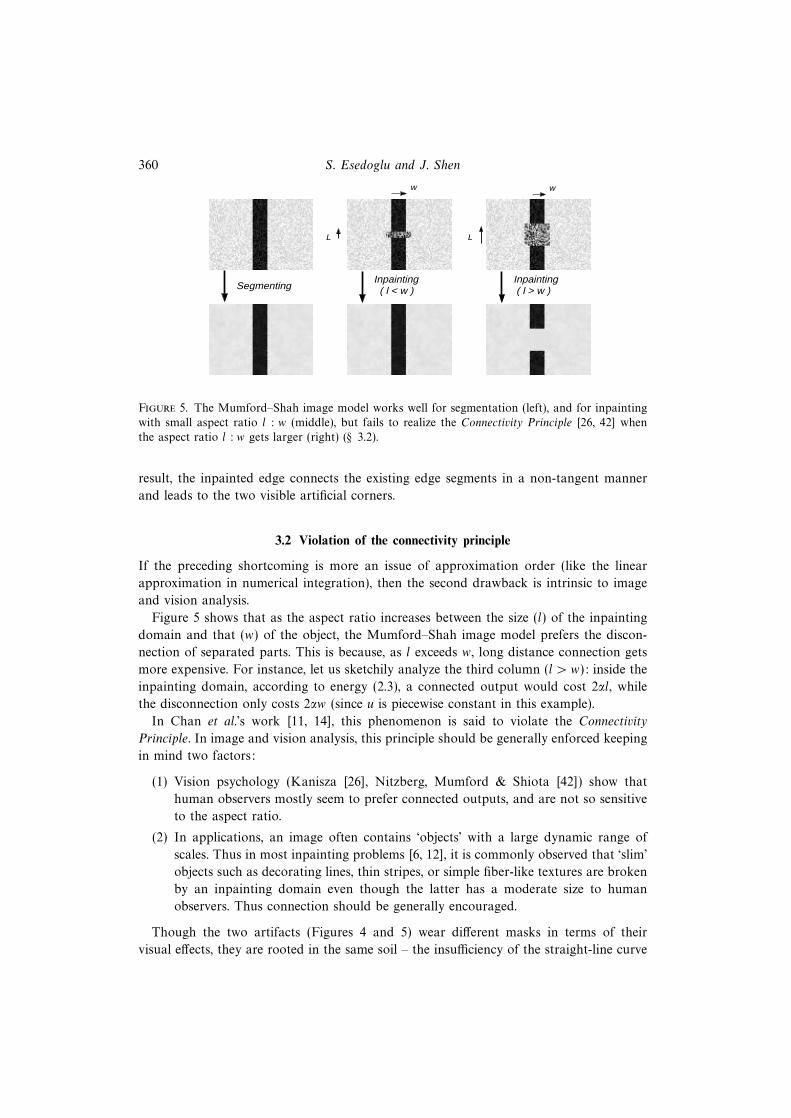
Figure 5. The Mumford–Shah image model works well for segmentation (left), and for inpainting

with small aspect ratio l : w (middle), but fails to realize the Connectivity Principle [26, 42] when

the aspect ratio l : w gets larger (right) (§ 3.2).

result, the inpainted edge connects the existing edge segments in a non-tangent manner

and leads to the two visible artificial corners.

3.2 Violation of the connectivity principle

If the preceding shortcoming is more an issue of approximation order (like the linear

approximation in numerical integration), then the second drawback is intrinsic to image

and vision analysis.

Figure 5 shows that as the aspect ratio increases between the size (l) of the inpainting

domain and that (w) of the object, the Mumford–Shah image model prefers the discon-

nection of separated parts. This is because, as l exceeds w, long distance connection gets

more expensive. For instance, let us sketchily analyze the third column (l > w): inside the

inpainting domain, according to energy (2.3), a connected output would cost 2αl, while

the disconnection only costs 2αw (since u is piecewise constant in this example).

In Chan et al.’s work [11, 14], this phenomenon is said to violate the Connectivity

Principle. In image and vision analysis, this principle should be generally enforced keeping

in mind two factors:

(1) Vision psychology (Kanisza [26], Nitzberg, Mumford & Shiota [42]) show that

human observers mostly seem to prefer connected outputs, and are not so sensitive

to the aspect ratio.

(2) In applications, an image often contains ‘objects’ with a large dynamic range of

scales. Thus in most inpainting problems [6, 12], it is commonly observed that ‘slim’

objects such as decorating lines, thin stripes, or simple fiber-like textures are broken

by an inpainting domain even though the latter has a moderate size to human

observers. Thus connection should be generally encouraged.

Though the two artifacts (Figures 4 and 5) wear different masks in terms of their

visual effects, they are rooted in the same soil – the insufficiency of the straight-line curve

Inpainting via the Mumford–Shah–Euler image model 361

model embedded within the Mumford–Shah image model (2.2). Our next image model

thus incorporates an improved curve model – Euler’s elastica [11, 39], and is called the

Mumford–Shah–Euler image model for the ease of reference.

Finally, we must point out that, despite the artifacts that the Mumford–Shah image

model may produce, it is still an attractive one for digital inpainting due to the lower

complexity of the associated differential equations and their fast computational schemes. It

can at least supply high-quality initial guesses for computationally more costly inpainting

schemes. On the other hand, for the recent novel applications in digital zooming and

super-resolution [12], such lower order model is indeed already sufficient due to the local

nature of these problems.

4 Inpainting via Mumford–Shah–Euler image model

As concluded from the discussion, the key to remedying the insufficiency of the Mumford–

Shah image model is to improve its embedded curve model. As initially introduced into

computer vision by Mumford [39], Euler’s elastica curve model

e(Γ ) =

∫Γ

(α+ βκ2)ds = α length(Γ ) + β

∫Γ

κ2ds (4.1)

is a high order correction to the straight-line one. Here κ denotes the curvature, ds the

length element, and α and β two tunable positive weights. The energy was first studied

by Euler to model the shape of a thin and torsion-free rod [33]. In approximation theory,

Birkhoff & De Boor [8] referred to it as ‘nonlinear spline’ for data fitting or interpolation,

as compared to the classical polynomial based (linear) splines. Recently, Masnou &

Morel [37] and Chan et al. [11] ‘lifted’ the elastica curve model to an image model by

direct functionalization, and applied it to disocclusion and image inpainting.

We shall call the modified energy

E[u, Γ ] =γ

2

∫Ω\Γ|∇u|2dx+ e(Γ ) =

γ

2

∫Ω\Γ|∇u|2dx+

∫Γ

(α+ βκ2)ds (4.2)

the Mumford–Shah–Euler image model in this paper. The corresponding inpainting model

becomes

Jmse[u, Γ |u0, D] =1

2

∫Ω

λD(u− u0)2dx+γ

2

∫Ω\Γ|∇u|2dx+

∫Γ

(α+ βκ2)ds. (4.3)

For a given edge layout Γ , the Euler–Lagrange equation for Jmse[u|Γ , u0, D] is

λD(x)(u0 − u) + γ∆u = 0, x ∈ Ω\Γ , (4.4)

with the adiabatic condition along Γ and ∂Ω: ∂u/∂~n = 0. For the solution u, the Euler–

Lagrange equation for Jmse[Γ |u, u0, D] can be worked out to be [11, 39, 31][γ

2|∇u|2 +

λD

2(u− u0)2

]Γ

+ ακ− β(

2d2κ

ds2+ κ3

)= 0, (4.5)

where, given an arbitrary orientation (i.e. tangent direction~t) of Γ , κ = |d~t/ds| (and thus

d~t/ds = κ~n) is the curvature, and [φ]Γ denotes the jump of a scalar function φ across the

362 S. Esedoglu and J. Shen

normal direction ~n: for any x ∈ Γ ,

[φ]Γ (x) = limε→0+

(φ(x+ ε~n)− φ(x− ε~n)).For simplicity, we have assumed that the edge layout Γ is smooth enough.

Computationally, the elliptic equation (4.4) for updating u can be easily solved. The

curve equation (4.5), on the other hand, leads to the active contour evolution:

dx

dt=

(ακ− β

(2d2κ

ds2+ κ3

)+

[γ

2|∇u|2 +

λD

2(u− u0)2

]Γ

)~n. (4.6)

Due to the presence of the curvature term and its second derivative, the numerical

implementation of (4.6) is much more involved than the conventional mean curvature

motion. In what follows, we discuss two approaches: the level-set method of Osher &

Sethian [43], and the method similar to § 2 based on the Γ -convergence approximation

conjecture of De Giorgi [21].

4.1 The level-set formulation of Osher and Sethian

Here we present the level-set method for a two-phase situation. The recent work of Chan

& Vese [17] contains a detailed explanation of the multi-phase level-set method for the

Mumford–Shah segmentation model.

In the level-set formulation of Osher & Sethian [43], the edge layout Γ is embedded

as the zero level-set of a Lipschitz continuous function φ(x): Γ = x : φ(x) = 0. This

redundant representation is then trimmed by the Heaviside functions

H+(φ) =

1 φ > 0

0 φ 6 0and H−(φ) =

1 φ < 0

0 φ > 0.

Both numerically and theoretically, they are understood as the distributional limit (as ε

tends to 0+) of

Hε(φ) =

1 φ > ε

0 φ 6 εand H−ε(φ) =

1 φ < −ε0 φ > −ε .

Then the Mumford–Shah–Euler image model (4.2) has a natural representation under the

level-set function φ. First,∫Ω\Γ|∇u|2dx =

∫Ω

H+(φ)|∇u|2dx+

∫Ω

H−(φ)|∇u|2dx. (4.7)

For the elastica curve model, according to the similar idea of the co-area formula in the

space of bounded variations [22], we have (as applied to the BV function H+(φ)),∫Γ

(α+ βκ2)ds =

∫Ω

(α+ β

(∇ ·[ ∇H+(φ)

|∇H+(φ)|])2

)|∇H+(φ)|dx

=

∫Ω

(α+ β

(∇ ·[ ∇φ|∇φ|

])2)|∇φ|δ(φ)dx.

(4.8)

Here δ is the 1-D Dirac delta function, and the derivatives are understood formally, or in

Inpainting via the Mumford–Shah–Euler image model 363

the weak-limit sense via the Gaussian convolution (denoted by ∗) kernel Gσ(x):

∂

∂xi= lim

σ→0+

∂

∂xi Gσ∗,

for i = 1, 2. In numerical implementation, as Chan & Vese [17] practiced, the Dirac delta

function is replaced by its ε- approximation δε, for example,

δε(s) =1

εg( sε

), s ∈ R, (4.9)

for any numerically friendly positive function g with a bell shape and normalized total

integral.

Therefore, the level-set representation of Jmse[u, Γ |u0, D] becomes Jmse[u, φ|u0, D] as

assembled from (4.7), (4.8), and the original fidelity term, which is now expressed by

1

2

∫Ω

λD(u− u0)2dx =1

2

∫Ω

H+(φ)λD(u− u0)2dx+1

2

∫Ω

H−(φ)λD(u− u0)2dx.

For a fixed level-set function φ, variation of Jmse[u|φ, u0, D] on u gives

λD(u0 − u±) + γ∆u± = 0, on ± φ > 0,

separately for u± with the adiabatic boundary condition: ∂u±/∂~n = 0. Then the combi-

nation of the formulae in Chan et al. [11] and Chan & Vese [17] expresses the gradient

descent equation of J[φ|u±, u0, D] as

∂φ

∂t= δε(φ)

[∇ · ~V −

(γ

2(|∇u+|2 − |∇u−|2) +

λD

2((u+ − u0)2 − (u− − u0)2)

)], (4.10)

~V = (α+ βκ2)~n− 2β

|∇φ|∂(κ|∇φ|)

∂~t~t. (4.11)

Here

~n =∇φ|∇φ| , ~t =~n⊥,

∂

∂~t=~t · ∇, and κ = ∇ ·

[ ∇φ|∇φ|

].

(Note that, due to the parity of ~t in the formula, it makes no difference whether one

takes~t or −~t.)Since the numerical Dirac delta function δε has a non-zero bandwidth, to evolve φ

by (4.10), both u+ and u− have to be continuously extended across the edge set: Γ : φ = 0

(to at least cover the support of δε(φ(x)). Various computational techniques are available

to carry out the extension, as discussed in detail in Chan & Vese [17]. For the flux flow~V , one can benefit from the numerical (finite differencing) techniques described in Chan

et al. [11].

We refer to Chan & Vese’s recent work [17] for further detail regarding other compu-

tational issues such as the re-initialization process. Due to the less common fourth-order

(nonlinear) term related to the curvature, the level-set computation is however costly and

slow.

Thus, in the coming subsection, we seek an alternative computational strategy that

is based on the ‘elliptic’ approximation of the curvature term, as initially proposed by

De Giorgi [21].

364 S. Esedoglu and J. Shen

4.2 The Γ -convergence approximation conjecture of De Giorgi

De Giorgi [21, 35] proposed to approximate Euler’s elastica curve model

e(Γ ) =

∫Γ

(α+ βκ2)ds,

by the following integral of the signature z (α and β may be different):

Eε[z] = α

∫Ω

(ε|∇z|2 +

W (z)

4ε

)dx+

β

ε

∫Ω

(2ε∆z − W ′(z)

4ε

)2

dx, (4.12)

where W (z) can be the symmetric double-well function

W (z) = (1− z2)2 = (z + 1)2(z − 1)2. (4.13)

Unlike the choice of W (z) = (1− z)2 in the previous section of the Mumford–Shah image

model, here, more as in the level-set method, the edge layout Γ is embedded as the zero

level-set of z. Asymptotically, as ε → 0+, a boundary layer grows to realize the sharp

transition between the two well states z = 1 and z = −1.

As March & Dozio [35] did for segmentation, based on the De Giorgi approxima-

tion (4.12), we are able to replace the inpainting model (4.3) by an elliptic energy on u

and z:

Jε[u, z|u0, D] =1

2

∫Ω

λD(u− u0)2dx+γ

2

∫Ω

z2|∇u|2dx+ Eε[z], (4.14)

with Eε specified in (4.12). The remarkable difference between segmentation and inpainting

can be traced to the discussion in § 3. For segmentation, as March and Dozio practiced,

the ratio β : α can be as small as O(h2), with h denoting the distance between two nearest

neighbouring pixels. This is because, as clearly demonstrated in the top row of Figure 4,

even without the curvature term (i.e. the conventional Mumford–Shah model with β = 0),

the optimal edge layout can be as smooth as one expects, due to the balance of the

fidelity term. For inpainting, however, with the defects described in § 3 in mind, we have

to increase β to substantially enhance the role of the curvature term on the inpainting

domain. In fact, our numerical experiments suggest that β : α should be of order O(1).

Such large β dramatically increases numerical instability and thus restricts the stable size

of marching steps. It is a major computational barrier that one has to overcome for

realistic digital inpainting applications.

Let us work out the Euler–Lagrange system. For a given edge signature z, variation on

u in Jε[u|z, u0, D] gives

λD(u− u0)− γ∇ · (z2∇u) = 0, (4.15)

with the adiabatic boundary condition ∂u/∂~n = 0 along ∂Ω. Then the steepest descent

marching of z for Jε[z|u, u0, D] is given by (also see March & Dozio [35])

∂z

∂t= −γ|∇u|2z + αg +

βW ′′(z)2ε2

g − 4β∆g, (4.16)

g = 2ε∆z − W ′(z)4ε

, (4.17)

Inpainting via the Mumford–Shah–Euler image model 365

again with the Neumann adiabatic conditions along the boundary ∂Ω:

∂z

∂~n= 0, and

∂g

∂~n= 0.

Equation (4.16) is of fourth-order for z, with the leading term

−8εβ∆2z.

Thus, to ensure stability, an explicit marching scheme would require

∆t = O

((∆x)4

εβ

).

There are a couple of ways to stably increase the marching size. First, as inspired by

Marquina & Osher [36], one could add an automatic ‘time corrector’ T :

∂z

∂t= T (∇z, g|u)

(−γ|∇u|2z + αg +

βW ′′(z)2ε2

g − 4β∆g

),

where T (∇z, g, |u) is a suitable positive scalar, for example, T = |∇z|, as inspired by

the mean-curvature motion literature. The second alternative is to turn to implicit or

semi-implicit schemes. Equation (4.16) can be rearranged to

∂z

∂t+ γ|∇u|2z − 2αε∆z + 8βε∆2z = − α

4εW ′(z) +

βW ′′(z)2ε2

g +β

ε∆W ′(z), (4.18)

or simply

∂z

∂t+ Luz = f(z),

where Lu denotes the positive definite elliptic operator (u-dependent)

Lu = γ|∇u|2 − 2αε∆+ 8βε∆2,

and f(z) the entire right-hand side of (4.18). Then a semi-implicit scheme can be designed

as: at each discrete time step n,

(1 + ∆tLu)z(n+1) = z(n) + ∆tf(z(n)),

where the positive definite operator 1 + ∆tLu is numerically inverted based on many fast

solvers [23, 46].

Remarkably, the computational challenge does not end in the fourth order (4.10) or

(4.16). There is an extra layer of inherent difficulty with the inpainting model (4.3) – the

energy has many local minima! As in the notorious example of Molecular Dynamics

(MD) where the energy has too many local minima, the steepest-decent based marching

strategy (4.10) or (4.16), even if equipped with robust, stable, and efficient numerical

schemes, can be easily trapped and stagnate at the local energy ‘wells’. Such stagnation

can fail to carry out visually meaningful inpainting as discussed in § 3, for instance, the

failure to realize the Connectivity Principle.

This phenomenon does not bother much in segmentation and denoising. The reason

is similar to the discussion in § 3. For segmentation and denoising, the data model, or

equivalently, the fidelity term in the energy, confines all admissible inpaintings u within a

small ‘ball’ in L2(Ω) centered at u0, inside whose limited space, there are only one or very

366 S. Esedoglu and J. Shen

x

x

x

x

u0

u0|D

σ

σ

x

x

x

Global well

Local wells

trapped

Figure 6. Visualization of the difference between segmentation and inpainting (see the text

explanation).

A noisy image to be inpainted. Inpainting via Mumford−Shah−Euler image model

Figure 7. With Euler’s elastica curve model embedded inside, the inpainting model (4.3) based on

the Mumford–Shah–Euler image model is able to restore smoother missing edges and yield more

natural visual effect than the Mumford–Shah image model, as apparent from the comparison with

Figure 4.

few energy wells. However, for inpainting, we only know a ‘projection’ (in L2(Ω)) of the

entire image, and all admissible inpaintings u, despite the fidelity term, occupy an infinite

‘cylinder’ (in L2(Ω)), inside which the energy can have many energy wells. To visualize

this discussion, we have treated L2(Ω) as R3, and impressionistically plotted the situation

in Figure 6.

Therefore, in the subsequent future sibling work, we shall discuss in much detail and

more systematically how to computationally overcome such energy barriers. The potential

techniques include: Gaussian-smoothing (as in Molecular Dynamics [38]), the multireso-

lution approach (as in Tsai et al. [47]), the re-initialization or sharpening technique (as in

the level-set method of Osher & Sethian [43]), and the CDD technique (curvature driven

diffusion, as in Chan & Shen [14]).

We end this section by showing in Figures 7 and 8 two examples based on the

Mumford–Shah–Euler image models.

Inpainting via the Mumford–Shah–Euler image model 367

A noisy image to be inpainted. Inpainting by the Mumford−Shah−Euler image model

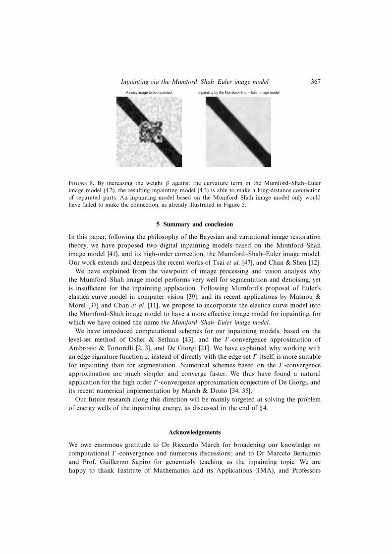
Figure 8. By increasing the weight β against the curvature term in the Mumford–Shah–Euler

image model (4.2), the resulting inpainting model (4.3) is able to make a long-distance connection

of separated parts. An inpainting model based on the Mumford–Shah image model only would

have failed to make the connection, as already illustrated in Figure 5.

5 Summary and conclusion

In this paper, following the philosophy of the Bayesian and variational image restoration

theory, we have proposed two digital inpainting models based on the Mumford–Shah

image model [41], and its high-order correction, the Mumford–Shah–Euler image model.

Our work extends and deepens the recent works of Tsai et al. [47], and Chan & Shen [12].

We have explained from the viewpoint of image processing and vision analysis why

the Mumford–Shah image model performs very well for segmentation and denoising, yet

is insufficient for the inpainting application. Following Mumford’s proposal of Euler’s

elastica curve model in computer vision [39], and its recent applications by Masnou &

Morel [37] and Chan et al. [11], we propose to incorporate the elastica curve model into

the Mumford–Shah image model to have a more effective image model for inpainting, for

which we have coined the name the Mumford–Shah–Euler image model.

We have introduced computational schemes for our inpainting models, based on the

level-set method of Osher & Sethian [43], and the Γ -convergence approximation of

Ambrosio & Tortorelli [2, 3], and De Giorgi [21]. We have explained why working with

an edge signature function z, instead of directly with the edge set Γ itself, is more suitable

for inpainting than for segmentation. Numerical schemes based on the Γ -convergence

approximation are much simpler and converge faster. We thus have found a natural

application for the high order Γ -convergence approximation conjecture of De Giorgi, and

its recent numerical implementation by March & Dozio [34, 35].

Our future research along this direction will be mainly targeted at solving the problem

of energy wells of the inpainting energy, as discussed in the end of § 4.

Acknowledgements

We owe enormous gratitude to Dr Riccardo March for broadening our knowledge on

computational Γ -convergence and numerous discussions; and to Dr Marcelo Bertalmio

and Prof. Guillermo Sapiro for generously teaching us the inpainting topic. We are

happy to thank Institute of Mathematics and its Applications (IMA), and Professors

368 S. Esedoglu and J. Shen

Willard Miller, Peter Olver and Fadil Santosa for their support during this project. In

addition, Selim Esedoglu benefited immensely from his recent visit to IAC in Rome, and

would also like to thank his former advisor Robert V. Kohn for continuing support and

encouragement. Jianhong (Jackie) Shen would like to thank all the following people for

making the ‘vision’ of the current paper possible: Professors Gilbert Strang, Tony Chan,

Stan Osher, Lumi Vese, Sung-Ha Kang, Li-Tien Cheng, Dan Kerstan, David Mumford,

Jean-Michel Morel, Stu Geman, Bob Gulliver, Rachid Deriche, Jin Keun Seo and the

Institute of Pure and Applied Mathematics (IPAM) at UCLA.

References

[1] Aldroubi, A. & Grochenig, K. (2001) Nonuniform sampling and reconstruction in shift-

invariant spaces. SIAM Rev. 43(4), 585–620.

[2] Ambrosio, L. & Tortorelli, V. M. (1990) Approximation of functionals depending on jumps

by elliptic functionals via Γ -convergence. Comm. Pure Appl. Math. 43, 999–1036.

[3] Ambrosio, L. & Tortorelli, V. M. (1992) On the approximation of free discontinuity problems.

Boll. Un. Mat. Ital. 6-B, 105–123.

[4] Armstrong, S., Kokaram, A. & Rayner, P. J. W. (1997) Nonlinear interpolation of missing

data using min-max functions. IEEE Int. Conf. Nonlinear Signal and Image Processings.

[5] Ballester, C., Bertalmio, M., Caselles, V., Sapiro, G. & Verdera, J. (2001) Filling-in

by joint interpolation of vector fields and grey levels. IEEE Trans. Image Process. 10(8),

1200–1211.

[6] Bertalmio, M., Bertozzi, A. L. & Sapiro, G. (2001) Navier–Stokes, fluid dynamics, and image

and video inpainting. IMA Preprint 1772 at: www.ima.umn.edu/preprints/jun01.

[7] Bertalmio, M., Sapiro, G., Caselles, V. & Ballester, C. (2000) Image inpainting. Computer

Graphics, SIGGRAPH 2000.

[8] Birkhoff, G. & De Boor, C. R. (1965) Piecewise polynomial interpolation and approximation.

In: H. Garabedian, editor, Approximation of Functions, pp. 164–190. Elsevier.

[9] Blu, T., Thcvenaz, P. & Munser, M. (2001) Moms: maximal-order interpolation of minimal

support. IEEE Trans. Image Process. 10(7), 1069–1080.

[10] Caselles, V., Morel, J.-M. & Sbert, C. (1998) An axiomatic approach to image interpolation.

IEEE Trans. Image Process. 7(3), 376–386.

[11] Chan, T. F., Kang, S.-H. & Shen, J. (2001) Euler’s elastica and curvature based inpaintings.

UCLA CAM Report 2001-12 at: www.math.ucla.edu/˜imagers. SIAM J. Appl. Math. (submit-

ted).

[12] Chan, T. F. & Shen, J. (2001) Mathematical models for local non-texture inpaintings. SIAM

J. Appl. Math. 61(4), 1019–1043.

[13] Chan, T. F. & Shen, J. (2001) Morphologically invariant PDE inpaintings. UCLA CAM Report

2001-15 at: www.math.ucla.edu/˜imagers. IEEE Trans. Image Process. (submitted).

[14] Chan, T. F. & Shen, J. (2001) Nontexture inpainting by curvature driven diffusions (CDD).

J. Visual Comm. Image Rep. 12(4), 436–449.

[15] Chan, T. F. & Shen, J. (2001) Variational restoration of non-flat image features: models and

algorithms. SIAM J. Appl. Math. 61(4), 1338–1361.

[16] Chan, T. F. & Shen, J. (2002) A good image model eases restoration – on the con-

tribution of Rudin-Osher-Fatemi’s BV image model. IMA Technical Report 1829 at

www.ima.umn.edu/pub/pub.html.

[17] Chan, T. F. & Vese, L. (2000) A level set algorithm for minimizing the Mumford–Shah

functional in image processing. UCLA CAM Report 2000-13 at: www.math.ucla.edu/˜imagers.

[18] Chanas, L., Cocquerez, J. P. & Blanc-Talon, J. (2001) Highly degraded sequences restoration

and inpainting. Preprint.

[19] Emile-Male, G. (1976) The Restorer’s Handbook of Easel Painting. Van Nostrand Reinhold.

Inpainting via the Mumford–Shah–Euler image model 369

[20] Geman, S. & Geman, D. (1984) Stochastic relaxation, Gibbs distributions, and the Bayesian

restoration of images. IEEE Trans. Pattern Anal. Machine Intell. 6, 721–741.

[21] De Giorgi, E. (1960–61) Frontiere orientate di misura minima. Sem. Mat. Scuola Norm. Sup.

Pisa.

[22] Giusti, E. (1984) Minimal Surfaces and Functions of Bounded Variation. Birkhauser.

[23] Golub, G. H. & Ortega, J. M. (1992) Scientific Computing and Differential Equations. Academic

Press.

[24] Igehy, H. & Pereira, L. (1997) Image replacement through texture synthesis. Proc. IEEE Int.

Conf. Image Processing.

[25] Jung, K.-H., Chang, J.-H. & Lee, C. W. (1994) Error concealment technique using data for

block-based image coding. Proc. SPIE, 2308, 1466–1477.

[26] Kanizsa, G. (1979) Organization in Vision. Praeger.

[27] Knill, D. C. & Richards, W. (1996) Perception as Bayesian Inference. Cambridge University

Press.

[28] Kokaram, A. C., Morris, R. D., Fitzgerald, W. J. and Rayner, P. J. W. (1995) Detection of

missing data in image sequences I. IEEE Trans. Image Process. 11(4), 1496–1508.

[29] Kokaram, A. C., Morris, R. D., Fitzgerald, W. J. & Rayner, P. J. W. (1995) Interpolation

of missing data in image sequences II. IEEE Trans. Image Process. 11(4), 1509–1519.

[30] Kwok, W. & Sun, H. (1993) Multidirectional interpolation for spatial error concealment. IEEE

Trans. Consumer Electronics, 39(3).

[31] Langer, J. & Singer, D. A. (1984) The total squared curvature of closed curves. J. Diff. Geom.

20, 1–22.

[32] Li, X. & Orchard, M. T. (2001) New edge-directed interpolation. IEEE Trans. Image Process.

10(10), 1521–1527.

[33] Love, A. E. H. (1927) A Treatise on the Mathematical Theory of Elasticity. Dover, 4th ed.

[34] March, R. (1992) Visual reconstruction with discontinuities using variational methods. Image

& Vision Comput. 10, 30–38.

[35] March, R. & Dozio, M. (1997) A variational method for the recovery of smooth boundaries.

Image & Vision Comput. 15, 705–712.

[36] Marquina, A. & Osher, S. (1999) A new time dependent model based on level set motion

for nonlinear deblurring and noise removal. Lecture Notes in Computer Science 1682, pp.

429–434. Springer-Verlag.

[37] Masnou, S. & Morel, J.-M. (1998) Level-lines based disocclusion. Proc. 5th IEEE Int. Conf.

on Image Process., pp. 259–263. Chicago, IL.

[38] More, J. J. & Wu, Z. (1997) Issues in large-scale global molecular optimization. In: L. T.

Biegler, T. F. Coleman, A. R. Conn and F. N. Santosa, editors, Large-Scale Optimization with

Applications, pp. 99–121. Springer-Verlag.

[39] Mumford, D. (1994) Elastica and computer vision. In: C. L. Bajaj, editor, Algebraic Geometry

and its Applications, pp. 491–506. Springer-Verlag.

[40] Mumford, D. (1994) The Bayesian rationale for energy functionals. Geometry Driven Diffusion

in Computer Vision, pp. 141–153. Kluwer Academic.

[41] Mumford, D. & Shah, J. (1989) Optimal approximations by piecewise smooth functions and

associated variational problems. Comm. Pure Applied. Math. 42, 577–685.

[42] Nitzberg, M., Mumford, D. & Shiota, T. (1993) Filtering, Segmentation, and Depth: Lecture

Notes in Computer Science 662. Springer-Verlag.

[43] Osher, S. & Sethian, J. A. (1988) Fronts propagating with curvature-dependent speed:

Algorithms based on Hamilton–Jacobi formulations. J. Comput. Phys. 79(12).

[44] Rudin, L. & Osher, S. (1994) Total variation based image restoration with free local con-

straints. Proc. 1st IEEE ICIP, 1, 31–35.

[45] Rudin, L., Osher, S. & Fatemi, E. (1992) Nonlinear total variation based noise removal

algorithms. Physica D, 60, 259–268.

[46] Strang, G. (1993) Introduction to Applied Mathematics. Wellesley-Cambridge Press, MA.

370 S. Esedoglu and J. Shen

[47] Tsai, Jr. A., Yezzi, A. & Willsky, A. S. (2001) Curve evolution implementation of the

Mumford–Shah functional for image segmentation, denoising, interpolation and magnifica-

tion. IEEE Trans. Image Process. 10(8), 1169–1186.

[48] Walden, S. (1985) The Ravished Image. St. Martin’s Press.

[49] Wei, L.-Y. & Levoy, M. (2000) Fast texture synthesis using tree-structured vector quantization.

Preprint, Computer Science, Stanford University. (Also in Proceedings of SIGGRAPH, 2000.)