Digital Image Processing Lecture 6,7,8 – Image …fit.mta.edu.vn/files/FileMonHoc/Lecture 06,07,08...2006/07/08 · Image Segmentation 1 Digital Image Processing Lecture 6,7,8 –

Image Segmentation

1

Digital Image Processing

Lecture 6,7,8 – Image Segmentation

Lecturer: Ha Dai DuongFaculty of Information Technology

Digital Image Processing 2

I. Introduction

Segmentation is to subdivide an image into its constituent regions or objects.Segmentation should stop when the objects of interest in an application have been isolated.Segmentation algorithms generally are based on one of 2 basis properties of intensity values:

Discontinuity : To partition an image based on abrupt changes in intensity (such as edges)Similarity: To partition an image into regions that are similar according to a set of predefined criteria.

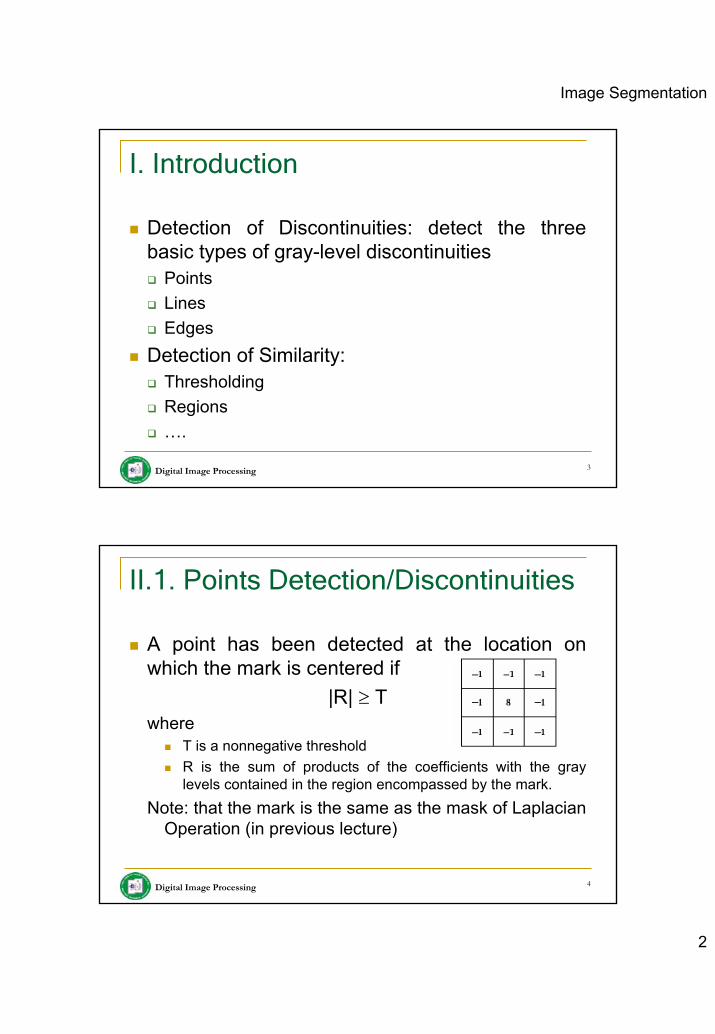
Image Segmentation

2


I. Introduction

Detection of Discontinuities: detect the three basic types of gray-level discontinuities

PointsLinesEdges

Detection of Similarity:ThresholdingRegions….


II.1. Points Detection/Discontinuities

A point has been detected at the location on which the mark is centered if

|R| ≥ Twhere

T is a nonnegative threshold R is the sum of products of the coefficients with the gray levels contained in the region encompassed by the mark.

Note: that the mark is the same as the mask of Laplacian Operation (in previous lecture)

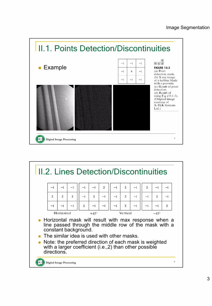
Image Segmentation

3


II.1. Points Detection/Discontinuities

Example


II.2. Lines Detection/Discontinuities

Horizontal mask will result with max response when a line passed through the middle row of the mask with a constant background.The similar idea is used with other masks.Note: the preferred direction of each mask is weighted with a larger coefficient (i.e.,2) than other possible directions.

Image Segmentation

4



Apply every masks on the imageLet R1, R2, R3, R4 denotes the response of the horizontal, +45 degree, vertical and -45 degree masks, respectively.

If, at a certain point in the image |Ri| > |Rj|,

For all j≠i, that point is said to be more likely associated with a line in the direction of mask i.



Apply every masks on the imageLet R1, R2, R3, R4 denotes the response of the horizontal, +45 degree, vertical and -45 degree masks, respectively.

If, at a certain point in the image |Ri| > |Rj|,

For all j≠i, that point is said to be more likely associated with a line in the direction of mask i.

Alternatively, if we are interested in detecting all lines in an image in the direction defined by a given mask, we simply run the mask through the image and threshold the absolute value of the result. The points that are left are the strongest responses, which, for lines one pixel thick, correspond closest to the direction defined by the mask.

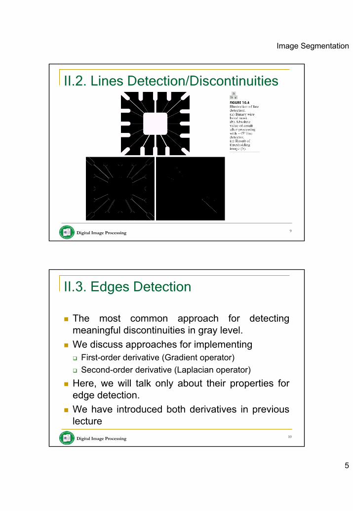
Image Segmentation

5




II.3. Edges Detection

The most common approach for detecting meaningful discontinuities in gray level.We discuss approaches for implementing

First-order derivative (Gradient operator)Second-order derivative (Laplacian operator)

Here, we will talk only about their properties for edge detection.We have introduced both derivatives in previous lecture

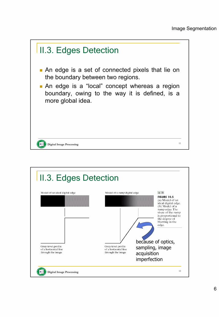
Image Segmentation

6



An edge is a set of connected pixels that lie on the boundary between two regions.An edge is a “local” concept whereas a region boundary, owing to the way it is defined, is a more global idea.



because of optics, sampling, image acquisition imperfection

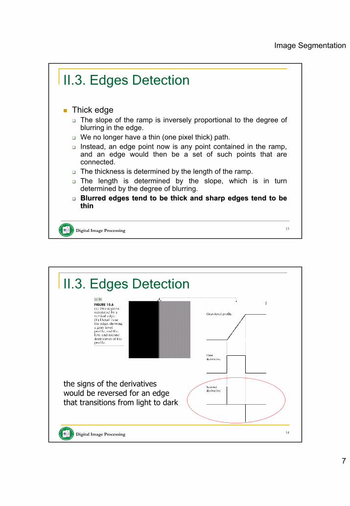
Image Segmentation

7



Thick edgeThe slope of the ramp is inversely proportional to the degree ofblurring in the edge.We no longer have a thin (one pixel thick) path.Instead, an edge point now is any point contained in the ramp, and an edge would then be a set of such points that are connected. The thickness is determined by the length of the ramp.The length is determined by the slope, which is in turn determined by the degree of blurring.Blurred edges tend to be thick and sharp edges tend to be Blurred edges tend to be thick and sharp edges tend to be thinthin



the signs of the derivatives would be reversed for an edge that transitions from light to dark

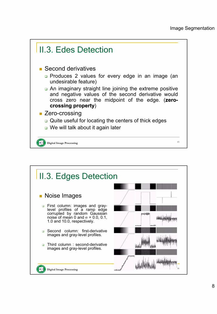
Image Segmentation

8


II.3. Edes Detection

Second derivativesProduces 2 values for every edge in an image (an undesirable feature)An imaginary straight line joining the extreme positive and negative values of the second derivative would cross zero near the midpoint of the edge. (zerozero--crossing propertycrossing property)

Zero-crossingQuite useful for locating the centers of thick edgesWe will talk about it again later



Noise ImagesFirst column: images and gray-level profiles of a ramp edge corrupted by random Gaussian noise of mean 0 and σ = 0.0, 0.1, 1.0 and 10.0, respectively.

Second column: first-derivative images and gray-level profiles.

Third column : second-derivative images and gray-level profiles.

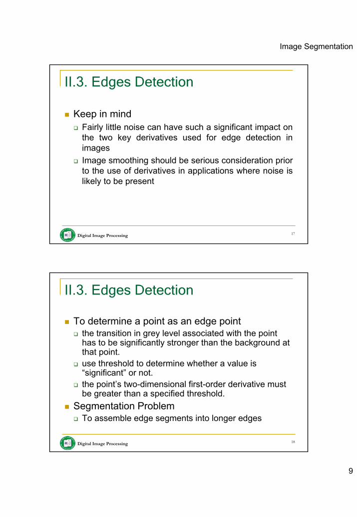
Image Segmentation

9



Keep in mindFairly little noise can have such a significant impact on the two key derivatives used for edge detection in imagesImage smoothing should be serious consideration prior to the use of derivatives in applications where noise is likely to be present



To determine a point as an edge pointthe transition in grey level associated with the point has to be significantly stronger than the background at that point.use threshold to determine whether a value is “significant” or not.the point’s two-dimensional first-order derivative must be greater than a specified threshold.

Segmentation ProblemTo assemble edge segments into longer edges

Image Segmentation

10



Gradient Operators⎥⎥⎥⎥

⎦

⎤

⎢⎢⎢⎢

⎣

⎡

∂∂∂∂

=⎥⎦

⎤⎢⎣

⎡=∇

yfxf

GG

y

xf

21

22

2122 ][)f(

⎥⎥⎦

⎤

⎢⎢⎣

⎡⎟⎟⎠

⎞⎜⎜⎝

⎛∂∂

+⎟⎠⎞

⎜⎝⎛∂∂

=

+=∇=∇

yf

xf

GGmagf yx

yx GGf +≈∇

commonly approx.

First derivatives are implemented using the magnitude magnitude of the gradientof the gradient.



Gradient DirectionLet α (x,y) represent the direction angle of the vector ∇f at (x,y)

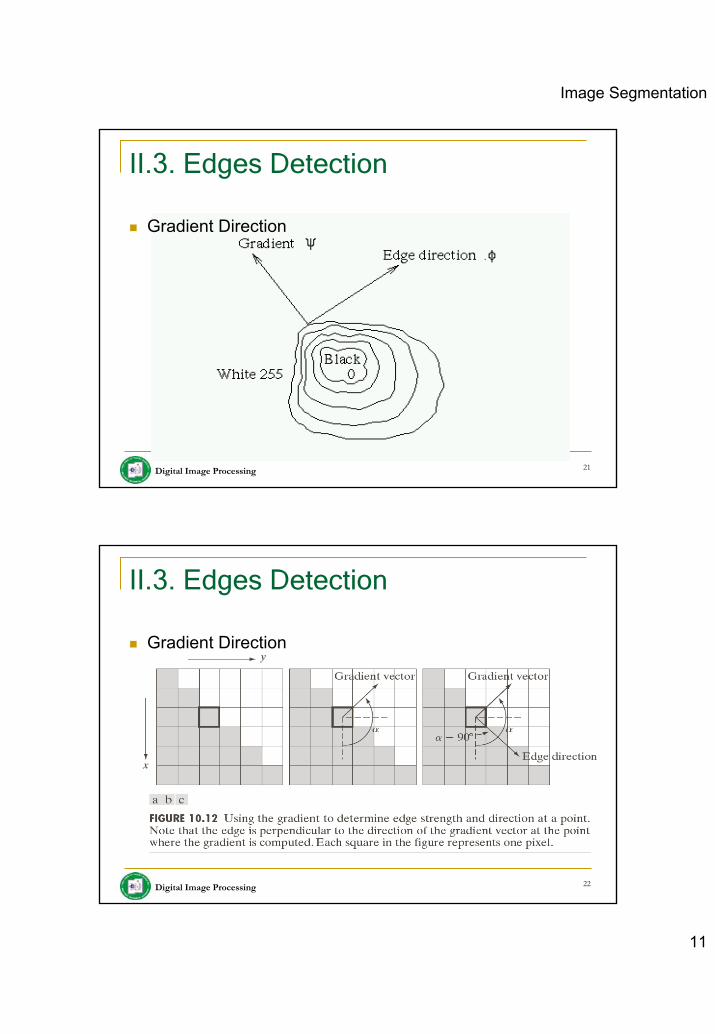
Image Segmentation

11



Gradient Direction



Gradient Direction

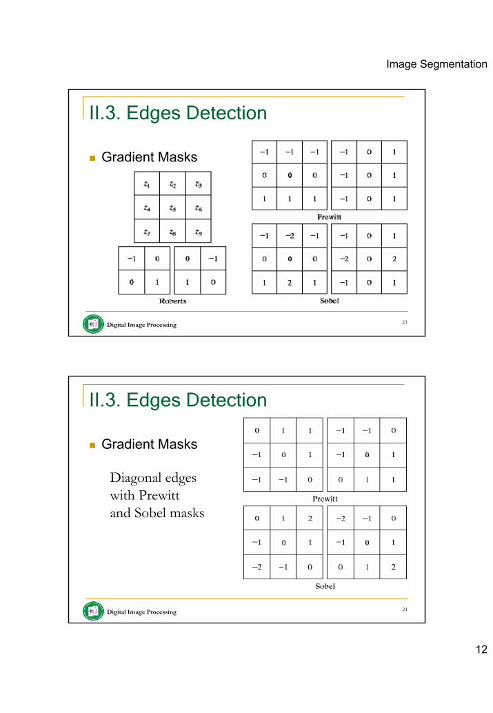
Image Segmentation

12



Gradient Masks



Gradient Masks

Diagonal edges with Prewitt and Sobel masks

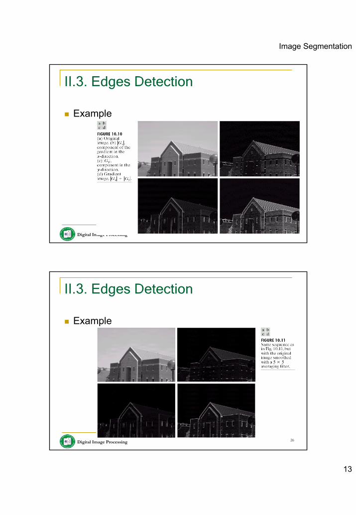
Image Segmentation

13



Example



Example

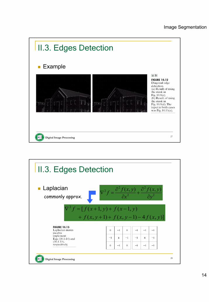
Image Segmentation

14



Example



Laplacian2

2

2

22 ),(),(

yyxf

xyxff

∂∂

+∂

∂=∇

)],(4)1,()1,(),1(),1([2

yxfyxfyxfyxfyxff−−+++

−++=∇

commonly approx.

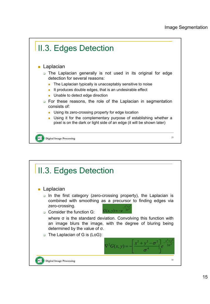
Image Segmentation

15



LaplacianThe Laplacian generally is not used in its original for edge detection for several reasons:

The Laplacian typically is unacceptably sensitive to noiseIt produces double edges, that is an undesirable effectUnable to detect edge direction

For these reasons, the role of the Laplacian in segmentation consists of:

Using its zero-crossing property for edge locationUsing it for the complementary purpose of establishing whether apixel is on the dark or light side of an edge (it will be shown later)



LaplacianIn the first category (zero-crossing property), the Laplacian is combined with smoothing as a precursor to finding edges via zero-crossing.Consider the function G:where σ is the standard deviation. Convolving this function with an image blurs the image, with the degree of bluring being determined by the value of σ.The Laplacian of G is (LoG):

2

22

2),( σyx

eyxG+

−−=

2

22

24

2222 ),( σ

σσ yx

eyxyxG+

−

⎥⎦

⎤⎢⎣

⎡ −+−=∇

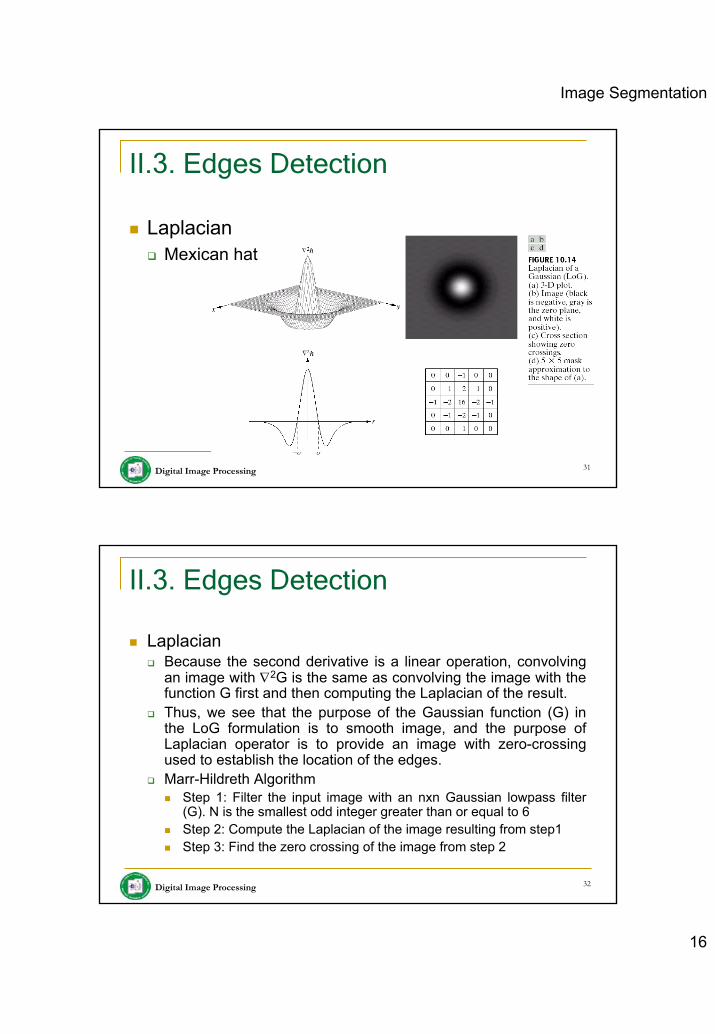
Image Segmentation

16



LaplacianMexican hat



LaplacianBecause the second derivative is a linear operation, convolving an image with ∇2G is the same as convolving the image with the function G first and then computing the Laplacian of the result.Thus, we see that the purpose of the Gaussian function (G) in the LoG formulation is to smooth image, and the purpose of Laplacian operator is to provide an image with zero-crossing used to establish the location of the edges.Marr-Hildreth Algorithm

Step 1: Filter the input image with an nxn Gaussian lowpass filter (G). N is the smallest odd integer greater than or equal to 6Step 2: Compute the Laplacian of the image resulting from step1Step 3: Find the zero crossing of the image from step 2

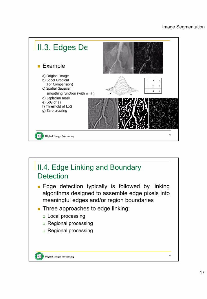
Image Segmentation

17



Examplea) Original imageb) Sobel Gradient

(For Comparision)c) Spatial Gaussian

smoothing function (with σ=5 )d) Laplacian maske) LoG of a)f) Threshold of LoGg) Zero crossing


II.4. Edge Linking and Boundary Detection

Edge detection typically is followed by linking algorithms designed to assemble edge pixels into meaningful edges and/or region boundariesThree approaches to edge linking:

Local processingRegional processingRegional processing

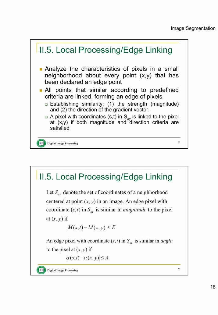
Image Segmentation

18


II.5. Local Processing/Edge Linking

Analyze the characteristics of pixels in a small neighborhood about every point (x,y) that has been declared an edge pointAll points that similar according to predefined criteria are linked, forming an edge of pixels

Establishing similarity: (1) the strength (magnitude) and (2) the direction of the gradient vector.A pixel with coordinates (s,t) in Sxy is linked to the pixel at (x,y) if both magnitude and direction criteria are satisfied



Let denote the set of coordinates of a neighborhood

centered at point ( , ) in an image. An edge pixel with coordinate ( , ) in is similar in to the pixel

at ( , ) if ( ,

xy

xy

S

x ys t S magnitude

x yM s ) ( , )

t M x y E− ≤

An edge pixel with coordinate ( , ) in is similar in

to the pixel at ( , ) if ( , ) ( , )

xys t S angle

x ys t x y Aα α− ≤

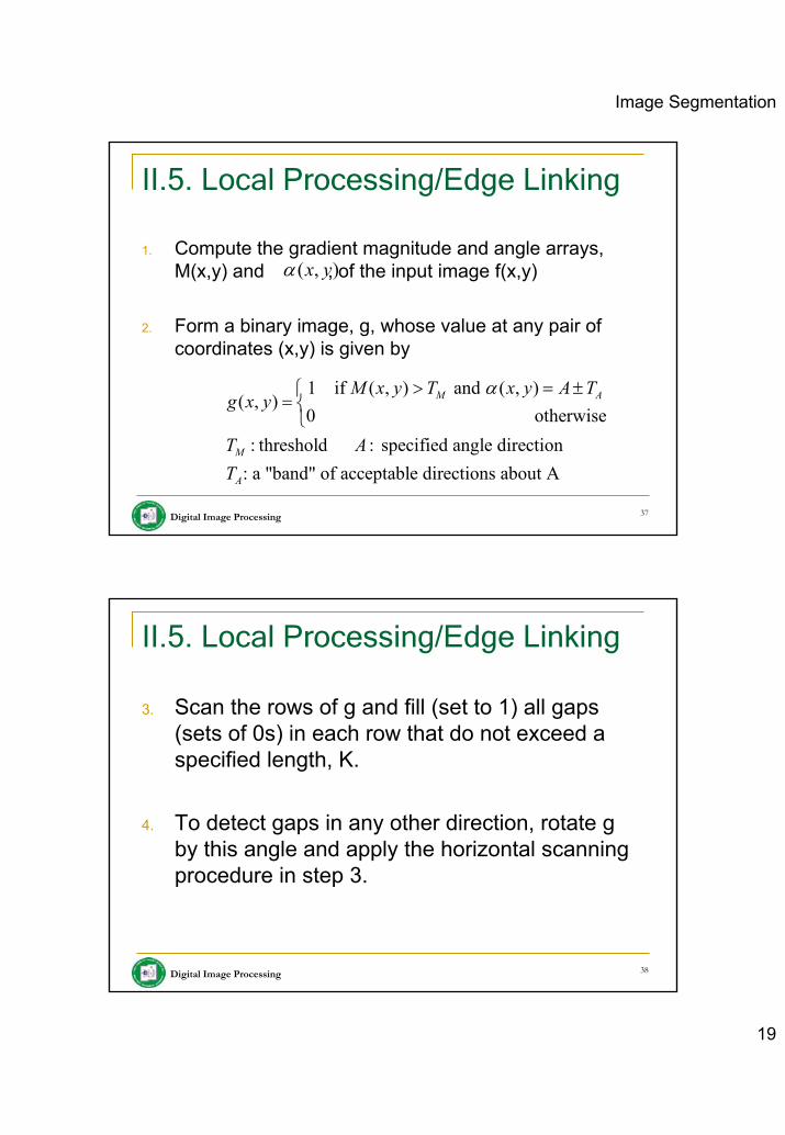
Image Segmentation

19



1. Compute the gradient magnitude and angle arrays, M(x,y) and , of the input image f(x,y)

2. Form a binary image, g, whose value at any pair of coordinates (x,y) is given by

( , )x yα

1 if ( , ) and ( , )( , )

0 otherwise: threshold : specified angle direction

: a "band" of acceptable directions about A

M A

M

A

M x y T x y A Tg x y

T AT

α> = ±⎧= ⎨⎩



3. Scan the rows of g and fill (set to 1) all gaps (sets of 0s) in each row that do not exceed a specified length, K.

4. To detect gaps in any other direction, rotate g by this angle and apply the horizontal scanning procedure in step 3.

Image Segmentation

20



► Example


II.6. Regional Processing/Edge Linking

The location of regions of interest in an image are known or can be determinedPolygonal approximations can capture the essential shape features of a region while keeping the representation of the boundary relatively simpleOpen or closed curveOpen curve: a large distance between two consecutive points in the ordered sequence relative to the distance between other points

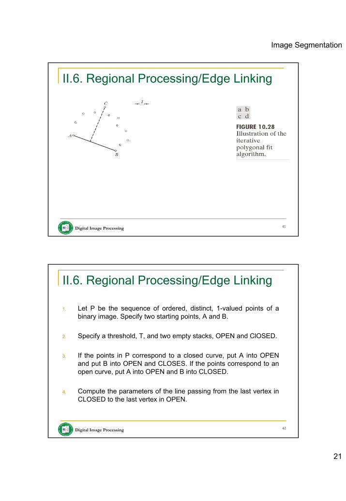
Image Segmentation

21





1. Let P be the sequence of ordered, distinct, 1-valued points of a binary image. Specify two starting points, A and B.

2. Specify a threshold, T, and two empty stacks, OPEN and ClOSED.

3. If the points in P correspond to a closed curve, put A into OPENand put B into OPEN and CLOSES. If the points correspond to an open curve, put A into OPEN and B into CLOSED.

4. Compute the parameters of the line passing from the last vertex in CLOSED to the last vertex in OPEN.

Image Segmentation

22


II.6. Regional Processing/Edge Linking5. Compute the distances from the line in Step 4 to all the points in P

whose sequence places them between the vertices from Step 4. Select the point, Vmax, with the maximum distance, Dmax

6. If Dmax> T, place Vmax at the end of the OPEN stack as a new vertex. Go to step 4.

7. Else, remove the last vertex from OPEN and insert it as the lastvertex of CLOSED.

8. If OPEN is not empty, go to step 4.

9. Else, exit. The vertices in CLOSED are the vertices of the polygonal fit to the points in P.


7. Regional Processing/Edge Linking

Image Segmentation

23



Example



Example

Image Segmentation

24


II.7. Hough Transform/Edge Linking

Example

yi =axi + b b = - axi + yi

ab-plane or parameter spacexy-plane

all points (xi ,yi) contained on the same line must have lines in parameter space that intersect at (a’,b’)


II.7. Hough Transform/Edge Linking

Accumulator cells(amax, amin) and (bmax, bmin) are the expected ranges of slope and intercept values.all are initialized to zeroif a choice of ap results in solution bq then we let A(p,q) = A(p,q)+1at the end of the procedure, value Q in A(i,j) corresponds to Q points in the xy-plane lying on the line y = aix+bj

b = - axi + yi

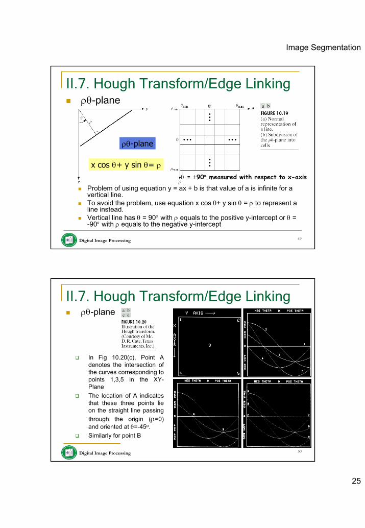
Image Segmentation

25


x cos θ+ y sin θ= ρ

ρθ-plane

II.7. Hough Transform/Edge Linkingρθ-plane

Problem of using equation y = ax + b is that value of a is infinite for a vertical line.To avoid the problem, use equation x cos θ+ y sin θ = ρ to represent a line instead.Vertical line has θ = 90° with ρ equals to the positive y-intercept or θ = -90° with ρ equals to the negative y-intercept

θ = ±90° measured with respect to x-axis


II.7. Hough Transform/Edge Linkingρθ-plane

In Fig 10.20(c), Point A denotes the intersection of the curves corresponding to points 1,3,5 in the XY-PlaneThe location of A indicates that these three points lie on the straight line passing through the origin (ρ=0) and oriented at θ=-45o.Similarly for point B

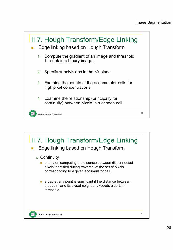
Image Segmentation

26


II.7. Hough Transform/Edge LinkingEdge linking based on Hough Transform

1. Compute the gradient of an image and threshold it to obtain a binary image.

2. Specify subdivisions in the ρθ-plane.

3. Examine the counts of the accumulator cells for high pixel concentrations.

4. Examine the relationship (principally for continuity) between pixels in a chosen cell.



Continuitybased on computing the distance between disconnected pixels identified during traversal of the set of pixels corresponding to a given accumulator cell.

a gap at any point is significant if the distance between that point and its closet neighbor exceeds a certain threshold.

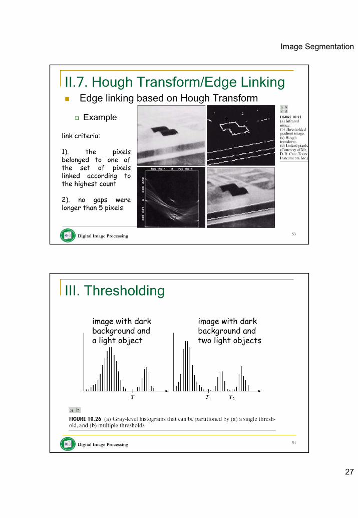
Image Segmentation

27



Example

link criteria:

1). the pixels belonged to one of the set of pixels linked according to the highest count

2). no gaps were longer than 5 pixels


III. Thresholding

image with dark background and a light object

image with dark background and two light objects

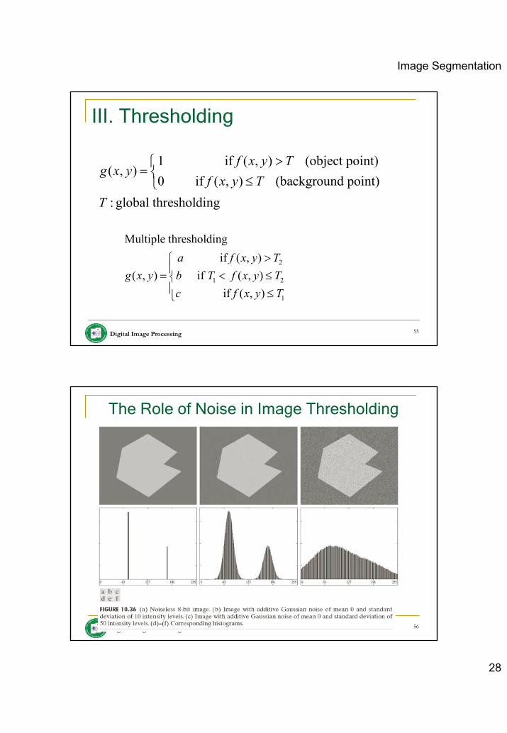
Image Segmentation

28


III. Thresholding

1 if ( , ) (object point)( , )

0 if ( , ) (background point): global thresholding

f x y Tg x y

f x y TT

>⎧= ⎨ ≤⎩

2

1 2

1

Multiple thresholding if ( , )

( , ) if ( , ) if ( , )

a f x y Tg x y b T f x y T

c f x y T

>⎧⎪= < ≤⎨⎪ ≤⎩


The Role of Noise in Image Thresholding

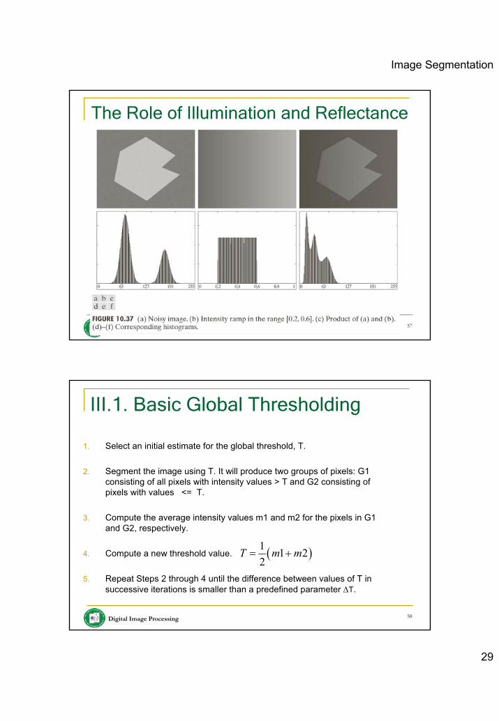
Image Segmentation

29


The Role of Illumination and Reflectance


1. Select an initial estimate for the global threshold, T.

2. Segment the image using T. It will produce two groups of pixels: G1 consisting of all pixels with intensity values > T and G2 consisting of pixels with values <= T.

3. Compute the average intensity values m1 and m2 for the pixels in G1 and G2, respectively.

4. Compute a new threshold value.

5. Repeat Steps 2 through 4 until the difference between values of T in successive iterations is smaller than a predefined parameter ∆T.

III.1. Basic Global Thresholding

( )1 1 22

T m m= +

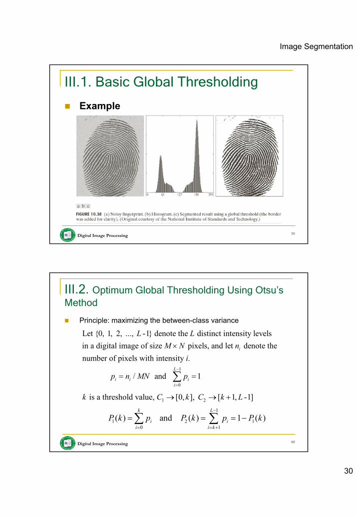
Image Segmentation

30


III.1. Basic Global Thresholding

Example


III.2. Optimum Global Thresholding Using Otsu’s Method

Principle: maximizing the between-class variance

1

0

Let {0, 1, 2, ..., -1} denote the distinct intensity levelsin a digital image of size pixels, and let denote thenumber of pixels with intensity .

/ and 1

i

L

i i ii

L LM N n

i

p n MN p−

=

×

= =∑

1 2 is a threshold value, [0, ], [ 1, -1]k C k C k L→ → +1

1 2 10 1

( ) and ( ) 1 ( )k L

i ii i k

P k p P k p P k−

= = +

= = = −∑ ∑

Image Segmentation

31



1

1 10 01

The mean intensity value of the pixels assigned to classC is

1 ( ) ( / )( )

k k

ii i

m k iP i C ipP k= =

= =∑ ∑

21 1

2 21 12

The mean intensity value of the pixels assigned to classC is

1 ( ) ( / )( )

L L

ii k i k

m k iP i C ipP k

− −

= + = +

= =∑ ∑

1 1 2 2 (Global mean value)GPm P m m+ =



2 2 2

0 1

The optimum threshold is the value, k*, that maximizes ( *), ( *) max ( )B B Bk Lk k kσ σ σ

≤ ≤ −=

1 if ( , ) * ( , )

0 if ( , ) * f x y k

g x yf x y k

>⎧= ⎨ ≤⎩

2

2Separability measure B

G

σησ

=

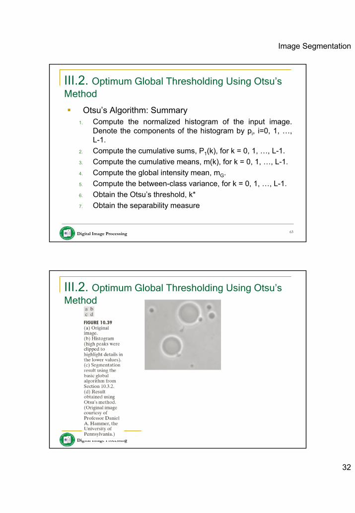
Image Segmentation

32



Otsu’s Algorithm: Summary1. Compute the normalized histogram of the input image.

Denote the components of the histogram by pi, i=0, 1, …, L-1.

2. Compute the cumulative sums, P1(k), for k = 0, 1, …, L-1.3. Compute the cumulative means, m(k), for k = 0, 1, …, L-1.4. Compute the global intensity mean, mG.5. Compute the between-class variance, for k = 0, 1, …, L-1.6. Obtain the Otsu’s threshold, k*7. Obtain the separability measure



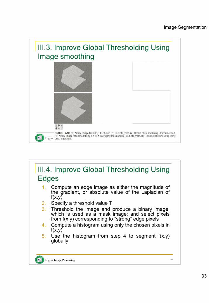
Image Segmentation

33


III.3. Improve Global Thresholding Using Image smoothing


III.4. Improve Global Thresholding Using Edges

1. Compute an edge image as either the magnitude of the gradient, or absolute value of the Laplacian of f(x,y)

2. Specify a threshold value T3. Threshold the image and produce a binary image,

which is used as a mask image; and select pixels from f(x,y) corresponding to “strong” edge pixels

4. Compute a histogram using only the chosen pixels in f(x,y)

5. Use the histogram from step 4 to segment f(x,y) globally

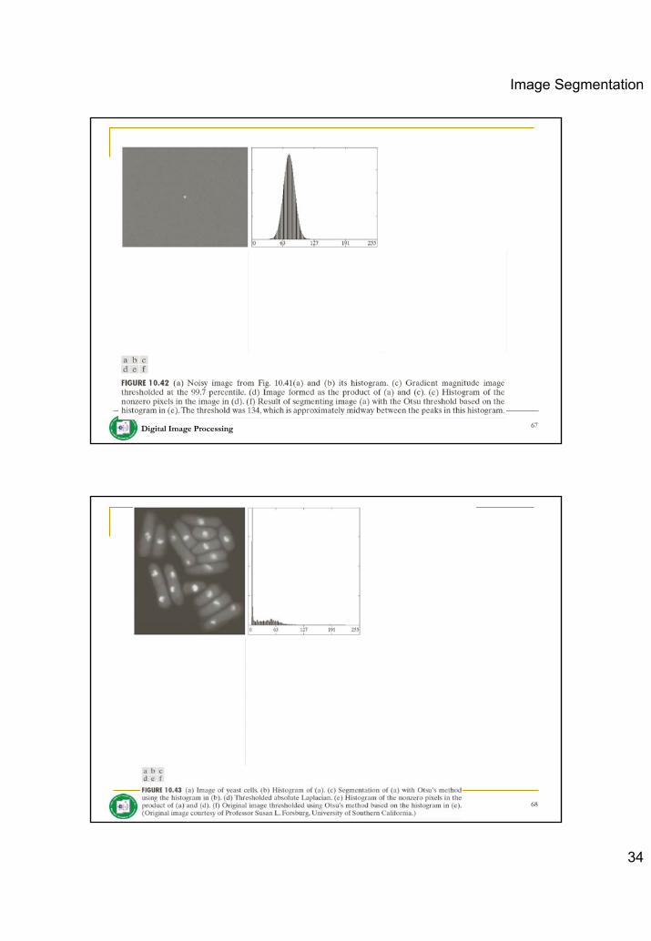
Image Segmentation

34



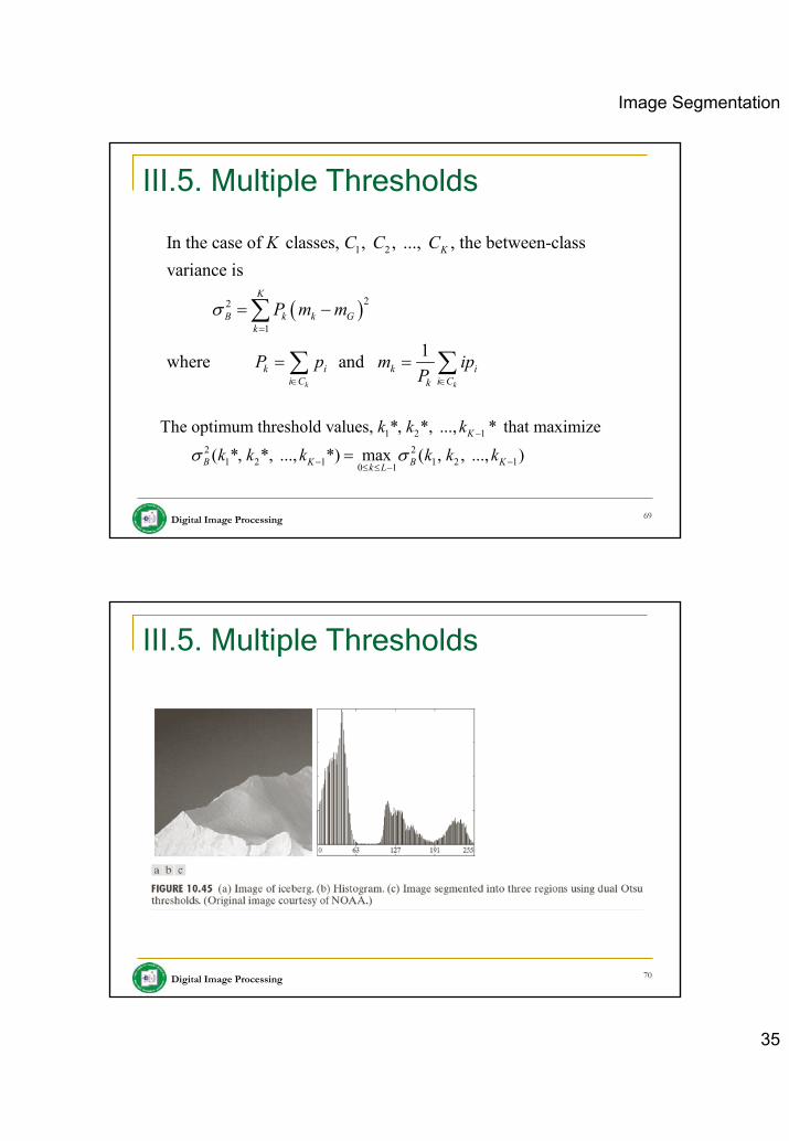
Image Segmentation

35


III.5. Multiple Thresholds

( )

1 2

22

1

In the case of classes, , , ..., , the between-classvariance is

1where and k k

K

K

B k k Gk

k i k ii C i Ck

K C C C

P m m

P p m ipP

σ=

∈ ∈

= −

= =

∑

∑ ∑

1 2 12 2

1 2 1 1 2 10 1

The optimum threshold values, *, *, ..., * that maximize

( *, *, ..., *) max ( , , ..., )K

B K B Kk L

k k k

k k k k k kσ σ−

− −≤ ≤ −=


III.5. Multiple Thresholds

Image Segmentation

36


III.6. Variable Thresholding: Image Partitioning

1. Subdivide an image into nonoverlapping rectangles

2. The rectangles are chosen small enough so that the illumination of each is approximately uniform


14. Variable Thresholding: Image Partitioning

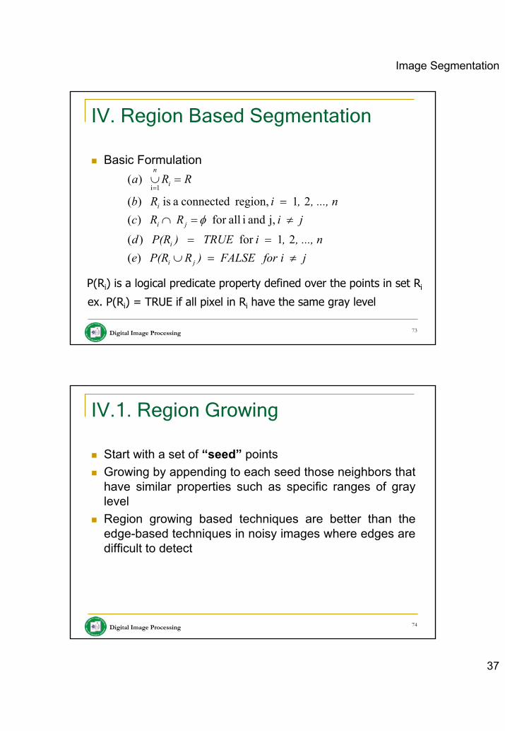
Image Segmentation

37


IV. Region Based Segmentation

Basic Formulation

jfor i FALSE) RP(Re, ..., n, i TRUE) P(Rd

ji RRc, ..., n, i Rb

RRa

ji

i

ji

i

i

n

≠=∪==

≠=∩=

=∪=

)(21for )(

j, and i allfor )(21 region, connected a is )(

)(1i

φ

P(Ri) is a logical predicate property defined over the points in set Ri

ex. P(Ri) = TRUE if all pixel in Ri have the same gray level


IV.1. Region Growing

Start with a set of “seed” pointsGrowing by appending to each seed those neighbors that have similar properties such as specific ranges of gray levelRegion growing based techniques are better than the edge-based techniques in noisy images where edges are difficult to detect

Image Segmentation

38





4-connectivity

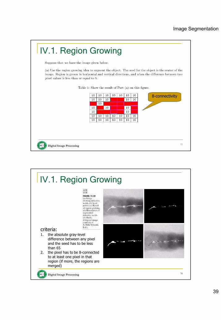
Image Segmentation

39



8-connectivity



criteria:1. the absolute gray-level

difference between any pixel and the seed has to be less than 65

2. the pixel has to be 8-connected to at least one pixel in that region (if more, the regions are merged)

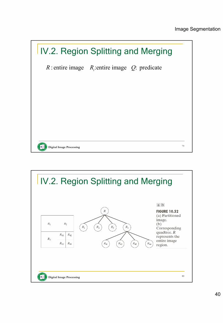
Image Segmentation

40


IV.2. Region Splitting and Merging

: entire image :entire image : predicate

1. For any region , If ( ) = FALSE, we divide the image into quadrants.2. When no further splitting is possible, merge any adjacent regi

i

i i

i

R R Q

R Q RR

ons and

for which ( ) = TRUE.

3. Stop when no further merging is possible.

j k

j k

R R

Q R R∪



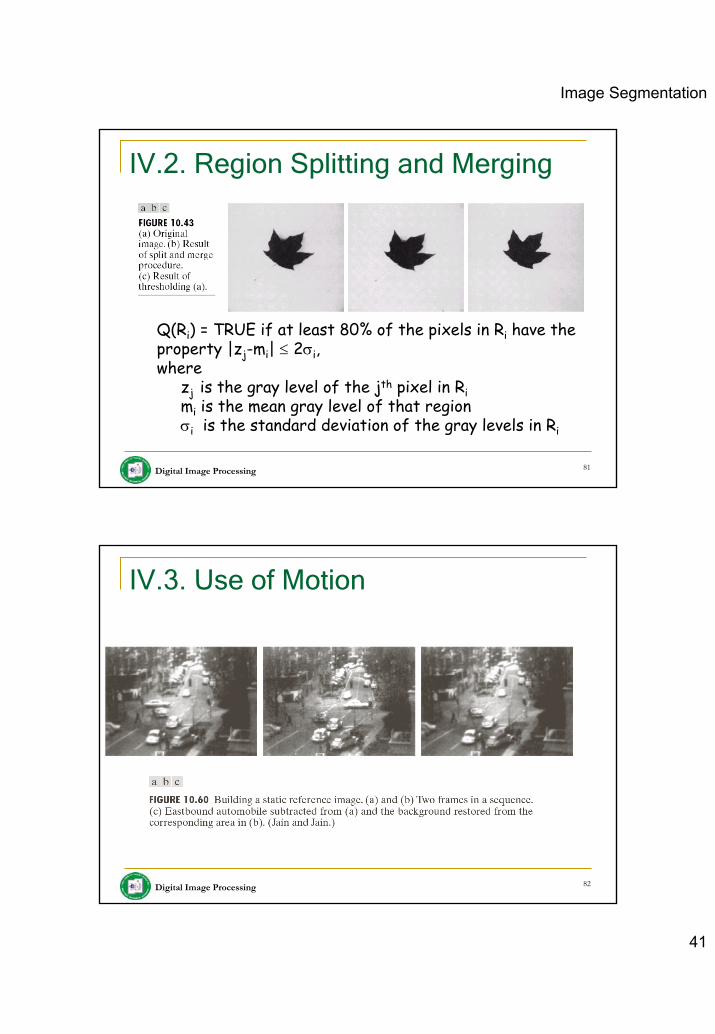
Image Segmentation

41



Q(Ri) = TRUE if at least 80% of the pixels in Ri have the property |zj-mi| ≤ 2σi, where

zj is the gray level of the jth pixel in Rimi is the mean gray level of that regionσi is the standard deviation of the gray levels in Ri


IV.3. Use of Motion

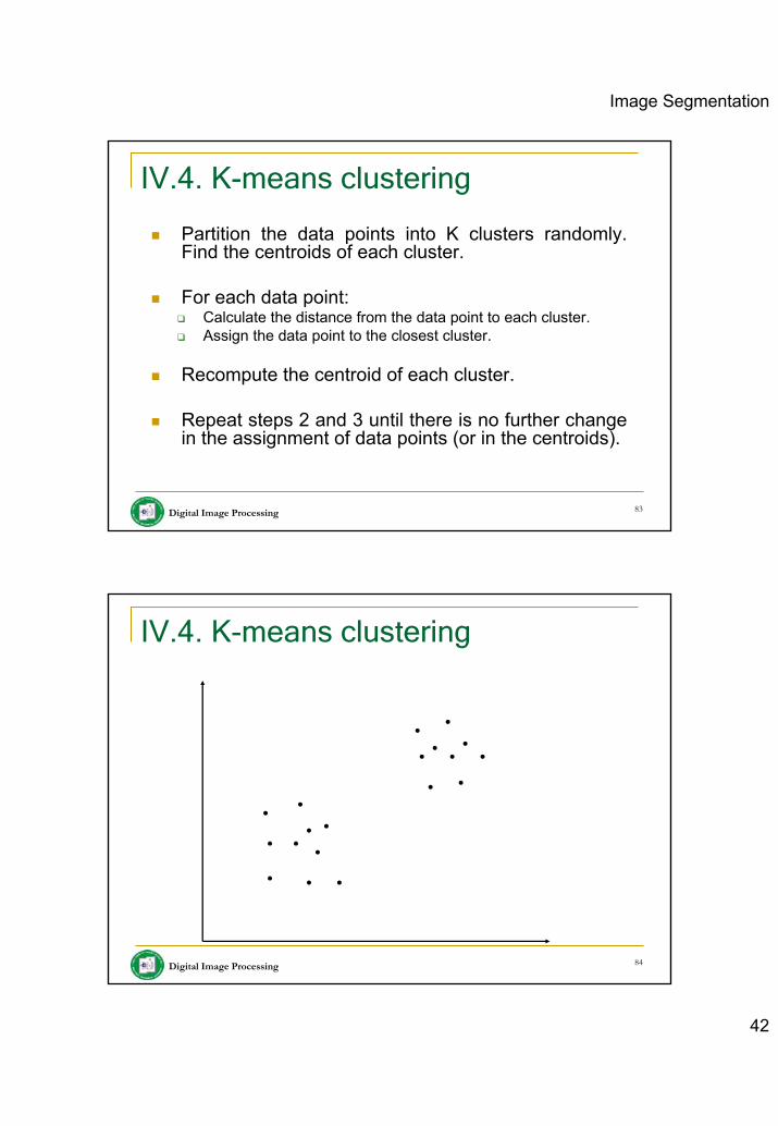
Image Segmentation

42


IV.4. K-means clustering

Partition the data points into K clusters randomly. Find the centroids of each cluster.

For each data point: Calculate the distance from the data point to each cluster.Assign the data point to the closest cluster.

Recompute the centroid of each cluster.

Repeat steps 2 and 3 until there is no further change in the assignment of data points (or in the centroids).



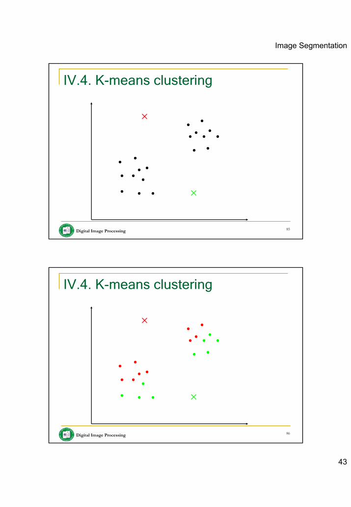
Image Segmentation

43





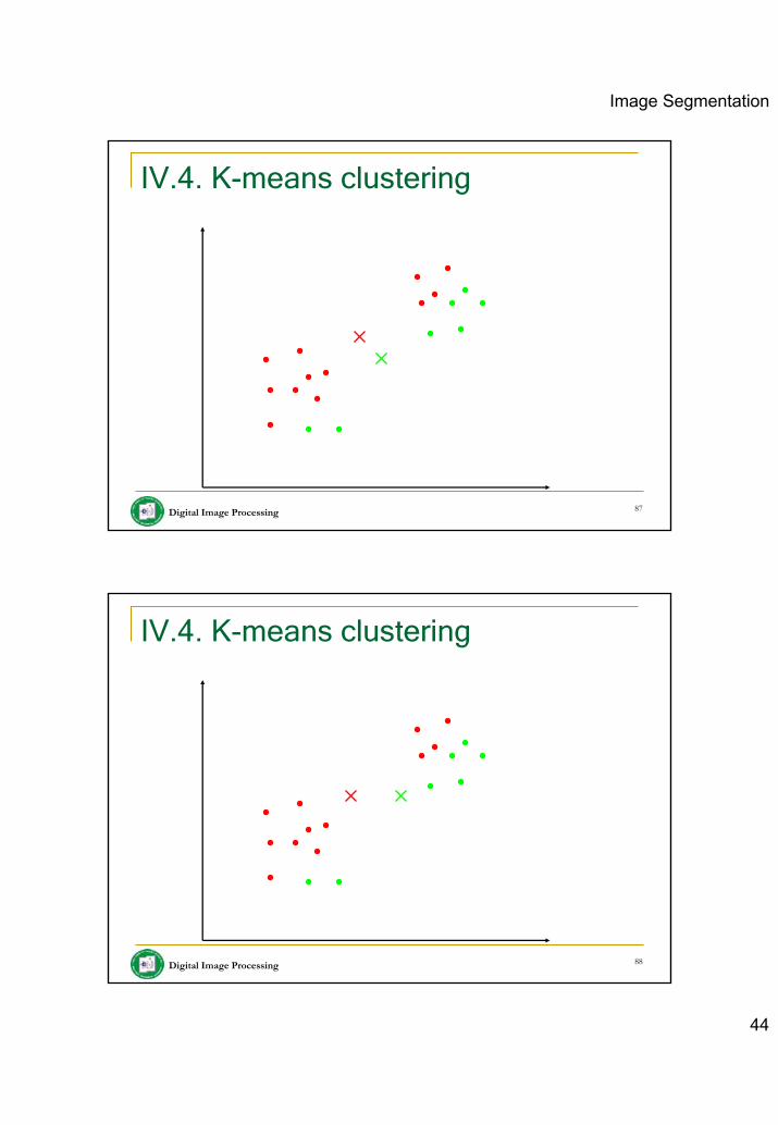
Image Segmentation

44





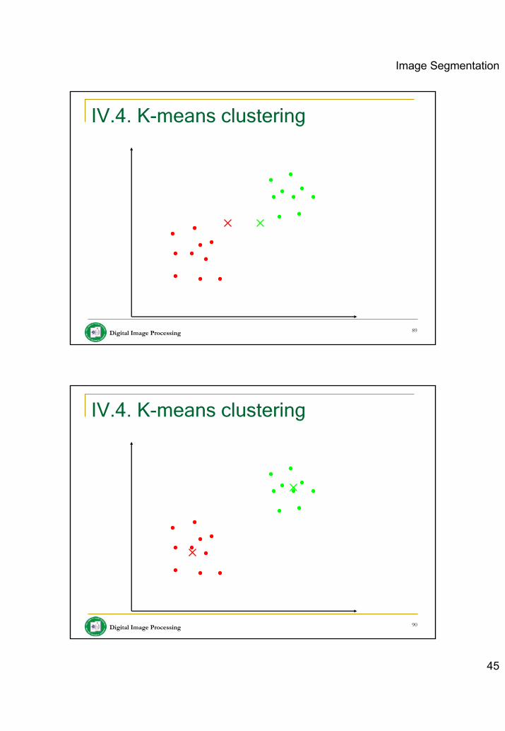
Image Segmentation

45





Documents

Digital Image Processing Lecture 6,7,8 – Image …fit.mta.edu.vn/files/FileMonHoc/Lecture 06,07,08...2006/07/08 · Image Segmentation 1 Digital Image Processing Lecture 6,7,8 –